The GlueX Collaboration
Measurement of the J/ photoproduction cross section over the full near-threshold kinematic region
Abstract
We report the total and differential cross sections for photoproduction with the large acceptance GlueX spectrometer for photon beam energies from the threshold at 8.2 GeV up to 11.44 GeV and over the full kinematic range of momentum transfer squared, . Such coverage facilitates the extrapolation of the differential cross sections to the forward () point beyond the physical region. The forward cross section is used by many theoretical models and plays an important role in understanding photoproduction and its relation to the proton interaction. These measurements of photoproduction near threshold are also crucial inputs to theoretical models that are used to study important aspects of the gluon structure of the proton, such as the gluon Generalized Parton Distribution (GPD) of the proton, the mass radius of the proton, and the trace anomaly contribution to the proton mass. We observe possible structures in the total cross section energy dependence and find evidence for contributions beyond gluon exchange in the differential cross section close to threshold, both of which are consistent with contributions from open-charm intermediate states.
I Introduction
Over the past several years there has been a renewed interest in studying near-threshold photoproduction as a tool to experimentally probe important properties of the nucleon related to its gluon content. Such experiments became possible thanks to the GeV upgrade of the CEBAF accelerator at Jefferson Lab covering the threshold region of the reaction, resulting in the first exclusive measurements very close to threshold by the GlueX collaboration Ali et al. (2019) (GlueX collaboration).
Exclusive photoproduction is expected to proceed dominantly through gluon exchange due to the heavy mass of the charm quark. Thus, the dependence of the reaction is defined by the proton vertex, which provides a probe of the nucleon gluon form factors Frankfurt and Strikman (2002). The extraction of the gluonic properties of the proton from production data requires additional assumptions. One such assumption is the use of Vector Meson Dominance (VMD) to relate the reaction to elastic scattering. At low energies, the latter reaction is related to several fundamental quantities. These include the trace anomaly contribution to the mass of the proton Kharzeev et al. (1999); Hatta and Yang (2018); Kou et al. (2021), and the scattering length which is related to the possible existence of a charmonium-nucleon bound state Strakovsky et al. (2020); Pentchev and Strakovsky (2021).
An important QCD approach is to assume factorization between the gluon Generalized Parton Distributions (gGPD) of the proton and the wave function, and the hard quark-gluon interaction. The hard scale in this approach is defined by the heavy quark mass. In Ref. Ivanov et al. (2004) such a general approach was applied to the photoproduction in leading-order (LO) and next-to-leading-order (NLO) at high energy and small transferred momentum . An important continuation of these efforts can be found in Refs. Hatta and Strikman (2021); Guo et al. (2021), where it was shown in LO and for heavy quark masses, that factorization also holds at energies down to threshold for large absolute values of . Close to threshold, due to the large skewness parameter, the spin-2 (graviton-like) two-gluon exchange dominates Hatta and Strikman (2021) and therefore photoproduction can be used to study the gravitational form factors of the proton Guo et al. (2021). Such information was used to estimate the mass radius of the proton Kharzeev (2021); Ji et al. (2021); Mamo and Zahed (2021a); Wang et al. (2021), as opposed to the well-known charge radius. Alternatively, the holographic approach was used to describe the soft part of photoproduction and relate the differential cross sections to the gravitational form factors Hatta and Yang (2018); Hatta et al. (2019); Mamo and Zahed (2020, 2021a, 2021b).
However, such an ambitious program to study the mass properties of the proton requires detailed investigation of the above assumptions used to interpret the data. Ref. Sun et al. (2022) calculates directly Feynman diagrams of the near threshold heavy quarkonium photoproduction at large momentum transfer and finds that there is no direct connection to the gravitational form factors. In contrast to the above gluon-exchange mechanisms, it was proposed in Ref. Du et al. (2020) that exclusive photoproduction may proceed through open-charm exchange, namely . The authors point out that the thresholds for these intermediate states are very close to the threshold and their exchange can contribute to the reaction. They predict cusps in the total cross section at the and thresholds. If such a mechanism would dominate over the gluon-exchange mechanism, it would obscure the relation between exclusive photoproduction and the gluonic properties of the proton together with all the important physical implications discussed above.

Furthermore, understanding the contribution of any processes besides gluon exchange to photoproduction is crucial for the search for the photoproduction of the LHCb pentaquark candidates Aaij et al. (2015, 2019). The states can be produced in the -channel of the reaction, and the strength of this resonant contribution can be related to the branching fraction of under the assumptions of VMD and a dominant non-resonant gluon exchange Wang et al. (2015); Kubarovsky and Voloshin (2015); Karliner and Rosner (2016); Blin et al. (2016). If there would be significant contributions from other processes such as the open-charm exchange mentioned above, both of these assumptions break down. Therefore, a better understanding of all the processes that contribute to photoproduction is required before updated searches for the can be performed.
In this work we report on the measurement of exclusive photoproduction,
| (1) |
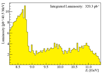
based on the data collected by Phase-I of the GlueX experiment Adhikari et al. (2021) during the period . This data sample is more than four times larger than the one used in the first GlueX publication Ali et al. (2019) (GlueX collaboration). We present results for the total cross section for photon beam energies from threshold, , up to GeV. We also present the differential cross sections, , in three regions of photon beam energy over the full kinematic space in momentum transfer , from to , thanks to the full acceptance of the GlueX detector for this reaction. We identify the particle through its decay into an electron-positron pair. Due to the wide acceptance for the exclusive reaction , we observe events in a broad range of invariant masses, including peaks corresponding to the and mesons and the continuum between the two peaks that is dominated by the non-resonant Bethe-Heitler (BH) process (see Fig. 1). As an electromagnetic process that is calculable to a high accuracy, we will use the measurement of this BH process for the absolute normalization of the photoproduction cross sections.
II The GlueX detector
The experimental setup is described in detail in Ref. Adhikari et al. (2021). The GlueX experiment uses a tagged photon beam, produced on a diamond radiator from coherent Bremsstrahlung of the initial electron beam from the CEBAF accelerator. The scattered electrons are deflected by a Tm dipole magnet and detected in a tagging array which consists of scintillator paddles and fibers, that allows determination of the photon energy with resolution. The photons are collimated by a 5 mm diameter hole placed at m downstream of the radiator. The flux of the photon beam is measured with a pair spectrometer (PS) Barbosa et al. (2015) downstream of the collimator, which detects electron-positron pairs produced in a thin converter. For most of Phase-I, the electron beam energy was GeV, corresponding to about GeV maximum tagged photon energy. The coherent peak was kept in the region of GeV, which is just above the threshold, see Fig. 2. The produced photon beam is substantially linearly polarized in this peak region and the orientation of the polarization was changed periodically, although the beam polarization was not used in this analysis. The bunches ( ps long) in the electron and secondary photon beams are ns apart for almost all of the data.
The GlueX detector is built around a T solenoid, which is 4 m long and has an inner diameter of the bore of m. A liquid Hydrogen target that is cm long, is placed inside the magnet. It is surrounded by a Start Counter Pooser et al. (2019), a segmented scintillating detector with a timing resolution of to ps, that helps us to choose the correct beam bunch. The tracks of the final state charged particles are reconstructed using two drift chamber systems. The Central Drift Chamber (CDC) Jarvis et al. (2020) surrounds the target and consists of 28 layers of straw tubes (about in total) with axial and stereo orientations. The low amount of material in the CDC allows tracking of the recoil protons down to momenta as low as GeV and identify them via the energy losses for GeV. In the forward direction, but still inside the solenoid, the Forward Drift Chamber (FDC) Pentchev et al. (2017) system is used to track charged particles. It consists of 24 planes of drift chambers grouped in four packages with both wire and cathode-strip (on both sides of the wire plane) readouts, in total more than channels. Such geometry allows reconstruction of space points in each plane and separation of trajectories in the case of high particle fluxes present in the forward direction.
Electrons and positrons are identified by two electromagnetic calorimeters. The Barrel Calorimeter (BCAL) Beattie et al. (2018) is inside the magnet and surrounds the two drift chamber systems. It consists of lead layers and scintillating fibers, grouped in 192 azimuthal segments and four radial layers, allowing reconstruction of the longitudinal and transverse shower development. The Forward Calorimeter (FCAL) covers the downstream side of the acceptance outside of the magnet at about m from the target and consists of 2800 lead-glass blocks of () cm3. A Time-of-Flight scintillator wall is placed just upstream of the FCAL.
The two calorimeters, BCAL and FCAL, are used to trigger the detector readout with a requirement of sufficient total energy deposition. The trigger threshold is optimized for the collection of minimum ionizing events and is much lower than the sum of the energy of the two leptons for the reactions discussed in this paper. The intensity of the beam in the energy region above the threshold gradually increased from about photons/s in 2016 to about photons/s at the end of 2018, resulting in a total integrated luminosity of pb-1.
III Data Analysis
A key feature of our measurement is that the GlueX detector has essentially full acceptance for the photoproduction in Eq. 1. For photoproduction of light mesons, the acceptance of the recoil proton is limited at low momentum where the protons do not reach the drift chambers. However, due to the high mass of the meson, the recoil proton has a minimum momentum of GeV and can be reliably detected. Geometrically, the GlueX detector has full azimuthal acceptance and polar angle coverage, allowing detection of all the final state particles in the whole kinematic region of the reaction. Thus, the total cross section of the exclusive reaction is measured directly, without any assumptions about the final state particles or extrapolations to kinematic regions outside of the acceptance.
The three final state particles are required to originate within the time of the same beam bunch. The beam photons whose time (as determined by the tagger) coincide with this bunch are called in-time photons and they qualify as candidates associated with this event. The other, out-of-time, tagged photons are used to estimate the fraction of events that are “accidentally” associated with an in-time photon that did not produce the reconstructed final state particles. Unless otherwise noted, all the distributions shown in this paper have the corresponding accidental background contributions subtracted.
The exclusivity of the measurement, together with the precise knowledge of the beam energy and its direction, allows performing of a kinematic fit. The fit requires four-momentum conservation and a common vertex of the final state particles. A very loose selection criterion is applied to the value of the fit. The momentum of the recoil proton, is relatively well measured, as the protons are produced at moderate polar angles () with GeV. This is not the case for the lepton pair, where one of the leptons is predominantly produced with a high momentum at a small polar angle, i.e. in a region with a poor momentum resolution of the solenoidal spectrometer. The kinematic fit to the full reaction is therefore constrained mainly by the direction and magnitude of the proton momentum and the direction of the lepton momenta, which are measured more precisely than the magnitudes of the lepton momenta. After applying the kinematic fit, the mass resolution improves significantly to about MeV (see Fig. 1).
Monte Carlo simulations for both and BH processes have been performed. To calculate the absolute BH cross section, we have used a generator Paremuzyan (2017) based on analytic calculations of the BH cross sections Berger et al. (2002). For the proton form factors that enter in the calculations, we use the low- parametrization of Ref. Borah et al. (2020). We note that if the dipole form factors are used instead, the BH cross section differs by less than 1% within the kinematic region used for normalization. The events were generated using a -dependence and an energy dependence of the cross section obtained from smooth fits to our measurements. For the decay, photon-to- spin projection conservation in the Gottfried-Jackson frame is assumed. This corresponds to a angular distribution of the decay particles, where is the lepton polar angle in the Gottfried-Jackson frame.
To simulate the detector response we have used the GEANT4 package Allison et al. (2016). In addition, to the generated events, we include accidental tagger signals and detector noise hits extracted from data collected with an asynchronous trigger. These simulations are used to calculate the reconstruction efficiencies for the two processes, and . The BH simulations are also used to integrate the absolute cross sections in the kinematic regions used for normalization.
We use the BH process in the invariant mass region of GeV for the absolute normalization of the total cross section, thus eliminating uncertainties from sources like luminosity and reconstruction efficiencies that are common for both processes. The main challenge in extracting the BH yields is to separate the pure continuum from the background of production that is more than three orders of magnitude more abundant. We suppress the pions primarily using the energy deposition in the calorimeters and requiring both lepton candidates to have consistent with unity, where is the momentum determined from the kinematic fit. In addition, we use the inner layer of the BCAL as a pre-shower detector and require the energy deposition there to be MeV, where corrects for the path length in the pre-shower layer. The pion background is further reduced by selecting the kinematic region with particle momenta GeV, to remove pions coming from target excitations. In addition, for the BH measurements only, we select GeV2 as the BH cross section is dominated by the pion background above this -value, due to the very sharp -dependence of the BH process. After applying all of the selection criteria above, the remaining background is of approximately the same magnitude as the signal. The final BH yields are extracted by subtracting this pion background using the procedure described below.
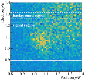
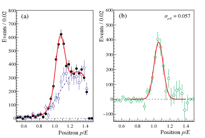
We extract the yields of the leptons detected in the BCAL and FCAL separately, since the calorimeters have different resolutions. We perform this procedure in bins of the beam energy or other kinematic variables. For illustration only, in Figs. 3 and 4 we demonstrate this procedure over one energy bin ( GeV) including leptons detected in both calorimeters. We consider the two-dimensional distribution of electron vs. positron candidates, and define a one-dimensional signal region around the peak of one of the leptons. The projection of this region onto the axis of the second lepton is shown in Fig. 4(a) (full black points). The shape of the pion background is estimated using events outside of the peak of the first lepton (the background region indicated in Fig. 3), to which we fit a polynomial function of third order. The events in the signal region (full black points in Fig. 4(a)) are then fit with a sum of a Gaussian and this polynomial, where the latter is multiplied by a free normalization parameter, . The background distribution scaled by is shown by the open blue points in Fig. 4(a). The lepton yields are extracted by fitting the difference of the distribution in the signal region (full black points) and the scaled background distribution (open blue points) with a Gaussian, shown in Fig. 4(b). We perform this procedure for both positrons and electrons. For each species, the yields are extracted separately for the cases where the selected lepton is detected by the BCAL or the FCAL (regardless of where the other lepton is detected). We then average the summed yields for electrons and positrons to estimate the BH yields. To estimate the systematic uncertainty of this procedure at each data point, two variations of the method are tested. They differ by fixing the width of the peak to the simulations (default for the central value) or leaving it as a free parameter. We also vary the method of integrating the signal, either by summing the histogram values in Fig. 4(b) (default) or integrating the fitted function. The results of these variations are discussed in Sec. 9.
As a check of the validity of our reconstruction procedure, we extract the BH cross section from our data and compare it to the expectations from the absolute calculations described previously. The fitting procedure described above is applied in bins of various kinematic quantities, e.g. , and we extract the cross section as:
| (3) |
where is the measured BH yield in a specific photon-energy bin, is the corresponding reconstruction efficiency determined from MC simulations, and is the measured luminosity. We note that the photon beam luminosity is used just for this study as a cross check, but not for the final cross sections that are determined relative to these BH cross sections.
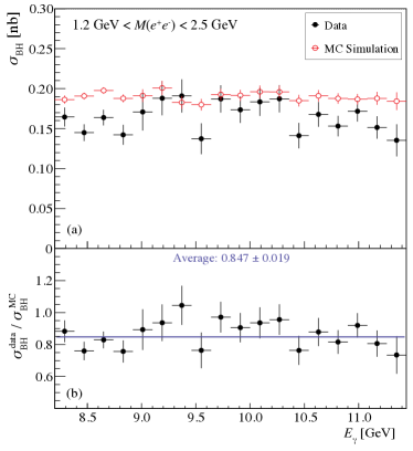
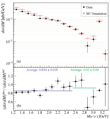
The BH cross sections as function of the beam energy, extracted from Eq. (3), are compared with the MC calculations in Fig. 5. The data/MC ratio of the cross sections (Fig. 5(b)) is consistent with a constant and differs from unity by about . Since this ratio is approximately constant over the kinematic region under consideration, we take its difference from unity as an estimation of the overall systematic uncertainty in the normalization of our cross sections. Similar ratios as a function of other kinematic variables, including proton momentum and polar angle, have been studied. Although the BH cross section varies by up to two orders of magnitude across these variables, the data and MC results remain consistent. In Fig. 6 we show one such comparison as a function of the invariant mass, , which illustrates how well the BH simulations describe the data from the region used for normalization ( GeV) to the peak. We see a slight increase in the data/MC ratio in the region close to the peak, which, however, is not statistically significant and is within the uncertainty estimated above.
To measure the yields, we apply the same event selections as for the BH process described above, except that we do not constrain the range. We select lepton candidates using selections, however, in contrast to the BH continuum, no additional fitting procedure is needed to separate the pion background. Instead, we separate candidates from the background by fitting the narrow peak in the distributions. We fit the mass distributions in 18 bins of the beam energy with a Gaussian for the peak plus a linear background. Because of the fine binning and the resulting small sample size in each bin, we employ the binned maximum-likelihood method, where Poisson errors are assumed in each invariant-mass bin, using the RooFit package Verkerke and Kirkby . Our studies show that the background due to accidental beam photon combinations in this mass region is small (about ) and of similar shape to the other smooth backgrounds, so in this case we do not explicitly subtract these accidental combinations. We perform fits, where we leave the Gaussian width of the peak as a free parameter and where we fix it to the expectation from MC simulation. The fitted widths of the peaks match well the expectations from simulation. We hence fix the widths to obtain our nominal results and use the results with free widths to estimate the systematic uncertainty in our knowledge of the peak shape. To study the systematic uncertainty of the lepton identification we also vary the selections, and include these variations as described below.
IV Total cross section
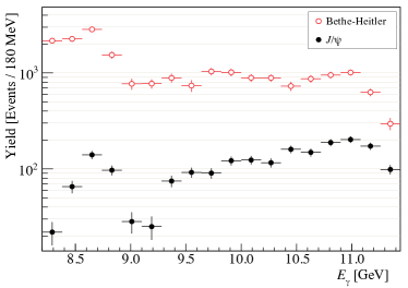
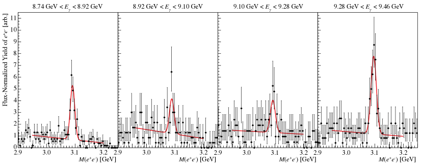
The extracted and BH yields as a function of beam energy are compared in Fig. 7. While the BH yields follow the beam intensity spectrum, the yields exhibit an indication of a dip in the GeV region which will be discussed below. For illustration, individual mass fits for four energy bins around GeV are shown in Fig. 8. The beam photon flux varies strongly in this region, so to correct for this effect we scale the yield by the flux for the corresponding energy bin.
We calculate the total cross section as a function of beam energy using the following formula:
| (5) |
Here and are the corresponding yields, is the calculated BH cross section integrated over the region used for normalization, is the branching ratio of Tanabashi et al. (2018) (Particle Data Group), and and are the MC-determined efficiencies. Note that only the relative efficiency between the two processes enters in the above equation.
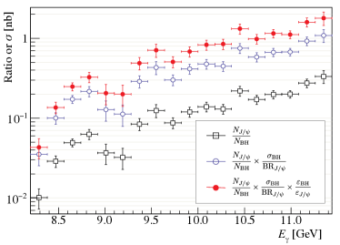
The calculations in Eq.(5) are shown in several steps in Fig. 9 to demonstrate that the possible dip structure at GeV arises from the yield ratio and not from the subsequent corrections. We note that the position of the dip coincides with a drop in the photon-beam intensity just above the coherent peak, as seen in Fig. 2, however we perfomed studies showing that this is coincidental. In particular, as seen in Fig. 7, there is no dip in the BH yields in this region. Since the reconstruction of the final state is strongly determined by the reconstruction of the recoil proton, we have also searched for a similar deviation in photoproduction, , where we require the invariant mass to be in the mass region GeV. With this selection, the recoil protons in this reaction are kinematically close to those in the reaction. We find that the flux normalized yields for the reaction as a function of photon energy are smooth in the region of the dip.
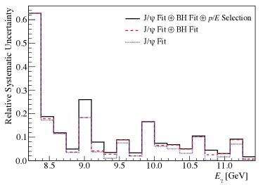
The systematic uncertainties on the individual cross section points are taken from three sources as previously described. The systematic uncertainty in the BH yield extraction is determined by the maximum deviation in the two fitting variations from the nominal value, as discussed above. The systematic uncertainty in the yield extraction is determined by taking the difference in the cross section values between the fits with fixed and free Gaussian widths. Additionally, we study the deviation in the cross section when widening the selected region around the peak to . To estimate this uncertainty, we use the photon flux instead of the BH cross section to calculate the cross section. This change in the normalization is required due to the difficulty of measuring the BH cross section with this looser requirement. The uncertainties from each of the three contributions are added in quadrature to get the total systematic uncertainties. These values are illustrated in Fig. 10.
As mentioned above, we assume in the MC simulation a certain angular distribution of the decay products, namely , where is the lepton polar angle in the Gottfried-Jackson frame, which corresponds to photon-to- conservation of the spin projection in this frame. To estimate the systematic error related to this assumption, we compare the efficiency from this model to the extreme case when assuming uniform distribution. The variations of the efficiency as a function of energy do not exceed . We also perform a fit to the measured distribution and find the results to be consistent with the assumption of spin projection conservation, which reduces the above upper limit on this uncertainty to a level.
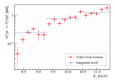
The measured total cross section is plotted in Fig. 11, with the statistical and total uncertainties shown separately. With the exception of the first point, the statistical errors dominate. The numerical results for the total cross section, along with their statistical and systematic errors, are given in Table 3 of the Appendix, Sec. A.
The summary of the sources and magnitudes of the overall normalization uncertainties is given in Table 1. The main source of this uncertainty was discussed in Section III, where we studied the BH data/MC ratio as a function of the beam energy and invariant mass. We use the average difference between data and MC, that is consistent with a constant function of energy (see Fig.5), as a measure of the systematic uncertainty in the overall scale. The effect of the radiative corrections to the cross section was studied in the previous publication Ali et al. (2019) (GlueX collaboration) based on Ref. Heller et al. (2018). The possible contribution of the Time-like Compton Scattering (TCS) to the continuum was estimated in Ali et al. (2019) (GlueX collaboration) using a generator Boer (2019) based on the calculations in Ref.Boer et al. (2015). To estimate the effect of a possible contribution of to the region used for normalization, we fit the data/MC ratio vs. invariant mass in Fig. 6 with constants in two regions, the standard one GeV and the one over the resonance region GeV. The results are and , respectively. These results are consistent within the combined error, which we conservatively take as a measure of this systematic uncertainty.
| Source | Uncertainty |
|---|---|
| BH data-to-MC ratio vs. | |
| Radiative corrections | |
| TCS contribution to BH | |
| contribution to BH | |
| Total |
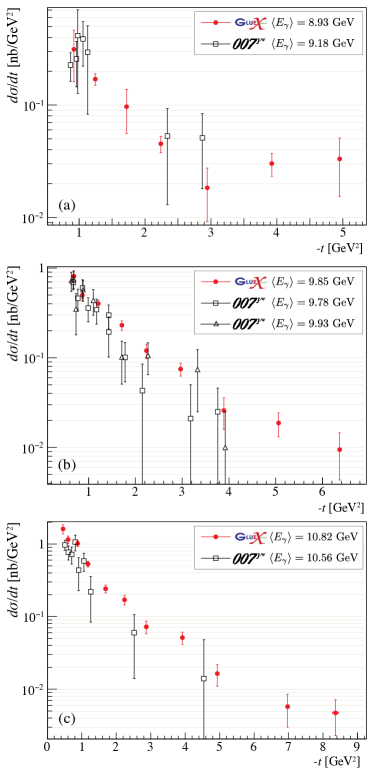
V Differential cross sections
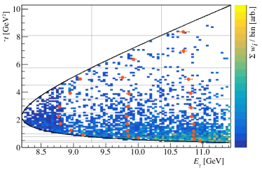
We present measurements of the differential cross sections, , over the entire near-threshold kinematic region. The two-dimensional bins in the () plane for which we report the cross section values are shown in Fig. 12. We subdivide the data into three equidistant energy ranges, while the -bins match the crossing of these ranges with the and kinematic limits. Such a choice allows sufficient sample size in each bin. Because the variation of the beam-photon flux across each energy bin is rather large, we weight each event by the measured luminosity in steps of MeV bins, i.e. the weight for bin is:
| (7) |
We then fit the weighted distribution to obtain a luminosity-weighted number of events in each bin of and , which we denote . The energy resolution as measured by the experimental setup is better than the MeV bin size used in this procedure.
The cross sections are reported at the mean and values within each bin (red points in Fig. 12). Note that for a given energy region, the mean values depend on the bin. Still, we attribute a common mean energy within each energy region and treat the corresponding deviations of the cross section due to the energy correction as a systematic error. In addition, generally, the cross section averaged over the bin deviates from the cross section at the mean and where it is reported, especially for the bins that are wide and have non-rectangular shapes. This deviation will also be treated as a systematic error.
To calculate the differential cross section, we divide the luminosity-weighted number of events in each bin by the area of the bin, , and correct for the reconstruction efficiency :
| (9) |
Thus, the differential cross section will be in units of [nb/GeV2]. The area of each bin is calculated with MC by generating a uniform distribution over the whole rectangular () plane in Fig. 12.
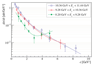
We apply the same procedure for the extraction of the yields as explained in Sec. 6 for the total cross section. The efficiencies calculated from MC, , are corrected by the overall normalization correction as obtained in Sec. III, using the BH process. Thus, in Eq.(9) we use . Now we have all the ingredients in Eq.(9) to calculate the differential cross sections, and the results are given in Fig. 13. To parametrize them, they are fitted with a sum of two exponential functions. To check the consistency of the differential cross sections, we integrate the fitted function over the corresponding range , where is the mean energy for the corresponding energy region, and compare these integrals with the total cross section results. We find a good agreement, shown in Fig. 11.
We consider three sources in the systematic uncertainties of the individual differential data points: (i) the uncertainty in the fitting procedure, (ii) the correction due to the alignment of the results to a common mean energy, and (iii) the bin-averaging effect. To estimate the last two effects, we create a two-dimensional cross section model based on our measurements. For that we use the fits of the differential cross sections in Fig. 13. The total cross section is also fitted with a polynomial. We note that these cross section parametrizations were used in the generator for all the MC results presented in this paper. The main contribution to the systematic uncertainties for the individual data points comes from the fitting procedure where we compare the yields extracted from a fit with either fixed widths (based on MC) or as a free parameter, in the same way as was done for the estimation of the systematic uncertainties in the total cross section.
The overall normalization uncertainty of the differential cross sections is the same as for the total cross section, see Table 1.
The numerical results for the differential cross section, along with statistical and systematic errors, are given in Tables 4, 5, and 6 of the Appendix, Sec. A. Note that in all the plots in the next section, the error bars of the GlueX data points include both the statistical and sytematic errors added in quadrature.
VI Discussion
In our cross section measurements, we observe two apparent deviations from the expectations: (i) of a smooth variation of the total cross section as a function of beam energy, and (ii) of an exponentially-decreasing -dependence in the differential cross sections. We previously mentioned the structure in the GeV region (Fig. 11) in Sec. IV. If we treat the two points there as a potential dip, the probability that they are not a statistical fluctuation from a smooth fit to the observed cross sections corresponds to a significance of . However, if we consider the probability for any two adjacent points in the whole energy interval ( GeV) to have a deviation of at least this size, the significance reduces to . Another feature that we observe is the enhancement of the differential cross section for the lowest energy region towards (Fig. 13), which can be interpreted as an - or -channel contribution. We estimate a significance of such a deviation when compared to a dipole fit of the differential cross section. All the above significance estimates include both statistical and systematic errors. The relevance of these features to the reaction mechanism will be discussed below.
Recently the experiment located in Hall C at Jefferson Lab published results on photoproduction Duran et al. (2023). They reported in 10 fine energy bins with similar total statistics as the results reported in this paper, though in a more narrow kinematic region both in energy and . In Fig. 14 we compare the GlueX results for the three energy regions with the closest in energy differential cross sections of Ref. Duran et al. (2023). We see good agreement between the two experiments. When comparing the two results, recall the scale uncertainty in the GlueX results and note the differences in the average energies.
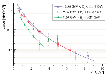
The proximity of the GlueX data to the threshold allows us to extrapolate the differential cross sections both in beam energy and outside of the physical region and estimate the forward cross section at threshold, . The forward cross section close to threshold, , enters in many theoretical models and plays an important role in understanding the photoproduction and the -proton interaction Kharzeev et al. (1999); Gryniuk and Vanderhaeghen (2016); Strakovsky et al. (2020); Pentchev and Strakovsky (2021). The dependence of the differential cross section can be related to the gluonic form factor of the proton, which is usually parametrized with a dipole function, Frankfurt and Strikman (2002); Mamo and Zahed (2020); Tong et al. (2021); Shanahan and Detmold (2019). In Fig. 15 we show the results of fits to the measured differential cross sections with squared dipole functions of the form , excluding the high- region in the lowest energy region. The results of the fits are summarized in Table 2.
| [GeV] | |||
|---|---|---|---|
| [GeV] | |||
| [nb/GeV2] | |||
| [GeV] | |||
The -slope is defined by the mass scale parameter, , and the fit results for are generally in good agreement with the lattice calculations Shanahan and Detmold (2019) of the gluon form factor that find GeV. More precisely, such agreement of the data (also in agreement with our data, Fig. 14) with the lattice calculations was demonstrated in Ref. Duran et al. (2023) using the holographic model of Ref. Mamo and Zahed (2021a).
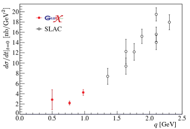
The fits in Fig. 15 also directly give an extrapolation of the cross sections to , , Table 2. These results are plotted in Fig. 16 as a function of the final proton (or ) c.m. momentum, , together with the SLAC measurements of at also extrapolated to using their measured exponential slope of GeV-2 Camerini et al. (1975). Such a plot allows extrapolation of to the threshold, , that corresponds to . Ref. Gryniuk and Vanderhaeghen (2016) uses the VMD model and dispersion relations to parametrize the forward scattering amplitude, , and to fit all existing photoproduction data including those data taken at large center-of-mass energies. The parametrization is then used to fit the forward differential cross sections and estimate - see Fig. 3 in Ref. Gryniuk and Vanderhaeghen (2016), which is an analog to our Fig. 16. Alternatively, the extrapolation to threshold can be done by expanding in partial waves, with the S-wave being dominant near threshold. Initial extrapolations were previously reported along with the preliminary GlueX results Pentchev , but will not be discussed further in this paper. It is of importance that the GlueX measurements are much closer to the threshold than the SLAC measurements Camerini et al. (1975) (the latter used in Ref. Gryniuk and Vanderhaeghen (2016)), at the same time constraining to lower values than the SLAC results and Ref. Gryniuk and Vanderhaeghen (2016). For the purpose of providing a quantitative estimate, let us assume is close in value and uncertainty to the lowest- data point in Fig. 16, nb/GeV2, where we have included the overall scale uncertainty.
This value corresponds to a very small scattering length, , which is given by Pentchev and Strakovsky (2021):
| (10) |
where is the c.m. momenta of the initial particles and is the photon- coupling constant obtained from the decay width. We find fm, which, compared to the size of the proton of fm scale, indicates a very weak interaction. However, note that the VMD model is used in Eq.(10) to extract this value.
We can use the mass scale from the fits in Fig. 15 (Table 2) to estimate the proton mass radius as prescribed in Ref. Kharzeev (2021),
| (11) |
where the scalar gravitational form factor, , is related to the measured -distributions through the VMD model. Eq.(11) gives fm, fm, and fm for , , and GeV, respectively. More sophisticated estimations of the proton mass radius require knowledge of the and gravitational form factors separately Guo et al. (2021), Duran et al. (2023).

In Fig. 17 we compare our total cross section results to models that assume factorization of the photoproduction into a hard quark-gluon interaction and the GPDs describing the partonic distributions of the proton. This factorization in exclusive heavy-meson photoproduction in terms of GPDs was studied in the kinematic region of low and high beam energies Ivanov et al. (2004). The factorization was explicitly demonstrated by direct leading order (LO) and next-to-leading order (NLO) calculations. In Ref. Guo et al. (2021), it was shown that in the limit of high meson masses and at LO, the factorization in terms of gluon GPDs is still valid down to the threshold. Calculations in this framework were performed for the photoproduction cross section using parametrizations of the gravitational form factors obtained from the lattice results of Ref. Shanahan and Detmold (2019). These calculations for the total cross section are compared to our measurements in Fig. 17. While they agree better with the SLAC data at higher energies, they underestimate our near-threshold measurements. Recently, the authors of Ref. Ivanov et al. (2004) extended their calculations to the threshold region at LO Ivanov et al. (2022). These calculations, plotted also in Fig. 17, are in a very good agreement with the total cross section measurements. Attempts to include the NLO contribution result in large uncertainties due to the poor knowledge of the corresponding GPD functions in this kinematic region Sznajder and Wagner (2022). This indicates that our measurements can strongly constrain the relevant gluon GPD functions.
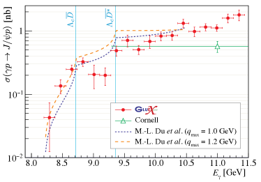
The authors of Ref. Du et al. (2020) propose an alternative mechanism of photoproduction with a dominant exchange of open-charm channels and in box diagrams. We show the total cross section results of this model in Fig. 18, and find good qualitative agreement with our measurements. In particular, in the data we see structures peaking at both the and thresholds that can be interpreted as the cusps expected with this reaction mechanism. However, the exchange of heavy hadrons in this model implies a very shallow -dependence in the differential cross sections. This is not supported by the steeply falling cross sections we observe, as shown in Fig. 15. Therefore, our differential cross section measurements do not support a dominant contribution from these open charm exchanges, although the enhancement at high observed for the lowest beam energy region is consistent with a possible contribution from these exchanges. Alternatively, in Ref. Pire et al. (2022) it was shown that the high- enhancement can be explained by -channel contribution assuming factorization in terms of Transition Distribution Amplitudes Pire et al. (2021).
In Ref. Winney et al. (2023), the model-independent effective range expansion was used to parameterize the lowest partial waves. Fits to the total and differential cross sections from this paper and from Ref. Duran et al. (2023) show that the expansion is rapidly convergent, with the waves saturating the forward peak in the measured photon energy range. Furthermore, the energy dependence of the total cross section near the open-charm thresholds was shown to be consistent with the appearance of intermediate states, as suggested by Ref. Du et al. (2020).
It is important to be able to understand the dynamics underlying photoproduction at threshold, and possibly to identify a kinematic region that can be used to extract the proton gluonic form factors. Based on the -slopes of the differential cross sections (Fig. 15) and also the results of Ref. Duran et al. (2023), the differential cross section at low -values is consistent with being dominantly due to gluonic exchange. However, the possible structures in the total cross section energy dependence and the flattening of the differential cross section near threshold are consistent with contributions from open-charm intermediate states. So far, from the analyses of Ref. Winney et al. (2023) it is not possible to distinguish between the gluon and open-charm exchange mechanisms. Certainly, further theoretical work is needed to understand the mechanism of near-threshold production and its relation to the gluonic structure of the proton, especially since hints of open charm production are visible. On the experimental side, higher statistics are needed to confirm the structures in the total cross section and the enhancement in the -dependence, the statistical significance of which at present does not allow making of definitive conclusions.
Acknowledgements.
We would like to thank A. N. H. Blin, A. Pilloni, A. P. Szczepaniak, and D. Winney for the fruitful discussions of the interpretation of the results. We would like to acknowledge the outstanding efforts of the staff of the Accelerator and the Physics Divisions at Jefferson Lab that made the experiment possible. This work was supported in part by the U.S. Department of Energy, the U.S. National Science Foundation, the German Research Foundation, Forschungszentrum Jülich GmbH, GSI Helmholtzzentrum für Schwerionenforschung GmbH, the Natural Sciences and Engineering Research Council of Canada, the Russian Foundation for Basic Research, the UK Science and Technology Facilities Council, the Chilean Comisión Nacional de Investigación Científica y Tecnológica, the National Natural Science Foundation of China and the China Scholarship Council. This material is based upon work supported by the U.S. Department of Energy, Office of Science, Office of Nuclear Physics under contract DE-AC0506OR23177. This research used resources of the National Energy Research Scientific Computing Center (NERSC), a U.S. Department of Energy Office of Science User Facility operated under Contract No. DE-AC02-05CH11231. This work used the Extreme Science and Engineering Discovery Environment (XSEDE), which is supported by National Science Foundation grant number ACI-1548562. Specifically, it used the Bridges system, which is supported by NSF award number ACI-1445606, at the Pittsburgh Supercomputing Center (PSC).Appendix A Numerical results
| Energy bin [GeV] | [nb] |
|---|---|
| bin | |||
|---|---|---|---|
| [GeV2] | [GeV2] | [GeV] | |
| 0.92 | 9.14 | ||
| 1.25 | 8.96 | ||
| 1.72 | 8.80 | ||
| 2.24 | 8.77 | ||
| 2.94 | 8.78 | ||
| 3.92 | 8.95 | ||
| 4.95 | 9.10 |
| bin | |||
|---|---|---|---|
| [GeV2] | [GeV2] | [GeV] | |
| 0.69 | 10.00 | ||
| 0.87 | 9.85 | ||
| 1.21 | 9.83 | ||
| 1.71 | 9.83 | ||
| 2.24 | 9.82 | ||
| 2.97 | 9.84 | ||
| 3.89 | 9.86 | ||
| 5.06 | 9.76 | ||
| 6.37 | 9.93 |
| bin | |||
|---|---|---|---|
| [GeV2] | [GeV2] | [GeV] | |
| 0.46 | 10.96 | ||
| 0.60 | 10.87 | ||
| 0.88 | 10.85 | ||
| 1.18 | 10.86 | ||
| 1.69 | 10.86 | ||
| 2.24 | 10.83 | ||
| 2.87 | 10.82 | ||
| 3.92 | 10.81 | ||
| 4.93 | 10.78 | ||
| 6.97 | 10.70 | ||
| 8.36 | 10.70 |
References
- Ali et al. (2019) (GlueX collaboration) A. Ali et al. (GlueX collaboration), Phys. Rev. Lett. 123, 072001 (2019).
- Frankfurt and Strikman (2002) L. Frankfurt and M. Strikman, Phys. Rev. D 66, 031502 (2002).
- Kharzeev et al. (1999) D. Kharzeev, H. Satz, A. Syamtomov, and G. Zinovev, Nucl.Phys. A 661, 568 (1999).
- Hatta and Yang (2018) Y. Hatta and D.-L. Yang, Phys. Rev. D 98 (2018), 10.1103/physrevd.98.074003.
- Kou et al. (2021) W. Kou, R. Wang, and X. Chen, “Determination of the gluonic d-term and mechanical radii of proton from experimental data,” (2021), arXiv:2104.12962 [hep-ph] .
- Strakovsky et al. (2020) I. I. Strakovsky, D. Epifanov, and L. Pentchev, Phys. Rev. C 101 (2020), 10.1103/physrevc.101.042201.
- Pentchev and Strakovsky (2021) L. Pentchev and I. I. Strakovsky, Eur.Phys.J.A 57 (2021), 10.1140/epja/s10050-021-00364-4.
- Ivanov et al. (2004) D. Y. Ivanov, A. Schafer, L. Szymanowski, and G. Krasnikov, Eur. Phys. J. C 34, 297 (2004), [Erratum: Eur.Phys.J.C 75, 75 (2015)], arXiv:hep-ph/0401131 .
- Hatta and Strikman (2021) Y. Hatta and M. Strikman, Phys. Lett. B 817, 136295 (2021).
- Guo et al. (2021) Y. Guo, X. Ji, and Y. Liu, Phys. Rev. D 103, 096010 (2021), arXiv:2103.11506 [hep-ph] .
- Kharzeev (2021) D. E. Kharzeev, Physical Review D 104 (2021), 10.1103/physrevd.104.054015.
- Ji et al. (2021) X. Ji, Y. Liu, and I. Zahed, Phys. Rev. D 103 (2021), 10.1103/physrevd.103.074002.
- Mamo and Zahed (2021a) K. A. Mamo and I. Zahed, Phys. Rev. D 103 (2021a), 10.1103/physrevd.103.094010.
- Wang et al. (2021) R. Wang, W. Kou, Y.-P. Xie, and X. Chen, Phys. Rev. D 103, L091501 (2021).
- Hatta et al. (2019) Y. Hatta, A. Rajan, and D.-L. Yang, Phys. Rev. D 100 (2019), 10.1103/physrevd.100.014032.
- Mamo and Zahed (2020) K. A. Mamo and I. Zahed, Phys. Rev. D 101 (2020), 10.1103/physrevd.101.086003.
- Mamo and Zahed (2021b) K. A. Mamo and I. Zahed, Physical Review D 104 (2021b), 10.1103/physrevd.104.066023.
- Sun et al. (2022) P. Sun, X.-B. Tong, and F. Yuan, Phys. Rev. D 105 (2022), 10.1103/physrevd.105.054032.
- Du et al. (2020) M.-L. Du, V. Baru, F.-K. Guo, C. Hanhart, U.-G. Meißner, A. Nefediev, and I. Strakovsky, Eur.Phys.J.C 80 (2020), 10.1140/epjc/s10052-020-08620-5.
- Aaij et al. (2015) R. Aaij et al. (LHCb Collaboration), Phys. Rev. Lett. 115, 072001 (2015).
- Aaij et al. (2019) R. Aaij et al. (LHCb Collaboration), Phys. Rev. Lett. 122, 222001 (2019).
- Wang et al. (2015) Q. Wang, X.-H. Liu, and Q. Zhao, Phys. Rev. D 92, 034022 (2015).
- Kubarovsky and Voloshin (2015) V. Kubarovsky and M. B. Voloshin, Phys. Rev. D 92, 031502 (2015).
- Karliner and Rosner (2016) M. Karliner and J. Rosner, Phys. Lett. B 752, 329 (2016).
- Blin et al. (2016) A. Blin, C. Fernandez - Ramirez, A. Jackura, V. Mathieu, V. Mokeev, A. Pilloni, and A. Szczepaniak, Phys. Rev. D 94, 034002 (2016).
- Adhikari et al. (2021) S. Adhikari, C. Akondi, H. Al Ghoul, A. Ali, M. Amaryan, E. Anassontzis, A. Austregesilo, F. Barbosa, J. Barlow, A. Barnes, and et al., Nucl. Instrum. Meth. A 987, 164807 (2021).
- Barbosa et al. (2015) F. Barbosa, C. Hutton, A. Sitnikov, A. Somov, S. Somov, and I. Tolstukhin, Nucl. Instrum. Meth. A 795, 376 (2015).
- Pooser et al. (2019) E. Pooser, F. Barbosa, W. Boeglin, C. Hutton, M. Ito, M. Kamel, P. K. A. LLodra, N. Sandoval, S. Taylor, T. Whitlatch, S. Worthington, C. Yero, and B. Zihlmann, Nucl. Instrum. Meth. A 927, 330 (2019).
- Jarvis et al. (2020) N. Jarvis, C. Meyer, B. Zihlmann, M. Staib, A. Austregesilo, F. Barbosa, C. Dickover, V. Razmyslovich, S. Taylor, Y. Van Haarlem, et al., Nucl. Instrum. Meth. A 962, 163727 (2020).
- Pentchev et al. (2017) L. Pentchev, F. Barbosa, V. Berdnikov, D. Butler, S. Furletov, L. Robison, and B. Zihlmann, Nucl. Instrum. Meth. A 845, 281 (2017).
- Beattie et al. (2018) T. D. Beattie, A. M. Foda, C. L. Henschel, S. Katsaganis, S. T. Krueger, G. J. Lolos, Z. Papandreou, et al., Nucl. Instrum. Meth. A 896, 24 (2018).
- Paremuzyan (2017) R. Paremuzyan, (private communication) (2017).
- Berger et al. (2002) E. Berger, M. Diehl, and B. Pire, Eur.Phys.J.C 23, 675 (2002).
- Borah et al. (2020) K. Borah, R. J. Hill, G. Lee, and O. Tomalak, Phys. Rev. D 102 (2020), 10.1103/physrevd.102.074012.
- Allison et al. (2016) J. Allison et al., Nucl. Instrum. Meth. A 835, 186 (2016).
- (36) W. Verkerke and D. Kirkby, https://root.cern/download/doc/RooFit_Users_Manual_2.91-33.pdf.
- Tanabashi et al. (2018) (Particle Data Group) M. Tanabashi et al. (Particle Data Group), Phys. Rev. D 98, 030001 (2018).
- Heller et al. (2018) M. Heller, O. Tomalak, and M. Vanderhaeghen, Phys. Rev. D 97, 076012 (2018).
- Boer (2019) M. Boer, Jefferson Lab, Hall C public note no. 1000 (2019).
- Boer et al. (2015) M. Boer, M. Guidal, and M. Vanderhaeghen, Eur.Phys.J.A 51, 103 (2015).
- Duran et al. (2023) B. Duran, Z.-E. Meziani, S. Joosten, M. K. Jones, S. Prasad, C. Peng, W. Armstrong, H. Atac, E. Chudakov, H. Bhatt, D. Bhetuwal, M. Boer, A. Camsonne, J.-P. Chen, M. M. Dalton, N. Deokar, M. Diefenthaler, J. Dunne, L. El Fassi, E. Fuchey, H. Gao, D. Gaskell, O. Hansen, F. Hauenstein, D. Higinbotham, S. Jia, A. Karki, C. Keppel, P. King, H. S. Ko, X. Li, R. Li, D. Mack, S. Malace, M. McCaughan, R. E. McClellan, R. Michaels, D. Meekins, M. Paolone, L. Pentchev, E. Pooser, A. Puckett, R. Radloff, M. Rehfuss, P. E. Reimer, S. Riordan, B. Sawatzky, A. Smith, N. Sparveris, H. Szumila-Vance, S. Wood, J. Xie, Z. Ye, C. Yero, and Z. Zhao, Nature 615, 813 (2023).
- Gryniuk and Vanderhaeghen (2016) O. Gryniuk and M. Vanderhaeghen, Phys. Rev. D 94, 074001 (2016).
- Tong et al. (2021) X.-B. Tong, J.-P. Ma, and F. Yuan, “Gluon gravitational form factors at large momentum transfer,” (2021), arXiv:2101.02395 [hep-ph] .
- Shanahan and Detmold (2019) P. E. Shanahan and W. Detmold, Phys. Rev. D 99, 014511 (2019), arXiv:1810.04626 [hep-lat] .
- Camerini et al. (1975) U. Camerini, J. Learned, R. Prepost, C. Spencer, D. Wiser, W. Ash, R. L. Anderson, D. M. Ritson, D. Sherden, and C. K. Sinclair, Phys. Rev. Lett. 35, 483 (1975).
- (46) L. Pentchev, https://indico.jlab.org/event/344/contributions/10353/attachments/8401/12067/LPentchev_Jpsi_QNP2022.pdf.
- Gittelman et al. (1975) B. Gittelman, K. M. Hanson, D. Larson, E. Loh, A. Silverman, and G. Theodosiou, Phys. Rev. Lett. 35, 1616 (1975).
- Ivanov et al. (2022) D. Ivanov, P. Sznajder, L. Szymanowski, and J. Wagner, (private communication) (2022).
- Sznajder and Wagner (2022) P. Sznajder and J. Wagner, (private communication) (2022).
- Pire et al. (2022) B. Pire, K. M. Semenov-Tian-Shansky, A. A. Shaikhutdinova, and L. Szymanowski, “Pion and photon beam initiated backward charmonium or lepton pair production,” (2022).
- Pire et al. (2021) B. Pire, K. Semenov-Tian-Shansky, and L. Szymanowski, Phys. Rep. 940, 1 (2021).
- Winney et al. (2023) D. Winney, C. Fernandez-Ramirez, A. Pilloni, A. N. H. Blin, M. Albaladejo, L. Bibrzycki, N. Hammoud, J. Liao, V. Mathieu, G. Montana, R. J. Perry, V. Shastry, W. A. Smith, and A. P. Szczepaniak, “Dynamics in near-threshold photoproduction,” (2023), arXiv:2305.01449 [hep-ph] .