ASAS-SN Sky Patrol v2.0

Abstract

The All-Sky Automated Survey for Supernovae (ASAS-SN) began observing in late-2011 and has been imaging the entire sky with nightly cadence since late 2017. A core goal of ASAS-SN is to release as much useful data as possible to the community. Working towards this goal, in 2017 the first ASAS-SN Sky Patrol was established as a tool for the community to obtain light curves from our data with no preselection of targets. Then, in 2020 we released static $V$-band photometry from 2013–2018 for $\sim 61$ million sources. Here we describe the next generation ASAS-SN Sky Patrol, Version 2.0, which represents a major progression of this effort. Sky Patrol 2.0 provides continuously updated light curves for $\sim 111$ million targets derived from numerous external catalogs of stars, galaxies, and solar system objects. We are generally able to serve photometry data within an hour of observation. Moreover, with a novel database architecture, the catalogs and light curves can be queried at unparalleled speed, returning thousands of light curves within seconds. Light curves can be accessed through a web interface (http://asas-sn.ifa.hawaii.edu/skypatrol/) or a Python client (https://asas-sn.ifa.hawaii.edu/documentation). The Python client can be used to retrieve up to 1 million light curves, generally limited only by bandwidth. This paper gives an updated overview of our survey, introduces the new Sky Patrol, and describes its system architecture. These results provide significant new capabilities to the community for pursuing multi-messenger and time-domain astronomy.

1. Introduction

The All-Sky Automated Survey for Supernovae (ASAS-SN; Shappee et al., 2014; Kochanek et al., 2017a) began observing in 2011 with the mission of identifying bright transients across the whole sky with minimal observational bias. With its initial two-camera station at the Haleakala Observatory (Hawaii), ASAS-SN was able to image the visible sky roughly once every 5 days. By late 2013, our team had installed two additional cameras on the Haleakala station, by April 2014 we had installed another two-camera station at the Cerro Tololo International Obervatory (CTIO, Chile), and by mid-2015 we had installed two more cameras at the CTIO station. These additional cameras increased our survey cadence and allowed us to image the entire sky every few nights. In late 2017, we added three additional 4-camera stations, one at McDonald Observatory (Texas), one at the South African Astrophysical Observatory (SAAO, South Africa), and an additional station at CTIO. This geographic redundancy in both the northern and southern hemispheres ensures that we are able to observe the entire sky on a nightly basis. Our stations are hosted by the Las Cumbres Observatory Global Telescope Network (LCOGT; Brown et al., 2013) and we have the ability to download and reduce images within minutes of their exposures.

ASAS-SN units use cooled, back-illuminated FLI ProLine $2K\times 2K$ CCD cameras with 14-cm aperture Nikon telephoto lenses. The units’ field-of-view is 4.47 degrees on a side (20 degrees²) with a pixel size of 8.0 arcsec. Ideally, each observation epoch consists of three dithered 90 second exposures, though we are currently averaging 2.7 exposures per epoch due to scheduling and weather events. The two original units used $V$-band filters until late 2018, after which we switched to $g$-band filters. The three newer units have used $g$-band filters from the start. The limiting $V$-band and $g$-band magnitudes are $m\sim 17.5$ and $m\sim 18.5$, respectively.

In June 2017, we launched Sky Patrol V1.0; https://asas-sn.osu.edu/. The goal of Sky Patrol V1.0 was to allow users to request light curves from our image archive. Rather than pre-computing light curves for a set number of targets, Sky Patrol V1.0 provides uncensored light curves for any user-specified coordinates. Aperture photometry is performed in real time at the user’s requested coordinates using local, nearby stars to calibrate the photometry. Though the flexibility of that tool is admirable, its need to compute light curves in real time restricts both the size and frequency of users’ queries.

To partially alleviate these limitations, we pre-computed static $V$-band light curves and released the ASAS-SN Catalog of Variable Stars (https://asas-sn.osu.edu/variables; Jayasinghe et al., 2018, 2019b, 2019a). We then expanded these catalogs to include 61.5 million stars across the sky used in the variable star search (https://asas-sn.osu.edu/photometry; Jayasinghe et al., 2019c). We have also created a citizen science program using the Zooniverse platform named Citizen ASAS-SN (Christy et al. 2021, 2022b) where, as of Jan 1 2023, $\sim 5,300$ volunteers have classified over 1,400,000 ASAS-SN $g$-band light curves through searches for unusual variable stars.

Finally, in September 2021, we further expanded Sky Patrol V1.0 to not only perform forced-aperture photometry on our reduced images but also to enable users to run aperture photometry on the coadded, image-subtracted data for each epoch with or without the flux of the source on the reference image added.

This paper outlines Sky Patrol V2.0, which seeks to maintain the flexibility of its predecessor (which remains available) while massively improving on it in both speed and scale. V2.0 not only serves pre-computed light curves for a select list of $\sim 111$ million targets, but it also continuously updates the light curves in real time. Like Sky Patrol V1.0, they are uncensored light curves with no deliberate delays in the updates. To do this, we have built a system on top of our automated image processing pipeline that performs photometry and updates our public database as new observations are obtained, calibrated, and reduced.

In §2, we describe our imaging pipeline and a number of science products resulting from our survey. In §3, we discuss our collated target list, their catalogs of origin, and how they can be queried. In §4, we introduce the Python and web interfaces to our dataset, and provide several usage examples.In §5, we discuss the photometric properties and precision of this survey tool. In §6, we discuss the design and metrics of our database. In §7, we give a short summary and explore the applications of this tool in upcoming research.

2. Survey Overview

To date, our high-cadence network of telescopes has produced millions of images. By repeatedly conducting observations in an all-sky fixed grid, we are able to leverage deeply stacked reference images to perform high-precision photometry and optical analysis for a number of different science cases. This section describes our imaging and photometry pipeline, as well as a variety of notable science products resulting from our survey’s data.

2.1. Photometry

To achieve full coverage of the sky the ASAS-SN observations are scheduled on 2,824 tessellated fields. Each field matches the 20 degree² camera field-of-view and has at least a 0.5 degree overlap with adjacent fields. The fields are divided into 706 pointings, where each of the 4 cameras in an ASAS-SN unit observes a specific field. Figure 1 shows the our field map and the number of images taken for each field up to the time of writing.

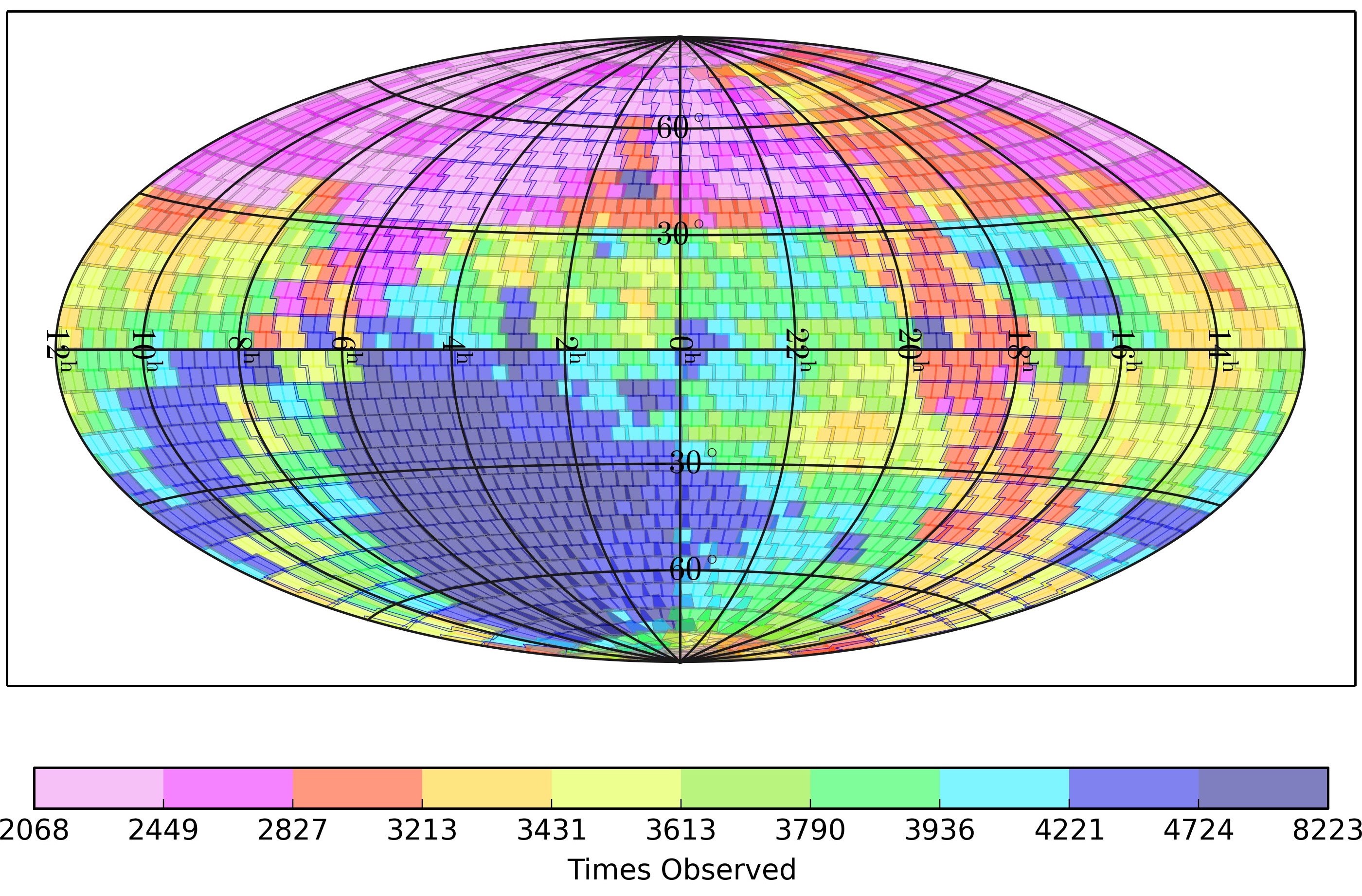
Figure 1.— Equatorial projection of ASAS-SN fields and number of images taken as of Feb 25, 2023. There are, on average, $2.7$ images for each epoch.

The data are analysed using a fully-automated pipeline based on the ISIS image-subtraction package (Alard & Lupton, 1998; Alard, 2000). Each photometric epoch (usually) combines three dithered 90-second image exposures with a 4.47$\times$4.47 degree field-of-view of the field that is subtracted from a reference image. Typically, within an hour of observation our pipeline reduces and co-adds the subtracted images together into observation epochs. We then perform photometry on each of these co-added subtractions and the reference image.

The reference images are calibrated using isolated stars from the ATLAS Reference Catalog (Tonry et al., 2018) and by fitting a 2D polynomial to find the zero point as a function of XY position on each reference image. This step reduces any leftover zeropoint issues not removed by flat fielding. After calibration, we perform photometry on the reference image using IRAF apphot with a fixed aperture of 2 pixels, or approximately 16 arcsec, radius and a background annulus spanning 7–10 pixels in radius. We perform photometry on all targets from our input catalogs that fall within each field and are more than 0.2 degrees away from the image boundaries. We then use apphot on the same apertures to perform photometry on each subtracted image, generating a differential light curve to which the reference flux is added. Finally, the photometry for each target in a given co-add is appended to the corresponding light curves in our database.

For each epoch in a given light curve, we record the Julian date, camera filter, FWHM, measured flux, flux error, magnitude, magnitude error, and 5 $\sigma{}$ limiting magnitude. For any epoch where the source is not detected at 5 $\sigma{}$, we still give the forced aperture flux but report the limiting magnitude instead of the magnitude and record the magnitude error as 99.99.

Typically, we publish new photometric measurements within an hour of observation. On the timescale of a day, images are reviewed either manually or by additional quality checks for cirrus, clouds, or other image quality issues. Images are then determined to be either "good" or "bad." When this occurs, the corresponding photometry is then flagged as such in the Sky Patrol V2.0 database. We advise caution when using and interpreting photometry that has not been flagged as "good."

Because we are constantly appending new observations to our light curves and periodically rebuilding reference images—which triggers our pipeline to re-run all photometry on previous co-adds—our light curves are consistently growing in length and improving in quality.

2.2. Science Products

The ASAS-SN survey was initially designed to create a local census of nearby, bright extra galactic transients and has been used to discover and study supernovae (e.g., Shappee et al., 2016; Holoien et al., 2016a, 2017c, 2017b, 2017a, 2017d; Kochanek et al., 2017b; Bose et al., 2019; Brown et al., 2019; Holoien et al., 2019b; Shappee et al., 2019a; Vallely et al., 2019; Neumann et al., 2022; Desai et al. in prep.), superluminous supernovae (e.g., Dong et al., 2016; Godoy-Rivera et al., 2017; Bose et al., 2018), rapidly evolving blue transients (e.g., Prentice et al., 2018), tidal disruption events (TDEs; e.g., Holoien et al., 2014a, 2016a, 2016b; Holoien et al., 2018; Holoien et al., 2019c, a, 2020; Brown et al., 2016; Brown et al., 2018; Hinkle et al., 2020, 2021b, 2021a), ambiguous nuclear transients (ANTs; e.g., Neustadt et al., 2020; Hinkle et al., 2021a; Holoien et al., 2022; Hinkle et al., 2022a), active galactic nuclei variability (e.g., Yuk et al., 2022), orphan blazar flares (de Jaeger et al., 2022a), large outbursts from active galactic nuclei (e.g., Shappee et al., 2014; Trakhtenbrot et al., 2019; Hinkle et al., 2022b; Neustadt et al., 2022), changing-look blazars (e.g., Mishra et al., 2021), and even a potential repeating partial TDE (e.g., Payne et al., 2021; Tucker et al., 2021; Payne et al., 2022a, b). ASAS-SN has also been used to search for optical counterparts for multi-messenger events such as high-energy neutrinos observed by Icecube (e.g., Icecube Collaboration et al., 2017; Garrappa et al., 2019; IceCube Collaboration et al., 2018; Franckowiak et al., 2020; Necker et al., 2022) and LIGO/VIRGO gravitational wave events (e.g., Abbott et al., 2020; Shappee et al., 2019b, c, d; de Jaeger et al., 2022b).

Moreover, the ASAS-SN data have been used in hundreds of publications to study Galactic and solar system objects. This includes large variable star studies (Jayasinghe et al., 2018, 2019b, 2019a; Pawlak et al., 2019; Jayasinghe et al., 2019c; O’Grady et al., 2020; Jayasinghe et al., 2021; Rowan et al., 2021; Christy et al., 2022b, a), deriving period–luminosity relationships for $\delta$ Scuti stars (Jayasinghe et al., 2020b), fitting detached eclipsing binaries parameters (Way et al., 2022; Rowan et al., 2022a, b), studying contact binaries (Jayasinghe et al., 2020a), observing accreting white dwarf systems (e.g., Campbell et al., 2015; Littlefield et al., 2016), studying young stellar object variability (e.g., Holoien et al., 2014b; Herczeg et al., 2016; Rodriguez et al., 2016; Sicilia-Aguilar et al., 2017; Gully-Santiago et al., 2017; Osborn et al., 2017; Rodriguez et al., 2017; Bredall et al., 2020). Furthermore, ASAS-SN was used to examine the long-term variability of Boyajian’s Star (Simon et al., 2018) and has even recently identified a potential new "Boyajian’s Star" analog (the source has been nicknamed Zachy’s Star), exhibiting similar rapid dimming events (Way et al., 2019). ASAS-SN data have also been used to identify M-dwarf flares (e.g., Schmidt et al., 2014, 2016, 2019; Rodríguez Martínez et al., 2020; Zeldes et al., 2021), Novae and CVs (e.g., Kato et al., 2014a; Kato et al., 2014b; Kato et al., 2016, 2017; Li et al., 2017; Aydi et al., 2019, 2020a; Aydi et al., 2020b; Kato et al., 2020; Kawash et al., 2021a, b, 2022), X-ray binaries (e.g., Tucker et al., 2018), and R Coronae Borealis stars (e.g., Shields et al., 2019). ASAS-SN data have also been used to study stars and exoplanets by observing microlensing events (e.g., Dong et al., 2019; Wyrzykowski et al., 2020), determining asteroseismic distances for M giants (e.g., Auge et al., 2020), deriving gyrochronologic ages for exoplanet host stars (e.g., Gilbert et al., 2020), and vetting exoplanet candidates for background eclipsing binaries (e.g., Rodriguez et al., 2019). Finally, ASAS-SN data have even been useful for solar system studies through asteroid shape modeling (e.g., Hanuš et al., 2020), discovering 2 new comets in outburst (Prieto et al., 2017; van Buitenen et al., 2018), and recovering the near-Earth asteroid 2019OK (Jacques et al., 2019).

These studies demonstrate the wide utility of the ASAS-SN network and its dataset and why we have created a variety of tools which the community can benefit from.

3. Input Catalogs

Unlike ASAS-SN Sky Patrol V1.0, which allowed users to request light curves at arbitrary points on the sky, Sky Patrol V2.0 by construction only serves pre-computed light curves for objects in our input catalogs. Our input catalogs consist of stellar sources, external catalog sources, and solar system sources. Objects in our stellar source table and catalog source tables have all been cross-matched to a precision of 2 arcseconds and given unique ASAS-SN Sky Patrol Identifiers (asas_sn_id).

Source Catalog	Type	n sources
ASAS-SN Stellar Source Table	Stellar	98,602,587
Fermi LAT 10-Year Point Sources	Gamma Ray	5,788
Chandra Sources v2.0	X-Ray	317,224
Swift Master Catalog	Optical/UV/X-Ray/Gamma Ray	254,936
AllWISE AGN Catalog	Mid-IR/AGN	1,354,775
Million Optical/Radio/X-Ray Associations Catalog (MORX)	Optical/Radio/X-Ray	3,262,883
Million Quasars Catalog (MILLIQUAS)	QSO	1,979,676
Bright M-Dwarf All Sky Catalog	Stellar	8,927
AAVSO International Variable Star Index	Stellar	1,437,528
Galaxy List for the Advanced Detector Era (GLADE)	Galaxy	3,263,611

Table 1A breakdown of our input catalogs, with the numbers and types of sources included.

3.1. Stellar Sources

The stellar source table was constructed with the goal of providing an unbiased sample that maximizes the number of targets while maintaining the overall quality of our light curves. We used the ATLAS Reference Catalog (REFCAT2) to build the target list. Given the pixel size and magnitude sensitivity of our instruments, we chose to include objects with mean $g<18.5$ mag and where r1 $>20$ arcsec, where r1 is the radius where the cumulative flux exceeds that of the target star. Because REFCAT2 was compiled to include at least 99% of objects with $m\leq 19$ mag and curated to exclude non-stellar objects, this stellar source table should be considered an exhaustive list of all stars observable by ASAS-SN that are not heavily crowded.

Because REFCAT2 used Gaia Data Release 2 (Gaia DR2) for its astrometric solutions, we were able to directly match Gaia source IDs from the given RA and DEC coordinates. We then used the best-neighbour tables in the Gaia Archive to cross-match with AllWISE, SDSS, and 2MASS. Finally, we used the same Gaia source IDs to get TESS Input Catalog Version 8.0 (TIC) IDs. This means that users can query our stellar source table using either the original columns provided by REFCAT2 or by providing external catalog identifiers for any of these other cross-matched surveys.

We note that some of our external source catalog tables contain stellar objects that do not occur in the stellar table. However, given the completeness of REFCAT2, these objects typically fall outside our sensitivity or suffer from significant crowding.

3.2. Additional Catalog Sources

In addition to our stellar sources, Sky Patrol V2.0 provides light curves for a number of specialized catalogs from NASA’s High Energy Astrophysics Science Archive Research Center (HEASARC), as shown in Table 1. With the explicit goal of aiding multi-messenger astronomy we have included the entire source catalogs from Fermi LAT (Abdollahi et al., 2020), Chandra (Evans et al., 2010), and Swift (Nasa & Heasarc, 2018). For researchers interested in specific object and variable types we have included the AllWISE AGN catalog (Secrest et al., 2015), the Million Quasar Catalog (Milliquas; Flesch, 2021), the Brown Dwarf Catalog (Lépine & Gaidos, 2011), the AAVSO International Variable Star Index (Watson et al., 2006) and the Galaxy List for the Advanced Detector Era (GLADE; Dálya et al., 2018).

Whereas our stellar sources were selected from REFCAT2 to ensure detections given our magnitude limits, these catalogs were not pruned based on flux. Photometry is performed at all target coordinates in these catalogs without bias. As with the stellar sources, null detections will be timestamped and reported in our light curves with $\sigma\sim 99.99$. Our interface allows the user to query sources using all of the original columns of the input catalogs and, we have maintained the original naming conventions of the catalogs’ columns with few exceptions.

Because many sources appear in more than one of these catalogs and we have already done the cross-matching, users can perform JOIN operations on these tables using asas_sn_ids. In §5, we provide several examples of such queries in ADQL.

Finally, for a few of the catalogs, ASAS-SN spatial resolution is better than the accuracy of the catalog’s coordinates for some of its objects. In these cases, we make no effort to identify the corresponding optical counterpart and simply perform forced aperture photometry at the catalog’s reported coordinates with our normal aperture size. Thus, users must be cautious when using the ASAS-SN Sky Patrol V2.0 photometry for poorly localized sources. In these cases we recommend first searching for the corresponding optical counterpart’s photometry in Sky Patrol V2.0, and if not present, to use the slower Sky Patrol V1.0 to compute forced aperture photometry at the exact coordinates desired.

3.3. Solar System Sources

To provide photometry for asteroids and comets, we rely on updates from the Minor Planet Center Orbit Database (MPCORB Database) every 10 days. For each object in the most recent MPCORB Database relative to our observation, we calculate the position and run aperture photometry on all objects within that image. Unlike our other sources, we do not add flux from the reference images. Photometry on asteroids is run with the same aperture as our extra-solar sources, while comets are run in a different manner. Comet photometry is computed using 2–8 pixel apertures and a 15–20 pixel annulus. This means that each comet’s light curve will have 7 different magnitude values for each observation epoch. The goal of this regime is to provide researchers a detailed picture of the growth and decay of gas and dust tails as these comets traverse our solar system.

4. Interface

We have designed a simple, yet powerful interface for users to query objects from our input catalog tables and to seamlessly retrieve their corresponding light curves. This interface can be accessed through our Python client or our web portal. While these have similar functionality, queries on the web portal will have stricter limits on the number of sources returned in a single query. The web portal limits users to 10,000 sources per query, whereas the Python client allows up to 1 million sources per query. The latest version of the Python tool and documentation can be found at https://asas-sn.ifa.hawaii.edu/documentation. The web portal can be accessed at https://asas-sn.ifa.hawaii.edu/skypatrol.

ASAS-SN Sky Patrol light curves can be queried in a number of ways: cone searches, catalog IDs, random samples, and ADQL queries. Further statistical and plotting tools are also provided by the Python client. We detail the available methods of querying light curves below.

4.1. Cone Search

The cone search is the most basic operation that we allow. Users can provide RA, DEC, and a search radius, and obtain catalog entries and light curves for all sources within that cone. Our system is unique in that there is no limit on the radius of a cone search and that the speed of the query will not be affected by the size of the cone. Users can also filter the desired sources in their cone search by catalog. Moreover, our ADQL function set includes utilities for running cone searches in conjunction with more complex queries.

⬇

>>> 2ljm syasassn.tlient import SkyPatrolClient

>>> tlient = SkyPatrolClient()

>>> tlient.tjne_search(lf_deg=277.0,

97t_deg=-32.3,

lf9ius=e.0,

units=’fltmin’,

tftalog=’ffvsjvsx’)

fsas_sn_id lf_deg 97t_deg name

2920e90aea70 276.a466e -32.0330a GDS_J1827232

02643773a023 277.060ea -32.076e0 ASASSN-V J18

09e3070a7a90 2a0.42779 -30.0307e NSVS 367e363

… … … …

[6e94 ljws x 4 tjlumns]

4.2. Catalog IDs

Searching by catalog ID is the simplest way to access our data. To do this, the user can provide target IDs for any catalog that we have cross-matched against and our interface will return light curves for all the sources in our data that match that list. Our stellar source table can be queried with TESS, GAIA DR2, AllWISE, SDSS, REFCAT2, and 2MASS identifiers. Sources from the other catalogs can be queried directly by their survey identifiers (e.g., Swift, Chandra, or Fermi LAT).

⬇

>>> my_tic_ids = [66ea026, 467a009e, 3023a90]

>>> tlient.query_list(my_tic_ids,

tftalog=’st7llfl_mfin’,

id_col=’tit_i9’)

fsas_sn_id lf_deg 97t_deg tic_id

00920a324040 029.260077 -a.00ea64 3023a90

00e0076990a0 97.04e7e9 3a.234a0a 467a009e

00e007690703 a3.364422 3a.222347 66ea026

This utility is meant for users that already have a source list from a specific survey and that hope to use our light curves to supplement their research. This is also the fastest way to query our database.

4.3. Random Samples

This utility has been included for data scientists looking to train or test models on large unbiased samples of light curves. The random sample function allows users to pull arbitrary numbers of light curves along with their corresponding catalog data. The following example shows a random sample from the MORX catalog. This utility returns a new random sample each time. If users want to perform multiple experiments on the same random sample, they will need to save the returned asas_sn_ids.

⬇

>>> tlient.lfndom_sample(30000, tftalog="mjlx")

fsas_sn_id lf_deg 97t_deg name

66340360e0a9 04a.2a629 -a9.26900 IRAS 22436-

663403263663 209.09640 40.36277 SDSS J13562

77030e90739 007.00222 40.3600e MORX J20291

373a3360a93 2e7.67936 -a7.e02e0 TYCHO 9e00-

… … … …

[30000 ljws x 4 tjlumns]

4.4. ADQL Queries

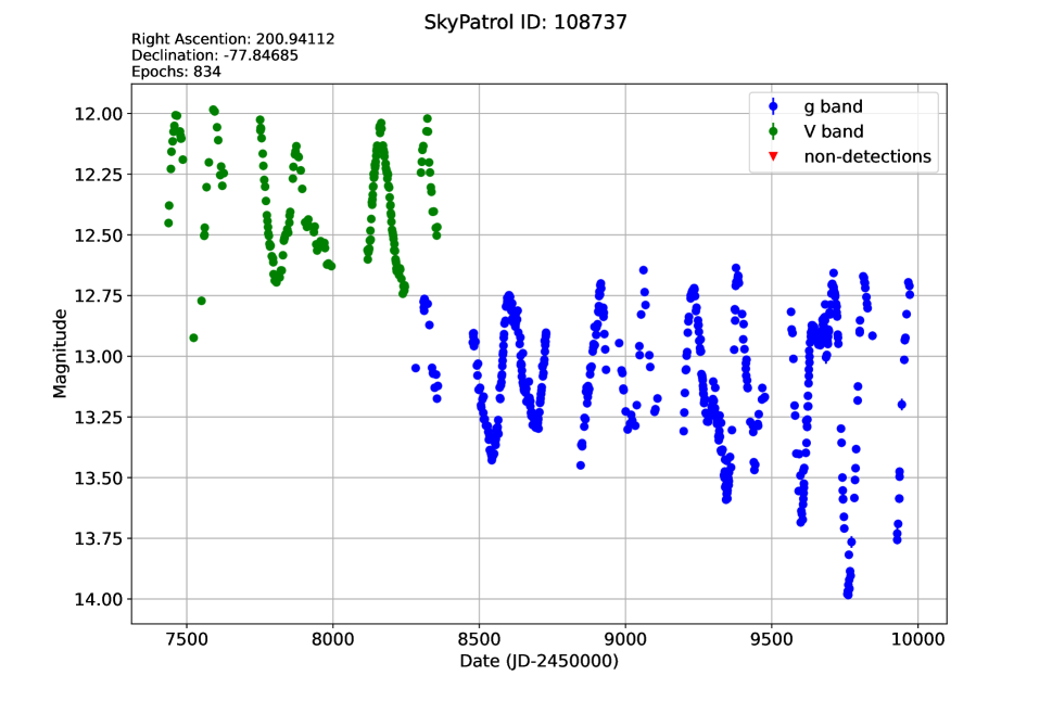
Figure 2.— Sample light curve generated by the Sky Patrol V2.0 Python client for the long-period variable star, BP Cha. The plot includes basic metadata as well as photometry for both g- and V-band filters.

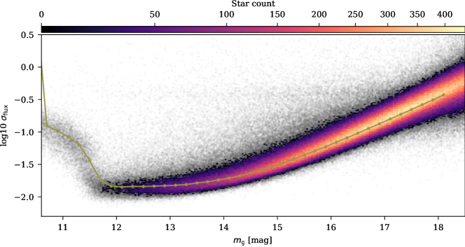
Figure 3.— Photometric precision of the $g$-band photometry as a function of Pan-STARRS $g$ magnitude. The dotted line represents the 50th percentile of the standard deviation of the flux in each bin. Note that saturation begins to set in around $g\sim 12$th mag.

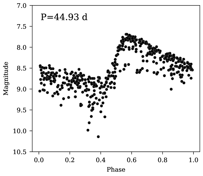
Figure 4.— Phased $g$ band light curve of the bright classical Cepheid SV Vul. Despite the extreme saturation, the photometry is still sufficiently clean for the periodicity to be measured.

While many other survey utilities, such as the Gaia DR2 Archive and VizieR, run interfaces compliant with the International Virtual Observatory Alliance’s (IVOA) Astronomical Data Query Language (ADQL) specification, we have chosen to use a custom grammar that both adds functionality and simplifies geometric queries.

In addition to the query functionality of traditional ADQL, we have included support for Common Table Expressions, WINDOW functions, correlated subqueries, and UNIONS. We have removed the common geometry functions such as BOX, CIRCLE, AREA, POINT, and CONTAINS. Instead of building predicates out of these functions, users can perform geometric searches either using the DISTANCE function or by specifying range conditions on RA and DEC. Below is an example cone search.

⬇

>>> query = """

SELECT

fsfs_sn_i9, lf_97g, 97t_97g

FROM st7llfl_mfin

WHERE DISTANCE(lf_97g, 97t_97g, 270, -aa) <= ARCMIN(00)

"""

⬇

>>> tlient.f9ql_query(query)

fsas_sn_id lf_deg 97t_deg

3367069 262.6e479e -aa.00e20a

3367730 27e.4927aa -aa.00720a

373a33e4e03 273.70a674 -aa.26026e

… … …

[2023 ljws x 0 tjlumns]

Because our data is stored in decimal degrees, we have provided functions to enter coordinates in HMS and DMS formats as well as functions to give distance constants in minutes and seconds of arc. Furthermore, because our lookup tables are running on top of Apache Spark, users can also leverage all of the Spark SQL functions.

The ADQL interface can be queried at will and used as a tool for exploring our source catalogs without any requirement that the user downloads the corresponding light curves. The speed of our execution engine allows scientists to query data on multiple sources across our input catalogs. However, users interested in the light curves for these catalog sources must include asas_sn_id as a column name in order to download the light curves.

4.5. Light Curve Utilities

The Python client provides additional functionality for downloading and processing individual or collections of light curves.

4.5.1 Collections

Once the user has found a set of targets through any of the 4 catalog query functions, they can now download their light curves. The cone search, catalog id, random sample, and ADQL query functions all have a boolean download parameter. If set, then the query function will return a LightCurveCollection object. This object provides the user with aggregate statistics on the collected light curves.

⬇

# Wi97 fngl7 tjn7 s7fltt j2 tflg7ts n7fl tt7 sjl7

>>> lcs = tlient.tjne_search(’3a:e4:33.e’,

’-aa:02:ee.22’,

lf9ius=2.0,

units=’97g’,

9jwnload=True,

threads=a)

>>> lcs.stats()

fsas_sn_id mean_mag std_mag 7sjtts

440090 33.300092 0.2a9eaa 436

44027e 36.060747 0.329060 094

440276 3e.a26790 0.0972a4 432

… … … …

[00690 ljws x 4 tjlumns]

4.6. Individual Light Curves

Once the user has downloaded a collection, they can view the individual light curves, as well as their meta data, periodograms, and plotted light curves. Moreover, because light curve data is held in memory as a pandas DataFrame, they can easily be saved to disk in csv format. Individual curves are retrieved from the collection using their asas_sn_id.

⬇

>>> lightcurve = lcs[30a707]

>>> lightcurve.9fta

jd 2lux 2lux_err mag mag_err limit 2wtm

24ea6a0 3a.e0 0.30 30.20 0.02 37.09 3.4e

24e90e3 34.42 0.32 30.e0 0.03 36.a7 3.6e

24ea706 3a.e2 0.33 30.20 0.03 36.97 3.40

24e900a 3a.66 0.09 30.22 0.02 37.20 3.47

24ea92e 26.60 0.32 32.a0 0.00 36.9e 3.42

[a04 ljws x 32 tjlumns]

As well as providing the photometric data for each of our light curves. We also provide some basic functions, such as plotting, lomb-scargle, and period finding. Fig. 2 shows a sample plot for a long period variable star from the AAVSO catalog.

⬇

# Simsl7 Pljt

>>> lightcurve.slot(stjt_filter=’fll’)

# An Astljsy LjmbStflgl7 jbj7tt is flsj l7tuln79

>>> 2, s, ls = lightcurve.lomb_scargle()

>>> lightcurve.2ind_period(2)

3e2.0293aaa630ae0a

5. Photometric properties and examples

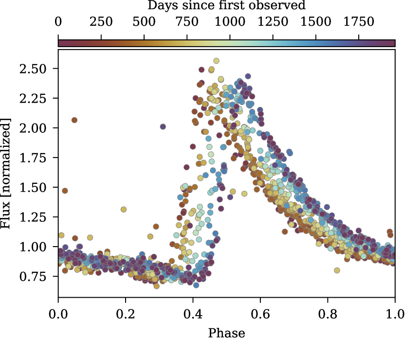
Figure 5.— Long period Blazhko modulation in the RR Lyrae variable CD Scl observed by ASAS-SN in $g$-band. The long baseline of g-band data allows for multiple cycles to be observed.

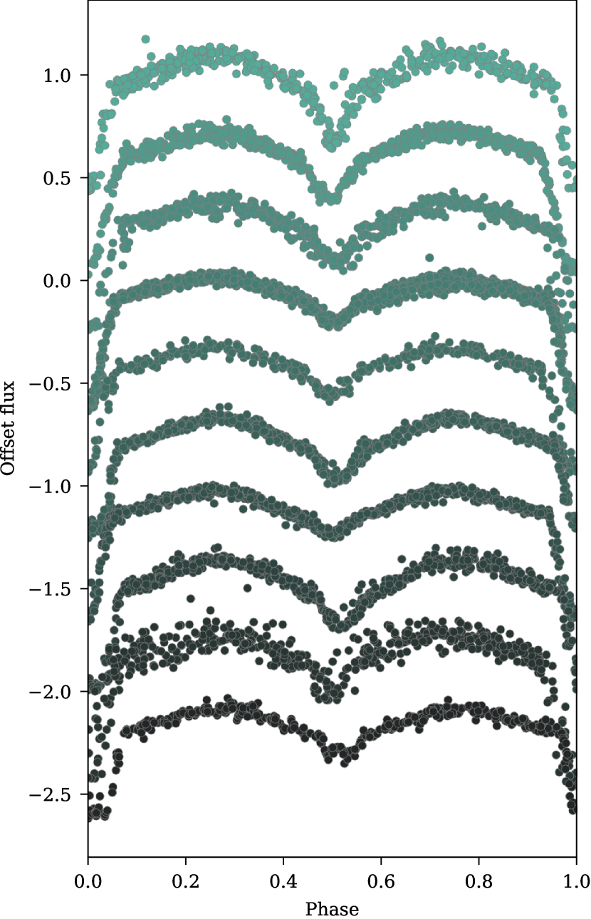
Figure 6.— A selection of several random eclipsing binaries with g-band photometry.

To demonstrate the photometric precision of the ASAS-SN $g$-band photometry, we downloaded 1,000,000 random light curves from the stellar_main catalogue, distributed over a range of Gaia DR2 magnitudes. For each light curve, we removed bad fluxes as indicated by the quality flags. We additionally normalized the flux of each camera to unity and perform a 5$\sigma$ clipping. We then measured the standard deviation of the entire light curve for each star. This metric is useful as a rough indication of the photometric precision for the source. We show the photometric precision of the $g$-band photometry as a function of Gaia magnitude in Fig. 3.

As seen in Fig. 3, saturation in $g$-band begins to set in around $g\sim 12.5$ mag with the photometric precision becoming significantly worse around $g\sim 11$ mag. At the time of this publication, we suggest using Sky Patrol V1.0 for significantly saturated ($g\mathrel{\hbox{\hbox to0.0pt{\hbox{\lower 4.0pt\hbox{$\sim$}}\hss}\hbox{$<$}}}11.5$ mag) targets to avoid the residuals that image subtraction creates for such sources. Future data releases we attempt to improve photometry for extremely saturated sources ($5\mathrel{\hbox{\hbox to0.0pt{\hbox{\lower 4.0pt\hbox{$\sim$}}\hss}\hbox{$<$}}}g\mathrel{\hbox{\hbox to0.0pt{\hbox{\lower 4.0pt\hbox{$\sim$}}\hss}\hbox{$<$}}}11.5$ mag).

We next illustrate the utility of ASAS-SN photometry with several non-transient variable sources. For each source, we use only the data returned by the query, with simple cuts on the quality flags as described above. Fig. 4 shows the photometry of SV Vul, a bright ($g\approx 8.2$ mag; Tonry et al., 2018) classical Cepheid variable. While there are clear outliers that are not accurately captured by the data quality flags, there is no issue in recovering the known periodicity of around 45 days despite its brightness.

Figure. 5 demonstrates the exceptional baseline provided by ASAS-SN for an RR Lyrae variable star. Many RR Lyrae are known to undergo a quasi-periodic modulation of their variability over time, referred to as the Tseraskaya-Blazhko effect (Buchler & Kolláth, 2011). Even in just the ASAS-SN $g$-band since 2017, this effect is easily visible.

Finally, Fig. 6 presents a sample of 10 randomly selected eclipsing binaries found by Rowan et al. (2022b).

6. Database Metrics

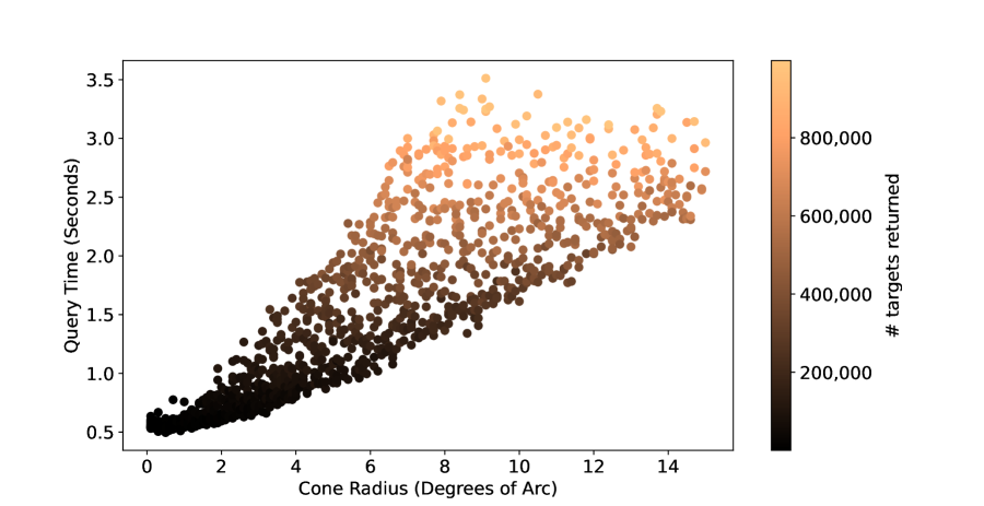
Figure 7.— Cone search lookup speed as a function of radius. Cone centers are sampled at random points across the sky.

The construction of this database presented us with a unique set of problems. Traditional survey data releases have been of static data sets that lend themselves to indexing and partitioning schemes that allow for fast queries. However, Sky Patrol V2.0 is not a static data release. Our light curves are updated in near-real time as we gather new images from our stations. This has forced us to decouple our lookup tables from their corresponding light curves. The lookup tables are kept as in-memory distributed dataframes and the light curves are kept on disk in a document store. Each of these architectures has its own contribution to the speed of our database.

Our in-memory lookup tables do not have pre-calculated indexes on any of their columns. This is a restriction of the software stack we are running. However, this means that we can load new catalogs on-the-fly with little penalty. Also, it means that each one of our queries results in a full table scan. While this would be untenable on disk-based storage, it is trivial for in-memory storage. The major benefit of this is that the speed of our queries is not dictated by the complexity or breadth of their filters, but rather by the number of results they return (i.e., bandwidth limitations). In other words, users can run cone searches with arbitrary radius with little to no penalty.

A major design goal of this architecture was to return all large queries to the lookup table—around 1 million targets—in under a minute, and all small queries—thousands of targets—in under 5 seconds. Figure 3 shows the cone search lookup speeds as a function of radii.

The document store uses our unique internal identifiers as hash keys for each corresponding light curve. This means we can retrieve light curves in $\mathcal{O}(1)$ time, so that retrieval time grows roughly with the number of sources. The speed of these retrievals is only limited by bandwidth. Because the light curve documents contain far more data than their corresponding rows in the lookup tables, retrieval speeds will vary depending on the users bandwidth and latency from our servers at the University of Hawaii. In testing, downloads to Ohio State University ran at a rate of 1,000 light curves per minute per core.

7. Conclusion

ASAS-SN Sky Patrol V2.0 represents a major step forward for survey data releases. While previous tools and data releases have given users the ability to pull live photometry data or run complex searches across a collection of input catalogs, few, if any, have managed to do both at the speed and scale of this project. While Sky Patrol V1.0 still allows users to run small numbers of light curves anywhere on the sky, Sky Patrol V2.0 enables users to perform studies using millions of light curves that are continuously updated.

It is our hope that researchers can leverage our input catalogs and light curves not only in their multi-messenger and time-domain applications, but also in service of standalone science applications. In regards to the latter, this system will serve as the foundation for the ASAS-SN team’s upcoming “Patrol” projects. Each of these patrols will monitor incoming photometry data for certain classes of objects—such as active galactic nuclei, young stellar objects, cataclysmic variables, etc.—in order to detect and study anomalous events in real time. Finally, we are also investigating the possibility of allowing individual users to create custom patrols where the target list and triggering function would be created by community members and run on the ASAS-SN data stream in real time.

References

- Abbott et al. (2020) Abbott B. P., et al., 2020, Phys. Rev. D, 101, 084002
- Abdollahi et al. (2020) Abdollahi S., et al., 2020, The Astrophysical Journal Supplement Series, 247, 33
- Alard (2000) Alard C., 2000, A&AS, 144, 363
- Alard & Lupton (1998) Alard C., Lupton R. H., 1998, ApJ, 503, 325
- Auge et al. (2020) Auge C., et al., 2020, AJ, 160, 18
- Aydi et al. (2019) Aydi E., et al., 2019, arXiv e-prints, p. arXiv:1903.09232
- Aydi et al. (2020a) Aydi E., et al., 2020a, Nature Astronomy,
- Aydi et al. (2020b) Aydi E., et al., 2020b, ApJ, 905, 62
- Bose et al. (2018) Bose S., et al., 2018, ApJ, 853, 57
- Bose et al. (2019) Bose S., et al., 2019, ApJ, 873, L3
- Bredall et al. (2020) Bredall J. W., et al., 2020, MNRAS, 496, 3257
- Brown et al. (2013) Brown T. M., et al., 2013, PASP, 125, 1031
- Brown et al. (2016) Brown J. S., Shappee B. J., Holoien T. W. S., Stanek K. Z., Kochanek C. S., Prieto J. L., 2016, MNRAS, 462, 3993
- Brown et al. (2018) Brown J. S., et al., 2018, MNRAS, 473, 1130
- Brown et al. (2019) Brown J. S., et al., 2019, MNRAS, 484, 3785
- Buchler & Kolláth (2011) Buchler J. R., Kolláth Z., 2011, The Astrophysical Journal, 731, 24
- Campbell et al. (2015) Campbell H. C., et al., 2015, MNRAS, 452, 1060
- Christy et al. (2021) Christy C. T., et al., 2021, Research Notes of the American Astronomical Society, 5, 38
- Christy et al. (2022a) Christy C. T., et al., 2022a, arXiv e-prints, p. arXiv:2205.02239
- Christy et al. (2022b) Christy C. T., et al., 2022b, PASP, 134, 024201
- Dálya et al. (2018) Dálya G., et al., 2018, MNRAS, 479, 2374
- Dong et al. (2016) Dong S., et al., 2016, Science, 351, 257
- Dong et al. (2019) Dong S., et al., 2019, ApJ, 871, 70
- Evans et al. (2010) Evans I. N., et al., 2010, The Astrophysical Journal Supplement Series, 189, 37
- Flesch (2021) Flesch E. W., 2021, VizieR Online Data Catalog, p. VII/290
- Franckowiak et al. (2020) Franckowiak A., et al., 2020, ApJ, 893, 162
- Garrappa et al. (2019) Garrappa S., et al., 2019, ApJ, 880, 103
- Gilbert et al. (2020) Gilbert E. A., et al., 2020, AJ, 160, 116
- Godoy-Rivera et al. (2017) Godoy-Rivera D., et al., 2017, MNRAS, 466, 1428
- Gully-Santiago et al. (2017) Gully-Santiago M. A., et al., 2017, ApJ, 836, 200
- Hanuš et al. (2020) Hanuš J., et al., 2020, A&A, 633, A65
- Herczeg et al. (2016) Herczeg G. J., et al., 2016, ApJ, 831, 133
- Hinkle et al. (2020) Hinkle J. T., Holoien T. W. S., Shappee B. J., Auchettl K., Kochanek C. S., Stanek K. Z., Payne A. V., Thompson T. A., 2020, ApJ, 894, L10
- Hinkle et al. (2021a) Hinkle J. T., et al., 2021a, arXiv e-prints, p. arXiv:2108.03245
- Hinkle et al. (2021b) Hinkle J. T., et al., 2021b, MNRAS, 500, 1673
- Hinkle et al. (2022a) Hinkle J. T., et al., 2022a, arXiv e-prints, p. arXiv:2206.04071
- Hinkle et al. (2022b) Hinkle J. T., et al., 2022b, The Astronomer’s Telegram, 15281, 1
- Holoien et al. (2014a) Holoien T. W.-S., et al., 2014a, MNRAS, 445, 3263
- Holoien et al. (2014b) Holoien T. W.-S., et al., 2014b, ApJ, 785, L35
- Holoien et al. (2016a) Holoien T. W.-S., et al., 2016a, MNRAS, 455, 2918
- Holoien et al. (2016b) Holoien T. W. S., et al., 2016b, MNRAS, 463, 3813
- Holoien et al. (2017a) Holoien T. W.-S., et al., 2017a, MNRAS,
- Holoien et al. (2017b) Holoien T. W.-S., et al., 2017b, MNRAS, 464, 2672
- Holoien et al. (2017c) Holoien T. W. S., et al., 2017c, MNRAS, 464, 2672
- Holoien et al. (2017d) Holoien T. W. S., et al., 2017d, MNRAS, 471, 4966
- Holoien et al. (2018) Holoien T. W. S., Brown J. S., Auchettl K., Kochanek C. S., Prieto J. L., Shappee B. J., Van Saders J., 2018, MNRAS, 480, 5689
- Holoien et al. (2019a) Holoien T. W. S., et al., 2019a, ApJ, 880, 120
- Holoien et al. (2019b) Holoien T. W. S., et al., 2019b, ApJ, 883, 111
- Holoien et al. (2019c) Holoien T. W. S., et al., 2019c, ApJ, 883, 111
- Holoien et al. (2020) Holoien T. W. S., et al., 2020, ApJ, 898, 161
- Holoien et al. (2022) Holoien T. W. S., et al., 2022, ApJ, 933, 196
- IceCube Collaboration et al. (2018) IceCube Collaboration et al., 2018, Science, 361, eaat1378
- Icecube Collaboration et al. (2017) Icecube Collaboration et al., 2017, A&A, 607, A115
- Jacques et al. (2019) Jacques C., Pimentel E., Barros J., 2019, Minor Planet Electronic Circulars, 2019-O56
- Jayasinghe et al. (2018) Jayasinghe T., et al., 2018, MNRAS, 477, 3145
- Jayasinghe et al. (2019a) Jayasinghe T., et al., 2019a, MNRAS, 485, 961
- Jayasinghe et al. (2019b) Jayasinghe T., et al., 2019b, MNRAS, 486, 1907
- Jayasinghe et al. (2019c) Jayasinghe T., et al., 2019c, Monthly Notices of the Royal Astronomical Society, 491, 13
- Jayasinghe et al. (2020a) Jayasinghe T., et al., 2020a, MNRAS, 493, 4045
- Jayasinghe et al. (2020b) Jayasinghe T., et al., 2020b, MNRAS, 493, 4186
- Jayasinghe et al. (2021) Jayasinghe T., et al., 2021, MNRAS,
- Kato et al. (2014a) Kato T., et al., 2014a, PASJ, 66, 30
- Kato et al. (2014b) Kato T., et al., 2014b, PASJ, 66, 90
- Kato et al. (2016) Kato T., et al., 2016, PASJ, 68, 65
- Kato et al. (2017) Kato T., et al., 2017, PASJ, 69, 75
- Kato et al. (2020) Kato T., et al., 2020, PASJ, 72, 14
- Kawash et al. (2021a) Kawash A., et al., 2021a, ApJ, 910, 120
- Kawash et al. (2021b) Kawash A., et al., 2021b, ApJ, 922, 25
- Kawash et al. (2022) Kawash A., et al., 2022, ApJ, 937, 64
- Kochanek et al. (2017a) Kochanek C. S., et al., 2017a, PASP, 129, 104502
- Kochanek et al. (2017b) Kochanek C. S., et al., 2017b, MNRAS, 467, 3347
- Lépine & Gaidos (2011) Lépine S., Gaidos E., 2011, AJ, 142, 138
- Li et al. (2017) Li K.-L., et al., 2017, Nature Astronomy, 1, 697
- Littlefield et al. (2016) Littlefield C., et al., 2016, ApJ, 833, 93
- Mishra et al. (2021) Mishra H. D., et al., 2021, ApJ, 913, 146
- Nasa & Heasarc (2018) Nasa Heasarc 2018, VizieR Online Data Catalog, p. B/swift
- Necker et al. (2022) Necker J., et al., 2022, arXiv e-prints, p. arXiv:2204.00500
- Neumann et al. (2022) Neumann K. D., et al., 2022, arXiv e-prints, p. arXiv:2210.06492
- Neustadt et al. (2020) Neustadt J. M. M., et al., 2020, MNRAS, 494, 2538
- Neustadt et al. (2022) Neustadt J. M. M., et al., 2022, arXiv e-prints, p. arXiv:2211.03801
- O’Grady et al. (2020) O’Grady A. J. G., et al., 2020, ApJ, 901, 135
- Osborn et al. (2017) Osborn H. P., et al., 2017, MNRAS, 471, 740
- Pawlak et al. (2019) Pawlak M., et al., 2019, MNRAS, 487, 5932
- Payne et al. (2021) Payne A. V., et al., 2021, ApJ, 910, 125
- Payne et al. (2022a) Payne A. V., et al., 2022a, arXiv e-prints, p. arXiv:2206.11278
- Payne et al. (2022b) Payne A. V., et al., 2022b, ApJ, 926, 142
- Prentice et al. (2018) Prentice S. J., et al., 2018, ApJ, 865, L3
- Prieto et al. (2017) Prieto J. L., et al., 2017, The Astronomer’s Telegram, 10597, 1
- Rodríguez Martínez et al. (2020) Rodríguez Martínez R., Lopez L. A., Shappee B. J., Schmidt S. J., Jayasinghe T., Kochanek C. S., Auchettl K., Holoien T. W. S., 2020, ApJ, 892, 144
- Rodriguez et al. (2016) Rodriguez J. E., et al., 2016, ApJ, 831, 74
- Rodriguez et al. (2017) Rodriguez J. E., et al., 2017, ApJ, 848, 97
- Rodriguez et al. (2019) Rodriguez J. E., et al., 2019, AJ, 158, 197
- Rowan et al. (2021) Rowan D. M., Stanek K. Z., Jayasinghe T., Kochanek C. S., Thompson T. A., Shappee B. J., Holoien T. W. S., Prieto J. L., 2021, MNRAS, 507, 104
- Rowan et al. (2022a) Rowan D. M., et al., 2022a, arXiv e-prints, p. arXiv:2210.06486
- Rowan et al. (2022b) Rowan D. M., et al., 2022b, MNRAS, 517, 2190
- Schmidt et al. (2014) Schmidt S. J., et al., 2014, ApJ, 781, L24
- Schmidt et al. (2016) Schmidt S. J., et al., 2016, ApJ, 828, L22
- Schmidt et al. (2019) Schmidt S. J., et al., 2019, ApJ, 876, 115
- Secrest et al. (2015) Secrest N. J., Dudik R. P., Dorland B. N., Zacharias N., Makarov V., Fey A., Frouard J., Finch C., 2015, ApJS, 221, 12
- Shappee et al. (2014) Shappee B. J., et al., 2014, ApJ, 788, 48
- Shappee et al. (2016) Shappee B. J., et al., 2016, ApJ, 826, 144
- Shappee et al. (2019a) Shappee B. J., et al., 2019a, ApJ, 870, 13
- Shappee et al. (2019b) Shappee B. J., et al., 2019b, GRB Coordinates Network, 24309, 1
- Shappee et al. (2019c) Shappee B. J., et al., 2019c, GRB Coordinates Network, 24313, 1
- Shappee et al. (2019d) Shappee B. J., et al., 2019d, GRB Coordinates Network, 24323, 1
- Shields et al. (2019) Shields J. V., et al., 2019, MNRAS, 483, 4470
- Sicilia-Aguilar et al. (2017) Sicilia-Aguilar A., et al., 2017, A&A, 607, A127
- Simon et al. (2018) Simon J. D., Shappee B. J., Pojmański G., Montet B. T., Kochanek C. S., van Saders J., Holoien T. W. S., Henden A. A., 2018, ApJ, 853, 77
- Tonry et al. (2018) Tonry J. L., et al., 2018, PASP, 130, 064505
- Trakhtenbrot et al. (2019) Trakhtenbrot B., et al., 2019, ApJ, 883, 94
- Tucker et al. (2018) Tucker M. A., et al., 2018, ApJ, 867, L9
- Tucker et al. (2021) Tucker M. A., et al., 2021, MNRAS, 506, 6014
- Vallely et al. (2019) Vallely P. J., et al., 2019, MNRAS, 487, 2372
- Watson et al. (2006) Watson C. L., Henden A. A., Price A., 2006, Society for Astronomical Sciences Annual Symposium, 25, 47
- Way et al. (2019) Way Z., et al., 2019, The Astronomer’s Telegram, 13346, 1
- Way et al. (2022) Way Z. S., Jayasinghe T., Kochanek C. S., Stanek K. Z., Vallely P., Thompson T. A., Holoien T. W. S., Shappee B. J., 2022, MNRAS, 514, 200
- Wyrzykowski et al. (2020) Wyrzykowski Ł., et al., 2020, A&A, 633, A98
- Yuk et al. (2022) Yuk H., Dai X., Jayasinghe T., Fu H., Mishra H. D., Kochanek C. S., Shappee B. J., Stanek K. Z., 2022, arXiv e-prints, p. arXiv:2203.08348
- Zeldes et al. (2021) Zeldes J., et al., 2021, arXiv e-prints, p. arXiv:2109.04501
- de Jaeger et al. (2022a) de Jaeger T., et al., 2022a, arXiv e-prints, p. arXiv:2210.16329
- de Jaeger et al. (2022b) de Jaeger T., et al., 2022b, MNRAS, 509, 3427
- van Buitenen et al. (2018) van Buitenen G., et al., 2018, Minor Planet Electronic Circulars, 2018-O01