New parametrization of the dark-energy equation of state with a single parameter

Abstract

We propose a novel dark-energy equation-of-state parametrization, with a single parameter $\eta$ that quantifies the deviation from $\Lambda$CDM cosmology. We first confront the scenario with various datasets, from Hubble function (OHD), Supernovae Type Ia (SNIa), baryon acoustic oscillations (BAO), and cosmic microwave background (CMB) observations, and we show that $\eta$ has a preference to a non-zero value, namely a deviation from $\Lambda$CDM cosmology is favoured, although the zero value is marginally inside the 1$\sigma$ confidence level. However, we find that the present Hubble function value acquires a higher value, namely $H_{0}=70.339^{+1.789}_{-1.761}$, which implies that the $H_{0}$ tension can be partially alleviated. Additionally, we perform a cosmographic analysis, showing that the Universe transits from deceleration to acceleration in the recent cosmological past, nevertheless in the future it will not result to a de Sitter phase, since it exhibits a second transition from acceleration to deceleration. Finally, we perform statefinder and Om diagnostic analyses. The scenario behaves similarly to $\Lambda$CDM paradigm at high redshifts, while the deviation becomes significant at late and recent times and especially in the future.

I Introduction

According to acculturating observations the universe in the recent cosmological past entered into a period of accelerating expansion. The first general class of explanations is to introduce new, exotic sectors in the universe content, under the umbrella term dark energy [1, 2] in the framework of general relativity. The second general class is to extend the underlying gravitational theory, in which case the cause of acceleration is of gravitational origin [3, 4, 5, 6, 7].

Nevertheless, at the phenomenological level, both approaches can be quantified through the (effective) dark-energy equation-of-state parameter $w_{x}$. Thus, introducing various parametrizations of $w_{x}$ allows us to describe the universe evolution and confront with observational datasets, to reveal the required dark-energy features in order to obtain agreement. In particular, starting from the simple cosmological constant, a large number of parametrizations have been introduced in the literature, involving one parameter [8, 9], two parameters, such as the Chevallier-Polarski-Linder (CPL) parametrization [10, 11], the Linear parametrization [12, 13, 14], the Logarithmic parametrization [15], the Jassal-Bagla-Padmanabhan parametrization (JBP) [16], the Barboza-Alcaniz (BA) parametrization [17], $H_{0}$ problem at low reshift [18, 19], etc [20, 21, 22, 23, 24, 25, 26, 27, 28, 29, 30, 31, 32, 33, 34, 35, 36, 37, 38, 39, 40, 41, 42, 43, 44, 45, 46, 47]. Additionally, note that one can impose the parametrization at the deceleration parameter level [48, 49, 50], at equation-of-sate (EoS) parameter level [51] or even at the Hubble parameter level [52, 53, 55, 54].

In the present manuscript we propose a novel dark-energy equation-of-state parametrization, with a single parameter $\eta$ that quantifies the deviation from $\Lambda$CDM cosmology. Additionally, under this scenario, dark energy behaves like cosmological constant at high redshifts, while the deviation becomes significant at low and recent redshifts, and especially in the future. Finally, for $\eta=0$ we recover $\Lambda$CDM cosmology completely. As we will see, apart form being capable of fitting the data, the new parametrization can partially alleviate the $H_{0}$ tension too, since it leads to a $H_{0}$ value in between the Planck one and the one from direct measurements [56, 57].

The article is organized as follows. In Section II we present the novel dark-energy parametrization. Then in Section III we perform a detailed confrontation with observations, namely with Hubble function (OHD), Supernovae Type Ia (SNIa), baryon acoustic oscillations (BAO), and cosmic microwave background (CMB) data. In Section IV we perform a cosmographic analysis and we apply the Statefinder and Om diagnostics. Finally, Section V is devoted to the conclusions. Lastly, the details of the various datasets and the corresponding fitting procedure is given in the Apendix.

II New single-parameter equation-of-state parametrization

In this section we first briefly review the basic equations of any cosmological scenario, and then we introduce the new parametrization for the dark-energy equation of state, with just a single parameter. We consider the usual homogeneous and isotropic Friedmann-Robertson-Walker (FRW) metric

$${\rm d}s^{2}=-{\rm d}t^{2}+a^{2}(t)\left[\frac{{\rm d}r^{2}}{1-Kr^{2}}+r^{2}\left(d\theta^{2}+\sin^{2}\theta d\phi^{2}\right)\right],$$ (1)

with $a(t)$ the scale factor and $K$ the spatial-curvature parameter, ($K=0,-1,+1$ for spatially flat, open and closed universe, respectively). Furthermore, we consider that the universe is filled with baryonic and dark matter, radiation as well as the effective dark-energy fluid. Hence, the Friedmann equations that determine the background evolution of the Universe are

$$H^{2}+\frac{K}{a^{2}} = \frac{8\pi G}{3}\rho_{tot},$$ (2)

$$2\dot{H}+3H^{2}+\frac{K}{a^{2}} = -8\pi G\,p_{tot},$$ (3)

where $G$ is the gravitational constant and $H=\dot{a}/a$ the Hubble function, with dots marking time derivatives. The total energy density and pressure are thus given as $\rho_{tot}=\rho_{r}+\rho_{b}+\rho_{c}+\rho_{x}$ and $p_{tot}=p_{r}+p_{b}+p_{c}+p_{x}$, where the subscripts $r,\;b,\;c,\;x$ stand respectively for radiation, baryon, cold dark matter and dark energy. As usual, and without loss of generality, we focus on the spatially flat case and therefore in the following we impose $K=0$. Finally, assuming that the various sectors do not interact mutually we deduce that they are separately conserved, following the conservation equations

$$\dot{\rho}_{i}+3H(1+w_{i})\rho_{i}=0,$$ (4)

where $i\in\{r,b,c,x\}$. In the above expression we have introduced the equation-of-state parameter of each fluid as $p_{i}\equiv w_{i}\rho_{i}$.

We proceed by providing for completeness the evolution equations of the Universe at the perturbation level. In synchronous gauge, the perturbed metric reads as

$$ds^{2}=a^{2}(\eta)\left[-d\eta^{2}+(\delta_{ij}+h_{ij})dx^{i}dx^{j}\right],$$ (5)

with $\eta$ the conformal time, and where $\delta_{ij}$ and $h_{ij}$ denote the unperturbed and the perturbed metric parts (with $h=h^{j}_{j}$ the trace). Perturbing additionally the universe fluids and transforming to the Fourier space we finally extract [58, 59, 60]:

$$\delta^{\prime}_{i}=-(1+w_{i})\,\left(\theta_{i}+\frac{h^{\prime}}{2}\right)-3\mathcal{H}\left(\frac{\delta p_{i}}{\delta\rho_{i}}-w_{i}\right)\delta_{i}-9\mathcal{H}^{2}\left(\frac{\delta p_{i}}{\delta\rho_{i}}-c^{2}_{a,i}\right)(1+w_{i})\frac{\theta_{i}}{{k}^{2}},$$ (6)

$$\theta^{\prime}_{i}=-\mathcal{H}\left(1-3\frac{\delta p_{i}}{\delta\rho_{i}}\right)\theta_{i}+\frac{\delta p_{i}/\delta\rho_{i}}{1+w_{i}}\,{k}^{2}\,\delta_{i}-{k}^{2}\sigma_{i},$$ (7)

with primes denoting conformal-time derivative and with $\mathcal{H}=a^{\prime}/a$ the conformal Hubble function, and where ${k}$ is the mode wavenumber. Moreover, $\delta_{i}=\delta\rho_{i}/\rho_{i}$ stands for the overdensity of the $i$-th fluid, $\theta_{i}\equiv ik^{j}v_{j}$ marks the divergence of the $i$-th fluid velocity, and $\sigma_{i}$ is the corresponding anisotropic stress. Lastly, $c_{a,i}^{2}=\dot{p}_{i}/\dot{\rho}_{i}$ is the adiabatic sound speed given as $c^{2}_{a,i}=w_{i}-\frac{w_{i}^{\prime}}{3\mathcal{H}(1+w_{i})}$.

Let us now introduce the new dark-energy parametrization. As usual, knowing the equation of state of a fluid allows as to extract its time-evolution by solving the conservation equation (4). For radiation, we have $w_{r}=1/3$ and thus we obtain $\rho_{r}=\rho_{r_{0}}\,a^{-4}$ (setting the scale factor at present to 1), while for baryonic and dark matter we have $w_{b}=w_{c}=0$, which leads to $\rho_{b}=\rho_{b_{0}}\,a^{-3}$ and $\rho_{c}=\rho_{c_{0}}\,a^{-3}$, where $\rho_{i_{0}}$ stands for the present density value of the $i$-th fluid. Concerning for the equation-of-state parameter of the dark-energy sector, since it is unknown, as we mentioned in the Introduction one can consider various parametrizations. Focusing on the barotropic fluid sub-class we consider that it is a function of time only, or equivalently of the scale factor $a$, i.e. $w_{x}(a)$. Hence, the solution of the dark-energy conservation equation leads to

$$\rho_{x}(a)=\rho_{x_{0}}\,a^{-3}\exp\left[-3\int_{1}^{a}\frac{w_{x}\left(a^{\prime}\right)}{a^{\prime}}\,da^{\prime}\right].$$ (8)

In this work we consider that the energy density of the dark-energy sector evolves as

$$\rho_{x}(a)=ce^{-\eta a}\tan(a^{\eta}),$$ (9)

where $\eta$ is the single parameter, and $c=\rho_{x_{0}}\frac{e^{\eta}}{\tan{1}}$. Inserting this into (8) we easily extract the dark-energy equation-of-state parameter as

$$w_{x}(a)=-1+\frac{\eta a}{3}+\frac{\frac{\eta}{a^{\eta}}}{\sqrt{\left(1+\frac{1}{a^{2\eta}}\right)}\,\arctan\big{(}\frac{1}{a}\big{)}^{\eta}}.$$ (10)

Hence, introducing for convenience the redshift $z$ as the independent variable (where $a^{-1}=1+z$) the above relation becomes

$$w_{x}(z)=-1+\frac{\eta}{3(1+z)}+\frac{\eta(1+z)^{\eta}}{\sqrt{\left[1+(1+z)^{2\eta}\right]}\,\arctan(1+z)^{\eta}}.$$ (11)

Relation (11) is the novel parametrization of the dark-energy equation-of-state parameter that we propose in this work. In the case $\eta=0$ we recover $\Lambda$CDM concordance model, where $w_{x}=-1$ and $\rho_{x}=\rho_{x_{0}}=const$. However, in the general case the parameter $\eta$ quantifies the deviation form $\Lambda$CDM scenario.

Inserting the above parametrization in the first Friedmann equation (2) we obtain

$$H=H_{0}\sqrt{\left[(\Omega_{b_{0}}+\Omega_{c_{0}})(1+z)^{3}+\Omega_{r_{0}}(1+z)^{4}+\Omega_{x_{0}}e^{\frac{\eta z}{1+z}}\frac{\arctan(1+z)^{\eta}}{\arctan 1}\right]},$$ (12)

with $H_{0}$ the present value of the Hubble parameter, and where we have introduced the present values of the density parameters $\Omega_{i_{0}}\equiv\frac{8\pi G}{3H^{2}}\rho_{i_{0}}$ (hence the present value of the total matter density parameter is ${\Omega_{m_{0}}}\equiv{\Omega_{b_{0}}}+{\Omega_{c_{0}}}$). This expression allows us to investigate the cosmological evolution in detail, and confront it with observational datasets.

Lastly, from parametrization (11) and the corresponding Hubble function (12), we can straightforwardly calculate various quantities. In particular, the deceleration parameter $q=-1-\dot{H}{H^{-2}}$ is given by

$$q(z)=-1+\frac{\Big{[}3(1+z)^{4}\Omega_{m_{0}}+\frac{4\eta\Omega_{x_{0}}(1+z)^{2}e^{\frac{\eta z}{1+z}}\arctan(1+z)^{\eta-1}}{\pi(z^{2}+2z+2)}+\frac{4\eta\Omega_{x_{0}}e^{\frac{\eta z}{1+z}}\arctan(1+z)^{\eta}}{\pi}\Big{]}}{2(1+z)\Big{[}(1+z)^{3}\Omega_{m_{0}}+\frac{4\Omega_{x_{0}}e^{\frac{\eta z}{1+z}}\arctan(1+z)^{\eta}}{\pi}\Big{]}},$$ (13)

while the higher-order cosmographic parameters [61] read as

$$j=-q+2q(1+q)+(1+z)\frac{dq}{dz},$$ (14)

$$s=j-3j(1+q)-(1+z)\frac{dj}{dz},$$ (15)

$$l=s-4s(1+q)-(1+z)\frac{ds}{dz},$$ (16)

$$m=l-5l(1+q)-(1+z)\frac{dl}{dz}.$$ (17)

Similarly, for the matter and dark-energy density parameters we obtain

$$\Omega_{m}(z)=\frac{1}{1+\frac{4\Omega_{x_{0}}e^{\frac{\eta z}{1+z}}\arctan(1+z)^{\eta}}{\pi\Omega_{b_{0}}(1+z)^{3}}},$$ (18)

and

$$\Omega_{x}(z)=\frac{1}{1+\frac{\pi\,\Omega_{b_{0}}e^{\frac{-\eta z}{1+z}}[(1+z)^{3}\arctan(1+z)^{-\eta}]}{4\,\Omega_{x_{0}}}}.$$ (19)

III Observational constraints

In the previous section we proposed a new parametrization for the dark-energy equation of state, given by (11), which has a single parameter, namely $\eta$. In this section, we perform a detailed confrontation with various datasets, focusing on the bounds of $\eta$. In particular, we will use data from: (i) Hubble function observations (OHD) with 77 data points [62], (ii) Supernovae Type Ia (SNIa) observations from Union 2.1 compilation dataset [63] (iii) baryon acoustic oscillations (BAO), and (iv) cosmic microwave background (CMB). The details of the datasets and the corresponding methodology, are given in the Appendix.

Let us not present the constraints we obtain after applying the above formalism and datasets in the Friedmann equations at hand, focusing on the new model parameter $\eta$. In Fig. 1 we present the likelihood contours in the $\eta$-$H_{0}$ plane with $1\sigma$, $2\sigma$ and $3\sigma$ confidence levels, around the best-fit values. Additionally, in Table 1 we summarize the obtained results, and we provide the corresponding $\chi^{2}$. Finally, in Table 2 we summarize other cosmological parameters, such as the density parameters and the deceleration parameter, the equation-of-state parameters, and the transition redshift.

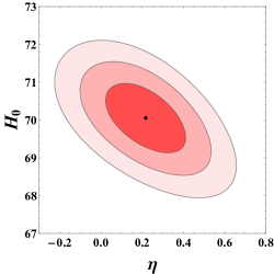
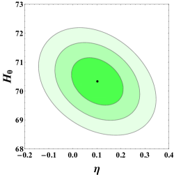
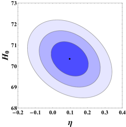
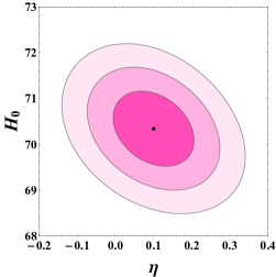
Figure 1: The likelihood contours in the $\eta$-$H_{0}$ plane, with $1\sigma$, $2\sigma$ and $3\sigma$ confidence levels, for $H(z)$ data (upper left), $H(z)+SNIa$ data (upper right), for $H(z)+SNIa+BAO$ data (lower left), and for the joint analysis of $H(z)+SNIa+BAO+BAO/CMB$ data (lower right). The black dots represent the best-fit values.

Table 1: Summary of the observational constraints on the model parameter $\eta$ and on the current Hubble function $H_{0}$, from various datasets, alongside the corresponding $\chi^{2}_{min}$.

Dataset	$\chi^{2}_{min}$	$H_{0}$ (km/s/Mpc)	$\eta$
$H(z)$ (77 points data)	$52.436$	$70.057^{+1.777}_{-1.753}$	$0.217^{+0.387}_{-0.359}$
$\!\!H(z)$ + $SNIa$	$615.852$	$70.334^{+1.784}_{-1.766}$	$0.102^{+0.233}_{-0.230}$
$H(z)$ + $SNIa$+ $BAO$	$631.801$	$70.345^{+1.775}_{-1.775}$	$0.098^{+0.236}_{-0.230}$
$H(z)$ + $SNIa$ + $BAO/CMB$	$620.722$	$70.329^{+1.769}_{-1.771}$	$0.105^{+0.233}_{-0.229}$
$H(z)$ + $SNIa$ + $BAO$ + $BAO/CMB$	$636.675$	$70.339^{+1.789}_{-1.761}$	$0.100^{+0.231}_{-0.228}$

Table 2: Summary of the constraints on the deceleration parameter $q$, the transition redshift $z_{tr}$, the current value of the dark-energy equation-of-state parameter $w_{x_{0}}$, the total matter density parameter at present ${\Omega_{m_{0}}}\equiv{\Omega_{b_{0}}}+{\Omega_{c_{0}}}$, and the dark-energy density parameter at present ${\Omega_{x_{0}}}$.

Dataset	$q$	$z_{tr}$	${w_{x_{0}}}$	$\ \ \ \ \ \ \ \ {\Omega_{m_{0}}}\ \ \ \ \ \ \ \$	${\Omega_{x_{0}}}$
$H(z)$ (77 points data)	$-0.513^{+0.105}_{-0.112}$	$\ \ \ \simeq 0.927\ \ \$	$-0.732^{+0.200}_{-0.208}$	$0.2757^{+0.0079}_{-0.0081}$	$0.7243^{+0.0081}_{-0.0079}$
$\ H(z)$ + $SNIa$	$-0.591^{+0.067}_{-0.072}$	$\ \ \ \simeq 0.927\ \ \$	$-0.874^{+0.125}_{-0.133}$	$0.2702^{+0.0048}_{-0.0051}$	$0.7298^{+0.0051}_{-0.0048}$
$\ \,H(z)$ + $SNIa$ + $BAO$	$-0.595^{+0.067}_{-0.069}$	$\ \ \ \simeq 0.927\ \ \$	$-0.879^{+0.125}_{-0.126}$	$0.2670^{+0.0049}_{-0.0049}$	$0.7300^{+0.0049}_{-0.0049}$
$H(z)$ + $SNIa$ + $BAO/CMB$	$-0.590^{+0.066}_{-0.068}$	$\ \ \ \simeq 0.927\ \ \$	$-0.871^{+0.123}_{-0.126}$	$0.2703^{+0.0048}_{-0.0049}$	$0.7297^{+0.0049}_{-0.0048}$
$H(z)$ + $SNIa$ + $BAO$ + $BAO/CMB$	$-0.593^{+0.066}_{-0.069}$	$\ \ \ \simeq 0.927\ \ \$	$-0.876^{+0.124}_{-0.126}$	$0.2701^{+0.0048}_{-0.0048}$	$0.7299^{+0.0048}_{-0.0048}$

As we observe, the new model parameter $\eta$ that quantifies the deviation from $\Lambda$CDM cosmology has a preference to a non-zero value, although zero is marginally inside the 1$\sigma$ confidence level. Concerning $H_{0}$ we observe that we obtain a higher value comparing to $\Lambda$CDM scenario, although a bit lower than the direct measurements [56], which implies that the new dark-energy parametrization at hand can partially alleviate the $H_{0}$ tension. This is an additional result of the present work.

IV Cosmographic analysis and Statefinder diagnostic

In this section, for completeness, we perform the cosmographic analysis of the cosmological scenario with the new dark-energy parametrization, and we apply the Statefinder diagnostic. For simplicity we neglect the radiation sector.

Let us start with the deceleration parameter given in (13). Using the best-fit values of the model parameters given in Tables 1-2, we plot $q(z)$ in Fig. 2. As we can see, we obtain the transition from deceleration to acceleration at the transition redshift $z_{tr}$ in agreement with observations. However, it is interesting to note that the novel parametrization at hand will lead to a second transition in the future, at redshift $z_{tr_{2}}$, from acceleration to deceleration (at around $z_{tr_{2}}\approx-0.9$).

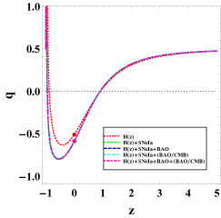
Figure 2: The evolution of the deceleration parameter $q$ in terms of the redshift $z$, using the best-fit values of the model parameters given in Tables 1-2. The red dots mark the present values.

We proceed to the examination of the other cosmographic parameters given in (14)-(17). In particular, we use the best-fit values of the model parameters given in Tables 1-2, and in Fig. 3 we present their evolution. Additionally, in Table 3 we summarize their values at present. Since in $\Lambda$CDM paradigm the value of the jerk parameter is equal to unity ($j=1$), the deviation from $j=1$ quantifies the deviation of a dark-energy scenario from the concordance model. Again we find that the new proposed dark-energy parametrization behaves similarly to $\Lambda$CDM scenario at high redshifts, while the deviation becomes more significant at late and recent times, and especially in the future. Finally, the same features can be obtained from the evolution of the snap $s$, lerk $l$ and $m$ parameters.

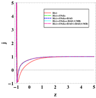
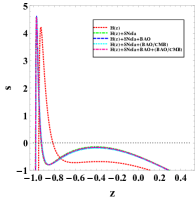
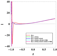
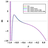
Figure 3: The evolution of the cosmographic parameters $j,s,l,m$ given in (14)-(17), in terms of the redshift $z$, using the best-fit values of the model parameters given in Tables 1-2.

Table 3: Summary of the constraints on the present values of the cosmographic parameters, namely jerk $j$, snap $s$, lerk $l$ and $m$ parameters, as well as on the present values of the statefinder diagnostic parameters $r$ and $s^{*}$.

Dataset	$j$	$s$	$l$	$m$	$r$	$s^{*}$
$H(z)$ (77 points data)	$0.524^{+0.341}_{-0.269}$	$-0.878^{+0.563}_{-0.210}$	$1.831^{+0.086}_{-0.686}$	$-8.417^{+1.368}_{-1.150}$	$0.549^{+0.341}_{-0.269}$	$0.148^{+0.124}_{-0.123}$
$\ \ H(z)$ + $SNIa$	$0.762^{+0.238}_{-0.200}$	$-0.509^{+0.489}_{-0.309}$	$1.811^{+0.483}_{-0.041}$	$-7.919^{+1.703}_{-0.653}$	$0.775^{+0.238}_{-0.200}$	$0.069^{+0.074}_{-0.076}$
$H(z)$ + $SNIa$ + $BAO$	$0.772^{+0.227}_{-0.201}$	$-0.491^{+0.468}_{-0.315}$	$1.823^{+0.470}_{-0.024}$	$-7.882^{+1.644}_{-0.674}$	$0.784^{+0.227}_{-0.201}$	$0.066^{+0.074}_{-0.073}$
$H(z)$ + $SNIa$ + $BAO/CMB$	$0.770^{+0.225}_{-0.198}$	$-0.518^{+0.457}_{-0.303}$	$1.806^{+0.431}_{-0.048}$	$-7.937^{+1.544}_{-0.639}$	$0.770^{+0.225}_{-0.198}$	$0.070^{+0.073}_{-0.074}$
$H(z)$ + $SNIa$ $BAO$ + $BAO/CMB$	$0.767^{+0.226}_{-0.199}$	$-0.501^{+0.462}_{-0.310}$	$1.816^{+0.454}_{-0.032}$	$-7.902^{+1.600}_{-0.659}$	$0.779^{+0.225}_{-0.199}$	$0.067^{+0.073}_{-0.073}$

Let us now come to the statefinder diagnostic, which is based on higher derivatives of the scale factor [64, 65, 66]. In particular, one introduces a pair of geometrical parameters $\{r,s^{*}\}$ in order to examine the dynamics of different dark-energy models [67, 68]. The pair of parameters $\{r,s^{*}\}$ are defined as:

$$r=\frac{\dddot{a}}{aH^{3}}\text{, \ \ }s^{*}=\frac{r-1}{3(q-\frac{1}{2})},$$ (20)

with $q\neq\frac{1}{2}$. For our parametrization (8), the expression for $r$ is found to be

$$r=\frac{r_{1}+r_{2}+r_{3}}{(1+z)^{2}[2+z(2+z)]^{2}\tan^{-1}(1+z)^{2}\left[\pi(1+z)^{3}\Omega_{b_{0}}+4e^{\frac{\eta z}{1+z}}\Omega_{x_{0}}\tan^{-1}(1+z)^{\eta}\right]},$$ (21)

where

$$r_{1}=\pi(1+z)^{5}[2+z(2+z)]^{2}\Omega_{m_{0}}\tan^{-1}(1+z)^{2}+2e^{\frac{\eta z}{1+z}}(1+z)^{4}(\eta-1)\eta\Omega_{x_{0}}\tan^{-1}(1+z)^{\eta},$$

$$r_{2}=4e^{\frac{\eta z}{1+z}}\eta\left\{2\eta-3+z[2\eta-7+z(\eta-2z-6)]\right\}\Omega_{x_{0}}\tan^{-1}(1+z)^{1+\eta},$$

$$r_{3}=2e^{\frac{\eta z}{1+z}}[2+z(2+z)]^{2}[2(1+z)^{2}-4(1+z)\eta+\eta^{2}]\Omega_{x_{0}}\tan^{-1}(1+z)^{2+\eta}.$$ (22)

Finally, the expression for $s^{*}$ is obtained using (13) and (21).

In Fig. 4 we present trajectories for different observational datasets in the $q-r$ plane. As we can see, all trajectories start from the decelerating zone, enter into the accelerating zone behaving close to $\Lambda$CDM at present time, and in the far future they converge to the CDM model without cosmological constant (namely $SCDM$ model) without resulting to the de Sitter ($dS$) phase. The present values of parameters $\{r,s^{*}\}$ of statefinder diagnostic are also given in Table 3.

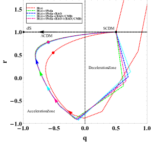
Figure 4: Statefinder diagnostic trajectories in the $q-r$ plane, using the best-fit values of the model parameters given in Tables 1-2. The red dots mark the present values.

Finally, we close this section with the examination of the diagnostic tool known as Om diagnostic [69, 70], which is employed to distinguish among dark-energy models by analyzing the behaviour of different trajectories of $Om(z)$, given as

$$Om(z)=\frac{-1+\left[\frac{H(z)}{H_{0}}\right]^{2}}{-1+(1+z)^{3}},$$ (23)

which in our case, using the Hubble evolution (12) becomes

$$Om(z)=\frac{-1+(1+z)^{3}\Omega_{m_{0}}+\frac{4\,e^{\frac{z\eta}{1+z}}\Omega_{x_{0}}\tan^{-1}(1+z)^{\eta}}{\pi}}{-1+(1+z)^{3}}.$$ (24)

As we can see, the new parametrization at hand at high redshifts behave as $\Lambda$CDM, while the deviation appears at small-redshifts and present time.

V Conclusions

In this work we proposed a novel dark-energy equation-of-state parametrization, with a single parameter $\eta$ that quantifies the deviation from $\Lambda$CDM cosmology. Firstly, we confronted the scenario with various datasets, from Hubble function (OHD), Supernovae Type Ia (SNIa), baryon acoustic oscillations (BAO), and cosmic microwave background (CMB) observations, and we presented the corresponding likelihood contours. As we saw, the new model parameter $\eta$ has a preference to a non-zero value, namely a deviation from $\Lambda$CDM cosmology is favoured, although the zero value is marginally inside the 1$\sigma$ confidence level. However, interestingly enough, we find that $H_{0}$ acquires a higher value comparing to $\Lambda$CDM scenario, which implies that the new dark-energy parametrization at hand can partially alleviate the $H_{0}$ tension.

Additionally, we performed a cosmographic analysis, examining the cosmographic parameters, namely deceleration $q$, jerk $j$, snap $s$, lerk $l$ and $m$ parameters. As we showed, in the scenario at hand the Universe transits from deceleration to acceleration in the recent cosmological past, however in the future it will not result to a de Sitter phase, since a second transition (at $z_{tr_{2}}\approx-0.9$) will lead from acceleration to deceleration. Additionally, we found that the scenario behaves similarly to $\Lambda$CDM paradigm at high redshifts, while the deviation becomes significant at late and recent times (and thus the $H_{0}$ tension is alleviated), and especially in the future.

Finally, we performed a statefinder diagnostic analysis, as well as we applied the Om diagnostic. As we saw, all trajectories start from the decelerating zone, enter into the accelerating zone behaving close to $\Lambda$CDM at present time, while in the far future they converge to deceleration without resulting to the de Sitter phase.

In summary, the new parametrization of the dark-energy equation of state with a single parameter is efficient in describing the data, as well as it can alleviate the $H_{0}$ tension. Hence, it would be worthy to proceed to more detail investigations, such as to examine it at the perturbation level, and in particular relating to the $\sigma_{8}$ tension. Such an analysis will be performed in a separate project.

Acknowledgements

J. K. Singh wishes to thank M. Sami and S. G. Ghosh, for fruitful discussions.

Appendix A Observational data

In this Appendix we present the observational datasets we use in our analysis, and we provide the relevant methodology and the corresponding $\chi^{2}$.

A.1 $H(z)$ data

In the case of observational Hubble data (OHD) the corresponding $\chi^{2}$ of the maximum likelihood analysis is given by

$$\chi_{OHD}^{2}(\eta,H_{0})=\sum\limits_{i=1}^{29}\left[\frac{H_{th}(\eta,H_{0},z_{i})-H_{obs}(z_{i})}{\sigma_{H(z_{i})}}\right]^{2},$$ (25)

where $H(z_{i})$ is evaluated at redshift $z_{i}$, while $H_{th}$ and $H_{obs}$ represent the theoretical and observed value, and $\sigma_{H(z_{i})}$ is the standard deviation. The detailed $H(z)$ data, namely the 77 points, are given in Table 4 below.

Table 4: The 77 Hubble Parameter Data from $H(z)$ measurements used in the present analysis in units of $\mathrm{km\,s^{-1}Mpc^{-1}}$. Method (a) corresponds to Cosmic chronometric method, method (b) to $BAO$ signal in galaxy distribution, and method (c) to $BAO$ signal in $Ly\alpha$ forest distribution alone, or cross-correlated with $QSOs$.

$z$	$H(z)$ $(km/s/Mpc)$	Method	Reference
0.00	69.1$\pm$ 1.3	a	[71]
0.07	70.4$\pm$ 20	a	[72]
0.07	69.0$\pm$ 19.6	a	[72]
0.09	70.4$\pm$ 12.2	a	[73]
0.10	70.4$\pm$ 12.2	a	[72]
0.120	68.6$\pm$ 26.2	a	[72]
0.12	70.0$\pm$ 26.7	a	[71]
0.170	83.0$\pm$ 8	a	[73]
0.170	84.7$\pm$ 8.2	a	[73]
0.179	76.5$\pm$ 4	a	[74]
0.1791	75.0$\pm$ 4	a	[74]
0.199	76.5$\pm$ 5.1	a	[74]
0.1993	75.0$\pm$ 5	a	[74]
0.200	72.9$\pm$ 29.6	a	[72]
0.20	74.4$\pm$ 30.2	a	[72]
0.24	81.5$\pm$ 2.7	b	[75]
0.27	78.6$\pm$ 14.3	a	[73]
0.280	88.8$\pm$ 36.3	a	[72]
0.28	90.6$\pm$ 37.3	a	[71]
0.35	84.4$\pm$ 8.6	b	[71]
0.3519	83.0$\pm$ 14	a	[74]
0.352	84.7$\pm$ 14.3	a	[74]
0.38	81.5$\pm$ 1.9	b	[76]
0.3802	83.0$\pm$ 13.5	a	[77]
0.3802	84.7$\pm$ 14.1	a	[77]
0.40	95.0$\pm$ 17	a	[73]
0.40	96.9$\pm$ 17.3	a	[73]
0.4004	77.0$\pm$ 10.2	a	[77]
0.4004	78.6$\pm$ 10.4	a	[77]
0.4247	87.1$\pm$ 11.2	a	[77]
0.4247	88.9$\pm$ 11.4	a	[77]
0.43	88.3$\pm$ 3.8	a	[71]
0.44	84.3$\pm$ 7.9	a	[78]
0.4497	92.8$\pm$ 12.9	a	[77]
0.4497	94.7$\pm$ 13.1	a	[77]
0.470	89.0$\pm$ 34.0	a	[79]
0.47	90.8$\pm$ 50.6	a	[79]
0.4783	80.0$\pm$ 99.0	a	[77]
0.4783	82.5$\pm$ 9.2	a	[77]
0.48	99.0$\pm$ 63.2	a	[79]
0.51	90.8$\pm$ 1.9	b	[76]
0.57	98.8$\pm$ 3.4	b	[72]
0.593	104.0$\pm$ 13.0	a	[74]
0.593	106.1$\pm$ 13.3	a	[74]
0.60	89.7$\pm$ 6.2	a	[72]
0.61	97.8$\pm$ 2.1	b	[76]
0.64	98.82$\pm$ 2.98	b	[80]

$z$	$H(z)$ $(km/s/Mpc)$	Method	Reference
0.6797	92.0$\pm$ 8	a	[74]
0.68	93.9$\pm$ 8.1	a	[74]
0.73	99.3$\pm$ 7.1	a	[78]
0.7812	105.0$\pm$ 12	a	[74]
0.781	107.1$\pm$ 12.2	a	[74]
0.875	127.6$\pm$ 17.3	a	[74]
0.8754	125.0$\pm$ 17	a	[74]
0.88	91.8$\pm$40.8	a	[81]
0.880	90.0$\pm$ 40	a	[79]
0.90	69.0 $\pm$ 12	a	[73]
0.90	119.4$\pm$ 23.4	a	[73]
0.900	117.0$\pm$ 23	a	[73]
1.037	157.2$\pm$ 20.4	a	[74]
1.037	154.0$\pm$ 20	a	[74]
1.30	171.4$\pm$ 17.3	a	[73]
1.300	168.0$\pm$ 17	a	[73]
1.363	160.0$\pm$ 33.6	a	[82]
1.363	163.3$\pm$ 34.3	a	[82]
1.430	177.0$\pm$ 18	a	[73]
1.43	180.6$\pm$ 18.3	a	[73]
1.530	140.0$\pm$ 14	a	[73]
1.53	142.9$\pm$ 14.2	a	[73]
1.750	202.0$\pm$ 40	a	[73]
1.75	206.1$\pm$ 40.8	a	[73]
1.965	186.5$\pm$ 50.4	a	[82]
1.965	190.3$\pm$ 51.4	a	[82]
2.30	228.0$\pm$ 8.1	c	[83]
2.34	226.5$\pm$ 7.1	c	[83]
2.36	230.6$\pm$ 8.2	c	[84]

A.2 Supernova Type Ia (SNIa) data

We use the latest Union $2.1$ compilation dataset. In this case, we have

$$\chi_{SNIa}^{2}(\eta,H_{0})=\sum\limits_{i=1}^{580}\left[\frac{\mu_{th}(\eta,H_{0},z_{i})-\mu_{obs}(z_{i})}{\sigma_{\mu(z_{i})}}\right]^{2},$$ (26)

where $\mu_{th}$ and $\mu_{obs}$ are the theoretical and observed distance modulus, and $\sigma_{\mu(z_{i})}$ the standard deviation. The distance modulus $\mu(z)$ is defined as

$$\mu(z)=m-M=5LogD_{l}(z)+\mu_{0},$$ (27)

where $m$ and $M$ denote the apparent and absolute magnitudes. Additionally, the luminosity distance $D_{l}(z)$ for flat Universe and the nuisance parameter $\mu_{0}$ are given by

$$D_{l}(z)=(1+z)H_{0}\int_{0}^{z}\frac{1}{H(z^{*})}dz^{*},$$ (28)

and

$$\mu_{0}=5Log\Big{(}\frac{H_{0}^{-1}}{1Mpc}\Big{)}+25,$$ (29)

respectively.

A.3 Baryon acoustic oscillations (BAO)

Concerning Baryon Acoustic Oscillations (BAO) we use the data from Sloan Digital Sky Survey ($SDSS$) [85], $6dF$ Galaxy survey ($6dFGS$) [86], $BOSS\,CMASS$ [87] and three parallel measurements from $WiggleZ$ survey [88]. In BAO observations the distance redshift ratio $d_{z}$ is

$$d_{z}=\frac{r_{s}(z^{*})}{D_{v}(z)},$$ (30)

where $z^{*}=1090$ is the redshift at the time of photon decoupling [89], and $r_{s}(z^{*})$ is the corresponding comoving sound horizon [90]. The dilation scale defined by Eisenstein et al. [91] is

$$D_{v}(z)=\left[(1+z)^{2}\frac{d^{2}_{A}(z)z}{H(z)}\right]^{\frac{1}{3}},$$ (31)

where $d_{A}(z)$ is the angular diameter distance, which essentially is a geometric mean of two transverse and one radial direction. The value of $\chi_{BAO}^{2}$ is given by [92]

$$\chi_{BAO}^{2}=A^{T}C^{-1}A,$$ (32)

where

$$A=\left[{\begin{array}[]{cc}\frac{d_{A}(z^{*})}{D_{v}(0.106)}-30.84\\ \frac{d_{A}(z^{*})}{D_{v}(0.35)}-10.33\\ \frac{d_{A}(z^{*})}{D_{v}(0.57)}-6.72\\ \frac{d_{A}(z^{*})}{D_{v}(0.44)}-8.41\\ \frac{d_{A}(z^{*})}{D_{v}(0.6)}-6.66\\ \frac{d_{A}(z^{*})}{D_{v}(0.73)}-5.43\\ \end{array}}\right],$$

and the inverse covariance matrix $C^{-1}$ is

$$C^{-1}=\left[{\begin{array}[]{cccccc}0.52552&-0.03548&-0.07733&-0.00167&-0.00532&-0.00590\\ -0.03548&24.97066&-1.25461&-0.02704&-0.08633&-0.09579\\ -0.07733&-1.25461&82.92948&-0.05895&-0.18819&-0.20881\\ -0.00167&-0.02704&-0.05895&2.91150&-2.98873&1.43206\\ -0.00532&-0.08633&-0.18819&-2.98873&15.96834&-7.70636\\ -0.00590&-0.09579&-0.20881&1.43206&-7.70636&15.28135\\ \end{array}}\right],$$

approaching the correlation coefficients available in [93, 92, 53].

A.4 Baryon acoustic oscillations and Cosmic microwave background

We use the combined $BAO/CMB$ constraints which were derived by Giostri et al. [92], and we define the comoving sound horizon at the decoupling as

$$r_{s}(z^{*})=\frac{c}{\sqrt{3}}\int_{0}^{(1+z^{*})^{-1}}\frac{1}{a^{2}H(a)\sqrt{1+3(\Omega_{b0}/\Omega_{\gamma 0})a}}da,$$ (33)

where $\Omega_{b0}$ and $\Omega_{\gamma 0}$ are the density parameters of baryon and photon at present, while $z_{d}\approx 1020$ is the redshift at the drag epoch. Rather than including priors on ${\Omega_{b}}h^{2}$ to break the degeneracy between ${\Omega_{b}}h^{2}$ and the distance constraint, we can fit the ratio $\frac{r_{s}(z_{d})}{D_{V}(z_{eff})}$, where $r_{s}(z_{d})$ is the sound horizon at the baryon drag epoch $z_{d}$. In principle, it will be less efficient if the fit is driven by the shape of the correlation function. During the fit we calculate $r_{s}(z_{d})$ using the fitting formula of [94]. Finally, we define the acoustic scale $l_{A}$ as

$$l_{A}=\pi\frac{d_{A}(z^{*})}{r_{s}(z^{*})},$$ (34)

where

$$d_{A}(z^{*})=\int_{0}^{z^{*}}\frac{1}{H(z^{{}^{\prime}})}dz^{{}^{\prime}}$$ (35)

is the comoving angular diameter distance, as well as the dilation scale as [95]

$$D_{v}(z)=\left[\frac{d^{2}_{A}(z)z}{H(z)}\right]^{\frac{1}{3}}.$$ (36)

Lastly, the value of $\chi_{BAO/CMB}^{2}$ is written as [92]

$$\chi_{BAO/CMB}^{2}=B^{T}C^{-1}B,$$ (37)

where $B$

$$B=\left[{\begin{array}[]{cc}\frac{d_{A}(z^{*})}{D_{v}(0.106)}-30.95\\ \frac{d_{A}(z^{*})}{D_{v}(0.20)}-17.55\\ \frac{d_{A}(z^{*})}{D_{v}(0.35)}-10.11\\ \frac{d_{A}(z^{*})}{D_{v}(0.44)}-8.44\\ \frac{d_{A}(z^{*})}{D_{v}(0.60)}-6.69\\ \frac{d_{A}(z^{*})}{D_{v}(0.73)}-5.45\\ \end{array}}\right],$$

and the inverse covariance matrix $C^{-1}$ is

$$C^{-1}=\left[{\begin{array}[]{cccccc}0.484350&-0.101383&-0.164945&-0.0305703&-0.097874&-0.106738\\ -0.101383&3.288200&-2.454970&-0.0787898&-0.252254&-0.275100\\ -0.164945&-2.454970&9.559160&-0.128187&-0.4104040&-0.447574\\ -0.0305703&-0.0787898&-0.128187&2.787280&-2.75632&1.164370\\ -0.097874&-0.252254&-0.410404&-2.756320&14.924500&-7.324410\\ -0.106738&-0.275100&-0.447574&1.164370&-7.324410&14.502200\\ \end{array}}\right],$$

approaching the correlation coefficients for the pair of measurements $r_{s}/D_{v}$ at $z=(0.2,0.35)$, $z=(0.44,0.6)$ and $z=(0.6,0.73)$ [96, 97] (the $6dF\,Galaxy\,Survey$ [86] and the $Wiggle\,Z$ team [96] have measured this quantity at $z=0.106$, $z=0.44$, $z=0.60$ and $z=0.73$, while Percival et al. [97] measured it at $z=0.20$ and $z=0.35$).

A.5 Joint analysis

In the case where some of the above datasets are used simultaneously, the corresponding $\chi^{2}$ arises from the sum of the separate ones. In particular, we will use the combinations:

$$\chi_{HS}^{2}=\chi_{OHD}^{2}+\chi_{SNIa}^{2},$$ (38)

$$\chi_{HSB}^{2}=\chi_{OHD}^{2}+\chi_{SNIa}^{2}+\chi_{BAO}^{2},$$ (39)

$$\chi_{HSC}^{2}=\chi_{OHD}^{2}+\chi_{SNIa}^{2}+\chi_{BAO/CMB}^{2},$$ (40)

and

$$\chi_{HSBC}^{2}=\chi_{OHD}^{2}+\chi_{SNIa}^{2}+\chi_{BAO}^{2}+\chi_{BAO/CMB}^{2}.$$ (41)

References

- [1] E. J. Copeland, M. Sami and S. Tsujikawa, Int. J. Mod. Phys. D 15, 1753 (2006).
- [2] Y. F. Cai, E. N. Saridakis, M. R. Setare and J. Q. Xia, Phys. Rept. 493, 1 (2010).
- [3] A. De Felice and S. Tsujikawa, Living Rev. Rel. 13, 3 (2010).
- [4] S. Capozziello and M. De Laurentis, Phys. Rept. 509, 167 (2011).
- [5] Y. F. Cai, S. Capozziello, M. De Laurentis and E. N. Saridakis, Rept. Prog. Phys. 79, no. 10, 106901 (2016).
- [6] S. Nojiri, S. D. Odintsov and V. K. Oikonomou, Phys. Rept. 692, 1 (2017).
- [7] E. N. Saridakis et al. [CANTATA], Springer, 2021, [arXiv:2105.12582 [gr-qc]].
- [8] Y. g. Gong and Y. Z. Zhang, Phys. Rev. D 72, 043518 (2005).
- [9] W. Yang, S. Pan, E. Di Valentino, E. N. Saridakis and S. Chakraborty, Phys. Rev. D 99, no.4, 043543 (2019).
- [10] M. Chevallier and D. Polarski, Int. J. Mod. Phys. D 10, 213 (2001).
- [11] E. V. Linder, Phys. Rev. Lett. 90, 091301 (2003).
- [12] A. R. Cooray and D. Huterer, Astrophys. J. 513, L95 (1999).
- [13] P. Astier, Phys. Lett. B 500, 8 (2001).
- [14] J. Weller and A. Albrecht, Phys. Rev. D 65, 103512 (2002).
- [15] G. Efstathiou, Mon. Not. Roy. Astron. Soc. 310, 842 (1999).
- [16] H. K. Jassal, J. S. Bagla and T. Padmanabhan, Phys. Rev. D 72, 103503 (2005).
- [17] E. M. Barboza, Jr. and J. S. Alcaniz, Phys. Lett. B 666, 415 (2008).
- [18] A. Banerjee, H. Cai, L. Heisenberg, E. Ó. Colgáin, M. M. Sheikh-Jabbari and T. Yang, Phys. Rev. D 103 (2021) no.8, L081305.
- [19] B. H. Lee, W. Lee, E. Ó. Colgáin, M. M. Sheikh-Jabbari and S. Thakur, JCAP 04 (2022) no.04, 004.
- [20] J. Z. Ma and X. Zhang, Phys. Lett. B 699, 233 (2011).
- [21] S. Nesseris and L. Perivolaropoulos, Phys. Rev. D 70, 043531 (2004).
- [22] E. V. Linder and D. Huterer, Phys. Rev. D 72, 043509 (2005).
- [23] B. Feng, M. Li, Y. S. Piao and X. Zhang, Phys. Lett. B 634, 101 (2006).
- [24] G. B. Zhao, J. Q. Xia, H. Li, C. Tao, J. M. Virey, Z. H. Zhu and X. Zhang, Phys. Lett. B 648, 8 (2007).
- [25] S. Nojiri and S. D. Odintsov, Phys. Lett. B 637, 139 (2006).
- [26] E. N. Saridakis, Phys. Lett. B 676, 7 (2009).
- [27] S. Dutta, E. N. Saridakis and R. J. Scherrer, Phys. Rev. D 79, 103005 (2009).
- [28] R. Lazkoz, V. Salzano and I. Sendra, Phys. Lett. B 694, 198 (2011).
- [29] L. Feng and T. Lu, JCAP 1111, 034 (2011).
- [30] E. N. Saridakis, Nucl. Phys. B 819, 116 (2009).
- [31] A. De Felice, S. Nesseris and S. Tsujikawa, JCAP 1205, 029 (2012).
- [32] E. N. Saridakis, Nucl. Phys. B 830, 374 (2010).
- [33] C. J. Feng, X. Y. Shen, P. Li and X. Z. Li, JCAP 1209, 023 (2012).
- [34] S. Basilakos and J. Solá, Mon. Not. Roy. Astron. Soc. 437, no. 4, 3331 (2014).
- [35] G. Pantazis, S. Nesseris and L. Perivolaropoulos, Phys. Rev. D 93, no. 10, 103503 (2016).
- [36] E. Di Valentino, A. Melchiorri and J. Silk, Phys. Lett. B 761, 242 (2016).
- [37] R. Chávez, M. Plionis, S. Basilakos, R. Terlevich, E. Terlevich, J. Melnick, F. Bresolin and A. L. González-Morán, Mon. Not. Roy. Astron. Soc. 462, no. 3, 2431 (2016).
- [38] G. B. Zhao et al., Nat. Astron. 1, 627 (2017).
- [39] W. Yang, R. C. Nunes, S. Pan and D. F. Mota, Phys. Rev. D 95, 103522 (2017).
- [40] E. Di Valentino, A. Melchiorri, E. V. Linder and J. Silk, Phys. Rev. D 96, 023523 (2017).
- [41] E. Di Valentino, Nat. Astron. 1, 569 (2017).
- [42] W. Yang, S. Pan and A. Paliathanasis, Mon. Not. Roy. Astron. Soc. 475, 2605 (2018).
- [43] S. Pan, E. N. Saridakis and W. Yang, Phys. Rev. D 98, no. 6, 063510 (2018).
- [44] S. Pan, W. Yang, C. Singha and E. N. Saridakis, Phys. Rev. D 100, no.8, 083539 (2019).
- [45] S. Pan, W. Yang, E. Di Valentino, E. N. Saridakis and S. Chakraborty, Phys. Rev. D 100, no.10, 103520 (2019).
- [46] J. K. Singh, H. Balhara, K. Bamba and J. Jena, JHEP 03 (2023), 191.
- [47] J. K. Singh, Shaily, S. Ram, J. R. L. Santos and J. A. S. Fortunato, [arXiv:2209.06859 [gr-qc]].
- [48] J. V. Cunha and J. A. S. Lima, Mon. Not. Roy. Astron. Soc. 390 210 (2008).
- [49] O. Akarsu et al., Eur. Phys. J. Plus 129 22 (2014).
- [50] L. Xu and J. Lu, Mod. Phys. Lett. A 24 369 (2009).
- [51] E. Ó. Colgáin, M. M. Sheikh-Jabbari and L. Yin, Phys. Rev. D 104 (2021) no.2, 023510.
- [52] J. K. Singh, K. Bamba, R. Nagpal, S. K. J. Pacif, Phys. Rev. D 97 123536 (2018).
- [53] J. K. Singh and R. Nagpal, Eur. Phys. J. C. 80 295 (2020).
- [54] S. Nojiri, S. D. Odintsov and V. K. Oikonomou, Phys. Lett. B 747 310 (2015).
- [55] R. Nagpal, J. K. Singh, A. Beesham and H. Shabani, Ann. Phys. 405 234 (2019).
- [56] E. Abdalla, G. Franco Abellán, A. Aboubrahim, A. Agnello, O. Akarsu, Y. Akrami, G. Alestas, D. Aloni, L. Amendola and L. A. Anchordoqui, et al. JHEAp 34, 49-211 (2022).
- [57] E. Di Valentino, E. Saridakis and A. Riess, [arXiv:2211.05248 [astro-ph.CO]].
- [58] V. F. Mukhanov, H. A. Feldman and R. H. Brandenberger, Phys. Rept. 215, 203 (1992).
- [59] C. P. Ma and E. Bertschinger, Astrophys. J. 455, 7 (1995).
- [60] K. A. Malik and D. Wands, Phys. Rept. 475, 1 (2009).
- [61] Y. L. Bolotin, V. A. Cherkaskiy, O. Y. Ivashtenko, M. I. Konchatnyi and L. G. Zazunov, [arXiv:1812.02394 [gr-qc]].
- [62] Shaily, M. Zeyauddin and J. K. Singh, [arXiv:2207.05076 [gr-qc]].
- [63] D. M. Scolnic et al. [Pan-STARRS1], Astrophys. J. 859 (2018) no.2, 101.
- [64] M. Sami et al., Phys. Rev. D, 86 103532 (2012).
- [65] R. Myrzakulov, M. Shahalam, J. Cosm. Astropart. Phys. 03 1310, 047 (2013).
- [66] S. Rani, A. Altaibayeva, M. Shahalam, J. K. Singh, R. Myrzakulov, J. Cosm. Astropart. Phys., 03 031 (2015).
- [67] V. Sahni, T. D. Saini, A. A. Starobinsky, U. Alam, JETP Lett. 77 201 (2003).
- [68] U. Alam, V. Sahni, T. D. Saini, A. A. Starobinsky, Mon. Not. Roy. Astron. Soc. 344 1057 (2003).
- [69] V. Sahni, A. Shafieloo and A. A. Starobinsky, Phys. Rev. D 78 103502 (2008).
- [70] C. Zunckel and C. Clarkson, Phys. Rev. Lett. 101 181301 (2008).
- [71] O. Farooq, et al., Astrophys. J., 835 026 (2017).
- [72] M.-J. Zhang and J. -Q. Xia, J. Cosm. Astropart. Phys., 12 005 (2016).
- [73] J. Simon, L. Verde and R. Jimenez, Phys. Rev. D 71 123001 (2005).
- [74] M. Moresco, A. Cimatti, R. Jimenez et al., J. Cosm. Astropart. Phys., 1208 006 (2012).
- [75] Gaztanaga, E., et al. Mon. Not. Roy. Astron. Soc., 399 1663 (2009).
- [76] S. Alam, M. Ata, S. Bailey et al., Mon. Not. Roy. Astron. Soc. 470 2617 (2017).
- [77] M. Moresco, L. Pozzetti, A. Cimatti et al., J. Cosm. Astropart. Phys., 1605 014 (2016).
- [78] C. Blake, et al., Mon. Not. Roy. Astron. Soc., 425 405 (2012).
- [79] A. L. Ratsimbazafy, S. I. Loubser, S. M. Crawford, et al., Mon. Not. Roy. Astron. Soc., 467 3239 (2017).
- [80] Y. Wang, et al., Mon. Not. Roy. Astron. Soc., 469 3762 (2017).
- [81] D. Stern, R. Jimenez, L. Verde, et al. J. Cosm. Astropart. Phys., 1002 008 (2010).
- [82] Moresco, M., Mon. Not. Roy. Astron. Soc., 450 L16 (2015).
- [83] T. Delubac, J. F. Bautista, N. G. Busca, et al., Astron. Astrophys., 574 A59 (2015).
- [84] A. Font-Ribera, D. Kirkby, N. Busca, et al., J. Cosmol. Astropart. Phys., 05 027 (2014).
- [85] N. Padmanabhan, X. Xu, D. J. Eisenstein, R. Scalzo, A. J. Cuesta, K. T. Mehta et al., Mon. Not. Roy. Astron. Soc., 427 2132 (2012).
- [86] F. Beutler, C. Blake, M. Colless, D. H. Jones, L. Staveley-Smith, L. Campbell et al., Mon. Not. Roy. Astron. Soc., 416 3017 (2011).
- [87] BOSS collaboration, L. Anderson et al., Mon. Not. Roy. Astron. Soc., 441 24 (2014).
- [88] C. Blake et al., Mon. Not. Roy. Astron. Soc., 425 405 (2012).
- [89] P. A. R. Ade et al. [Planck], Astron. Astrophys. 594, A13 (2016).
- [90] M. Vargas dos Santos, Ribamar R. R. Reis, J. Cosm. Astropart. Phys., 1602 066 (2016).
- [91] D. J. Eisenstein, I. Zehavi and D. Hogg et al., Astrophys. J., 633 560 (2005).
- [92] R. Giostri, M. V. d. Santos, I. Waga, R. R. R. Reis, M. O. Calvao and B. L. Lago, J. Cosm. Astropart. Phys., 03 027 (2012).
- [93] G. Hinshaw et al., Astrophys. J. Suppl., 208 19 (2013).
- [94] D. J. Eisenstein et al., Astrophys. J. 496 605 (1998).
- [95] D. J. Eisenstein et al., Astrophys. J. 633 560 (2005).
- [96] C. Blake et al., Mon. Not. R. Astron. Soc. 418 1707 (2011).
- [97] W. J. Percival et al., Mon. Not. R. Astron. Soc. 401 2148 (2010).