Discrete-to-Continuum Limits of Long-Range Electrical Interactions in Nanostructures††thanks:
Abstract
We consider electrostatic interactions in two classes of nanostructures embedded in a three dimensional space: (1) helical nanotubes, and (2) thin films with uniform bending (i.e., constant mean curvature). Starting from the atomic scale with a discrete distribution of dipoles, we obtain the continuum limit of the electrostatic energy; the continuum energy depends on the geometric parameters that define the nanostructure, such as the pitch and twist of the helical nanotubes and the curvature of the thin film. We find that the limiting energy is local in nature. This can be rationalized by noticing that the decay of the dipole kernel is sufficiently fast when the lattice sums run over one and two dimensions, and is also consistent with prior work on dimension reduction of continuum micromagnetic bodies to the thin film limit. However, an interesting contrast between the discrete-to-continuum approach and the continuum dimension reduction approaches is that the limit energy in the latter depends only on the normal component of the dipole field, whereas in the discrete-to-continuum approach, both tangential and normal components of the dipole field contribute to the limit energy.
To appear in Archive for Rational Mechanics and Analysis (DOI: https://doi.org/10.1007/s00205-023-01869-6)
1 Introduction
Electrical and magnetic interactions are long-range; that is, a charge or dipole interacts with all the other charges and dipoles in the system, and the interactions cannot be truncated because the decay with distance is slow [Tou56, Bro63, JM94, MD14]. We consider such electrostatic interactions in nanostructures, specifically helical geometries and thin films with uniform bending, in a three-dimensional ambient space. These geometries are ubiquitous in nanotechnology; while not periodic, their structure has significant symmetry that we exploit in this paper, using the framework of Objective Structures [Jam06]. We exploit this symmetry to adapt periodic calculations of the continuum energy to the setting of these nanostructures. Specifically, starting from a discrete atomic-scale description of the electrostatic energy, we find the limit energy when the discrete lengthscale of the nanostructures goes to zero.
For simplicity and clarity, we assume in this paper that the charge density can be approximated as composed of discrete dipoles. The electrostatic energy of such a system is the sum of all pairwise dipole-dipole interactions. Unlike short-range bonded atomic interactions that typically scale as with distance , the dipole-dipole interactions decay slowly with distance as . Consequently, we cannot simply truncate after a few neighbors, and naive truncation can lead to qualitatively incorrect results in numerical calculations [MD14, GD20a, GD20b]. While we use the setting of discrete electrical dipoles, the setting of magnetic dipoles has an identical mathematical structure and physical interpretation [Bro63, JM94, MS02, SS09], and we borrow key ideas from that literature. A key physical distinction between the electrical and magnetic situations is the possibility of electrical monopoles that does not exist for magnetic case, but we examine this elsewhere [SWB+21] and assume here that there are no free charges. Further, we highlight that the assumption of discrete dipoles is not very restrictive. Following the approach of [JM94], we use a background field in our calculations, and this field enables a straightforward generalization to the more realistic setting of a general charge density field; such an approach was used by [Xia05] to study charge density fields in periodic crystals.
We turn to the question of dealing with the non-periodic geometry of the nanostructures. While neither helices nor thin films with curvature are periodic, the framework of Objective Structures (OS) introduced in [Jam06] provides a powerful approach to deal with such geometries. In brief, OS provides a group-theoretic description of these nanostructures that enables a parallel to be made with periodic lattices. This parallel to periodic lattices has enabled the adaptation of various methods developed for lattices to the setting of helices and thin-films, e.g. [DJ07, HTJ12, ADE13a, ADE13b]. Our strategy in this work is to use the OS framework to adapt continuum limit calculations from the setting of periodic lattices to the setting of nanostructures.
Our work is focused on obtaining discrete-to-continuum limits of the energy. This multiscale approach has proven very powerful in enabling the systematic reduction of the very large number of degrees of freedom associated with the discrete problem to a much more tractable continuum problem. This overall idea has played an important role in developing models, often in conjunction with variational tools such as -convergence, both for bulk crystals [BLBL02, BLBL07, Sch09, ACG08, ACG11, BBC20] as well as for thin films and rods [Sch06, ALP18]. Further, these ideas have played a role in the development of numerical multiscale atomistic methods such as the quasicontinuum method [TOP96, MT02, TM11, KO01, LLO12, DLO10]. There is also a significant literature on simultaneous dimension reduction and discrete-to-continuum limits, e.g. [ABC08, ALP18, FJ00, LPS15, LPS17, Sch08], but these consider interactions that decay much faster than electrostatic interactions.
All the work in the previous paragraph is restricted to the setting of short-range bonded atomic interactions. In the context of electrical and magnetic interactions, the calculation of continuum limit energies based on discrete-to-continuum approaches have been examined both formally and rigorously using discrete dipoles on a periodic 3-d lattice [Tou56, Bro63, JM94, MS02, SS09, Sch05]. Further, this has been examined formally for periodic charge distributions, also in 3-d, [MD14]. All of these works show that the continuum limit energy consists of a local part and a nonlocal part. In contrast, in this work, we consider topologically low-dimensional structures embedded in a 3-d space: a 1-d helical nanotube and a 2-d thin film with constant bending curvature. In the limit that the discrete lengthscale characterizing the nanotube and thin film goes to , we find that the limit continuum energy is entirely local. In [CDZ09], they obtain the discrete-to-continuum limit of an energy that includes dipole-dipole interactions in 2-d materials using convergence, but they use a dipole kernel that goes as . In contrast, in this work, while the structures are low dimensional, they are embedded in 3-d, and, therefore, the dipole field kernel has a singularity.
The absence of nonlocality in the limit can be rationalized by observing that the decay of the interactions as is sufficiently fast to enable us to obtain a local limit if summed over a (topologically) 1-d or 2-d object. We highlight a complementary body of work that applies dimension reduction techniques to go from a 3-d continuum to a 2-d or 1-d continuum. In the context of electrical and magnetic interactions, [GJ97] and subsequent works [Car01, KS05, KSZ15] (for thin films) and [GH15, CH15] (for thin wires) find, as we do, that the limit energy is not nonlocal.
The techniques employed in this work are broadly based on the rigorous results provided in [JM94] on the continuum limit of magnetic dipole interactions on a 3-d lattice, with appropriate generalizations and modifications for our setting. The overall strategy of [JM94] is as follows. First, the operator that associates the discrete dipole lattice to the generated electric field is shown to be bounded for smooth test functions; next, the pointwise limit of the action of the operator on smooth test functions is obtained; and, finally, using the boundedness of the operator and the density of the test functions, the limit of the energy density is obtained. For the helical and thin film nanostructures considered in this work, we adapt this strategy to account for the fact that the lattice sites and dipoles are not related by a translation transformation, but by a more general isometric transformation.
The key results of this work are as follows. First, the limit energy is rigorously derived and found to be local. Second, the limiting energy density depends on the macroscopic geometric parameters, such as the pitch, radius and so on for the helical nanotube, and on the stretch and curvature for the thin film. These parameters can be related to macroscopic measures of deformation, and link the macroscopic deformation to the small-scale structure. Third, while the limiting energy is local, there are energetic contributions from both the normal and the tangential components of the dipole field. This is in contrast to the result obtained by dimension reduction from a 3-d continuum: in these approaches, there are no energetic contributions from the tangential component of the dipole field. Those approaches have 3-d continuum theory as their starting point, and are valid for situations in which the limiting thin object has all dimensions much larger than the atomic lengthscale. In contrast, the discrete-to-continuum approach used here is appropriate for nanostructures in which the thin dimensions are comparable to the atomic lengthscale.
Organization
In section 2, we discuss prior work, primarily on dimension reduction from a 3-d continuum to a 2-d continuum, and highlight the local nature of the limiting energy. We then discuss heuristically the scaling of electrostatic interactions that lead to this locality generically for topologically low-dimensional nanostructures. In section 3, we present the main results for helical nanotubes and thin films with constant bending curvature. We prove various claims in section 4. In section 5, we summarize the results.
Notation
We denote the real line and set of integers by and , respectively; denote these in dimension . For any , denotes the set and denotes the set . The symbols and denote the set of lattice sites and the lattice unit cell, respectively; and denote these in the lattice scaled by , with denoting for . We use to denote the point in space with components in the orthonormal basis for . We follow the standard notation wherein scalars are denoted by lowercase letters, vectors by bold lowercase letters, and second order tensors by bold uppercase letters. denotes the Euclidean norm of the vector ; denotes the norm of the tensor ; and denotes the inner product of the tensors and . For any vector and tensor , we have . We use to denote the Lebesgue measure of the set . For a set , denotes the indicator function. We use to denote the space of Lebesgue square-integrable functions ; for the inner product of functions ; and the norm of . When there is no ambiguity, we will suppress and write and . denotes the space of infinitely differentiable test functions with compact support in . For Hilbert spaces and , is the space of bounded linear maps . The norm of the map is denoted by , and is given by the expression:
| (1) |
We use to denote the strong convergence of to as , i.e., as .
2 Energy Scalings and Prior Results on Dimension Reduction
We briefly revisit the results of [GJ97] and [CH15]. Respectively, they performed dimension reduction from the 3-d continuum to the 2-d thin film and 1-d thin wire to find the limiting magnetostatic energy.
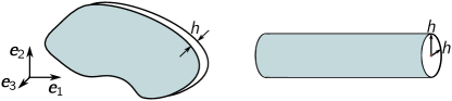
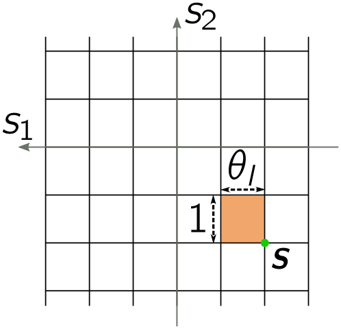
Consider a material domain , where is a 2-d domain in the plane spanned by , and is the material thickness in the normal direction (Fig. 1). Suppose , with on , is the dipole field in the material. The electrostatic energy density is given by
where is the volume of , and is the electric potential that satisfies the electrostatic equation
together with the constraint and the decay property
Let , and for be the map from to . For fixed , consider the dipole field and such that
Let be the sequence of dipole field for , and is defined as above. Assume that dipole field is such that, first, on , and, second, it converges to in ; then the limit of the energy density is [GJ97]:
That is, the limiting energy is local, and only the normal component of the dipole moment appears in the expression.
Next, consider a thin straight wire with axis along , denoted by , where is the ball of radius centered at in the plane spanned by (Fig. 1). Analogous to the thin film, let , on , be the dipole field in the material; be the rescaled domain of ; for be the map from to ; and be the rescaled dipole field defined as
| (2) |
The limiting energy density in the case of the thin wire is [CH15]:
where is the limiting dipole field. We notice that the limiting energy is again local, and only the components of the dipole moment perpendicular to the axis of the wire contribute.
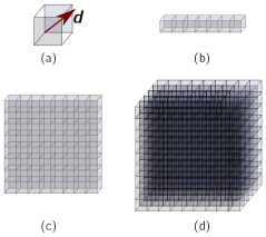
The absence of nonlocality in the limiting energy in the results above, as well as in our results in section 3 below, can be physically understood through the fact that these structures are 1-d or 2-d topologically. To see this, we consider a system of discrete dipoles associated with the uniform 1-d, 2-d, and 3-d periodic lattices with the unit cell of size (Figure 2). The energy of a lattice of dipoles is given by [Bro63, JM94]:
| (3) |
where the sum is over the cells in the lattice, and the term inside square bracket denotes the energy density of a cell . Here, denotes the unit cell; the measure (volume) of the unit cell ; the dipole in cell ; and, the coordinate of lattice site . The dipole field kernel, , is defined as:
| (4) |
We use these expressions to heuristically understand the scaling of the energy for systems with different topological dimensions. For simplicity, we assume below that the volume of the unit cell and the magnitude of the dipole are both , i.e., and for each , and some constant factors are neglected. For the next set of bounds, assume that and are generic positive constants.
Remark 2.1 (1-d lattice).
We can estimate an upper bound on the energy density of a typical unit cell as follows:
We use that the total dipole moment at a distance from a given unit cell is, at most, that of another dipole in the unit cell at a distance . This sum is well-behaved and bounded.
Remark 2.2 (2-d lattice).
As in the 1-d setting, we first bound the net dipole at a distance from a given unit cell. Since the structure is a 2-d lattice, the number of unit cells at a distance is of order . Therefore, an upper bound on the energy density is:
This sum is also well-behaved and bounded.
Remark 2.3 (3-d lattice).
Following the argument of the 2-d lattice, we now have that the net dipole at a distance from a given unit cell is, at most, of the order . Therefore, an upper bound on the energy density is:
This sum is divergent. However, through a more careful analysis that accounts for the signs – not just the magnitudes – of the dipole interactions, the energy density can be shown to be conditionally convergent111 That is, it is convergent, while the sums of only the positive terms and only the negative terms diverge, respectively, to . [Tou56, JM94].
When the lattice sum is bounded and converges unconditionally, it is possible to truncate after a finite distance and obtain sufficient numerical accuracy. When the lattice sum is conditionally convergent, that can be physically related to nonlocality; specifically, the slow convergence does not allow for truncation, and the far-field values play an important role. [MD14] discusses this from a physical perspective.
3 Results on Continuum Limits of the Electrostatic Energy
We consider two classes of nanostructures: helical nanotubes and thin films, the latter allowing for a constant bending curvature (i.e., nonzero constant mean curvature and zero Gauss curvature), and obtain the corresponding continuum limit electrostatic energy. In both cases, we start with discrete dipoles, where the discreteness is parametrized by the scale , and examine the limit . We show that the dipole-dipole interaction energy density – per unit cross-sectional area in the case of nanotubes, and per unit thickness in the case of films – converges to a local energy density in the limit.
3.1 Helical Nanotube
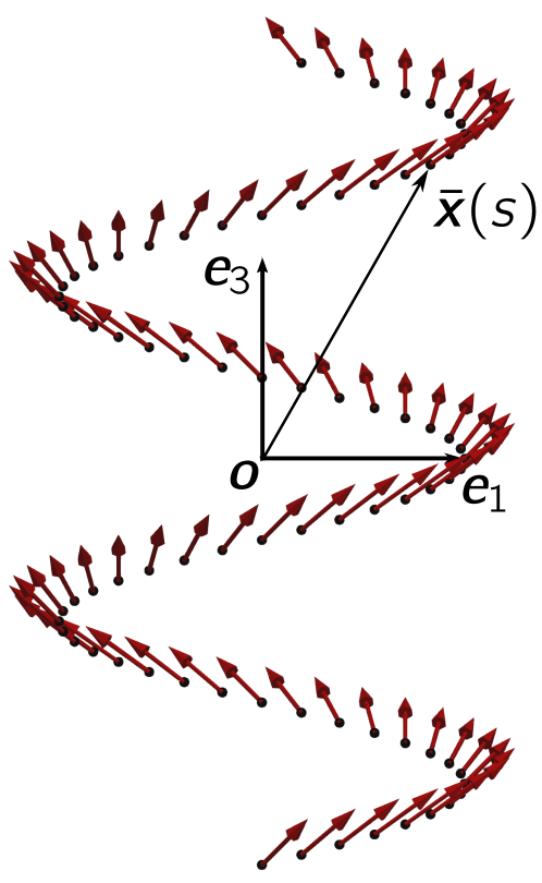
We consider a discrete helix with axis characterized by the angle and lengthscale ; the pitch of the helix is . Suppose is a point on the helix. Then, the other points on the helix are related by an isometric transformation of . Let be the parametric coordinate of a point on the helix. Then, the map that takes a point in the parametric space to a unique point on the helix can be expressed as
| (5) |
Here is the rotational tensor represented by the matrix in the orthonormal basis as:
| (6) |
Note that the definition of map imply that the helix makes a full turn in from , and, therefore, the pitch of the helix is .
Without loss of generality, we assume . The tangent vector to the helix at is given by
| (7) |
Let denote the unit tangent vector. We define the second order projection tensors and , for , as follows
| (8) |
For any vector and any , we have
| (9) |
3.1.1 Lattice Geometry and Dipole Moment
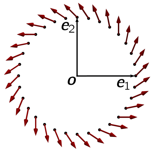
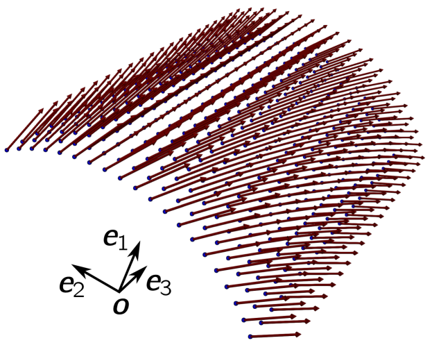
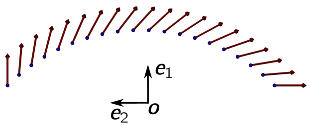
Let denote the set of parametric coordinates of the points on the helix. We consider a discrete system of dipole moments associated to the points on the helix given by (Figure 3). The magnitudes of the dipoles at the lattice sites are equal, but they are oriented differently; in particular, the orientations of dipoles at lattice sites follow the relation:
| (10) |
We associate a unit cell to each lattice site. Let denote the unit cell in the parametric space at the site , for . Let , , be given by
for some . Note that . The unit cell in real space is defined by . We take, without loss of generality, so that .
We now consider the setting in which the cells are of size , so that as the density of cells in the helix increases. For , suppose denotes the parametric coordinates of the sites in a scaled lattice, and denotes the corresponding system of dipole moments. Associated to , let denote the cell in the parametric space. The 3-d cell is given by , where is the scaled cross-section. Note that and . Let be the piecewise constant extension of given by
| (11) |
To compute the limit of the dipole-dipole interaction energy as , we assume that dipole moment density field converges to some field in the norm. As in [JM94], instead of working with , as defined above, we could assume that the dipole moment , for , is due to the background dipole moment density field such that
| (12) |
where is the area measure for surface . In the equation above, we assumed that the background field is uniform in for all and used . The existence of one such background field is evident: we can define . The physical dimension of is dipole moment per unit volume. We have the following lemma that relates the convergence of the background dipole moment field and the piecewise constant extension.
Lemma 3.1.
Let , , be the sequence of functions, and let be such that in . Let be given by (12), and be a piecewise constant extension of given by (11). Then, in .
On the other hand, if is such that in , then there exists a background field such that is given by (12).
The proof is similar to the proof of Theorem 4.1 from [JM94].
Remark 3.2.
Since the discrete dipole field has helical symmetry, from (12) we can see that will also have helical symmetry. However, we highlight that the background field needs to have helical symmetry only in the sense that the effective dipole has the helical symmetry, allowing for some fluctuations from site to site.
Remark 3.3.
The physical setting that we wish to examine is when dipole moments play a significant role in the limit. Therefore, we consider an appropriate scaling that corresponds to obtaining a finite limit for the dipole density field (or, equivalently, the background field, ). Further, we assume convergence in to ensure finite energies.
3.1.2 Electrostatic Energy
For , the energy associated to the system of dipole moments can be expressed as [Bro63, JM94]:
where is the energy per unit area given by
| (13) |
Substituting (12) into the expression above, and proceeding similar to Section 6 of [JM94], can be written as
| (14) |
where is the map given by
| (15) |
and , for , is the discrete dipole field kernel given by
| (16) |
Scaling of
For any , we have, using (5),
| (17) |
Using the relation above, it is easy to show that
where we recall that , , is the lattice cell in the parametric space for . Based on the equation above, we define a discrete kernel , for , as follows
| (18) |
We then have
3.1.3 Limit of the Electrostatic Energy
In this section, we obtain the limit of the energy per unit surface area as assuming that the background dipole field density (or equivalently the dipole moment density ) converges to some density field in . The idea is to first show that the map in (15) is bounded and obtain its limit. With that, the limit of follows.
Limit of the Discrete Electric Field
Let be the map with kernel . For any function , we have
| (19) |
We have the following main result on the map .
Proposition 3.4.
The maps and are bounded in for all and satisfy
| (20) |
Further, for ,
pointwise, where and are projection tensors that project onto the normal plane and the tangent line to the helix respectively (see (8)). Further, is a constant given by
| (21) |
We provide the proof of Proposition 3.4 in subsection 4.1.
Limit of the Energy
Theorem 3.5.
Proof 3.6.
Since is bounded and , we have
where the decomposition of the limit into the sum of individual limits is true if the two limits, and , individually exist. This is indeed true: because is bounded and in , we have that . Then, to show that exist for , we proceed as follows.
Let be a sequence of functions such that . Using Proposition 3.4, we have
| (22) |
where (see Proposition 3.4).
Remark 3.7.
The limiting energy only comprises of a local self-field energy. In the limit, any point on the helix sees a uniform 1-d system of dipole moments along the tangent line. Further, we see that both the normal components and the tangential component of the dipole moment contribute to the energy and electric field. This is in contrast to [CH15], where the thin wire limit of the magnetostatic energy, obtained from dimensional reduction starting from a 3-d continuum, has contributions only from the normal component. Heuristically, the dimension reduction starting from a 3-d continuum contains minimal information about the detailed atomic arrangements within the nanostructure, and hence does not capture the consequences of the helical geometry. Because of its starting point in a 3-d continuum model, it is appropriate for thin objects that have all dimensions being much larger than the atomic lengthscale. On the other hand, the discrete-to-continuum approach is appropriate for nanostructures wherein the thin dimension is comparable to the atomic lengthscale.
3.2 Nanofilm with Constant Bending Curvature
Let be the parametric space for a surface with a constant bending curvature . The map that takes a point in the parametric space to a unique point on the film is given by
| (24) |
where is the inverse of curvature, is the angular size of the film, and is the spacing in the flat direction. Here, are fixed parameters for a given film. Here, is the rotational tensor with the axis , see definition (6). The tangent vectors at are
| (25) |
and the normal vector is
| (26) |
3.2.1 Lattice Geometry and Dipole Moment
We consider a lattice embedded on the film . We assume that the film is one lattice cell thick in the direction normal to the film. Suppose is the set of parametric coordinates of the discrete lattice sites. Let and the lattice cell (in the parametric space ) be given by
| (27) |
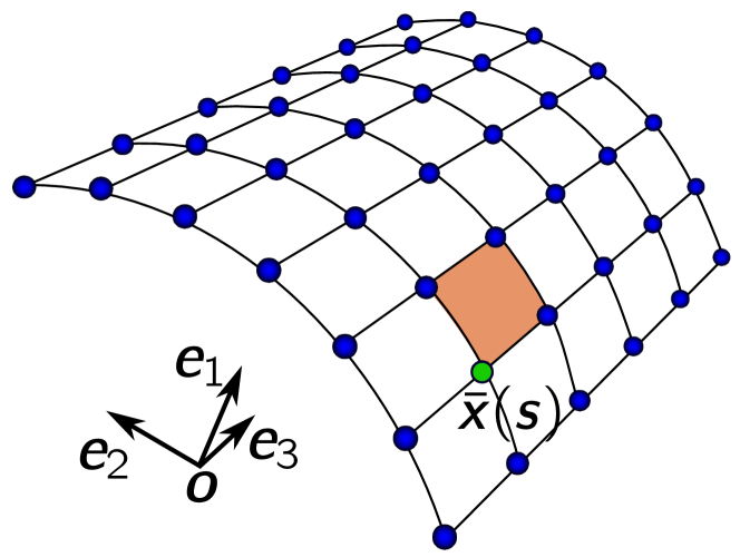
Here, is the angular width of the lattice cell. We assume that is such that the set of sites in the angular direction, , is not empty, and in fact is sufficiently large so that the continuum limit approximation of the energy density is justified. We assume that the lattice has unit thickness in the normal direction, and suppose that the film given by passes through the center of the lattice in the normal direction. Then, the unit cell for a given site is (see Fig. 4). On the lattice , we define a discrete system of dipole moments . As in the case of the helical nanotube, the lattice cells in real space are related by an isometric transformation, so the magnitudes of the dipoles at the lattice sites are equal, but they are oriented differently. In particular, we have
| (28) |
where such that (i.e. all the translations within ). We see that the dipole orientation depends only on the angular (first) parameter and is invariant with respect to the second parameter.
We next consider the scaling of the lattice by . The scaled lattice and the associated lattice cell are defined by the natural scaling of and as follows
| (29) |
After scaling, the thickness of the lattice cell in the normal direction is and the unit cell for is . We can show that the unit cell in the scaled lattice has volume . Let denote the discrete system of dipole moments associated with the scaled lattice, , and denote the piecewise constant extension of given by
| (30) |
We are interested in the limit of the energy when converges to in . As in the case of the helix and following [JM94], we suppose that there exists a background dipole moment density field such that the dipole moment at site is given by
| (31) |
where is the area measure (note that does not include ). The existence of one such background field is evident: we can define . Similar to the case of the helix, we have the following lemma that relates the convergence of the background dipole moment field and the piecewise constant extension.
Lemma 3.8.
Let , , be a sequence of functions and let be such that in . Let be given by (31) and let be a piecewise constant extension of given by (30). Then, in .
On the other hand, if is such that in , then there exists a background field such that is given by (31).
The proof follows directly from the proof of Theorem 4.1 of [JM94].
Remark 3.9.
As different unit cells are related by isometric transformations, the dipole moments in different unit cells are related by the rotational part of the isometric transformation.
3.2.2 Electrostatic Energy
As before, the energy associated to the system of dipole moments , for , is given by
where is the thickness of the lattice in normal direction, and is the energy per unit length given by
| (32) |
For convenience, we normalize by , where is independent of and gives the size of the original lattice in the angular direction. We let
| (33) |
Substituting (31) and proceeding similar to the case of the helix, we can express as
| (34) |
where is the map defined as
| (35) |
and , for , is the discrete dipole field kernel given by
| (36) |
Scaling of
As in the case of the helix, it is convenient to first rescale the lattice such that the lattice cell size is independent of after rescaling, and define a new map on the rescaled lattice. This is considered next.
Let so that implies . We define a rescaled lattice such that implies . It is given by
| (37) |
The lattice cell for is given by , where is defined in (27) (using in ). For , we have
| (38) |
where
| (39) |
Keeping in mind these definitions, for , we also note
| (40) |
Using the above relation and (38), we can show, for any ,
If we introduce the discrete dipole field kernel , for , defined on as:
| (41) |
we have shown that:
3.2.3 Limit of the Electrostatic Energy
In this section, we obtain the limit of the energy per unit length . The broad strategy is similar to the helical nanotube. We first show that the map is bounded and obtain its limit. The continuum limit of the energy density then follows easily.
Limit of the Discrete Electric Field
Let be the map with kernel . For any function , we have
| (42) |
Let be the zeroth order moment (with respect to the first argument) of kernel given by
| (43) |
We now state the limit result of .
Proposition 3.10.
Suppose . The maps and are bounded in for all and satisfy
Further, for ,
pointwise, where , for , is given by
| (44) |
and , , are the tangent vectors to the film.
We provide the proof of Proposition 3.10 in subsection 4.2. Based on the proposition above, we state the main result for the thin film.
Limit of the Energy
Theorem 3.11.
Let be a sequence of functions for with such that in . Let the system of dipole moments be given by (31). Let , given by (34), be the energy per unit length normalized by . Then
where is defined in Proposition 3.10, see (44).
The proof of Theorem 3.11 follows from the proof of Theorem 3.5 and using Proposition 3.10.
Remark 3.12.
Note that, for ,
| (45) |
Thus, if the limiting dipole moment field is uniform in the direction, the electric field will be independent of the -coordinate. It is easy to see from the expression of that both the normal component and the tangential components of the dipole field contribute to the electric field and energy. This is in contrast to [GJ97], where the thin film limit of the magnetostatic energy, obtained from dimensional reduction starting from a 3-d continuum, has contributions only from the normal component. However, it is consistent with the result for the helical nanostructure studied in this paper, in that the components of the dipole field aligned with the thin direction contribute to the limit energy. As we argued there, the dimensional reduction from a 3-d continuum model is appropriate for thin films that have thickness that is much larger than the atomic lengthscale, whereas the discrete-to-continuum approach is appropriate for nanostructures that have thickness that is comparable to the atomic lengthscale.
4 Proof of Assertions
4.1 Helical Nanotube
In this section, we prove Proposition 3.4. First, we collect some important results, and then show that is bounded and extends from to . We then obtain the limit of the map .
Lemma 4.1.
- 1.
-
2.
For any ,
(47) where is for .
-
3.
For any and ,
(48) where is given by
-
4.
For any such that , suppose are such that , then
(49)
Proof 4.2.
- 1.
- 2.
- 3.
-
4.
To show (49), we note that for such that with and , we can write and with . Thus
where in the last step we used the fact that for (which is ensured when ).
This completes the proof.
4.1.1 Boundedness
We next show that is a bounded map. Let be an isometry defined as
It is easy to see that . The inverse of is given by
| (52) |
Using , we can show – noting the definition of in (15) – for ,
| (53) |
where we used a change of variables and (52). It follows from the above equation that
| (54) |
where we have used that . This completes the proof of (20) in Proposition 3.4. Next, we show that is a bounded map to prove the boundedness of . We first analyze the discrete dipole field kernel , which is defined as
| (55) |
where for , and is given by (17).
Consider some typical and the corresponding such that . From (55), we have, for all such that ,
-
•
If , then .
- •
Combining the two cases above, .
We now consider the case when . Noting that for this case, . We proceed as follows
| (56) |
where we used the bounds (48) and (49). Combining the above bound for with the bound for , and renaming the constants, we can write
| (57) |
Next, note that, since the kernel satisfies (57), we have
| (58) |
for some fixed independent of . Using the above bound, we can show that, for all ,
| (59) |
which establishes that is a bounded linear map on . Since is dense in , it follows that is also bounded in , and extends as a bounded linear map from to . This argument together with (54) completes the proof of boundedness of maps and . Now, it remains to show (59) for . Let and proceed as follows:
| (60) |
where, in the third line we have used that ; in the fourth line, we have used symmetry to extract a factor of ; in the last line, we have used the bound (58). Since , there exist such that the support of is a subset of . So, for any , we have
| (61) |
where we have applied Fubini’s theorem to switch the order of integration – this is allowed because is integrable in – and then used (58). Thus, we have shown that is bounded, with the bound independent of . This, together with the fact that is monotonically increasing with , shows that exists and is equal to , where is defined in (60). The limit is also bounded, i.e., . Combining this observation with (60) completes the proof of (59).
4.1.2 Limit of the Map
Let . Write as:
| (62) |
The second term above is zero in the limit . To see this, we first obtain two useful inequalities. For any , we have, using the bound on from (57),
| (63) |
and
| (64) |
where the last equality in the equation above follows from the change of variables . Next, noting that , we obtain the following bound on the second term of (62):
| (65) |
where we have used the fact that , and therefore, , and for . We have also used the inequalities (63) and (64) in the last step.
We note that the final inequality in (65) is true for any . Further, the two terms on the right side have a limit as – the second term clearly is independent of – for any . Therefore, the limit of the two terms individually is equal to the limit of the sum, keeping fixed. Thus, taking the limit in (65), we have
| (66) |
for any . Since the bound above is true for any , and the left side is independent of , we can take the limit , where the limit exists and is for the right side, to get
| (67) |
Thus, we have from (62) that
| (68) |
We next compute the limit of . Fix and suppose such that . Using the definition of , we have
| (69) |
From (50), we have . Using the identity and , we get
| (70) |
where we have changed variables . Note that , and, therefore, for , which implies . Since is related to by , we have in the limit . Therefore, we get
To take the limit inside the summation, we show that the sum is absolutely convergent for all as follows:
| (71) |
Now, we can write
Note that for a fixed
where . Now, using the equation above, and the fact that is smooth away from (which is ensured in the summation), we get
Combining this with (68), we get
Next, we simplify . Using and , we can show
| (72) |
where is the tangent vector, and with . In (72), by noting the definition of the dipole field kernel , it is easy to show that
with defined as
| (73) |
and projection tensors and . This finishes the proof of Proposition 3.4.
4.2 Nanofilm with Uniform Bending
In this section, we prove Proposition 3.10. The outline of the proof is similar to the case of the helix in subsection 4.1.
Lemma 4.3.
-
1.
Suppose such that with . When , we have and
(74) - 2.
Proof 4.4.
To show (74), we proceed as follows. For and corresponding , there exists such that with , . We have the bound
| (76) |
where in the last step we used the fact that any , satisfying , are at least distance apart.
We next show (75). Using
and
we have that
| (77) |
Let . Then, using a Taylor expansion and the mean value theorem, there exists such that
Since , it follows
Substituting the relation above in (77), we get
Since , we have , and
Using the two equations above and defining the constant as in Lemma 4.3(2), (75) can be easily shown.
4.2.1 Boundedness
Let be a map such that, for any ,
It is easy to see that is an isometry. The inverse of is given by
Following the similar steps in subsubsection 4.1.1, we can show that
Thus, to show that is a bounded map, it is sufficient to show that is bounded. Towards that goal, we first establish that
| (78) |
where are constants that may depend on the parameters defining the surface , but are independent of .
To show (78), we recall that is the fixed angular extent of the film and satisfies the bound (in fact we restrict it such that ). Let be any two generic points, and let be such that and . We refer to subsubsection 3.2.1 and subsubsection 3.2.2 for the notation appearing in this section.
First, consider such that . For this case, we have . Noting that , , we have
| (79) |
Next, we consider the case when . This can be further divided in two cases:
-
•
Case 1: which implies .
-
•
Case 2: . For this case, we have
(80) Note that when , we can have either ; or ; or . For all of these cases, the denominator in (80) is bounded from below because . Thus, we have
(81)
In summary (81) holds for any such that .
Combining the bound for the case with the bound for the case , we can write
| (82) |
where we have renamed the constants for convenience. This completes the proof of (78).
Next, we show is a bounded map on . Since satisfies (78), it can be shown that
| (83) |
for some fixed independent of . Following the steps in obtaining inequality (60), it is easy to obtain, for ,
| (84) |
Let , and let is defined as
| (85) |
where is the two-dimensional ball of radius centered at . Based on the arguments in the last paragraph of subsubsection 4.1.1, we find that exist and it is given by , where is defined in (84), and that the limit satisfies the bound . Combining this with (84), we have shown that, for ,
Arguing as in the case of the helix, the map is a bounded linear map on .
4.2.2 Limit of the Map
Let . We write as follows
| (86) |
We next show that the second term in (86) is zero in the limit . Fix , then we have
| (87) |
where, in the last step, we have used that , and, for , we have . To bound and , first observe that, due to and the bound on in (82), there holds
| (88) |
and as a direct consequence, we have
| (89) |
where, in the second step, the domain of integration was enlarged; and, in the final step, the change of variables (so that ) was introduced. Next, using the definition of in (87) and (88), we get
| (90) |
where, in the second step, the domain of integration was enlarged; in the third step, the change of variables was introduced; and, finally, in the last step, was used. Combining the results of (89) and (90) with (87), we have shown that
| (91) |
for any . Arguing as in the case of helix – see the discussion associated with (67) – we have
for any . We can take the limit of both sides above since the inequality is valid for any , and the left side is independent of and the limit of of the right side is well-defined and equal to . We have therefore shown
Thus, from (86), we have
| (92) |
Limit of
Consider a typical such that where . Recall that is the lattice for and is the lattice cell. In the definition of , we substitute , to get
| (93) |
Substituting the definition of transformation in (24), we can show for that
Using the identities and , from (93), we have
| (94) |
We analyze as follows. First, we expand the sum
| (95) |
where we introduced the new variable . Since , we have . Using a Taylor expansion and the mean value theorem, we have the identity
| (96) |
where depends on . Formula (96) suggests that we decompose (95) as:
| (97) |
Step 1: We show goes to zero in the limit . Let
| (98) |
Consider a function defined as
| (99) |
Note that, since and , we have
| (100) |
We show that and the lower bound is independent of . For convenience, let . Since , and , we have . The hypothesis of Proposition 3.10 restricts such that
| (101) |
With , writing out the action of and on , we get
| (102) |
Through elementary calculations, we can show
| (103) |
Using a Taylor expansion and noting that , there exists with such that
| (104) |
Thus
| (105) |
where we used the fact that in the fourth line, and is the minimum with respect to of the function in the square bracket in the fifth line. Further, since , we have
| (106) |
for any and . The lower bound on is independent of and . Finally, combining (106) with (100), we get
| (107) |
Proceeding further, we have, from the fundamental theorem of calculus,
| (108) |
Note that because of (107), exists and is bounded. From the definition of in (97), a change of variable , the definition of in (98) and (102), and noting the identity (108), we have
| (109) |
where we used the bound on the gradient of with constant fixed.
Next, we get an upper bound on in terms of . From (102), we have
By a Taylor expansion and the mean value theorem, we have where depends on . Substituting this and using the bound , we obtain
| (110) |
Combining the equation above with (109), we get
| (111) |
where in the third line we introduced the variable . We only have to show that the term inside the braces is bounded as to conclude that as . First, note from (105), we have
| (112) |
Therefore,
| (113) |
Thus
| (114) |
Note that the integrand is independent of . Further, the numerator has whereas the denominator has , therefore, the sum inside the braces is absolutely convergent and finite. Hence, due to the factor , we have shown .
This completes Step 1. We next study .
Step 2: We have from (97)
| (115) |
where we have used the notation to denote the set . Using the decay property of the dipole field kernel , we can show that in the limit . Therefore, we have
| (116) |
where we introduced the new variable . Since and , we have . This completes Step 2. Note that is independent of .
Upon substituting the limit of and in (97), we have shown
| (117) |
Recall that was fixed such that , which implies that as . With this observation and (117), we have from (94),
| (118) |
Next we simplify . Given the parametric map , the two tangent vectors at are
| (119) |
Using and , we write,
This completes the proof of Proposition 3.10.
5 Summary of Results
We have shown rigorously that certain low-dimensional nanostructures do not have long-range dipole-dipole interaction in the continuum limit. The energy density in the limit is entirely because of the Maxwell self-field. In 1-d and 2-d lattices (in a 3-d ambient space), the dipole field kernel decay is sufficiently fast that long-range interactions do not contribute to the limit energy.
While our calculations show that the energy is local in the continuum limit for 1-d and 2-d discrete systems, in agreement with dimension reduction approaches that reduce a 3-d continuum to a 1-d or 2-d continuum (e.g., [GJ97, CH15] and others), we note an interesting difference. As shown in [GJ97] and other work following it, the component of the dipole moment along the normal direction to the film is the only contributor to the continuum electrostatic energy in the thin film limit. Similarly, [CH15] show that the component of the dipole moment in the plane normal to the wire is the only contributor to the continuum electrostatic energy in the thin wire limit.
This is different from the limit energy in the discrete-to-continuum limit obtained in this work: for the case of a helical nanotube, the limiting energy density is given by (see Theorem 3.5)
where is a constant, and and are, respectively, the projections of the dipole moment field along the axis of the helix and in the plane normal to the axis of the helix. Therefore, unlike the thin wire limit using dimension reduction, the discrete-to-continuum energy has contributions from both the normal and tangential components of the dipole moment field. For the case of a thin film with curvature, the limiting energy density is given by (see Theorem 3.11)
where
Here, is the parametric domain of the film, is the inverse of the curvature, is the angular width of the unit cell, and , , are the tangent vectors at coordinate . For simplicity, we fix and assume and ; then the lattice sum above is over a 2-d lattice in plane. By substituting the form of and computing , we can show that both the normal and the tangential components of are present in the final expression for the energy above.
We can understand these differences physically, by first noticing that the dimension reduction starting from the 3-d continuum contains minimal information about the detailed geometry of the underlying lattice within the nanostructure; these approaches have 3-d continuum theory as their starting point, and are valid for situations in which the limiting thin object has all dimensions much larger than the atomic lengthscale. In contrast, the discrete-to-continuum approach presented here is appropriate for nanostructures in which the thin dimensions are comparable to the atomic lengthscale. For this reason, the thin-film model obtained in this work may capture better the electromechanics of lipid bilayers, as these are composed of only 1-2 unit cells in the thickness direction [LS13, ADLS13, TMLS22, Ste18].
Acknowledgments
This paper draws from the doctoral dissertation of Prashant K. Jha at Carnegie Mellon University [Jha16]. We thank Richard D. James for useful discussions; AFRL for hosting a visit by Kaushik Dayal; and NSF (2108784, 1921857), ARO (W911NF-17-1-0084), ONR (N00014-18-1-2528), and AFOSR (MURI FA9550-18-1-0095) for financial support.
References
- [ABC08] Roberto Alicandro, Andrea Braides, and Marco Cicalese. Continuum limits of discrete thin films with superlinear growth densities. Calculus of Variations and Partial Differential Equations, 33(3):267–297, 2008.
- [ACG08] Roberto Alicandro, Marco Cicalese, and Antoine Gloria. Variational description of bulk energies for bounded and unbounded spin systems. Nonlinearity, 21(8):1881, 2008.
- [ACG11] Roberto Alicandro, Marco Cicalese, and Antoine Gloria. Integral representation results for energies defined on stochastic lattices and application to nonlinear elasticity. Archive for rational mechanics and analysis, 200(3):881–943, 2011.
- [ADE13a] Amin Aghaei, Kaushik Dayal, and Ryan S Elliott. Anomalous phonon behavior of carbon nanotubes: First-order influence of external load. Journal of Applied Physics, 113(2):023503, 2013.
- [ADE13b] Amin Aghaei, Kaushik Dayal, and Ryan S Elliott. Symmetry-adapted phonon analysis of nanotubes. Journal of the Mechanics and Physics of Solids, 61(2):557–578, 2013.
- [ADLS13] F Ahmadpoor, Q Deng, LP Liu, and P Sharma. Apparent flexoelectricity in lipid bilayer membranes due to external charge and dipolar distributions. Physical Review E, 88(5):050701, 2013.
- [ALP18] Roberto Alicandro, Giuliano Lazzaroni, and Mariapia Palombaro. Derivation of a rod theory from lattice systems with interactions beyond nearest neighbours. Networks & Heterogeneous Media, 13(1):1, 2018.
- [BBC20] Annika Bach, Andrea Braides, and Marco Cicalese. Discrete-to-continuum limits of multibody systems with bulk and surface long-range interactions. SIAM Journal on Mathematical Analysis, 52(4):3600–3665, 2020.
- [BLBL02] Xavier Blanc, Claude Le Bris, and P-L Lions. From molecular models to continuum mechanics. Archive for Rational Mechanics and Analysis, 164(4):341–381, 2002.
- [BLBL07] Xavier Blanc, Claude Le Bris, and Pierre-Louis Lions. Atomistic to continuum limits for computational materials science. ESAIM: Mathematical Modelling and Numerical Analysis, 41(2):391–426, 2007.
- [Bro63] William Fuller Brown. Micromagnetics. Number 18. interscience publishers, 1963.
- [Car01] Gilles Carbou. Thin layers in micromagnetism. Mathematical Models and Methods in Applied Sciences, 11(09):1529–1546, 2001.
- [CDZ09] Marco Cicalese, Antonio DeSimone, and Caterina Ida Zeppieri. Discrete-to-continuum limits for strain-alignment-coupled systems: magnetostrictive solids, ferroelectric crystals and nematic elastomers. Networks & Heterogeneous Media, 4(4):667, 2009.
- [CH15] Khaled Chacouche and Rejeb Hadiji. Ferromagnetic of nanowires of infinite length and infinite thin films. Zeitschrift für angewandte Mathematik und Physik, 66(6):3519–3534, 2015.
- [DJ07] Traian Dumitrică and Richard D James. Objective molecular dynamics. Journal of the Mechanics and Physics of Solids, 55(10):2206–2236, 2007.
- [DLO10] Matthew Dobson, Mitchell Luskin, and Christoph Ortner. Sharp stability estimates for the force-based quasicontinuum approximation of homogeneous tensile deformation. Multiscale Modeling & Simulation, 8(3):782–802, 2010.
- [FJ00] Gero Friesecke and Richard D James. A scheme for the passage from atomic to continuum theory for thin films, nanotubes and nanorods. Journal of the Mechanics and Physics of Solids, 48(6-7):1519–1540, 2000.
- [GD20a] Matthew Grasinger and Kaushik Dayal. Architected elastomer networks for optimal electromechanical response. Journal of the Mechanics and Physics of Solids, page 104171, 2020.
- [GD20b] Matthew Grasinger and Kaushik Dayal. Statistical mechanical analysis of the electromechanical coupling in an electrically-responsive polymer chain. Soft Matter, 2020.
- [GH15] Antonio Gaudiello and Kamel Hamdache. A reduced model for the polarization in a ferroelectric thin wire. Nonlinear Differential Equations and Applications NoDEA, 22(6):1883–1896, 2015.
- [GJ97] Gustavo Gioia and Richard D James. Micromagnetics of very thin films. Proceedings of the Royal Society of London. Series A: Mathematical, Physical and Engineering Sciences, 453(1956):213–223, 1997.
- [HTJ12] Ye Hakobyan, Ellad B Tadmor, and Richard D James. Objective quasicontinuum approach for rod problems. Physical Review B, 86(24):245435, 2012.
- [Jam06] Richard D James. Objective structures. Journal of the Mechanics and Physics of Solids, 54(11):2354–2390, 2006.
- [Jha16] Prashant Jha. Coarse Graining of Electric Field Interactions with Materials. PhD thesis, Carnegie Mellon University, 2016.
- [JM94] Richard D James and Stefan Müller. Internal variables and fine-scale oscillations in micromagnetics. Continuum Mechanics and Thermodynamics, 6(4):291–336, 1994.
- [KO01] J Knap and M Ortiz. An analysis of the quasicontinuum method. Journal of the Mechanics and Physics of Solids, 49(9):1899–1923, 2001.
- [KS05] Robert V Kohn and Valeriy V Slastikov. Another thin-film limit of micromagnetics. Archive for rational mechanics and analysis, 178(2):227–245, 2005.
- [KSZ15] Martin Kružík, Ulisse Stefanelli, and Chiara Zanini. Quasistatic evolution of magnetoelastic plates via dimension reduction. Discrete & Continuous Dynamical Systems-A, 35(12):5999, 2015.
- [LLO12] Xingjie Helen Li, Mitchell Luskin, and Christoph Ortner. Positive definiteness of the blended force-based quasicontinuum method. Multiscale Modeling & Simulation, 10(3):1023–1045, 2012.
- [LPS15] Giuliano Lazzaroni, Mariapia Palombaro, and Anja Schlömerkemper. A discrete to continuum analysis of dislocations in nanowire heterostructures. Communications in Mathematical Sciences, 13(5), 2015.
- [LPS17] Giuliano Lazzaroni, Mariapia Palombaro, and Anja Schlömerkemper. Rigidity of three-dimensional lattices and dimension reduction in heterogeneous nanowires. Discrete and Continuous Dynamical Systems - S, 10(1):119–139, 2017.
- [LS13] LP Liu and P Sharma. Flexoelectricity and thermal fluctuations of lipid bilayer membranes: Renormalization of flexoelectric, dielectric, and elastic properties. Physical Review E, 87(3):032715, 2013.
- [MD14] Jason Marshall and Kaushik Dayal. Atomistic-to-continuum multiscale modeling with long-range electrostatic interactions in ionic solids. Journal of the Mechanics and Physics of Solids, 62:137–162, 2014.
- [MS02] Stefan Müller and Anja Schlömerkemper. Discrete-to-continuum limit of magnetic forces. Comptes Rendus Mathematique, 335(4):393–398, 2002.
- [MT02] Ronald E Miller and Ellad B Tadmor. The quasicontinuum method: Overview, applications and current directions. Journal of Computer-Aided Materials Design, 9(3):203–239, 2002.
- [Sch05] Anja Schlömerkemper. Mathematical derivation of the continuum limit of the magnetic force between two parts of a rigid crystalline material. Archive for rational mechanics and analysis, 176(2):227–269, 2005.
- [Sch06] Bernd Schmidt. A derivation of continuum nonlinear plate theory from atomistic models. Multiscale Modeling & Simulation, 5(2):664–694, 2006.
- [Sch08] Bernd Schmidt. On the passage from atomic to continuum theory for thin films. Archive for rational mechanics and analysis, 190(1):1–55, 2008.
- [Sch09] Bernd Schmidt. On the derivation of linear elasticity from atomistic models. Networks & Heterogeneous Media, 4(4):789, 2009.
- [SS09] Anja Schlömerkemper and Bernd Schmidt. Discrete-to-continuum limit of magnetic forces: dependence on the distance between bodies. Archive for rational mechanics and analysis, 192(3):589–611, 2009.
- [Ste18] David J Steigmann. Mechanics and physics of lipid bilayers. In The role of mechanics in the study of lipid bilayers, pages 1–61. Springer, 2018.
- [SWB+21] Shoham Sen, Yang Wang, Timothy Breitzman, , and Kaushik Dayal. Two-scale analysis of the polarization density in ionic solids. in preparation, 2021.
- [TM11] Ellad B Tadmor and Ronald E Miller. Modeling materials: continuum, atomistic and multiscale techniques. Cambridge University Press, 2011.
- [TMLS22] Mehdi Torbati, Kosar Mozaffari, Liping Liu, and Pradeep Sharma. Coupling of mechanical deformation and electromagnetic fields in biological cells. Reviews of Modern Physics, 94(2):025003, 2022.
- [TOP96] Ellad B Tadmor, Michael Ortiz, and Rob Phillips. Quasicontinuum analysis of defects in solids. Philosophical magazine A, 73(6):1529–1563, 1996.
- [Tou56] Richard A Toupin. The elastic dielectric. Journal of Rational Mechanics and Analysis, 5(6):849–915, 1956.
- [Xia05] Yu Xiao. The influence of oxygen vacancies on domain patterns in ferroelectric perovskites. PhD thesis, California Institute of Technology, 2005.