for the Hadron Spectrum Collaboration

Constraining the quark mass dependence of the lightest resonance in QCD

Abstract

Lattice QCD spectra can be used to constrain partial-wave scattering amplitudes that, while satisfying unitarity, do not have to respect crossing symmetry and analyticity. This becomes a particular problem when extrapolated far from real energies, e.g. in the case of broad resonances like the $\sigma$, leading to large systematic uncertainties in the pole position. In this letter, we will show how dispersion relations can implement the additional constraints, using as input lattice–determined $\pi\pi$ partial wave scattering amplitudes with isospin–0,1,2. We will show that only certain combinations of amplitude parameterizations satisfy all constraints, and that when we restrict to these, the $\sigma$ pole position is determined with minimal systematic uncertainty. The evolution of the now well-constrained $\sigma$ pole with varying light quark mass is presented, showing how it transitions from a bound-state to a broad resonance.

Introduction — Pion-pion scattering with isospin–0 plays a key role in nuclear and particle physics, with the $J^{P}=0^{+}$ component proving to be a feature of many low-energy phenomena of contemporary interest such as spontaneous symmetry breaking [1], the long-range nucleon-nucleon interaction [2], and hadronic contributions to the anomalous magnetic moment of the muon [3]. At low energies, this partial wave is dominated by the existence of the $\sigma$ particle, the lightest resonance in Quantum Chromodynamics (QCD). This extremely short-lived state which manifests as a slow energy variation of the scattering amplitude, has only had its complex energy plane pole position pinned down precisely relatively recently [4, 5, 6]. How this state arises within QCD, and its relationship to other light-scalar mesons, like the $\kappa$, the $f_{0}(980)$, and the $a_{0}(980)$, remains unclear.

Our leading tool to study non-perturbative aspects of QCD, including hadron scattering and resonances, is Lattice QCD. This is a first-principles numerical approach in which only controlled approximations are made, and which features the ability to vary the value of quark masses and to explore the evolution of physical observables with such variation. Access to scattering amplitudes comes via computation of the discrete spectrum of states in the finite-volume of the lattice, extracted from the time-dependence of Euclidean correlation functions. A finite-volume quantization condition often referred to as the Lüscher equation, relates the spectrum to infinite-volume partial-wave scattering amplitudes [7, 8, 9, 10, 11, 12, 13, 14, 15, 16, 17, 18]. In practice, the computed spectra are used to constrain unitarity-satisfying parameterizations of the isospin–0 $S$–wave partial-wave amplitude, which when analytically continued in the complex energy plane, yield the $\sigma$ pole [19, 20, 21].

With light quark masses chosen so that the pion has a mass of 391 MeV, the $\sigma$ appears as a well-determined stable bound-state pole below the $\pi\pi$ threshold. On the other hand, in calculations at a pion mass of 239 MeV it was found that a wide range of parameterizations were capable of describing the finite-volume spectrum, all giving compatible amplitude determinations across the elastic scattering region, but these various amplitudes feature resonant $\sigma$ pole positions lying deep in the complex plane which are scattered well outside the level of statistical uncertainty [19].

This observation is closely related to the longstanding challenge of accurately determining the $\sigma$ pole position from fits to experimental $\pi\pi$ elastic scattering data [22]. In that case, a solution was found using dispersion relations which implement the additional fundamental constraint of crossing symmetry, leading to precise contemporary estimates of the $\sigma$ pole position [4, 5, 6, 23].

In this letter we will apply dispersion relations to lattice QCD data, considering two unphysical values of the light quark mass lying in the region where we believe the $\sigma$ is transitioning from being bound into being a broad resonance, showing that the dominant systematic error on the $\sigma$ pole position associated with parameterization of partial-wave scattering amplitudes can be almost entirely removed. Combining these results with calculations at heavier quark masses, we present the first robust estimation within first-principles QCD of the evolution of the $\sigma$ pole with varying quark mass.

The Hadron Spectrum Collaboration has performed lattice calculations yielding discrete finite-volume spectra in channels with the quantum numbers of $\pi\pi$ scattering for four values of the light quark mass, corresponding to pion masses of $391,330,283$ and $239$ MeV [24, 25, 26, 27, 19, 28, 29]. The $\pi\pi$ elastic partial-wave scattering amplitudes constrained using these spectra feature a $\rho$ in the isovector $P$–wave that is a resonance at all quark masses, while the isoscalar $S$–wave has an accurate interpretation only for the heaviest two quark masses, where the $\sigma$ appears as a well-determined bound-state pole.

In this letter we will focus on the lightest two quark masses. In both these cases, the $I=2$ $S$–wave amplitude ($S2$) is weak, repulsive, and decently described over the elastic region by a scattering length approximation. The $I=2$ $D$–wave ($D2$) is extremely weak across the elastic region. The $I=1$ $P$–wave ($P1$) is dominated by the narrow $\rho$ resonance, which is well described by a Breit-Wigner amplitude, while the $F$–wave is completely negligible. The $I=0$ $S$–wave amplitude ($S0$) at both quark masses is a slowly varying function of energy, but there is a significant change in the behavior at threshold between the two quark masses, indicating a rapid variation in the scattering length with the quark mass.

The $S0$ ‘lattice data’ (at both quark masses) proves to be describable by a large variety of unitarity-respecting parameterization forms, and these various descriptions lead to a spread of $\sigma$ pole estimates, with a scatter much larger than their statistical uncertainties. For the lightest pion mass, this is illustrated in Figure 3 (gray points). It is clear, then, that the lattice data in $S0$ alone, even when it has rather small statistical errors, does not provide sufficient constraint to uniquely determine the $\sigma$ pole position. We will use the additional constraint of crossing symmetry, in the form of dispersion relations applied to the coupled system of lattice data in all the partial waves above, to pin down the location of the $\sigma$ pole at $m_{\pi}\sim 283$ and $239$ MeV .

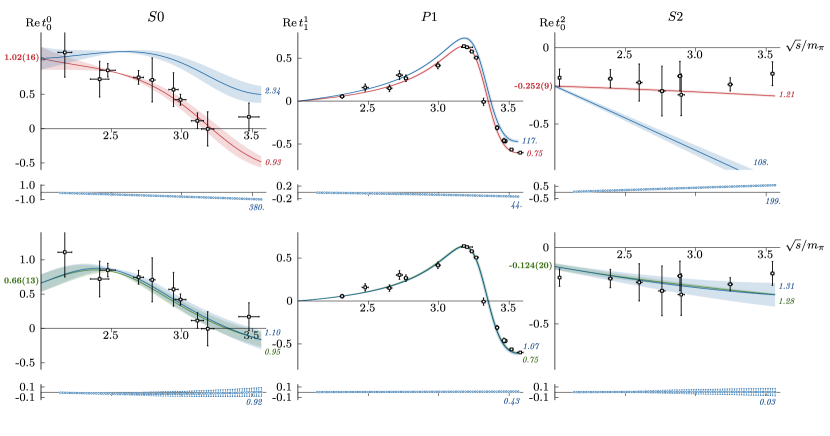
Figure 1: Real parts of $S0$, $P1$, $S2$ scattering amplitudes for $m_{\pi}\sim 239$ MeV. Data-points indicate the constraint provided by discrete lattice QCD spectra. The upper row shows an example of parameterizations (red) which describe well the lattice data, but which generate dispersed amplitudes (blue) that are in poor agreement, leading to large values of $d^{2}$ and $\tilde{\chi}^{2}$. The lower row shows a case where the lattice amplitudes (green) prove to be in good agreement with the dispersed amplitudes. The colored numbers with an error estimate represent the different scalar scattering lengths. The red(green) italic numbers represent the $\tilde{\chi}^{2}/N_{\text{lat}}$ values for the fits to the data, whereas the blue numbers on those same panels represent the dispersive $\tilde{\chi}^{2}/N_{\text{lat}}$ value. Beneath each panel, values of the quantity in the large parentheses in Eq. 2 at $N_{\mathrm{smpl}}=85$ points are given, and the numbers listed there represent the $d^{2}/N_{\text{smpl}}$ values.

Dispersion relations — Generically, crossing symmetry relates two-particle scattering behavior in the $s,t$ and $u$–channels in terms of the same amplitude, $T(s,t,u)$, evaluated in different kinematical regions. But this fundamental symmetry is obscured when the amplitude is partial-wave projected in one channel, e.g. $t_{\ell}(s)=\tfrac{1}{64\pi}\int\!d\!\cos\theta_{s}\,T(s,t,u)\,P_{\ell}(\cos\theta_{s})$, with the scattering dynamics in the $t$ and $u$–channels appearing as a left-hand cut, i.e. as an imaginary part of $t_{\ell}(s)$ for $s<0$. When the only constraint on the partial-wave amplitude is data for $s>s_{\mathrm{thr}}$, typically the left-hand cut remains undetermined.

In the case that a partial-wave is dominated by a narrow resonance (like the $\rho$), the impact of the left-hand cut singularity for real energies above threshold is typically negligible, since the nearby resonance pole dominates. However, when there is no resonance, or when there is a broad resonance, deep in the complex plane (like the physical $\sigma$), the left-hand cut contribution can be significant, and there is a need to constrain it accurately.

In the case of $\pi\pi$ elastic scattering, the left-hand cuts of the partial-waves with $I=0,1,2$, $t^{I}_{\ell}(s)$, can be constrained by crossing symmetry, and dispersion relations provide an approach to implement this symmetry using the analytic properties of the amplitudes $T(s,t,u)$ for the various isospins. Such relations are obtained by application of Cauchy’s theorem to $T(s,t,u)$ [31], introducing subtractions to ensure that the integrals converge at infinity. Upon partial-wave projection, the dispersion relations take the form,

$$\tilde{t}^{I}_{\ell}(s)=\tau^{I}_{\ell}(s)+\sum_{I^{\prime},\ell^{\prime}}\int_{4m_{\pi}^{2}}^{\infty}\!\!\!ds^{\prime}\,K^{II^{\prime}}_{\ell\ell^{\prime}}\!(s^{\prime}\!,s)\;\mathrm{Im}\,t^{I^{\prime}}_{\ell^{\prime}}(s^{\prime})\,,$$ (1)

where scattering amplitudes consistent with crossing symmetry and unitarity will have $\tilde{t}^{I}_{\ell}(s)=t^{I}_{\ell}(s)$. The $\{\tau^{I}_{\ell}(s)\}$ are low-order polynomials in $s$ featuring a number of free parameters set by the number of subtractions, while the kernels $K^{II^{\prime}}_{\ell\ell^{\prime}}\!(s^{\prime}\!,s)$ are known functions (also depending upon the number of subtractions) that encode the crossing relations. The structure of the kernels ensures that the dispersed amplitudes have left-hand cuts set by the dynamics in the crossed-channels.

The integrals run over all energies above the elastic scattering threshold, and inevitably our knowledge of $\{t^{I}_{\ell}(s)\}$ stops at some point, so it proves necessary to parameterize the high-energy behavior. This can be done taking advantage of the known Regge asymptotics to build a suitable form, with the most relevant parameters adjusted in our case to the quark mass being used in the lattice calculation. A detailed presentation of the form we use, and the location of the data/parameterization changeover point, is provided in Sections I and II of the Supplemental Material.

A choice can be made to implement more that the minimal number of subtractions needed for convergence, which will have the practical consequence of reducing the contribution of the partial-wave amplitudes at high-energies, in particular where they are Regge-parameterized, in exchange for increased sensitivity to the behavior of the amplitudes at the subtraction point, which is typically the elastic threshold. We have considered in detail minimally-subtracted relations (“GKPY” [32]), and twice-subtracted relations (“Roy” [33]). We observe that the twice-subtracted amplitudes are minimally sensitive to how we parameterize the high-energy behavior, and while the minimally-subtracted amplitudes do show sensitivity to estimated high-energy behavior, nevertheless, compatible results for amplitudes at low energies are obtained. In this letter we will present only results applying twice-subtracted dispersion relations, where the $\tau^{I}_{\ell}(s)$ are linear in $s$ and depend only upon the $S$–wave scattering lengths, $a_{0}^{0}$, $a_{0}^{2}$.

As described above, the discrete spectra extracted from lattice QCD calculations constrain definite isospin partial-wave amplitudes one-by-one in the elastic scattering region in a way that exactly respects unitarity, but which has no constraint from crossing symmetry. Typically multiple parameterizations prove to be capable of describing the lattice data for real energies above threshold. We will establish which combinations of partial-wave amplitude parameterizations are compatible with crossing using dispersion relations. Upon input of a selected set of lattice amplitudes, $\big{\{}t_{\ell}^{I}(s)\big{\}}$, into the right-hand-side of Eq. 4, a set of dispersed amplitudes, $\big{\{}\tilde{t}_{\ell}^{I}(s)\big{\}}$, are produced which have the same imaginary parts, but modified real parts. In order for these amplitudes to be compatible with unitarity, they must be statistically compatible with the input amplitudes, $\big{\{}t_{\ell}^{I}(s)\big{\}}$, in the elastic scattering region.

We assess the suitability of the dispersed amplitudes using two metrics. The first, which we call $d^{2}$, compares the real part of the dispersed amplitude in one partial-wave ($\tilde{f}^{I}_{\ell}(s)\equiv\mathrm{Re}\,\tilde{t}_{\ell}^{I}(s)$) with the real part of the input lattice amplitude (${f}^{I}_{\ell}(s)\equiv\mathrm{Re}\,{t}_{\ell}^{I}(s)$),

$$\big{[}d^{2}\big{]}^{I}_{\ell}\equiv\sum_{i=1}^{N_{\mathrm{smpl}}}\left(\frac{\tilde{f}^{I}_{\ell}(s_{i})-f^{I}_{\ell}(s_{i})}{\Delta\big{[}\tilde{f}^{I}_{\ell}(s_{i})-f^{I}_{\ell}(s_{i})\big{]}}\right)^{2}\,,$$ (2)

where the difference is sampled at a large number of equally spaced energy values in the elastic scattering region, and where the uncertainty in the difference is computed by linearly propagating the correlated uncertainties on the lattice-fit amplitude parameters. The $d^{2}$ metric can yield small values when at least one of $f_{\ell}^{I}$ or $\tilde{f}_{\ell}^{I}$ has large statistical uncertainties, corresponding to an (undesired) imprecise amplitude description, so we choose to supplement it with a second $\chi^{2}$–like metric which compares the central value of the dispersed amplitude with the lattice data,

$$\big{[}\tilde{\chi}^{2}\big{]}^{I}_{\ell}\equiv\sum_{i,j=1}^{N_{\mathrm{lat}}}\left(\tfrac{\mathfrak{f}_{i}-\tilde{f}^{I}_{\ell}(s_{i})}{\Delta_{i}}\right)\mathrm{corr}(\mathfrak{f}_{i},\mathfrak{f}_{j})\left(\tfrac{\mathfrak{f}_{j}-\tilde{f}^{I}_{\ell}(s_{j})}{\Delta_{j}}\right)\,,$$ (3)

where $\mathfrak{f}_{i}$ are the discrete values of $\mathrm{Re}\,t^{I}_{\ell}$ extracted from solving the Lüscher finite-volume condition.

Results — Figure 1 shows examples of $m_{\pi}\sim 239$ MeV $S0$, $P1$ and $S2$ lattice amplitudes, and their dispersively modified counterparts, illustrating how the metrics defined above select consistent combinations. In practice we find that there is little variation in the metric values with change of $P1$ parameterization, so we opt to fix this to one particular successful form. We compute dispersed amplitudes in the remaining space of choices of $S0$, $S2$ parameterizations, and retain only those combinations which have $d^{2}/N_{\mathrm{smpl}}<1$ and $\tilde{\chi}^{2}/N_{\mathrm{lat}}<2$ for all partial-waves, $S0,P1,S2$. This is illustrated for $m_{\pi}\sim 239$ MeV in Figure 2 where we observe that the set of combinations that satisfy the dispersion relations and unitarity is much reduced relative to those which acceptably described the lattice energy levels in a conventional “partial-wave–by–partial-wave” analysis. The value of the relevant $S$–wave scattering length is provided for each parameterization, and we note that we have significantly reduced the range of acceptable values of $a_{0}^{0}$ and $a_{0}^{2}$.

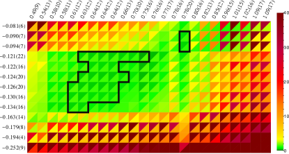
Figure 2: For each combination of parameterizations of $S0$ (columns) and $S2$ (rows), each ordered by the magnitude of their scattering length in $m^{-1}_{\pi}$ units, the box is colored according to the average value of $d^{2}/N_{\mathrm{smpl}}$ (upper triangle) and $\tilde{\chi}^{2}/N_{\mathrm{lat}}$ (lower triangle) over $S0$, $P1$, $S2$. The region indicated by the black outline shows parameterization combinations that have all amplitudes having metric values below the cutoffs presented in the text.

The acceptable dispersed amplitudes, $\tilde{t}^{I}_{\ell}(s)$, have several desirable properties, owing to the fact that they effectively respect unitarity, analyticity and crossing symmetry to the greatest extent possible. Firstly, the sub-threshold behavior of the amplitudes, which was previously essentially unconstrained by data, and which showed significant deviation between parameterization choices, now becomes consistent, and divergence-free down to the opening of the left-hand cut.

The location of the $\rho$ resonance pole in the dispersed $P1$ amplitudes is found to be entirely compatible with the small spread observed in the input lattice amplitudes, as expected for a narrow resonance. On the other hand, for the $\sigma$ pole in $S0$, which at $m_{\pi}\sim 239$ MeV is lying deep in the complex plane, the acceptable dispersed amplitudes all have a pole that lies in a much-reduced region, as shown in Figure 3. As hoped, the imposition of crossing symmetry, constrained by lattice data in all relevant isospins and low partial-waves, has led to a robust extraction of the $\sigma$ pole position, independent of any significant parameterization dependence.

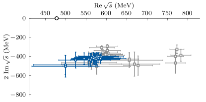
Figure 3: $m_{\pi}\sim 239$ MeV $\sigma$ pole location for lattice-fit amplitudes (gray) and dispersed amplitudes satisfying the metric cuts described in the text (blue).

In the $m_{\pi}\sim 283$ MeV case, the $S0$ lattice amplitudes indicated that the $\sigma$ could be either a virtual bound-state or a subthreshold resonance, depending upon parameterization choice, with a spread in pole positions. Those dispersed amplitudes that meet the metric cuts show a reduced scatter in pole location, but a definitive statement about whether the state is a virtual bound-state, or a subthreshold resonance at this pion mass cannot yet be made.

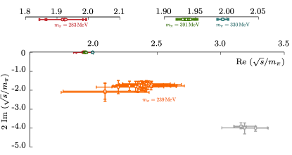
Figure 4: $\sigma$ pole evolution with changing light-quark mass corresponding to $m_{\pi}=$ 391 MeV (green, bound-state, non-dispersive), 330 MeV (blue, bound-state, non-dispersive), 283 MeV (red, virtual bound-state, dispersive), 239 MeV (orange, resonance, dispersive). Gray points correspond to the dispersive extractions from experimental data given in Refs. [4, 5, 6]. The top part of the plot represents two different insets of the real axis around the two-pion threshold.

Taking the $\sigma$ pole results from dispersive analysis at $m_{\pi}\sim 239,\,283$ MeV and supplementing them with two heavier quark masses where the dispersive analysis is not required as the $\sigma$ is a well-determined near-threshold bound-state, we show in Figure 4 the quark mass evolution of the $\sigma$ pole. In distinction to the $\rho$, which exhibits a simple quark-mass dependence corresponding to an approximately constant coupling to $\pi\pi$ [29], compatible with previous expectations [34, 35], the $\sigma$ undergoes a dramatic rapid transition from bound to resonant state, appearing to pass through a virtual bound-state stage in a narrow region of pion mass.

Summary — We have presented a dispersive approach to analyze elastic hadron-hadron scattering information provided by lattice QCD, applied here to the $\pi\pi$ case. We have observed that the sensitivity of $S$–wave scattering lengths and broad resonance pole locations to choice of parameterization form can be largely eliminated, indicating that reliable results can be extracted from lattice QCD calculations without the need to enforce amplitude features not motivated by the lattice data, such as subthreshold amplitude zeroes at fixed locations. The well-constrained amplitudes obtained in this study can be used in future lattice QCD calculations in which the $\pi\pi$ $S$-wave scattering system is coupled to external currents [36, 37, 38, 39], where well-defined form-factors of resonances can be extracted from pole residues, providing structural information that will aid in the determination of the compositeness of the $\sigma$ as the light quark mass is varied.

Supplemental material

• Dispersion Relations

• High-Energy Parameterization

• Dispersed Amplitude Metrics

• Dispersed Amplitudes below threshold

• Minimally subtracted dispersion relations

• $m_{\pi}=239\,\mathrm{MeV}$ $I=2$ amplitudes

• Applying dispersion relations to $m_{\pi}=283\,\mathrm{MeV}$ amplitudes

I Dispersion Relations

Ref. [33] presents the derivation of the twice-subtracted dispersion relations, commonly referred to as “Roy equations”, that we have used in this letter. The particular choice of subtractions made in this derivation are such that the functions $\tau^{I}_{\ell}(s)$ in

$$\tilde{t}^{I}_{\ell}(s)=\tau^{I}_{\ell}(s)+\sum_{I^{\prime},\ell^{\prime}}\int_{4m_{\pi}^{2}}^{\infty}\!\!\!ds^{\prime}\,K^{II^{\prime}}_{\ell\ell^{\prime}}\!(s^{\prime}\!,s)\;\mathrm{Im}\,t^{I^{\prime}}_{\ell^{\prime}}(s^{\prime})\,,$$ (4)

take the form

$$\tau^{0}_{0}(s)/m_{\pi} =\tfrac{1}{3}\big{(}a^{0}_{0}+5a^{2}_{0}\big{)}+\tfrac{1}{3}\big{(}2a^{0}_{0}-5a^{2}_{0}\big{)}\frac{s}{4m_{\pi}^{2}}\,,$$

$$\tau^{1}_{1}(s)/m_{\pi} =\tfrac{1}{18}\big{(}2a_{0}^{0}-5a^{2}_{0}\big{)}\frac{s-4m_{\pi}^{2}}{4m_{\pi}^{2}}\,,$$

$$\tau^{2}_{0}(s)/m_{\pi} =\tfrac{1}{6}\big{(}2a^{0}_{0}+a^{2}_{0}\big{)}-\tfrac{1}{6}\big{(}2a^{0}_{0}-5a^{2}_{0}\big{)}\frac{s}{4m_{\pi}^{2}}\,,$$ (5)

where the $S$-wave scattering-lengths, $a^{I}_{0}\equiv\mathrm{Re}\,t^{I}_{0}(s=4m_{\pi}^{2})/m_{\pi}$, are parameters that we fixed using the amplitudes fitted to data in $I=0,2$. The contribution of the integrals goes to zero as $\sqrt{s}\to 2m_{\pi}$.

Figure 5 illustrates the dispersive kernel functions relevant for obtaining the $S0$ dispersed amplitude, $K^{0I^{\prime}}_{0\ell^{\prime}}\!(s^{\prime}\!,s)$, where we observe that crossed-channels will have an influence at elastic scattering energies, and that all contributions from amplitudes at high energies are heavily suppressed due to the subtraction scheme. The right column shows the kernels evaluated at complex values of $s$ where we observe the pole singularity at real $s^{\prime}=s$ being smoothed out. The lowest entry in the right column is evaluated in the region where the $\sigma$ pole is eventually found for $m_{\pi}\sim 239\,\mathrm{MeV}$, and here we observe that the influence of the crossed-channels, $P1$ and $S2$ (which contribute to the left-hand cut), will be significant.

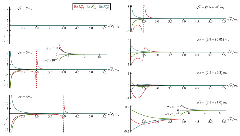
Figure 5: Real part of kernel functions in Eq. 4 contributing to dispersion of $S0$, $\mathrm{Re}\,K^{0I^{\prime}}_{0\ell^{\prime}}$, plotted in units where $1$ on the $y$-axis represents a value $4m_{\pi}^{2}$. Left column: functions evaluated on the real $s^{\prime}$–axis for three values of $s$ – inset indicates the behavior in the high-energy region. Right column: Kernel functions evaluated for complex values of $s$.

In our implementation of Eq. 4, we divide the integration from threshold to infinity into two parts: an integration from threshold to $s_{h}$ in which the input $\mathrm{Im}\,t^{I^{\prime}}_{\ell^{\prime}}(s^{\prime})$ comes from fits to lattice QCD computed finite-volume spectra, and then an integration from $s_{h}$ to infinity where the total amplitude, defined as

$$T^{I}(s,t,u)=32\pi\sum_{\ell}(2\ell+1)\,t^{I}_{\ell}(s)\,P_{\ell}(\cos\theta_{s}),$$ (6)

is given by a parameterization of the Regge form that we will describe in the next section. For both cases $m_{\pi}\sim 239,\,283$ MeV, we use $\sqrt{s_{h}}=0.22\,a_{t}^{-1}$, which for $m_{\pi}\sim 239$ MeV corresponds to $5.6\,m_{\pi}=1.34\,\mathrm{GeV}$. The lattice inputs are described by using previous parameterizations already presented in [19], or parameterizations similar to those described in Section III of [29]. They are constrained as follows:

• $\mathbf{S2,D2}$: these amplitudes, whose spectra are compatible with there being no inelasticity, are constrained by fitting energy levels up to around $a_{t}E_{\mathsf{cm}}=0.22$ for both $m_{\pi}\sim 239,\,283$ MeV masses.

• $\mathbf{P1}$: this amplitude is constrained by fitting energy levels up to around $a_{t}E_{\mathsf{cm}}=0.185(0.19)$ for $m_{\pi}\sim 239(283)$ MeV, slightly above the $K\bar{K}$ threshold. As presented in Ref. [27], there is negligible inelasticity up to $0.22$, and as such, we use the extrapolation of the elastic amplitude up to $s_{h}$. In fact, because the phase-shift in this region is very close to $180^{\circ}$, the imaginary part that enters the dispersion relations is anyway very close to zero.

• $\mathbf{S0}$: this amplitude is constrained by fitting energy levels up to around $a_{t}E_{\mathsf{cm}}=0.1585(0.16)$ for $m_{\pi}\sim 239(283)$ MeV, slightly below the $K\bar{K}$ threshold. The presence of a scalar resonance analogous to the $f_{0}(980)$ can cause the $K\bar{K}$ amplitude to turn on rapidly, and we have not yet attempted coupled-channel descriptions in this region, where $4\pi$ channels may also be relevant. In practice, we use extrapolations of the elastic amplitude up to $s_{h}$, and for different parameterizations, these extrapolations differ significantly. However, as observed in Figure 2 in the Letter, the main variation in the dispersion relation metrics comes from the behavior of the amplitudes at threshold (characterized by the scattering length), so it appears that there is little sensitivity to this extrapolation region, suppressed as it is by the rapidly decreasing dispersion relation kernels.

The dispersive relations, Eq. 1 in the Letter, are evaluated for $m_{\pi}\sim 239$ MeV at 100 evenly spaced energy values in the range, $a_{t}\sqrt{s}\in[0.074,0.14]$, and interpolation is used between these points.

The input lattice amplitudes carry statistical uncertainties associated with being constrained by energy levels computed on a finite ensemble of lattice gauge configurations. These are available in the form of (correlated) statistical uncertainties on the parameters of each amplitude parameterization. In addition, as discussed in the next section, the high-energy Regge parameterized amplitudes carry an assigned conservative uncertainty. Given a set of fits to lattice data with parameters $\{a_{i}\}$, and Regge contributions with a fixed fractional uncertainty, the dispersion relation uncertainties $\Delta\tilde{f}^{I}_{\ell}(s,\{a_{i}\})$ are obtained by linearized (correlated) error propagation at each sampled energy point. The error bands in Figure 1 in the Letter show this quantity. For the evaluation of the metric $d^{2}$, the error is calculated for the difference $\big{[}\tilde{f}^{I}_{\ell}(s)-f^{I}_{\ell}(s)\big{]}(\{a_{i}\})$ between the input amplitude and the dispersed amplitude.

In this work, we have studied two pion masses for which the $\sigma$ appears as a pole in the unphysical Riemann sheet, while at higher pion masses we observe a transition to the $\sigma$ being a bound-state pole on the physical Riemann sheet. The dispersion relations can be modified for this case of a stable $\sigma$, where the isoscalar amplitude $T^{0}(s,t,u)$ will have two poles in addition to the right- and left-hand cuts. These poles come from the $\sigma$ propagator appearing in the $s$– and $u$–channels. In this approach, the values of the position and residue of these poles should be considered as “fixed input” to the dispersion relations, to be provided by parameterizations fitted to the lattice spectra. The $s$–channel $\sigma$ pole remains a pole when the amplitude is projected into the $s$–channel $S$–wave, while the $u$–channel $\sigma$ pole generates a cut that is present in all partial-waves. In practice, for a $\sigma$ bound-state pole very close to physical scattering, the pole position and residue, and the $S$–wave scattering length can be determined from the lattice data with low systematic uncertainty, reducing the need to consider a dispersive approach.

As this Letter was in the final stages of production, Ref. [30] appeared, presenting an implementation of the above case where a bound-state $\sigma$ is present. This preprint reported on the use of Hadron Spectrum Collaboration results at $m_{\pi}\sim 391$ MeV, where lattice data is available in the inelastic region, choosing to obtain a dispersive solution by setting several matching conditions at $\sqrt{s_{m}}=1098$ MeV and fixing the energy at which the $P1$ wave crosses $90^{\degree}$. Their solution, continued into the complex energy plane, yielded, as well as the stable $\sigma$, also resonance poles compatible with the $f_{0}(980)$–like state reported in the coupled-channel analysis, Ref. [28].

Our approach, applied here at lower values of the quark mass where the $\sigma$ is unbound, differs from that in Ref. [30] in that we do not solve dispersion relation by setting matching conditions at single points in energy, but rather by selecting those amplitude parameterizations which acceptably respect fundamental constraints as measured by the metrics defined below. Both approaches are extensions of successful two-body dispersive analyses implemented at the physical quark mass [47, 48, 49, 4, 50, 32, 51, 52, 5, 6, 22, 53, 54, 55].

Ref. [32] provides a derivation of minimally subtracted dispersion relations, in which only those subtractions needed for convergence are implemented, often referred to as “GKPY equations”. We will present results using these equations in Section V below.

II High-energy parameterization

Generally, it is observed that scattering amplitudes at high energy cease to show features of individual resonances, becoming smooth functions of energy. In the limit $s\gg t$, the complex angular momentum, or “Regge” approach proves to be an efficient method to parameterize scattering amplitudes in terms of a modest number of parameters describing $t$–channel Regge trajectories and their residues [56, 57, 58]. This approach has been used extensively to describe experimental scattering data, with good descriptions of $\pi\pi$ scattering at high energy being obtained by inclusion of Pomeron, $\rho$ and $f_{2}$ trajectories [59, 32, 51].

For the current analysis at unphysical values of the light quark mass, we lack any high-energy scattering data with which to constrain a Regge parameterization, but we can use the relationship between Regge trajectories and resonance states exchangeable in the $t$–channel to infer the required quark-mass scaling. In particular, we will use an average of the parameterizations given in [32, 51] (specifically we use the “CFD” results from Ref. [32]), adapted to our pion masses in a simplistic approach.

The Pomeron trajectory is typically associated with gluonic exchanges, and as such we will assume that the parameters obtained from fits to physical data can be used without adjustment for the changed light quark mass. On the other hand, the $\rho$ trajectory includes the $\rho$ resonance, and the residue of this trajectory in $\pi\pi$ scattering can be related to the decay width for $\rho\to\pi\pi$, which does change with varying light quark mass. We keep the Regge trajectory $\alpha_{\rho}(s)$ fixed at the physical value, and only adjust the residue for the changed quark mass. Equation (E.5) from Ref. [47],

$$\Gamma_{\rho}=\frac{\lambda}{96\pi M_{\rho}^{2}}\left(M_{\rho}^{2}-4M_{\pi}^{2}\right)^{\frac{3}{2}},$$ (7)

indicates how to scale the residue (which is proportional to $\lambda$) given the $M_{\rho},\Gamma_{\rho}$ computed in lattice QCD at an unphysical light quark mass. For $m_{\pi}\sim 239$ MeV we take $M_{\rho}=793.7$ MeV and $\Gamma_{\rho}=91.2$ MeV, while for $m_{\pi}\sim 283$ MeV we use $M_{\rho}=798.8$ MeV and $\Gamma_{\rho}=60.6$ MeV. The residue, $\beta$, present for $\rho$ exchange, given in Ref. [32, 51], is scaled by the ratio of the lattice $\lambda$ to the physical value, which we take as $\lambda_{\mathrm{phys}}=72$. The $\rho$–computed ratio is also used (as a crude first approximation) to scale the $f_{2}$ residue.

The Regge implementations of Refs [32, 51], with the quark-mass scaled residues, are used to calculate the $\pi\pi$ cross-sections in the $s$-channel, according to

$$\sigma^{I_{s}}(s)=\frac{\mathrm{Im}\,T^{I_{s}}(s,0)}{\sqrt{s(s-4m_{\pi}^{2})}}.$$ (8)

Figure 6 shows these for the $m_{\pi}\sim 239$ MeV case, along with the average of the two parameterizations, with a conservatively assigned $30\%$ error which we propagate through our current analysis.

These amplitudes are used in the dispersion relations from $s_{h}$ up to infinity, but note that their contributions are heavily suppressed by the kernels, which as shown in the previous section, fall rapidly with increasing energy. In Figure 7, we present the contribution of the high-energy parameterized amplitude to the dispersed amplitudes in the elastic scattering region. We define

$$\tilde{f}^{I}_{\ell}(s)\big{|}_{\mathrm{Regge}}\equiv\sum_{I^{\prime},\ell^{\prime}}\int_{s_{h}}^{\infty}\!\!ds^{\prime}\;\mathrm{Re}\,K^{II^{\prime}}_{\ell\ell^{\prime}}(s^{\prime},s)\;\mathrm{Im}\,t^{I^{\prime}}_{\ell^{\prime}}(s^{\prime})\big{|}_{\mathrm{Regge}}\,,$$ (9)

and compare this to the total dispersed amplitude, which is dominated by the amplitudes constrained by lattice QCD data for $s<s_{h}$. The plotted ratio between the high-energy contribution and the relative uncertainty, $\Delta\big{[}\tilde{f}^{I}_{\ell}(s)-f^{I}_{\ell}(s)\big{]}$, indicates that the results of the analysis presented in the Letter are not sensitive to the detailed modeling of the Regge amplitudes.

Figure 6: Regge contributions to $\sigma^{I_{s}=0}(s)$ (left), $\sigma^{I_{s}=1}(s)$ (center) and $\sigma^{I_{s}=2}(s)$ (right) for $m_{\pi}\sim 239$ MeV. Parameterizations taken from Ref. [32] (blue) and Ref. [51] (orange), scaled to be applicable to the current pion mass. In our dispersive analysis, we use the average of the two (gray) assigning a conservative 30% fractional uncertainty.

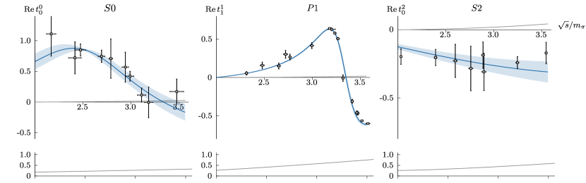
Figure 7: Top row: Blue curves show the real part of the $S0$, $P1$, $S2$ partial-wave amplitudes for $m_{\pi}\sim 239$ MeV (amplitude combination indicated by the black star in Figure 9). The gray curves lying close to zero in each case show the contribution to the amplitude, $\tilde{f}^{I}_{\ell}(s)\big{|}_{\mathrm{Regge}}$, coming from the high-energy amplitude parameterization (as defined in Eq. 9).
Bottom row: Ratio of $\tilde{f}^{I}_{\ell}(s)\big{|}_{\mathrm{Regge}}$ and the denominator in the parenthesis of Eq. 10, indicating the high-energy contribution in units of the relative uncertainty at each energy.

III Dispersed amplitude metrics

As discussed in the Letter, we retain only those dispersed amplitudes which are both compatible with unitarity, determined by having real part in agreement with the input amplitude (which itself was exactly unitarity preserving), and which provide a reasonable description of the original lattice data. These criteria are assessed using two numerical metrics.

A metric which compares the real part of the dispersed amplitude, $\tilde{f}^{I}_{\ell}(s)\equiv\mathrm{Re}\,\tilde{t}^{I}_{\ell}(s)$, to the real part of the input amplitude, $f^{I}_{\ell}(s)\equiv\mathrm{Re}\,t^{I}_{\ell}(s)$, in order to enforce unitarity, is

$$\big{[}d^{2}\big{]}^{I}_{\ell}\equiv\sum_{i=1}^{N_{\mathrm{smpl}}}\left(\frac{\tilde{f}^{I}_{\ell}(s_{i})-f^{I}_{\ell}(s_{i})}{\Delta\big{[}\tilde{f}^{I}_{\ell}(s_{i})-f^{I}_{\ell}(s_{i})\big{]}}\right)^{2}\,.$$ (10)

The sampling of points in the sum runs from just above the $\pi\pi$ threshold, $a_{t}\sqrt{s}=0.0836$, to $a_{t}\sqrt{s}=0.14$. Excluding the lowest 30 MeV above threshold reduces the sensitivity to high-order derivatives of the scattering amplitude at threshold, a sensitivity that is peculiar to this particular difference. In practice, we use 85 points to evaluate this metric. The uncertainty on the difference at each energy sample (appearing in the denominator) is calculated by linear propagation of the (correlated) amplitude parameter uncertainties and the (uncorrelated) high-energy Regge model uncertainty.

In order to compare the dispersed amplitudes directly to the ‘lattice amplitude data’, we use a $\chi^{2}$-like construction which accounts for both the correlation between different lattice data points and the correlation between the amplitude uncertainty and the energy uncertainty of each point,

$$\big{[}\tilde{\chi}^{2}\big{]}^{I}_{\ell} \equiv\sum_{i,j=1}^{N_{\mathrm{lat}}}\left(\tfrac{\mathfrak{f}_{i}-\tilde{f}^{I}_{\ell}(s_{i})}{\Delta_{i}}\right)\mathrm{corr}(\mathfrak{f}_{i},\mathfrak{f}_{j})\left(\tfrac{\mathfrak{f}_{j}-\tilde{f}^{I}_{\ell}(s_{j})}{\Delta_{j}}\right)\,,$$

$$\Delta_{i}^{2} =\big{(}\Delta\mathfrak{f}_{i}\,\,\,\frac{d\tilde{f}^{I}_{\ell}(s_{i})}{dE_{i}}\Delta E_{i}\big{)}\begin{pmatrix}1&-c_{i}\\ -c_{i}&1\end{pmatrix}\begin{pmatrix}\Delta\mathfrak{f}_{i}\\ \frac{d\tilde{f}^{I}_{\ell}(s_{i})}{dE_{i}}\Delta E_{i}\end{pmatrix},$$ (11)

where $E_{i}=\sqrt{s_{i}}$ is the “$x$” variable for which $\mathfrak{f}_{i}$ is calculated. In the second expression, the “$x,y$” correlation, $c_{i}$, for points obtained from Lüscher finite-volume analysis is typically $\pm 1$, and in Figure 8 we present a geometric illustration of the construction of the effective uncertainty, compatible with the equation above, for the case $c_{i}=-1$. $\Delta^{2}_{i}$ is considered as an “effective variance weight”; explicit examples with and without correlations between the $x$ and $y$ values, and a justification of the formula above are given in [60, 61]. The values of $c_{i}$ and $\mathrm{corr}(\mathfrak{f}_{i},\mathfrak{f}_{j})$ are obtained from the original lattice ensemble distributions.

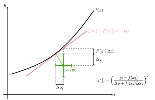
Figure 8: Geometric illustration of the construction of a linearized $\chi^{2}$ contribution for a data-point having $x,y$ correlation of $-1$. The data-point shown will contribute $1$ to the $\chi^{2}$ in agreement with the apparent $1\sigma$ deviation from the curve along the diagonal direction.

Applying these metrics to the amplitudes obtained from the dispersion relations generates Figure 2 in the Letter. In the Letter we apply cuts $d^{2}/N_{\mathrm{smpl}}<1$ and $\tilde{\chi}^{2}/N_{\mathrm{lat}}<2$, retaining only those amplitudes which satisfy these for all partial-waves, $S0,P1,S2$. In Figure 9, we show the effect of relaxing these cuts somewhat. The four superimposed boundaries correspond to:

• white: all amplitude combinations with all $d^{2}/N_{\mathrm{smpl}}<3$ and $\tilde{\chi}^{2}/N_{\mathrm{lat}}<3$

• gray: all amplitude combinations with all $d^{2}/N_{\mathrm{smpl}}<1$ and $\tilde{\chi}^{2}/N_{\mathrm{lat}}<3$

• dark gray: all amplitude combinations with all $d^{2}/N_{\mathrm{smpl}}<2$ and $\tilde{\chi}^{2}/N_{\mathrm{lat}}<2$

• black: all amplitude combinations with all $d^{2}/N_{\mathrm{smpl}}<1$ and $\tilde{\chi}^{2}/N_{\mathrm{lat}}<2$

Figure 9 indicates that somewhat looser cuts can slightly increase the range of acceptable scattering length values, but as shown in Figure 10 (for the sample points indicated by the white and gray stars in Figure 9), they do so by allowing increasing departures from unitarity, or from an acceptable description of the lattice data.

Nevertheless, if one allows these looser cuts, we note that the $\sigma$ pole location remains within the region established by the tighter cuts, as shown in Figure 11, indicating that our particular choice of metric cuts is not introducing a significant systematic error.

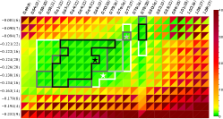
Figure 9: For each combination of parameterizations of $S0$ (columns) and $S2$ (rows), each ordered by the magnitude of their scattering length, the box is colored according to the average value of $d^{2}/N_{\mathrm{smpl}}$ (upper triangle) and $\tilde{\chi}^{2}/N_{\mathrm{lat}}$ (lower triangle) over $S0$, $P1$, $S2$. The different regions indicated by the color contours show the parameterization combinations respecting the cuts described in the text. Three example parameterization combinations are indicated by black, gray, and white stars, which are used for illustration in other figures.

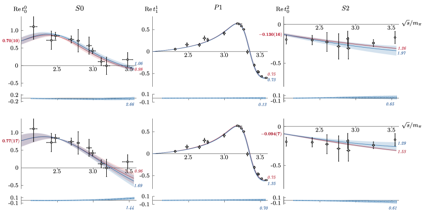
Figure 10: Real parts of $S0$, $P1$, $S2$ partial-wave amplitudes for $m_{\pi}\sim 239$ MeV, for input (red) and dispersed output (blue). Amplitude combinations correspond to the stars in Figure 9: white (upper panel), gray (lower panel). The colored numbers with an error estimate represent the different scalar scattering lengths. The red italic numbers represent the $\tilde{\chi}^{2}/N_{\text{lat}}$ values for the fits to the data, whereas the blue numbers on those same panels represent the dispersive $\tilde{\chi}^{2}/N_{\text{lat}}$ value. Beneath each panel, values of the quantity in the large parentheses in Eq. 10 at $N_{\mathrm{smpl}}=85$ points are given, and the numbers listed there represent the $d^{2}/N_{\text{smpl}}$ values.

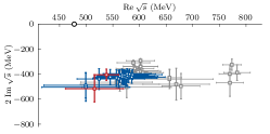
Figure 11: $S0$ pole locations for lattice-fit amplitudes (gray), dispersed amplitudes satisfying the tighter metric cuts described in the text (blue), and for the two sample points (white and gray stars in Figure 9) satisfying looser cuts (red).

IV Dispersed amplitudes below threshold

The amplitude parameterizations used to describe lattice QCD spectra above threshold (and sometimes slightly below threshold) in a particular partial-wave are built to exactly obey unitarity above threshold, but they are not typically guaranteed to be free of unphysical behavior far below threshold. Usually this is excused as irrelevant since the amplitudes are only needed in a small region around the real energy axis above threshold (for example when narrow resonances are sought), but if extrapolation further into the complex energy plane is required, such parameterization artifacts may be problematic.

The use of dispersion relations can remedy this problem. Since the dispersion relations take as input the amplitudes only above threshold (where they are well constrained), while the subthreshold behavior is controlled by the kernel functions (which have correct analytic properties), the behavior of the dispersed amplitudes below threshold is rendered free of singularities.

This is illustrated in Figure 12, where the $S0$ and $S2$ amplitudes are shown for $m_{\pi}\sim 239$ MeV. The upper panel in each case shows the input lattice amplitudes (where amplitudes that systematically fail the metric cuts are shown in red) where subthreshold divergences are observed to be present, as is a significant scatter of behavior such that one can argue that the lattice data (above threshold, in a single partial-wave) has not constrained in any reliable way the amplitude behavior far below threshold. On the other hand, in the lower panel, we observe that all dispersed amplitudes satisfying the metric cuts show broadly compatible singularity-free behavior below threshold. The scatter of behaviors of acceptable amplitudes is observed to be at the level of the uncertainty (shown for one example amplitude by the gray band).

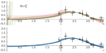
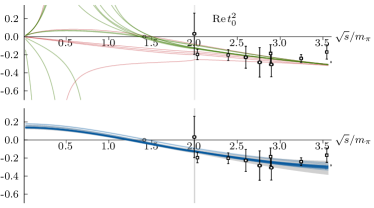
Figure 12: Top panels: Central values of the $m_{\pi}\sim 239$ MeV S0 and S2 real parts, both above and below the two-pion threshold, for all amplitude parameterizations. Those plotted in green correspond to parameterizations that produce at least one combination respecting the metric cuts presented in the Letter, while all others are plotted in red. Open circles on axis indicate the locations of Adler zeroes in the leading-order of $\chi$PT.
Bottom panels: Dispersive real parts for all amplitude combinations respecting the metric cuts presented in the Letter. The uncertainty on one example amplitude is shown by the gray band.

In Figure 12, both sets of dispersed amplitudes are observed to feature a zero-crossing below threshold, located near to $s/m_{\pi}^{2}\approx 0.8$ for $S0$ and $s/m_{\pi}^{2}\approx 1.6$ for $S2$. The presence of such zeroes, known as “Adler zeroes”, is an expectation of chiral perturbation theory [63], and we show in the figure the expected location at leading order ($s/m_{\pi}^{2}\approx\tfrac{1}{2}$ for $S0$ and $s/m_{\pi}^{2}\approx 2$ for $S2$). The zeroes in the dispersed amplitudes are observed to differ from these expectations, with a non-negligible spread, and hence we suggest that analyses of lattice QCD obtained spectra using amplitudes which enforce an Adler zero fixed at the leading order location are potentially introducing a systematic bias which may impact results such as scattering lengths or $\sigma$ pole positions.

In Section VII we will present comparable results for the case where $m_{\pi}\sim 283$ MeV, only slightly further from the chiral limit, noting that in the case of the $S0$ amplitude, it is no longer clear that an Adler zero is even present in the dispersed amplitudes between the left-hand cut and the $\pi\pi$ threshold.

V Minimally subtracted dispersion relations

Minimally-subtracted dispersion relations, often referred to as GKPY equations, are constructed making only those subtractions required to get convergence, namely one subtraction for $I=0,2$ amplitudes and no subtractions for the $I=1$ amplitude [32]. The smaller number of subtractions means the high-energy contributions to the dispersion relations are not as strongly suppressed, with the kernel functions, in this case, falling off as $s^{-2}$ rather than $s^{-3}$ as was the case for twice-subtracted (Roy) dispersion relations. The subtraction functions in this case are just constants which, as before, depend only on the $S$-wave scattering lengths,

$$\tau^{0}_{0}(s)/m_{\pi} =\tfrac{1}{3}\big{(}a^{0}_{0}+5a^{2}_{0}\big{)}\,,$$

$$\tau^{1}_{1}(s)/m_{\pi} =\tfrac{1}{12}\big{(}2a_{0}^{0}-5a^{2}_{0}\big{)}\,,$$

$$\tau^{2}_{0}(s)/m_{\pi} =\tfrac{1}{6}\big{(}2a^{0}_{0}+a^{2}_{0}\big{)}\,.$$ (12)

In contrast to the twice-subtracted equations, the dispersive integrals do not go to zero as $\sqrt{s}\to 2m_{\pi}$, and their value in this limit must conspire with the $\tau$ values above to generate the correct threshold behavior. These minimally-subtracted equations have two main advantages over the twice-subtracted variant. Firstly, the error on the dispersed amplitudes grows less quickly with increasing energy above threshold, which in previous analyses led to lower uncertainties on resonance pole locations and residues [5]. Secondly, the scattering length values can be determined, rather than needing to be supplied as input. The primary disadvantage of minimally-subtracted equations is their sensitivity to the high-energy region of scattering, which in this lattice application we have relatively little constraint on. We will return to this later in this section.

In the left panel of Figure 13 we show the $d^{2}$ and $\tilde{\chi}^{2}$ metrics for the output of minimally-subtracted dispersion relations using the same lattice amplitude parameterizations as shown in Figure 2 in the Letter. The black boundary superimposed on the plot is the one selected according to the metric cuts applied to the twice-subtracted results, and we see that a large fraction of acceptable solutions of the minimally-subtracted dispersion relations also lie in this region.

In the right panel of Figure 13 we show a metric designed to show how well the Olsson sum rule [64],

$$\operatorname{Re}\tilde{T}^{I_{t}=1}(4m_{\pi}^{2},0) =\frac{4m_{\pi}^{2}}{\pi}\int_{4m_{\pi}^{2}}^{\infty}\!ds^{\prime}\,\frac{\operatorname{Im}T^{I_{t}=1}(s^{\prime},0)}{s^{\prime}\left(s^{\prime}-4m_{\pi}^{2}\right)},$$ (13)

is satisfied. In this expression, the $t$–channel definite isospin amplitude can be expressed in terms of the $s$–channel definite isospin amplitudes by $T^{I_{t}=1}(s,t)=\frac{1}{3}T^{0}(s,t)+\frac{1}{2}T^{1}(s,t)-\frac{5}{6}T^{2}(s,t)$, and these are expressed in terms of a sum over the partial-wave amplitudes. The $t$–channel amplitude at threshold is equal to a combination of the $S$–wave scattering lengths, $\operatorname{Re}\tilde{T}^{I_{t}=1}(4m_{\pi}^{2},0)=\tfrac{32\pi}{6}(2a^{0}_{0}-5a^{2}_{0})$, so the quantity plotted, $\left(\frac{\psi}{\Delta\psi}\right)^{2}$, where

$$\psi=2a_{0}^{0}-5a_{0}^{2}-\frac{6m_{\pi}}{8\pi^{2}}\int_{4m_{\pi}^{2}}^{\infty}\!ds^{\prime}\,\frac{\operatorname{Im}T^{I_{t}=1}(s^{\prime},0)}{s^{\prime}\left(s^{\prime}-4m_{\pi}^{2}\right)}\,,$$ (14)

should vanish if this dispersive sum rule is fulfilled.

Figure 14 shows an example of the dispersed amplitudes coming from minimally-subtracted dispersion relations compared to those from twice-subtracted dispersion relations for the same set of input lattice amplitude parameterizations, indicated by the black star in Fig. 9.

The amplitudes are observed to be compatible within errors over the entire energy region plotted, but if one examines the contribution to the minimally-subtracted amplitudes of the high-energy part of the input, one sees it is much larger than for the twice-subtracted variants. Measured as a fraction of the relative uncertainty $\Delta\big{[}\tilde{f}^{I}_{\ell}(s)-f^{I}_{\ell}(s)\big{]}$, depicted in the bottom row, it is seen to contribute at a level where one would worry about the correctness of the crudely-scaled Regge parameterization used. As such we do not consider these results to be model-independent consequences of the lattice QCD calculation. Nevertheless, the amplitude agreement with the twice-subtracted results inspires us to examine the $\sigma$ pole location, and as shown in Figure 15, we see that there is reasonable agreement with the twice-subtracted results with, as anticipated, smaller uncertainties on the pole location and the pole residue.

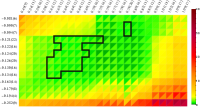
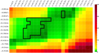
Figure 13: Left panel: Average values of $d^{2}/N_{\mathrm{smpl}}$ (upper triangle) and $\tilde{\chi}^{2}/N_{\mathrm{lat}}$ (lower triangle) for each pair of $S0$ (columns) and $S2$ (rows) parameterizations, computed using minimally-subtracted dispersion relations. The black outline indicates those amplitudes that passed the metric cuts in the twice-subtracted case.
Right panel: Values of $\left(\frac{\psi}{\Delta\psi}\right)^{2}$ as defined in the text, testing the degree to which the Olsson sum rule is satisfied.

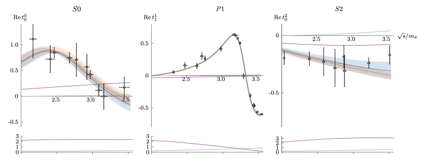
Figure 14: See Fig. 7 for comparison. Dispersed amplitudes produced by twice-subtracted (blue) and minimally-subtracted (orange) dispersion relations applied to input amplitudes indicated by the black star in Figure 9. Contributions to each from the high-energy parameterization is shown by the gray and purple curves, respectively. Bottom panels: Ratio of $\tilde{f}^{I}_{\ell}(s)\big{|}_{\mathrm{Regge}}$ and the denominator in the parenthesis of Eq. 10, indicating the high-energy contribution in units of the relative uncertainty at each energy, described by the same colors as before.

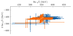
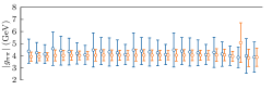
Figure 15: Left: $S0$ pole locations for twice-subtracted dispersed amplitudes satisfying the metric cuts described in the text (blue), and for the same amplitude combinations used in minimally-subtracted dispersion relations (orange).
Right: Corresponding couplings extracted from the pole residues.

VI $m_{\pi}\sim 239\,\mathrm{MeV}$ $I=2$ amplitudes

Ref. [19] and Ref. [27] reported on extractions of $I=0$ and $I=1$ finite-volume spectra from a $32^{3}\times 256$ anisotropic Clover lattice with light-quark masses such that $m_{\pi}\sim 239$ MeV. The corresponding spectra on this lattice with $I=2$ have not previously appeared in the literature, but have been computed for the purposes of this letter using the same techniques, range of energies, and similar operators to the ones reported in Ref. [29]. As observed in the previous work, the $D$-wave is very weak and repulsive, and can be described with one single parameter. The $S$-wave shows stronger repulsion, with phase-shift whose absolute value grows with the energy. Figure 16 shows discrete values of $S$ and $D$–wave phase-shifts determined from these spectra along with a sample of parameterizations. The parameterizations used here to describe the data correspond to a subsect of those types described in Section III of [29]. A compilation of the scattering lengths obtained from these fits was presented in Figure 5 of that work, and their explicit values, in $m^{-1}_{\pi}$ units, are given as part of Figure 1 in the Letter.

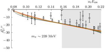
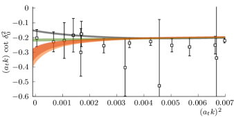
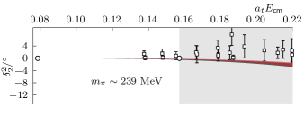
Figure 16: $I=2$ partial-wave amplitudes for $m_{\pi}\sim 239$ MeV. For $S$–wave (upper two panels), four example parameterizations are shown: a two-term conformal mapping (black), an effective range expansion with two terms (green), and two choices with an Adler zero fixed at the leading-order $\chi$PT location, a two-term conformal mapping (red), and an effective range expansion with two terms (orange). The $D$–wave phase-shift is shown in the lower panel illustrated with two parameterizations: a scattering length (red), and a conformal mapping with two terms (black).

VII Applying dispersion relations to $m_{\pi}\sim 283\,\mathrm{MeV}$ amplitudes

Ref. [29] presented another pion mass, $m_{\pi}\sim 283$ MeV for which the $\sigma$ appears to be unbound. Describing the lattice spectra with a range of parameterizations led to a spread of pole locations on the unphysical Riemann sheet, some of which were on the real axis and correspond to a virtual bound state while others had an interpretation as a subthreshold resonance as they lie off the real axis. The corresponding isoscalar scattering length, $a^{0}_{0}$ was determined to be relatively large and positive, while the isotensor $a^{2}_{0}$ changed relatively little compared to the $m_{\pi}\sim 239$ MeV case.

By virtue of Eqs. 4 and 5, both $a^{0}_{0}$ and $t^{0}_{0}(s>4m_{\pi}^{2})$ contribute to every partial wave in the dispersive analysis. In a limit where $a^{0}_{0}$ goes to infinity, the dispersed contribution coming from integrating $K^{I0}_{\ell 0}(s^{\prime}\!,s)\;\mathrm{Im}\,t^{0}_{0}(s^{\prime})$ must cancel this to ensure finite values of other partial waves, $t^{I}_{\ell}(s)$, at and above threshold. With twice-subtracted dispersion relations, this cancellation is particularly sensitive to amplitude behavior in the threshold region. We expect to find that only those amplitude parameterizations which “fine-tune” this cancellation will give rise to acceptable metric values. Figure 17 shows the relevant metric values for twice-subtracted dispersion relations computed for using the range of amplitude parameterizations found capable of describing the lattice QCD spectra in Ref. [29]. Applying the cuts $d^{2}/N_{\mathrm{smpl}}<1$ and $\tilde{\chi}^{2}/N_{\mathrm{lat}}<2$ to the twice-subtracted case leads to the very restricted set indicated by the black border. Examples of amplitudes which do and do not satisfy the metric cuts are given in Figure 18.

Figure 19 shows the relevant metric values for minimally-subtracted dispersion relations (left) and the Olsson sum-rule (right), with the boundary taken from Figure 17 superimposed. It is clear that the reduced sensitivity to the threshold region in these dispersion relations leads to far less of a restriction in the set of acceptable amplitudes. There is also less agreement between the twice- and minimally-subtracted dispersion relations for this pion mass.

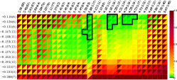
Figure 17: As Figure 1 in the Letter, but for the $m_{\pi}\sim 283$ MeV pion mass). For each combination of parameterizations of $S0$ (columns) and $S2$ (rows) the box is colored according to the average value of $d^{2}/N_{\mathrm{smpl}}$ (upper triangle) and $\tilde{\chi}^{2}/N_{\mathrm{lat}}$ (lower triangle) over $S0$, $P1$, $S2$. The region indicated by the black outline shows parameterization combinations that have all amplitudes having metric values below the cutoffs presented in the Letter.

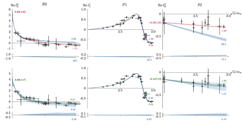
Figure 18: Real parts of $S0$, $P1$, $S2$ partial-wave amplitudes for $m_{\pi}\sim 283$ MeV. Data-points indicate the constraint provided by discrete lattice QCD spectra. The upper row shows an example of parameterizations (red) which describe well the lattice data, but which generate dispersed amplitudes (blue) that are in poor agreement, leading to large values of $d^{2}$ and $\tilde{\chi}^{2}$. The lower row shows a case where the lattice amplitudes (green) prove to be in good agreement with the dispersed amplitudes. The colored numbers with an error estimate represent the different scalar scattering lengths. The red(green) italic numbers represent the $\tilde{\chi}^{2}/N_{\text{lat}}$ values for the fits to the data, whereas the blue numbers on those same panels represent the dispersive $\tilde{\chi}^{2}/N_{\text{lat}}$ value. Beneath each panel, values of the quantity in the large parentheses in Eq. 10 at $N_{\mathrm{smpl}}=72$ points are given, and the numbers listed there represent the $d^{2}/N_{\text{smpl}}$ values.

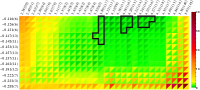
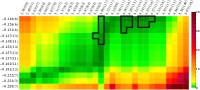
Figure 19: Minimally-subtracted dispersion relations applied to $m_{\pi}\sim 283$ MeV.
Left panel: Average values of $d^{2}/N_{\mathrm{smpl}}$ (upper triangle) and $\tilde{\chi}^{2}/N_{\mathrm{lat}}$ (lower triangle) for each pair of $S0$ (columns) and $S2$ (rows) parameterizations, computed using minimally-subtracted dispersion relations. The black outline indicates those amplitudes that passed the metric cuts in the twice-subtracted case.
Right panel: Values of $\left(\frac{\psi}{\Delta\psi}\right)^{2}$ as defined in the text, testing the degree to which the Olsson sum rule is satisfied.

Figure 20 shows the output dispersed amplitudes for twice-subtracted dispersion relations, retaining only those which satisfy the metric cuts. Comparing the input amplitudes to the dispersed, we observe that the spread in behavior at threshold in $t^{0}_{0}$ is reduced, and as expected all subthreshold singularities are removed. The $S2$ amplitude is seen to feature an Adler zero near $s/m_{\pi}^{2}\approx 2.3$, while the $S0$ amplitude does not appear to cross zero between the left-hand cut and threshold, in contradiction to the expectations of leading-order $\chi$PT.

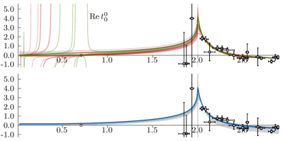
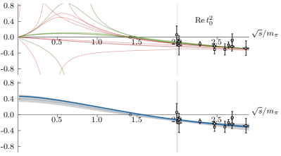
Figure 20: Top panels: Central values of the $m_{\pi}\sim 283$ MeV S0 and S2 real parts, both above and below the two-pion threshold, for all amplitude parameterizations. Those plotted in green correspond to parameterizations that produce at least one combination respecting the metric cuts presented in the Letter, while all others are plotted in red. Open circles on axis indicate the locations of Adler zeroes in the leading-order of $\chi$PT.
Bottom panels: Dispersive real parts for all amplitude combinations respecting the metric cuts presented in the Letter. The uncertainty on one example amplitude is shown by the gray band.

Finally, in Figure 21 we show the $\sigma$ pole locations extracted from those twice-subtracted dispersed amplitudes satisfying the metric cuts. The majority, but not all, of the accepted amplitudes feature a virtual bound-state pole. We focus on the virtual-bound state pole closer to threshold. As explained in [29], when the complex conjugate pole pair of a subthreshold resonances meet on the real axis below threshold the pole location’s dependence on the amplitude parameters develops an infinite slope. Near this point, the slopes are large, causing small uncertainties on the parameters to become large uncertainties on the pole location. We do not plot the pole locations for these noisy results but merely comment that they are compatible with the plotted virtual bound-state cases. Additionally, the couplings of these poles can become arbitrarily large, as two poles merge into one, similar to the behavior observed in Ref. [29]. Like in the previous case, the dispersive results produce larger statistical uncertainties but reduced systematic spread.

In unitarized versions of chiral perturbation theory [34, 20], the $\sigma$ is predicted to evolve from a sub-threshold resonance to a pair of virtual-bound states. When the pion mass is increased, one of these poles reaches the $\pi\pi$ threshold and becomes bound, while the other moves to lower energies as virtual-bound. As seen in this analysis, for this pion mass, no Adler zero is found on the real axis by the dispersion relations. In such a case, a third pole close to the left-hand cut is produced by some of our dispersive results. Unlike to the dispersive virtual-bound poles depicted in Fig. 21, the lighter poles suffer from large systematic scatter. Within the dispersive combinations that satisfy all metric cuts, they vary from being virtual-bound poles to a pair of resonances close to the left-hand cut. This behavior has also been observed in [30] for a $m_{\pi}\sim 391$ MeV pion mass, for which the heavier pole is actually bound on the physical sheet.

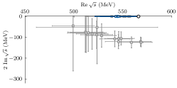
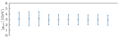
Figure 21: Left: $m_{\pi}\sim 283$ MeV $\sigma$ pole locations in $S0$ amplitude for lattice-fit amplitudes (gray) and dispersed amplitudes satisfying the metric cuts described in the text (blue).
Right: Coupling constants extracted from the pole residues.
Excluded from these plots are those cases in which poles feature very large uncertainties, including a case that describes a sub-threshold resonance.