Variational Bayes latent class approach for large real-world data

Abstract

[Summary]Bayesian approaches to clinical analyses for the purposes of patient phenotyping have been limited by the computational challenges associated with applying the Markov-Chain Monte-Carlo (MCMC) approach to large real-world data. Approximate Bayesian inference via optimization of the variational evidence lower bound, often called Variational Bayes (VB), has been successfully demonstrated for other applications. We investigate the performance and characteristics of currently available R and Python VB software for variational Bayesian Latent Class Analysis (LCA) of realistically large real-world observational data. We used a real-world data set, Optum^TM electronic health records, containing paediatric patients with risk indicators for Type 2 diabetes mellitus that is a rare form in paediatric patients. The aim of this work is to validate a Bayesian LCA patient phenotyping model for generality and extensibility and crucially to demonstrate that it can be applied to a realistically large real-world clinical data set. We find currently available automatic VB methods are very sensitive to initial starting conditions, model definition, algorithm hyperparameters and choice of gradient optimiser. The Bayesian LCA model was challenging to implement using the automatic VB method available but we achieved reasonable results with very good computational performance compared to MCMC.

, , and (2023), Variational Bayes latent class approach for EHR-based phenotyping with large real-world data, , .

1 Introduction

With growing acceptance by clinical regulators of using real-world evidence to supplement clinical trials, there is increasing interest in the use of Bayesian analysis for both experimental and observational clinical studies  ². The identification of specific patient groups sharing similar disease-related phenotypes is core to many clinical studies  ¹¹. Secondary use of electronic health records (EHR) data has long been incorporated in phenotypic studies  ¹⁴. Recent studies cover a wide range including health economic models  ²⁹, innovative trial designs for rare disease drug design  ⁴ and application of EHR information for antibiotic dose calculations  ¹. The most popular approach that has evolved for identification of cohorts belonging to a particular phenotype of interest is an expert-driven rules-based heuristic dependent on data availability for a given phenotypic study. Bayesian statistics provides a formal mathematical method for combining prior information with current information at the design stage, during the conduct of a study, and at the analysis stage.

Markov-Chain Monte-Carlo (MCMC) is considered the gold standard for Bayesian inference because it asymptotically converges to the true posterior distribution  ⁹. It’s application has been limited by the computational challenges of applying MCMC to large real-world clinical data. In Bayesian analysis, we are usually interested in the posterior distribution $p(Z|X)$ where $\mathbf{Z}$ are latent variables $\{z_{1},...,z_{n}\}$ and $\mathbf{X}$ are observed data $\{x_{1},...,x_{n}\}$. In many real-world models of interest the denominator of Bayes’ theorem, $p(X)$, often referred to as the evidence, can include latent variables that give rise to analytically or computationally intractable evidence  ²⁴. Approximate Bayesian inference via optimisation of the evidence lower bound is often called Variational Bayes (VB). In VB, optimization is used to find a tractable distribution $q(Z)$ from a family of distributions $\mathbf{Q}$ such that it is close to the posterior distribution $p(Z|X)$. The optimization aims to locate $q^{*}(Z)$, the distribution that minimise the Kullback-Leibler (KL) divergence of $q(Z)$ and $p(Z|X)$. This optimisation approach is often significantly more computationally efficient than MCMC at the expense of an estimated posterior.

VB has been successfully demonstrated for other patient phenotyping applications. Song et al. applied variational inference with a deep learning natural language processing (NLP) approach to patient phenotyping  ²⁵. Li et al. propose another NLP model, MixEHR, that applies a latent topic model to EHR data  ²¹. They apply a VB coordinate ascent approach to impute mixed disease memberships and latent disease topics that apply to a given patient EHR cohort. Hughes et al. developed a mean field VB model for multivariate generalized linear mixed models applied to longitudinal clinical studies  ¹⁶.

Latent Class Analysis (LCA) is widely used where we want to identify patient phenotypes or subgroups given multivariate data  ²⁰. A challenge in clinical LCA is the prevalence of mixed data, where we may have combinations of continuous, nominal, ordinal and count data together with missing data across variables. Bayesian approaches to LCA may better account for this data complexity. The Bayesian approach bridges rule-based phenotypes, which rely heavily on expert knowledge and opinion, and data-driven machine learning approaches, which are derived entirely from information contained in the data under investigation with no opportunity to apply relevant prior information. We consider the common clinical context where gold-standard phenotype information, such as genetic and laboratory data, is not available. A general model for this context has high potential applicability across disease areas and both primary and secondary clinical databases for use in clinical decision support. We used the same Bayesian LCA model form and motivating example as Hubbard et al.  ¹⁵, namely paediatric type 2 diabetes mellitus (T2DM), in order to test if the proposed LCA model translates to another electronic health records (EHR) database with the same target disease under study. Paediatric T2DM is rare so it naturally gives rise to the data quality issues we would like to explore with our approach. We extended the Hubbard et al. work to incorporate VB to investigate if a much larger EHR dataset is amenable to this form of Bayesian LCA model.

The application of VB in the context of phenotyping from EHR data using Bayesian LCA is a new application setting for variational inference of observational clinical data and one that potentially extends its scope to large real-world contexts. Our aim in this work is to investigate if a VB approach to Bayesian LCA phenotyping scales to realistically large EHR data and delivers a posterior approximation close to MCMC.

2 Data

This study used Optum^TM EHR data. This data set is comprised of EHR records from hospitals, hospital networks, general practice offices and specialist clinical providers across the United States of America. It includes anonymised patient demographics, hospitalizations, laboratory tests and results, in-patient and prescribed medications, procedures, observations and diagnoses. The data provides most information collected during a patient journey provided all care sites for a given patient are included in the list of Optum^TM data contributors. This data set is one of the most comprehensive EHR databases in the world  ²⁸ and is used extensively for real-world clinical studies  ⁶. The data set used Optum^TM EHR records between January 2010 and January 2020.

The initial processing step is to identify, from the overall Optum^TM dataset, a cohort of paediatric patients with elevated risk of T2DM, in order to subsequently perform phenotyping. For this analysis we extracted a patient cohort of paediatric patients with equivalent T2DM risk characteristics defined in Hubbard et al.  ¹⁵. The paediatric T2DM data structure was reproduced in order to test how well the proposed Bayesian LCA model translates from the Hubbard et al. PEDSnet EHR data to the Optum^TM EHR data. The PEDSnet data used in the Hubbard et al. work are located within the US Northeast region which comprises about 13% of the Optum^TM data. To account for potential variance of paediatric T2DM prevalence across the USA we used the Northeast subset of the Optum^TM EHR for the Bayes LCA comparison, although we also ran the study using all of the data. The data specification in Figure 1 shows how the data was extracted from Optum^TM EHR. The overall objective for this specification was to arrive at the same patient identification rules used by Hubbard et al. We also restricted the data variables to those used in the Hubbard et al. study. The patient BMI z-score was calculated from the US Centers for Disease Control and Prevention Growth Charts  ¹⁹ using patient age, sex and BMI. The full US Optum^TM EHR paediatric T2DM data extraction is compared with Hubbard et al. PEDSnet data in the supporting information (Table S1).

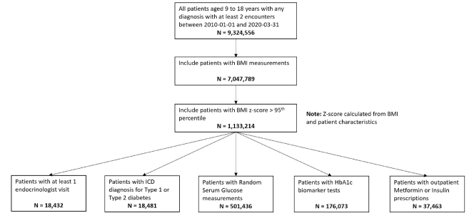
Figure 1: Data specification for paediatric patients at risk of T2DM in Optum^TM EHR database. The bottom row shows the number of patients having the specified study characteristics for the paediatric T2DM phenotype for the relevant variables.

3 Methods

Our aim is to investigate if a VB approach to Bayesian LCA phenotyping scales to realistically large EHR data and delivers a posterior approximation close to MCMC. We first reproduced the Hubbard et al. model  ¹⁵ with JAGS MCMC using the Optum^TM EHR T2DM data. This gives us confidence that the Bayes LCA model can generalise to other EHR data. We then followed up with the Stan  ⁵ implementations of Hamiltonian MCMC and VB to investigate how the model specification translates to other algorithmic approaches. We are particularly interested in how well the model scales to realistically large real-world clinical data, so we have focused on variational Bayes algorithms. As we could not find available closed-form implementations for variational Bayes LCA such as coordinate ascent or stochastic mean-field VB, we used Stan Automatic Differentiation Variational Inference (ADVI)  ¹⁷ for this study.

3.1 Bayes LCA Model

The canonical form for LCA assumes that each observation i, with observed J observed categorical response variables $x_{i}=\{x_{i1},x_{i2},…,x_{iJ}\}$, belongs to one of C latent classes. Class membership is represented by a latent class indicator $z_{i}=\{1,...,C\}$. The marginal response probabilities are

$$P(\textbf{x}_{i})=\sum\limits_{c=1}^{C}\pi_{c}\prod\limits_{j=1}^{J}P(x_{ij}|z_{i}=c)$$ (1)

Where $\textbf{x}_{i}$ is the response vector $(x_{i1},...,x_{iJ})^{T}$ for observation $i$ on J variables, $\textbf{z}_{i}$ is the latent class that observation $i$ belongs to and $\bm{\pi}_{c}$ is the probability of being in class $c$. The variables $x$ are assumed to be conditionally independent given class membership.

The Bayes LCA model applied is from Hubbard et al.  ¹⁵ and follows the general specification shown in Table 1. In the T2DM model example there are two classes in C (has T2DM or does not have T2DM) and three items with two categories each (2 biomarker indicators, 2 ICD disease codes and 2 diabetes medications). The latent phenotype variable for each patient, $D_{i}$, is assumed to be associated with patient characteristics that include demographics (for paediatric T2DM they are age, higher-risk ethnicity and BMI z-score) denoted by $X$ in the model specification, biomarker laboratory tests, clinical diagnostic codes and prescription medications. This model allows for any number of clinical codes or medications and in this model each clinical code and medication are binary indicator variables to specify if the code or medication was present for that patient. Since it is common for specific biomarker laboratory tests to be missing across a cohort of patients, the model includes an indicator variable per biomarker to indicate whether or not a specific biomarker data is available for that patient. Biomarker availability is an important component of the model since biomarkers are widely considered to be high quality prognostic data for many disease areas  ¹⁰ and availability of a biomarker measurement can be predictive of the phenotype as well as actual biomarker laboratory test result values since laboratory tests are often proxies for physician tentative diagnoses.

The model likelihood for the $i^{th}$ patient is given by

$$\mathcal{L}(\eta_{i},\beta^{D},\beta^{R},\beta^{Y},\beta^{W},\beta^{P},\tau^{2}|X_{i}) =\sum_{d=0,1}{P(D_{i}=d|\eta_{i},\beta^{D},X_{i})}$$

$$\prod_{j=1}^{J}{f(R_{ij}|D_{i}=d,X_{i},\beta_{j}^{R})f(Y_{ij}|D_{i}=d,X_{i},\beta_{j}^{Y},\tau_{j}^{2})^{R_{ij}}}$$

$$\prod_{k=1}^{K}{f(W_{ik}|D_{i}=d,X_{i},\beta_{k}^{W})}\prod_{l=1}^{L}{f(P_{il}|D_{i}=d,X_{i},\beta_{i}^{P})}$$ (2)

where $\beta^{D}$ associates the latent phenotype to patient characteristics, $\eta_{i}$ is a patient-specific random effect parameter and parameters $\beta^{R},\beta^{Y},\beta^{W}$ and $\beta^{P}$ associate the latent phenotype to patient characteristics and biomarker availability, biomarker values, clinical codes and medications respectively. $X_{i}$ represents $M$ patient covariates, such as demographics ($X_{i}=X_{i1},...,X_{i,M}$). The mean biomarker values are shifted by a regression quantity $\beta^{Y}_{j,M+1}$ for patients with the phenotypes compared to those without. Sensitivity and specificity of binary indicators for clinical codes, medications and presence of biomarkers are given by combinations of regression parameters. For instance, in a model with no patient covariates, sensitivity of the $k^{th}$ clinical code is given by $expit(\beta^{W}_{k_{0}}+\beta^{W}_{k_{1}})$, while specificity is given by $1-expit(\beta^{W}_{k_{0}})$, where $expit(\cdot)=exp(\cdot)/(1+exp(\cdot))$. We validated this model with a real-world example, namely paediatric T2DM. Table LABEL:table:modelExample indicates how the Bayes LCA phenotyping model maps to this disease area.

Informative priors are used to encode known information of the predictive accuracy of HbA1c and Glucose laboratory tests for T2DM. The biomarker priors inform a bimodal receiver operating characteristic (ROC) model since the biomarkers are normally distributed. The prior values were selected to correspond to an area under the ROC curve (AUC) of 0.95  ¹⁵.

Although the pediatric T2DM example comprises two measured variables for each of $Y_{i}$, $W_{i}$ and $R_{i}$, the model can be expanded to multiple biomarkers, clinical codes and medications for other disease areas. The model easily extends to include additional elements. For example, the number of hospital visits or the number of medication prescriptions, or, for other disease conditions or study outcomes, comorbidities and medical costs etc. Given our objective is to determine utility/performance of VB in tackling a problem of this nature, in comparison to MCMC, we extended the Hubbard et al. work by comparing a range of alternative methods to JAGS that included alternative MCMC and VB using Stan. Our aims were to characterise the advantages and challenges posed by this extendable patient phenotyping Bayes LCA model using VB approaches compared to the traditional Gibbs/Metropolis-Hastings sampling MCMC approach. The following sub-sections discuss each of these approaches in turn.

3.2 Gibbs/Metropolis-Hastings Monte-carlo Sampling

We used JAGS  ¹³ as the baseline approach for comparison with all other methods since it uses the most parsimonious method (Gibbs/Metropolis-Hastings)  ⁸. Our initial baseline objective was to reproduce the Hubbard et al. model using the same methods they employed but against a different EHR database. We used the same JAGS LCA model published by Hubbard et al. in their GitHub supplement .

3.3 Hamiltonian Monte-Carlo Sampling

We used Stan MC  ⁵ for an alternative MCMC comparison given that Stan does not use Gibbs/Metropolis-Hastings sampling. Stan claims their MCMC sampler is computationally more performant than Gibbs/Metropolis-Hastings. Stan uses a variant of Hamiltonian Monte-Carlo called ’No U-turn Sampler (NUTS)’  ¹². This approach includes a gradient optimisation step so it cannot sample discrete latent parameters in the way JAGS can. Instead, Stan MC integrates the posterior distribution over the discrete classes  ³⁰, so this is a useful comparison to the discrete sampling Gibbs approach. We translated the JAGS model directly to a Stan model using similar sampling notation and had reasonable results (Table  LABEL:table:allResults) though Stan does have various helper functions e.g. log-sum-exp and the target log-probability increment statement, that may be useful at the expense of a significant model re-write from our JAGS model notation.

3.3.1 Variational Inference

We used Stan Automatic Differentiation VB  ¹⁸ for comparison with MCMC. In Stan there is only one implementation of variational inference, the automatic differentiation approach  ¹⁷. We found this was challenging for the Bayes LCA models. For both Stan MCMC and VB, we used the same Stan model definition . Reparameterization of the LCA model and use of Stan-specific helper functions as discussed above may improve the predictive performance for VB. There are currently no closed-form solutions implemented in R or Python for variational Bayes LCA. Figure 2 illustrates a common problem with VB. There are two hyperparameters for stopping, a maximum number of ELBO calculation iterations and a difference threshold (delta) between iteration $t$ and $t+1$. In Figure 2 we can see that the $argmin\{ELBO\}$ has effectively converged after approximately 30,000 iterations but we have set maximum iterations to 200,000 and the threshold tolerance relatively low meaning it is never reached so the algorithm continues well past the best estimate it can produce. Unfortunately, there is no way a priori to know what a suitable threshold tolerance should be as ELBO values are unbounded, or the effective number of iterations for ELBO convergence as this depends on various factors including model specification and algorithm tuning. We therefore risk running the VB algorithm much longer than needed to reach the best posterior estimate it can deliver under a specific model. However the variational approach consistently uses significantly less computer memory than MCMC. With this EHR phenotyping model on our computer system VB used 1.8GB versus 37GB of RAM memory for a three-chain MCMC.

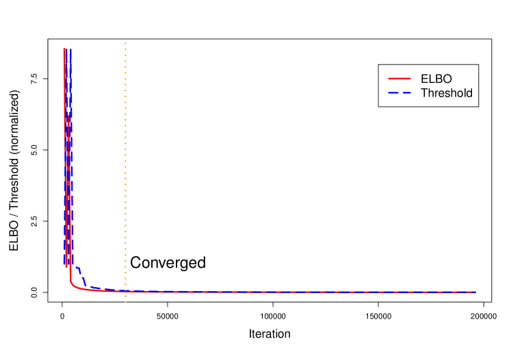
Figure 2: Runtime ELBO (solid) and threshold delta (dashed) for all iterations. ELBO and threshold have been normalized to the same scale. We can see there is a diminishing return after about 30,000 iterations (vertical dotted line). In this example the algorithm ran for over a day longer than it needed to (on a Dell XPS computer with 8-cpu Intel core i9 and 64GB RAM memory) in finding the best posterior estimate it could generate.

3.4 Maximum Likelihood Approach

We used the R package clustMD  ²³ to compare a maximum likelihood (MLE) clustering approach to Bayesian LCA. clustMD employs a mixture of Gaussian distributions to model the latent variable and an Expectation Maximisation (EM) algorithm to estimate the latent cluster means. It also employs Monte Carlo EM for categorical data. clustMD supports mixed data so is appropriate in our context. To use clustMD the data must be reordered to have continuous variables first, followed by ordinal variables and then nominal variables. For our data the computational runtime was about 50% of JAGS MCMC, approximately 62 hours.

4 Results

A Dell XPS laptop with an 8 cpu Intel core i9 processor and 64GB memory was used for this work. The baseline results using the Northeast region subset of Optum^TM obtained from JAGS were close to the Hubbard et al. results (Table  LABEL:table:comp). The differences in biomarker shift can be explained by the wider patient geographic catchment and differences in missing data for PEDSnet and Optum^TM. Following these results we are confident in the extensibility of the model to the same disease area with different EHR data. Unfortunately the computational performance is poor using JAGS. For example, a subset of $\sim$38,000 observations taking 16 hours to run.

We tested posterior diagnostics, goodness of fit diagnostics and the empirical performance of the LCA model. Stan has comprehensive posterior diagnostics available via the posterior  ³ and bayesplot  ⁷ R packages. The loo R package ²⁶ provides goodness of fit diagnostics based on Pareto Smoothed Importance Sampling (PSIS)  ²⁷, leave-one-out cross-validation and the Watanabe-Akaike/Widely Applicable information criterion (WAIC)  ²², ²⁶.

4.1 Posterior Diagnostics

The posterior diagnostics plots for the biomarkers in Figure 3 show that, for (a) MCMC, we see no evidence of collinearity and the posterior means appear close to those we obtained with JAGS (b). The mcmc pairs plot for VB appears reasonable for HbA1c but not for the Glucose biomarker rpg_b_int prior. There appears to be correlation between the glucose priors. Since there is a single chain for VB there is only the top triangular set, which represents 100% of the posterior samples. This type of plot does not communicate the relative variances of the posteriors.

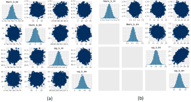
Figure 3: bayesplot pairs plots for (a) Stan HMC and (b) Stan VB for the two biomarkers. Each biomarker contains two model priors as defined in the model specification (Table  1). The b_int prior is the multivariate normal, $\beta^{Y}_{j}$ and the b_dm prior encodes known information on predictive accuracy containing values corresponding to a ROC AUC of 0.95. as described in Hubbard et al. Section 2.2 and 2.5 ¹⁵.

4.2 Goodness of fit

We used approximate leave-one-out cross-validation from the R loo package to evaluate the goodness of fit for the model. loo uses log-likelihood point estimates from the model to measure its predictive accuracy against training samples generated by Pareto Smoothed Importance Sampling (PSIS)  ²⁷. The PSIS shape parameter $k$ is used to assess the reliability of the estimate. If $k$ < 0.5 the variance of the importance ratios is finite and the central limit theorem holds. If $k$ is between 0.5 and 1 the variance of the importance ratios is infinite but the mean exists. If $k$ > 1 the variance and mean of the importance ratios do not exist. The results for the two biomarkers (Figure 4) show all of the n=38,000 observations are in a $k$ < 0.5 range. It appears VB performs approximately as well as MCMC in the context of the PSIS metric.

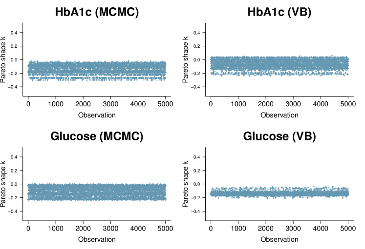
Figure 4: PSIS plots for the two biomarkers, HbA1c (top row) and Random Glucose (bottom row) under MCMC (left) and VB (right). Both biomarkers are well below $k$=0.5. The HbA1c biomarker is slightly worse for VB with a segment of observations above 0 but is well within good territory. The Random Glucose biomarker appears better in VB compared to MCMC but we know that the expected value obtained by VB for Glucose is not close to the true value obtained by MCMC.

4.3 Empirical Performance

The model mean estimates for biomarkers and the sensitivity analysis for the indicator variables show good agreement with JAGS apart from the Glucose variable under ADVI (Table  LABEL:table:allResults).

4.4 Maximum Likelihood Approach

For clustMD we take cluster 1 as the T2DM class as it is the minority cluster. The cluster means parallel coordinates plot in Figure 5 (a) indicates similar HbA1c (4.81) and Glucose (89.9) levels compared to the Bayesian model. Cluster 1 has a significantly larger variance (Figure 5) (b) possibly due to the high imbalance of T2DM in the data.

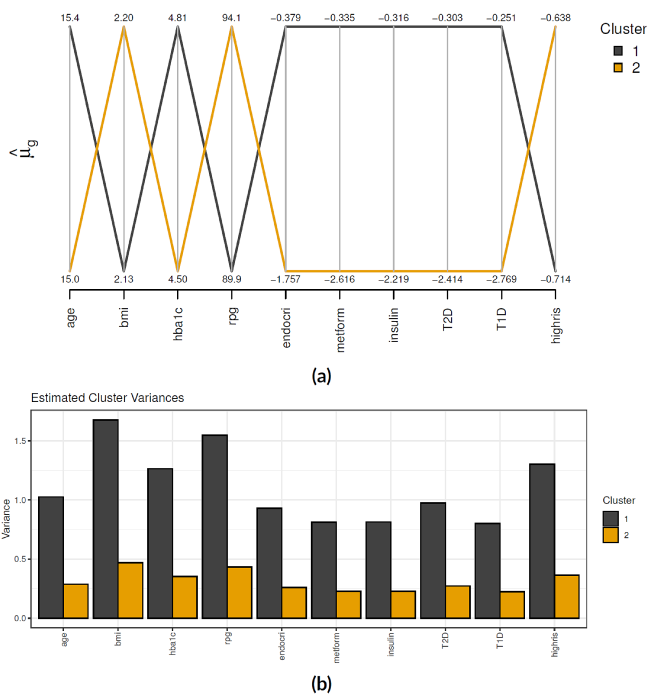
Figure 5: clustMD plots running 2 latent clusters. (a) shows a parallel coordinates plot for all variables, (b) shows the cluster variances for all variables.

5 Conclusions

We have demonstrated that this Hubbard et al. factorised form of the Bayes LCA model generalises to other EHR data. We believe this model form should also generalise to other disease areas. It can potentially become a uniquely useful tool for clinical decision support, especially for rare disease areas where gold-standard data is sparse. We have compared a number of alternative implementations of the model to identify if the intrinsic computation limitations from MCMC can be overcome in a real-world setting using VB. We have compared a range of methods for similar problems and set out practical guidance on implementing such models. We have investigated the challenges and suggest potential solutions for each of the alternative methods studied. For LCA, there are no closed-form implementations currently available so we need to use automatic "black box" approaches. We find automatic VB methods as implemented both for a baseline Pima Indian logistic model and in Stan VB are complex to configure and are very sensitive to model definition, algorithm hyperparameters and choice of gradient optimiser. The LCA model was significantly more challenging to implement but it was possible to achieve reasonable results. It might be possible to improve the Stan ADVI VB results after reparameterization of the model and use of Stan-specific helper functions so this is a potential next step. The baseline Pima Indian study showed that the conditionally conjugate mean-field closed-form approach to VB, even though it has many simplifying assumptions, performed best both computationally and in terms of posterior accuracy. We feel a redesign of the Bayes LCA EHR phenotyping model using an exponential family variational Bayes mixture model with Stochatic Variational Inference (SVI) could potentially address these issues. A closed-form approach also has the advantage that it can be published as an R/Python package, removing the need for clinical users to possess significant technical knowledge and perform time-consuming algorithm tuning needed for an automatic approach, or create complex LCA models in Stan.

6 Data Availability Statement

The EHR data used is proprietary to and licenced from Optum^TM. Our licence for use of these data lasted until September 2021. The model output data will be included with the R and Python scripts from our GitHub (https://github.com/buckleybrian/variationalBayesLCA). The Pima Indian data is publicly available from Kaggle at https://www.kaggle.com/datasets/uciml/pima-indians-diabetes-database.

References

- Alsowaida \BOthers. \APACyear2022 \APACinsertmetastaralsowaida2022vancomycin{APACrefauthors}Alsowaida, Y\BPBIS., Kubiak, D\BPBIW., Dionne, B., Kovacevic, M\BPBIP.\BCBL \BBA Pearson, J\BPBIC. \APACrefYearMonthDay2022. \BBOQ\APACrefatitleVancomycin Area under the Concentration-Time Curve Estimation Using Bayesian Modeling versus First-Order Pharmacokinetic Equations: A Quasi-Experimental Study Vancomycin area under the Concentration-time Curve Estimation using Bayesian modeling versus First-Order Pharmacokinetic Equations: A quasi-experimental study.\BBCQ \APACjournalVolNumPagesAntibiotics1191239. \PrintBackRefs\CurrentBib
- Boulanger \BBA Carlin \APACyear2021 \APACinsertmetastarboulanger703and{APACrefauthors}Boulanger, B.\BCBT \BBA Carlin, B\BPBIP. \APACrefYearMonthDay2021. \BBOQ\APACrefatitleHow and why Bayesian statistics are revolutionizing pharmaceutical decision making How and why Bayesian statistics are revolutionizing pharmaceutical decision making.\BBCQ \APACjournalVolNumPagesClinical Researcher70320. \PrintBackRefs\CurrentBib
- Bürkner \BOthers. \APACyear2023 \APACinsertmetastarrposterior2023{APACrefauthors}Bürkner, P\BHBIC., Gabry, J., Kay, M.\BCBL \BBA Vehtari, A. \APACrefYearMonthDay2023. \APACrefbtitleposterior: Tools for Working with Posterior Distributions. posterior: Tools for working with posterior distributions. {APACrefURL} https://mc-stan.org/posterior/ \APACrefnoteR package version 1.4.1 \PrintBackRefs\CurrentBib
- Carlin \BBA Nollevaux \APACyear2022 \APACinsertmetastarcarlin2022bayesian{APACrefauthors}Carlin, B\BPBIP.\BCBT \BBA Nollevaux, F. \APACrefYearMonthDay2022. \BBOQ\APACrefatitleBayesian complex innovative trial designs (CIDs) and their use in drug development for rare disease Bayesian complex innovative trial designs (CIDs) and their use in drug development for rare disease.\BBCQ \APACjournalVolNumPagesThe Journal of Clinical Pharmacology62S56–S71. \PrintBackRefs\CurrentBib
- Carpenter \BOthers. \APACyear2017 \APACinsertmetastarcarpenter2017stan{APACrefauthors}Carpenter, B., Gelman, A., Hoffman, M\BPBID., Lee, D., Goodrich, B., Betancourt, M.\BDBLRiddell, A. \APACrefYearMonthDay2017. \BBOQ\APACrefatitleStan: A probabilistic programming language Stan: A probabilistic programming language.\BBCQ \APACjournalVolNumPagesJournal of Statistical Software761. \PrintBackRefs\CurrentBib
- Dagenais \BOthers. \APACyear2022 \APACinsertmetastardagenais2022use{APACrefauthors}Dagenais, S., Russo, L., Madsen, A., Webster, J.\BCBL \BBA Becnel, L. \APACrefYearMonthDay2022. \BBOQ\APACrefatitleUse of real-world evidence to drive drug development strategy and inform clinical trial design Use of real-world evidence to drive drug development strategy and inform clinical trial design.\BBCQ \APACjournalVolNumPagesClinical Pharmacology & Therapeutics111177–89. \PrintBackRefs\CurrentBib
- Gabry \BBA Mahr \APACyear2017 \APACinsertmetastargabry2017bayesplot{APACrefauthors}Gabry, J.\BCBT \BBA Mahr, T. \APACrefYearMonthDay2017. \BBOQ\APACrefatitlebayesplot: Plotting for Bayesian models bayesplot: Plotting for bayesian models.\BBCQ \APACjournalVolNumPagesR package version10. \PrintBackRefs\CurrentBib
- Geman \BBA Geman \APACyear1984 \APACinsertmetastargeman1984stochastic{APACrefauthors}Geman, S.\BCBT \BBA Geman, D. \APACrefYearMonthDay1984. \BBOQ\APACrefatitleStochastic relaxation, Gibbs distributions, and the Bayesian restoration of images Stochastic relaxation, Gibbs distributions, and the Bayesian restoration of images.\BBCQ \APACjournalVolNumPagesIEEE Transactions on Pattern Analysis and Machine Intelligence6721–741. \PrintBackRefs\CurrentBib
- Geyer \APACyear1992 \APACinsertmetastargeyer1992practical{APACrefauthors}Geyer, C\BPBIJ. \APACrefYearMonthDay1992. \BBOQ\APACrefatitlePractical Markov Chain Monte Carlo Practical Markov Chain Monte Carlo.\BBCQ \APACjournalVolNumPagesStatistical science473–483. \PrintBackRefs\CurrentBib
- Hadjadj \BOthers. \APACyear2004 \APACinsertmetastarhadjadj2004prognostic{APACrefauthors}Hadjadj, S., Coisne, D., Mauco, G., Ragot, S., Duengler, F., Sosner, P.\BDBLMarechaud, R. \APACrefYearMonthDay2004. \BBOQ\APACrefatitlePrognostic value of admission plasma glucose and HbA1c in acute myocardial infarction Prognostic value of admission plasma glucose and HbA1c in acute myocardial infarction.\BBCQ \APACjournalVolNumPagesDiabetic Medicine214305–310. \PrintBackRefs\CurrentBib
- He \BOthers. \APACyear2023 \APACinsertmetastarhe2023trends{APACrefauthors}He, T., Belouali, A., Patricoski, J., Lehmann, H., Ball, R., Anagnostou, V.\BDBLBotsis, T. \APACrefYearMonthDay2023. \BBOQ\APACrefatitleTrends and Opportunities in Computable Clinical Phenotyping: A Scoping Review Trends and opportunities in computable clinical phenotyping: A scoping review.\BBCQ \APACjournalVolNumPagesJournal of Biomedical Informatics104335. \PrintBackRefs\CurrentBib
- Hoffman \BOthers. \APACyear2014 \APACinsertmetastarhoffman2014no{APACrefauthors}Hoffman, M\BPBID., Gelman, A.\BCBL \BOthersPeriod. \APACrefYearMonthDay2014. \BBOQ\APACrefatitleThe No-U-Turn sampler: adaptively setting path lengths in Hamiltonian Monte Carlo. The no-u-turn sampler: adaptively setting path lengths in hamiltonian monte carlo.\BBCQ \APACjournalVolNumPagesJ. Mach. Learn. Res.1511593–1623. \PrintBackRefs\CurrentBib
- Hornik \BOthers. \APACyear2003 \APACinsertmetastarplummer2003jags{APACrefauthors}Hornik, K., Leisch, F., Zeileis, A.\BCBL \BBA Plummer, M. \APACrefYearMonthDay2003. \BBOQ\APACrefatitleJAGS: A program for analysis of Bayesian graphical models using Gibbs sampling JAGS: A program for analysis of Bayesian graphical models using Gibbs sampling.\BBCQ \BIn \APACrefbtitleProceedings of the 3rd international workshop on distributed statistical computing Proceedings of the 3rd international workshop on distributed statistical computing (\BVOL 124, \BPGS 1–10). \PrintBackRefs\CurrentBib
- Hripcsak \BBA Albers \APACyear2013 \APACinsertmetastarhripcsak2013next{APACrefauthors}Hripcsak, G.\BCBT \BBA Albers, D\BPBIJ. \APACrefYearMonthDay2013. \BBOQ\APACrefatitleNext-generation phenotyping of Electronic Health Records Next-generation phenotyping of Electronic Health Records.\BBCQ \APACjournalVolNumPagesJournal of the American Medical Informatics Association201117–121. \PrintBackRefs\CurrentBib
- Hubbard \BOthers. \APACyear2019 \APACinsertmetastarhubbard2019bayesian{APACrefauthors}Hubbard, R\BPBIA., Huang, J., Harton, J., Oganisian, A., Choi, G., Utidjian, L.\BDBLChen, Y. \APACrefYearMonthDay2019. \BBOQ\APACrefatitleA Bayesian latent class approach for EHR-based phenotyping A Bayesian latent class approach for EHR-based phenotyping.\BBCQ \APACjournalVolNumPagesStatistics in Medicine38174–87. \PrintBackRefs\CurrentBib
- Hughes \BOthers. \APACyear2023 \APACinsertmetastarhughes2023fast{APACrefauthors}Hughes, D\BPBIM., García-Fiñana, M.\BCBL \BBA Wand, M\BPBIP. \APACrefYearMonthDay2023. \BBOQ\APACrefatitleFast approximate inference for multivariate longitudinal data Fast approximate inference for multivariate longitudinal data.\BBCQ \APACjournalVolNumPagesBiostatistics241177–192. \PrintBackRefs\CurrentBib
- Kucukelbir \BOthers. \APACyear2015 \APACinsertmetastarkucukelbir2015automatic{APACrefauthors}Kucukelbir, A., Ranganath, R., Gelman, A.\BCBL \BBA Blei, D. \APACrefYearMonthDay2015. \BBOQ\APACrefatitleAutomatic variational inference in Stan Automatic variational inference in Stan.\BBCQ \APACjournalVolNumPagesAdvances in Neural Information Processing Systems28. \PrintBackRefs\CurrentBib
- Kucukelbir \BOthers. \APACyear2017 \APACinsertmetastarkucukelbir2017automatic{APACrefauthors}Kucukelbir, A., Tran, D., Ranganath, R., Gelman, A.\BCBL \BBA Blei, D\BPBIM. \APACrefYearMonthDay2017. \BBOQ\APACrefatitleAutomatic differentiation variational inference Automatic differentiation variational inference.\BBCQ \APACjournalVolNumPagesJournal of Machine Learning Research. \PrintBackRefs\CurrentBib
- Kuczmarski \APACyear2002 \APACinsertmetastarkuczmarski20022000{APACrefauthors}Kuczmarski, R\BPBIJ. \APACrefYear2002. \APACrefbtitle2000 CDC Growth Charts for the United States: methods and development (No. 246) 2000 CDC Growth Charts for the United States: methods and development (no. 246) (\BNUM 246). \APACaddressPublisherDepartment of Health and Human Services, Centers for Disease Control and Prevention, National Center for Health Statistics. \PrintBackRefs\CurrentBib
- Lanza \BBA Rhoades \APACyear2013 \APACinsertmetastarlanza2013latent{APACrefauthors}Lanza, S\BPBIT.\BCBT \BBA Rhoades, B\BPBIL. \APACrefYearMonthDay2013. \BBOQ\APACrefatitleLatent class analysis: an alternative perspective on subgroup analysis in prevention and treatment Latent class analysis: an alternative perspective on subgroup analysis in prevention and treatment.\BBCQ \APACjournalVolNumPagesPrevention Science142157–168. \PrintBackRefs\CurrentBib
- Li \BOthers. \APACyear2020 \APACinsertmetastarli2020inferring{APACrefauthors}Li, Y., Nair, P., Lu, X\BPBIH., Wen, Z., Wang, Y., Dehaghi, A\BPBIA\BPBIK.\BDBLKellis, M. \APACrefYearMonthDay2020. \BBOQ\APACrefatitleInferring multimodal latent topics from electronic health records Inferring multimodal latent topics from electronic health records.\BBCQ \APACjournalVolNumPagesNature communications1112536. \PrintBackRefs\CurrentBib
- Magnusson \BOthers. \APACyear2020 \APACinsertmetastarmagnusson2020leave{APACrefauthors}Magnusson, M., Vehtari, A., Jonasson, J.\BCBL \BBA Andersen, M. \APACrefYearMonthDay2020. \BBOQ\APACrefatitleLeave-one-out cross-validation for Bayesian model comparison in large data Leave-one-out cross-validation for Bayesian model comparison in large data.\BBCQ \BIn \APACrefbtitleInternational Conference on Artificial Intelligence and Statistics International Conference on Artificial Intelligence and Statistics (\BPGS 341–351). \PrintBackRefs\CurrentBib
- McParland \BBA Gormley \APACyear2016 \APACinsertmetastarmcparland2016model{APACrefauthors}McParland, D.\BCBT \BBA Gormley, I\BPBIC. \APACrefYearMonthDay2016. \BBOQ\APACrefatitleModel based clustering for mixed data: clustMD Model based clustering for mixed data: clustMD.\BBCQ \APACjournalVolNumPagesAdvances in Data Analysis and Classification102155–169. \PrintBackRefs\CurrentBib
- Murphy \APACyear2012 \APACinsertmetastarmurphy2012machine{APACrefauthors}Murphy, K\BPBIP. \APACrefYear2012. \APACrefbtitleMachine learning: A Probabilistic Perspective Machine learning: A Probabilistic Perspective. \APACaddressPublisherMIT press. \PrintBackRefs\CurrentBib
- Song \BOthers. \APACyear2022 \APACinsertmetastarsong2022automatic{APACrefauthors}Song, Z., Hu, Y., Verma, A., Buckeridge, D\BPBIL.\BCBL \BBA Li, Y. \APACrefYearMonthDay2022. \BBOQ\APACrefatitleAutomatic phenotyping by a seed-guided topic model Automatic phenotyping by a seed-guided topic model.\BBCQ \BIn \APACrefbtitleProceedings of the 28th ACM SIGKDD Conference on Knowledge Discovery and Data Mining Proceedings of the 28th ACM SIGKDD Conference on Knowledge Discovery and Data Mining (\BPGS 4713–4723). \PrintBackRefs\CurrentBib
- Vehtari \BOthers. \APACyear2017 \APACinsertmetastarvehtari2017practical{APACrefauthors}Vehtari, A., Gelman, A.\BCBL \BBA Gabry, J. \APACrefYearMonthDay2017. \BBOQ\APACrefatitlePractical Bayesian model evaluation using leave-one-out cross-validation and WAIC Practical Bayesian model evaluation using leave-one-out cross-validation and WAIC.\BBCQ \APACjournalVolNumPagesStatistics and Computing2751413–1432. \PrintBackRefs\CurrentBib
- Vehtari \BOthers. \APACyear2015 \APACinsertmetastarvehtari2015pareto{APACrefauthors}Vehtari, A., Simpson, D., Gelman, A., Yao, Y.\BCBL \BBA Gabry, J. \APACrefYearMonthDay2015. \BBOQ\APACrefatitlePareto smoothed importance sampling Pareto smoothed importance sampling.\BBCQ \APACjournalVolNumPagesarXiv preprint arXiv:1507.02646. \PrintBackRefs\CurrentBib
- Wallace \BOthers. \APACyear2014 \APACinsertmetastarwallace2014optum{APACrefauthors}Wallace, P\BPBIJ., Shah, N\BPBID., Dennen, T., Bleicher, P\BPBIA.\BCBL \BBA Crown, W\BPBIH. \APACrefYearMonthDay2014. \BBOQ\APACrefatitleOptum Labs: Building a novel node in the learning health care system Optum Labs: Building a novel node in the learning health care system.\BBCQ \APACjournalVolNumPagesHealth Affairs3371187–1194. \PrintBackRefs\CurrentBib
- Xia \BBA Sheinson \APACyear2022 \APACinsertmetastarxia2022p30{APACrefauthors}Xia, Z.\BCBT \BBA Sheinson, D. \APACrefYearMonthDay2022. \BBOQ\APACrefatitleP30 Combining Real-World and Randomized Controlled Trial Survival Data Using Bayesian Methods P30 combining real-world and randomized controlled trial survival data using Bayesian methods.\BBCQ \APACjournalVolNumPagesValue in Health257S293. \PrintBackRefs\CurrentBib
- Yackulic \BOthers. \APACyear2020 \APACinsertmetastaryackulic2020need{APACrefauthors}Yackulic, C\BPBIB., Dodrill, M., Dzul, M., Sanderlin, J\BPBIS.\BCBL \BBA Reid, J\BPBIA. \APACrefYearMonthDay2020. \BBOQ\APACrefatitleA need for speed in Bayesian population models: a practical guide to marginalizing and recovering discrete latent states A need for speed in Bayesian population models: a practical guide to marginalizing and recovering discrete latent states.\BBCQ \APACjournalVolNumPagesEcological Applications305e02112. \PrintBackRefs\CurrentBib