Equilibrium Distributions for t-distributed Stochastic Neighbour Embedding

Abstract.

We study the empirical measure of the output of the t-distributed stochastic neighbour embedding algorithm when the initial data is given by $n$ independent, identically distributed inputs. We prove that under certain assumptions on the distribution of the inputs, this sequence of measures converges to an equilibrium distribution, which is described as a solution of a variational problem.

1. Introduction

First introduced in 2008 by van der Maaten and Hinton [14] as a variation over the earlier stochastic neighbour embedding (SNE) method[6], t-distributed stochastic neighbour embedding (t-SNE) is a dimension reduction technique that is particularly well-suited for visualization of high-dimensional datasets. This technique has seen a wide and phenomenal use of applications in a range of scientific disciplines, including biology [9, 8], engineering [5] and physics [15]. Despite the impressive empirical performance of t-SNE, and improvements in the implementation of the algorithm through various mechanisms [10, 7, 13] so far there has been relatively little progress in mathematics in trying to rigorously understand the theory behind t-SNE.

Questions such as “What happens when the initial dataset is pure noise?”, or “How strong should a signal be to visualize multiple clusters?” or “When does the method work (and why does it work so well)?” are surprisingly underdeveloped from a rigorous mathematical perspective. The goal of this paper is to address the first of these questions in the case where the number of data points diverges. Roughly speaking, in our main result, under some mild assumptions on the noise distribution, we prove the existence of an equilibrium measure (or a null-distribution) for t-SNE as the number of inputs goes to infinity.

Let $d,s\geq 2$ and $n\geq 1$. The goal of the t-SNE algorithm is to find a collection of vectors $Y_{1},\ldots,Y_{n}$ in $\mathbb{R}^{s}$ that is a low dimensional representation of input vectors $X_{1},\ldots,X_{n}\in\mathbb{R}^{d}$. This is done by constructing associated measures as follows. Given $X_{1},\ldots,X_{n}\in\mathbb{R}^{d}$, for $1\leq i,j\leq n$, we set

$$p_{j|i}=\frac{\exp(-\lVert X_{i}-X_{j}\rVert^{2}/2\sigma_{i}^{2})}{\sum_{k\neq i}\exp(-\lVert X_{i}-X_{k}\rVert^{2}/2\sigma_{i}^{2})},$$ (1.1)

where the sequence of numbers $\sigma_{i}$ satisfies for each $i=1,\ldots,n,$

$$-\sum_{j=1,j\neq i}^{n}p_{j|i}\log p_{j|i}=\log\text{Perp}.$$ (1.2)

The parameter $\text{Perp}=\text{Perp}(n)$ is called the perplexity of the model and we will assume that

$$\text{Perp}(n)=n\rho$$ (1.3)

for some $\rho\in(0,1)$. We then let for $1\leq i\neq j\leq n$,

$$p_{ij}=\frac{p_{i|j}+p_{j|i}}{2n}=\frac{1}{2n}\left(\frac{\exp(-\lVert X_{i}-X_{j}\rVert^{2}/2\sigma_{i}^{2})}{\sum_{k\neq i}\exp(-\lVert X_{i}-X_{k}\rVert^{2}/2\sigma_{i}^{2})}+\frac{\exp(-\lVert X_{i}-X_{j}\rVert^{2}/2\sigma_{j}^{2})}{\sum_{k\neq j}\exp(-\lVert X_{k}-X_{j}\rVert^{2}/2\sigma_{j}^{2})}\right),$$

and we set $p_{ii}=0$.

For a collection of vectors $Y_{1},\ldots,Y_{n}$ in $\mathbb{R}^{s}$ we define for $1\leq i\neq j\leq n,$

$$q_{ij}=\frac{(1+\lVert Y_{i}-Y_{j}\rVert^{2})^{-1}}{\sum_{k\neq\ell}(1+\lVert Y_{k}-Y_{\ell}\rVert^{2})^{-1}}.$$

and $q_{ii}=0$.

Last, we define for $X=(X_{1},\ldots,X_{n})\in(\mathbb{R}^{d})^{n}$ and $Y=(Y_{1},\ldots,Y_{n})\in\mathbb{(}\mathbb{R}^{s})^{n},$

$$L_{n,\rho}(X,Y)=\sum_{1\leq i\neq j\leq n}p_{ij}\log\left(\frac{p_{ij}}{q_{ij}}\right).$$ (1.4)

The function $L_{n,\rho}$ is the relative entropy between the probability distributions constructed from the collections $(p_{ij})_{1\leq i,j\leq n}$ and $(q_{ij})_{1\leq i,j\leq n}$. The output of t-SNE is the minimizer of 1.4:

$$Y^{*}=\operatorname*{arg\,min}_{Y\in(\mathbb{R}^{s})^{n}}L_{n,\rho}(X,Y).$$ (1.5)

Existence of solutions to the problems in 1.2 and 1.5 are discussed in Section 2.

We denote $\mathcal{M}(\mathbb{R}^{d})$ as the space of Borel probability measures on $\mathbb{R}^{d}$. Let $\mu_{X}\in\mathcal{M}(\mathbb{R}^{d})$ and $X_{1},\ldots,X_{n}$ be independent, identically distributed random variables with common probability measure $\mu_{X}$. Let $Y^{*}=(Y_{1},\dots,Y_{n})$ be the output given by t-SNE and define the empirical measure

$$\mu_{n}=\frac{1}{n}\sum_{i}\delta_{(X_{i},Y_{i})}\in\mathcal{M}(\mathbb{R}^{d}\times\mathbb{R}^{s}).$$ (1.6)

We now introduce the setup that describes the limit measures for the sequences $\mu_{n}$.

Let $\mu\in\mathcal{M}(\mathbb{R}^{d}\times\mathbb{R}^{s})$. For $\sigma\in\mathbb{R}$, $\rho\in(0,1)$ define $F_{\rho,\mu}:\mathbb{R}^{d}\times\mathbb{R}\to\mathbb{R}$ as

$$F_{\rho,\mu}(x,\sigma) =\int\frac{\exp(-\lVert x-x^{\prime}\rVert^{2}/2\sigma^{2})}{\int\exp(-\lVert x-x^{\prime}\rVert^{2}/2\sigma^{2})\,d\mu(x^{\prime})}\log\left(\frac{\exp(-\lVert x-x^{\prime}\rVert^{2}/2\sigma^{2})}{\int\exp(-\lVert x-x^{\prime}\rVert^{2}/2\sigma^{2})\,d\mu(x^{\prime})}\right)\,d\mu(x^{\prime})+\log\rho.$$

Note that the integrations above are on the space $\mathbb{R}^{d}\times\mathbb{R}^{s}$. The integrands are constant in the remaining last $s$ variables and the notation $d\mu(x^{\prime})$ is to highlight that we are integrating on the variable $x^{\prime}\in\mathbb{R}^{d}$.

Next, let $\sigma^{*}_{\rho,\mu}:\mathbb{R}^{d}\to\mathbb{R}$ be defined as the unique solution of the equation

$$F_{\rho,\mu}(x,\sigma^{*}_{\rho,\mu}(x))=0.$$ (1.7)

Existence, uniqueness and properties of $\sigma_{\rho,\mu}^{*}$ are established in Section 2.

Now, given a function $\psi:\mathbb{R}^{d}\to\mathbb{R}^{+}$, define the function $p_{\psi}:\mathbb{R}^{d}\times\mathbb{R}^{d}\to\mathbb{R}$ as

$$p_{\psi}(x,x^{\prime}) =\frac{1}{2}\left(\frac{\exp(-\lVert x-x^{\prime}\rVert^{2}/2\psi(x)^{2})}{\int\exp(-\lVert x-x^{\prime}\rVert^{2}/2\psi(x)^{2})\,d\mu(x^{\prime})}+\frac{\exp(-\lVert x-x^{\prime}\rVert^{2}/2\psi(x^{\prime})^{2})}{\int\exp(-\lVert x-x^{\prime}\rVert^{2}/2\psi(x^{\prime})^{2})\,d\mu(x)}\right)$$

and also let $q:\mathbb{R}^{s}\times\mathbb{R}^{s}\to\mathbb{R}$ be given by

$$q(y,y^{\prime})=\frac{(1+\lVert y-y^{\prime}\rVert^{2})^{-1}}{\iint(1+\lVert y-y^{\prime}\rVert^{2})^{-1}\,d\mu(y)d\mu(y^{\prime})}.$$ (1.8)

Lastly, define

$$I_{\rho}(\mu)=\iint p_{\sigma^{*}_{\rho,\mu}}(x,x^{\prime})\log\left(\frac{p_{\sigma^{*}_{\rho,\mu}}(x,x^{\prime})}{q(y,y^{\prime})}\right)\,d\mu(x,y)d\mu(x^{\prime},y^{\prime})$$ (1.9)

and for a given $\mu_{X}\in\mathcal{M}(\mathbb{R}^{d})$ write $\operatorname{\mathcal{P}}_{X}$ for the set of probability measures on $\mathbb{R}^{d}\times\mathbb{R}^{s}$ whose marginal coincides with $\mu_{X}$, that is,

$$\operatorname{\mathcal{P}}_{X}=\{\mu\in\mathcal{M}(\mathbb{R}^{d}\times\mathbb{R}^{s}):\text{the }\mathbb{R}^{d}\text{ marginal of }\mu\text{ is }\mu_{X}\}.$$

Moreover, define

$$\widetilde{\operatorname{\mathcal{P}}}_{X}=\left\{\mu\in\operatorname{\mathcal{P}}_{X}:\int(p(x,x^{\prime})-q(y,y^{\prime}))\frac{y-y^{\prime}}{1+\lVert y-y^{\prime}\rVert^{2}}\,d\mu(x^{\prime},y^{\prime})=0,\,\mu(x,y)\text{-a.e.}\right\}.$$

We can now state our main result.

Theorem 1.1.

Assume $\mu_{X}$ has a $C^{1}$ density $f(x)$ and compact support. Let $X_{i}\in\mathbb{R}^{d}$ be independent, identically distributed random variables with common distribution $\mu_{X}$. Then for any $\rho\in(0,1)$,

$$\lim_{n\to\infty}\inf_{Y}L_{n,\rho}(X,Y)=\inf_{\mu\in\widetilde{\operatorname{\mathcal{P}}}_{X}}I_{\rho}(\mu).$$

Moreover, there exist a measure $\mu^{*}$ and a sub-sequence $n_{k}$ such that $\mu_{n_{k}}$ converges weakly to $\mu^{*}$ and $I_{\rho}(\mu^{*})=\inf_{\mu\in\widetilde{\operatorname{\mathcal{P}}}_{X}}I_{\rho}(\mu)$.

We can also infer that the limiting measure has compact support.

Theorem 1.2.

Under the same assumptions of Theorem 1.1, $\mu^{*}$ has compact support.

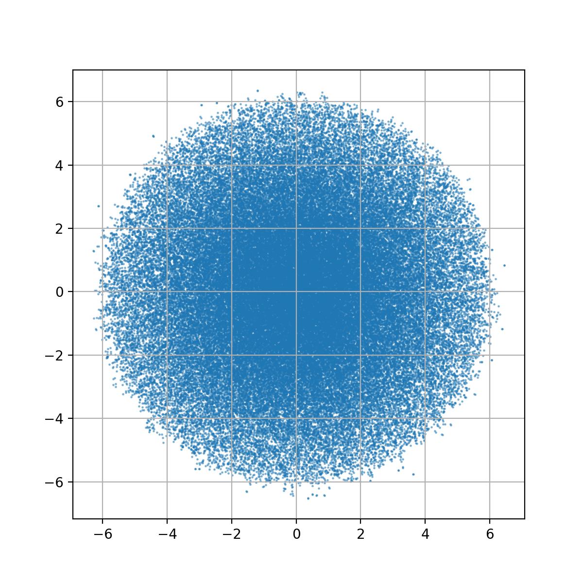
Figure 1. Simulation of a t-SNE output with $100,000$ independent input data distributed according to an uniform distribution on $[-1,1]^{d}$ in dimension $500$.

We conclude this section with some historical remarks and a brief description on the structure of the paper. As far as we know, Theorem 1.1 is the first result in the literature that characterizes the null distribution of t-SNE. Given the exceptional empirical performance of t-SNE, it is surprising to us that theoretical results are still scarce. Significant achievements were made by Linderman and Steinerberger [11] after earlier work by Shaham and Steinerberger [12], who gave conditions under which the algorithm successfully separates clusters (in a suitably formal sense). More exploration on this question was performed by Arora, Hu and Kothari [1] who studied performance of the gradient descent performed by t-SNE under certain deterministic conditions on the ground-truth clusters. More recently, Cai and Ma [3] formalized and made rigorous an observation first made by Linderman and Steinerberger [11]: a relationship to spectral clustering when t-SNE is ran in what is called the early exaggeration phase. For a comprehensive survey on other aspects of stochastic neighbor embeddings and their relationship to other dimension reduction techniques readers are invited to check Chapter 15 in [4] and the references therein.

The paper is organized as follows. In the next section, we show existence and uniqueness of the solution of 1.7. This section is where we use the assumptions of a $C^{1}$ density and compact support on $\mu_{X}$. In Section 3, we show uniform convergence of the sum 1.4 towards $F_{\rho,\mu}$ and in Section 4, we prove Theorem 1.1. Theorem 1.2 is proven in Section 5. The Appendix contains a separate analysis of the space $\widetilde{\operatorname{\mathcal{P}}}_{X}$ which may be of independent interest.

1.1. Acknowledgments

Antonio Auffinger’s research is partially supported by NSF Grant CAREER DMS-1653552, Simons Foundation/SFARI (597491-RWC), and NSF Grant 2154076. Daniel Fletcher’s research is partially supported by the Simons Foundation/SFARI (597491-RWC). Both authors would like to thank Eric Johnson, Madhav Mani, and William Kath for inspiring discussions on dimension reduction methods.

2. Existence and properties of $F_{\rho,\mu}$, $\sigma^{*}_{\rho,\mu}$

In this section, we establish existence and uniqueness of solutions of the problem 1.7.

Note that $F_{\rho,\mu}$ is $C^{\infty}$ and we can write

$$F_{\rho,\mu}(x,\sigma)= -\int\frac{\lVert x-x^{\prime}\rVert^{2}}{2\sigma^{2}}\frac{\exp(-\lVert x-x^{\prime}\rVert^{2}/2\sigma^{2})}{\int\exp(-\lVert x-x^{\prime}\rVert^{2}/2\sigma^{2})\,d\mu(x^{\prime})}\,d\mu(x^{\prime})$$

$$-\log\left(\int\exp(-\lVert x-x^{\prime}\rVert^{2}/2\sigma^{2})\,d\mu(x^{\prime})\right)+\log\rho.$$

2.1. Uniqueness and smoothness of $\sigma^{*}_{\rho,\mu}$

We start with the following Lemma that establishes lower bounds for $F_{\rho,\mu}$.

Lemma 1.

If $\mu$ has a $C^{1}$ density $f$ such that both $f$ and $\lVert\nabla f\rVert$ are bounded then there exists a constant $C>0$ so that

$$F_{\rho,\mu}(x,\sigma)\geq-C\log\sigma-\log f(x)+\log\rho.$$

In particular, $F_{\rho,\mu}(x,\sigma)\to\infty$ as $\sigma\to 0$.

Proof.

First note that

$$\int\exp(-\lVert x-x^{\prime}\rVert^{2}/2\sigma^{2})\,d\mu(x^{\prime}) =\left(2\pi\sigma^{2}\right)^{d/2}\int\frac{e^{-\lVert x-x^{\prime}\rVert^{2}/2\sigma^{2}}}{\left(2\pi\sigma^{2}\right)^{d/2}}f(x^{\prime})\,dx^{\prime}=\left(2\pi\sigma^{2}\right)^{d/2}\mathbb{E}_{x,\sigma}f(X^{\prime})$$

where the expectation is over a $N(x,\sigma I)$ random variable. As $\sigma\to 0$, these Gaussian measures converge weakly to $\delta_{x}$. Hence since $f$ is continuous and bounded $\mathbb{E}f(X^{\prime})\to f(x)$. In particular, for some $\varepsilon(\sigma)$ that tends to 0 as $\sigma\to 0$, we have

$$-\log\int\exp(\lVert x-x^{\prime}\rVert^{2}/2\sigma^{2})\,d\mu(x^{\prime}) =-\frac{d}{2}\log(2\pi\sigma^{2})-\log f(x)+\varepsilon(\sigma)$$

$$\geq-C\log\sigma-\log f(x).$$ (2.1)

Now using integration by parts, for all $x$ in the support of $\mu$ (so that $f(x)>0$), we have:

$$\quad\frac{\int\frac{\lVert x-x^{\prime}\rVert^{2}}{2\sigma^{2}}\exp(-\lVert x-x^{\prime}\rVert^{2}/2\sigma^{2})\,d\mu(x^{\prime})}{\int\exp(-\lVert x-x^{\prime}\rVert^{2}/2\sigma^{2})\,d\mu(x^{\prime})}$$

$$=-\frac{\frac{1}{4}\int\nabla\lVert x-x^{\prime}\rVert^{2}\cdot\nabla\exp(-\lVert x-x^{\prime}\rVert^{2}/2\sigma^{2})f(x^{\prime})\,dx^{\prime}}{\int\exp(-\lVert x-x^{\prime}\rVert^{2}/2\sigma^{2})f(x^{\prime})\,dx^{\prime}}$$

$$=\frac{1}{4}\frac{\int\exp(-\lVert x-x^{\prime}\rVert^{2}/2\sigma^{2})\left(\nabla f(x^{\prime})\cdot\nabla\lVert x-x^{\prime}\rVert^{2}+f(x^{\prime})\Delta\lVert x-x^{\prime}\rVert^{2}\right)\,dx^{\prime}}{\int\exp(-\lVert x-x^{\prime}\rVert^{2}/2\sigma^{2})f(x^{\prime})\,dx^{\prime}}$$

$$=\frac{1}{2}\frac{\int\exp(-\lVert x-x^{\prime}\rVert^{2}/2\sigma^{2})\nabla f(x^{\prime})\cdot(x-x^{\prime})\,dx^{\prime}}{\int\exp(-\lVert x-x^{\prime}\rVert^{2}/2\sigma^{2})f(x^{\prime})\,dx^{\prime}}+\frac{d}{2}$$

$$=\frac{1}{2}\frac{\mathbb{E}_{x,\sigma}\left[\nabla f(X^{\prime})\cdot(x-X^{\prime})\right]}{\mathbb{E}_{x,\sigma}f(X^{\prime})}+\frac{d}{2}$$

$$\to\frac{d}{2},$$

which combined with 2.1 ends the proof. ∎

For convenience, define

$$\widetilde{F}_{\rho,\mu}(x,\eta)=-\int\frac{\eta\lVert x-x^{\prime}\rVert^{2}\exp(-\eta\lVert x-x^{\prime}\rVert^{2})}{\int\exp(-\eta\lVert x-x^{\prime}\rVert^{2})\,d\mu(x^{\prime})}\,d\mu(x^{\prime})-\log\left(\int\exp(-\eta\lVert x-x^{\prime}\rVert^{2})\,d\mu(x^{\prime})\right)+\log\rho.$$

Then we have

$$F_{\rho,\mu}(x,\sigma)=\widetilde{F}_{\rho,\mu}(x,1/2\sigma^{2}).$$

Proposition 2.1.

Let $\mu\in\mathcal{M}(\mathbb{R}^{d})$ such that $\mu$ has a $C^{1}$ density $f$ such that both $f$ and $\lVert\nabla f\rVert$ are bounded. The equation $F_{\rho,\mu}(x,\sigma)=0$ has a unique solution $\sigma^{*}_{\rho,\mu}(x)$ for all $\rho\in(0,1)$ and $x\in\mathbb{R}^{d}$. Moreover, $x\mapsto\sigma^{*}_{\rho,\mu}(x)$ is smooth.

Proof.

Note that

$$\partial_{\eta}\widetilde{F}_{\rho,\mu}(x,\eta) =-\int\frac{\lVert x-x^{\prime}\rVert^{2}\exp(-\eta\lVert x-x^{\prime}\rVert^{2})}{\int\exp(-\eta\lVert x-x^{\prime}\rVert^{2})\,d\mu(x^{\prime})}\,d\mu(x^{\prime})+\int\frac{\eta\lVert x-x^{\prime}\rVert^{4}\exp(-\eta\lVert x-x^{\prime}\rVert^{2})}{\int\exp(-\eta\lVert x-x^{\prime}\rVert^{2})\,d\mu(x^{\prime})}\,d\mu(x^{\prime})$$

$$\quad-\eta\frac{\left(\int\lVert x-x^{\prime}\rVert^{2}\exp(-\eta\lVert x-x^{\prime}\rVert^{2})\,d\mu(x^{\prime})\right)^{2}}{\left(\int\exp(-\eta\lVert x-x^{\prime}\rVert^{2})\,d\mu(x^{\prime})\right)^{2}}+\frac{\int\lVert x-x^{\prime}\rVert^{2}\exp(-\eta\lVert x-x^{\prime}\rVert^{2})\,d\mu(x^{\prime})}{\int\exp(-\eta\lVert x-x^{\prime}\rVert^{2})\,d\mu(x^{\prime})}$$

$$=\eta\left(\int\frac{\lVert x-x^{\prime}\rVert^{4}\exp(-\eta\lVert x-x^{\prime}\rVert^{2})}{\int\exp(-\eta\lVert x-x^{\prime}\rVert^{2})\,d\mu(x^{\prime})}\,d\mu(x^{\prime})-\frac{\left(\int\lVert x-x^{\prime}\rVert^{2}\exp(-\eta\lVert x-x^{\prime}\rVert^{2})\,d\mu(x^{\prime})\right)^{2}}{\left(\int\exp(-\eta\lVert x-x^{\prime}\rVert^{2})\,d\mu(x^{\prime})\right)^{2}}\right).$$

Above, we can differentiate under the integral by Dominated Convergence Theorem.

Applying Cauchy-Schwarz with

$$f(x^{\prime})=\frac{\lVert x-x^{\prime}\rVert^{2}\exp(-\eta\lVert x-x^{\prime}\rVert^{2}/2)}{\left(\int\exp(-\eta\lVert x-x^{\prime}\rVert^{2})\,d\mu(x^{\prime})\right)^{1/2}},\quad g(x^{\prime})=\frac{\exp(-\eta\lVert x-x^{\prime}\rVert^{2}/2)}{\left(\int\exp(-\eta\lVert x-x^{\prime}\rVert^{2})\,d\mu(x^{\prime})\right)^{1/2}}$$

we see that $\partial_{\eta}\widetilde{F}_{\rho,\mu}\geq 0$ with equality if and only if $\eta=0$.

Now,

$$\partial_{\sigma}F_{\rho,\mu}(x,\sigma)=-\frac{1}{\sigma^{3}}\partial_{\eta}\widetilde{F}_{\rho,\mu}(x,1/2\sigma^{2}).$$

So we see that $\partial_{\sigma}F_{\rho,\mu}\leq 0$ for all $\sigma\neq 0$. Moreover, we have

$$\lim_{\sigma\to\infty}F_{\rho,\mu}(x,\sigma)=\log\rho<0.$$

By Lemma 1 above

$$\lim_{\sigma\to 0}F_{\rho,\mu}(x,\sigma)=\infty$$

so there exists unique $\sigma(x)=\sigma^{*}_{\rho,\mu}(x)$ such that $F_{\rho,\mu}(x,\sigma^{*}_{\rho,\mu}(x))=0$. Moreover, by the implicit function theorem, $\sigma^{*}_{\rho,\mu}:\mathbb{R}^{d}\to\mathbb{R}$ is smooth. ∎

3. Uniform convergence of $F_{\rho,\mu_{n}}(x,\sigma)$

Recall the empirical measures $\mu_{n}$ defined in 1.6. In this section, we establish uniform convergence of $F_{\rho,\mu_{n}}(x,\sigma)$. This result is useful in its own right and holds under the lighter assumption that $\mu$ has sub-Gaussian tails. To lighten the notation, we will remove the subscript $\rho$ from $F_{\rho,\mu_{n}}(x,\sigma)$. We start this section with some lemmas on measures with sub-Gaussian tails.

Recall that we say that a measure $\nu$ on $\mathbb{R}$ has sub-Gaussian tails if there is a positive constant $C$ such that $\nu((t,\infty))\leq 2\exp(-Ct^{2})$.

Lemma 2.

Let $\nu$ be sub-Gaussian with second moment equal to 1 and suppose $X\in\mathbb{R}^{d}$ has i.i.d. entries drawn from $\nu$. Then there exists $C,c_{1}$ such that

$$\mathbb{P}\left(\lVert X\rVert\geq\sqrt{d}+t\right)\leq Ce^{-c_{1}t^{2}}.$$

Proof.

Since $X_{1},\dots,X_{d}$ are sub-Gaussian, $X_{i}^{2}-1$ is sub-exponential for each $1\leq i\leq d$. It follows from Bernstein’s inequality [2, Corollary 2.11] that we have

$$\mathbb{P}\left(\left|\frac{1}{d}\lVert X\rVert^{2}-1\right|\geq u\right)\leq C\exp\left(-c_{1}d\min(u,u^{2})\right).$$

Now, note that for all $z\geq 0$, $\lvert z-1\rvert\geq a$ implies that $\lvert z^{2}-1\rvert\geq\max(a,a^{2})$ (separate into cases $a\leq 1,a\geq 1$). In particular, by the above tail inequality with $u=\max(a,a^{2})$, we have

$$\mathbb{P}\left(\left|\frac{1}{\sqrt{d}}\lVert X\rVert-1\right|\geq a\right)\leq C\exp\left(-c_{1}da^{2}\right).$$

Setting $t=a\sqrt{d}$ we see that

$$\mathbb{P}\left(\lVert X\rVert\geq\sqrt{d}+t\right)\leq Ce^{-c_{1}t^{2}}.$$

∎

Lemma 3.

Let $\nu$ be sub-Gaussian and $c_{1}$ be the constant from Lemma 2. Let $X_{1},\dots,X_{n}\in\mathbb{R}^{d}$ have i.i.d. entries drawn from $\nu$. Then there exists a constant $C$ such that

$$\mathbb{P}\left(\max_{i=1,\dots,n}\lVert X_{i}\rVert\geq\sqrt{\frac{\log n}{c_{1}}}+\sqrt{d}+t\right)\leq Ce^{-c_{1}t^{2}}.$$

Proof.

By Lemma 2, we have

$$\mathbb{P}\left(\max_{i=1,\dots,n}\lVert X_{i}\rVert\geq\sqrt{d}+u\right) \leq\sum_{i}\mathbb{P}\left(\lVert X_{i}\rVert\geq\sqrt{d}+u\right)$$

$$=n\mathbb{P}\left(\lVert X_{1}\rVert\geq\sqrt{d}+u\right)$$

$$\leq Cne^{-c_{1}u^{2}}.$$

Now, setting $u=\sqrt{\frac{\log n}{c_{1}}}+t$,

$$e^{-c_{1}u^{2}}\leq\frac{1}{n}e^{-c_{1}t^{2}}.$$

Hence

$$\mathbb{P}\left(\max_{i=1,\dots,n}\lVert X_{i}\rVert\geq\sqrt{\frac{\log n}{c_{1}}}+\sqrt{d}+t\right)\leq Ce^{-c_{1}t^{2}}.$$

∎

We will now state the main result of this section. For its proof we still need a few more Lemmas.

Proposition 3.1.

Let $\nu$ be sub-Gaussian and $c_{1}$ be a constant from Lemma 2. Let $X_{1},\dots,X_{n}\in\mathbb{R}^{d}$ have i.i.d. entries drawn from $\nu$ and let $\mu_{n}=\frac{1}{n}\sum\delta_{X_{i}}$. Let $\delta>0$ be a constant such that $c_{1}\delta^{2}>16$. Then, there exists $\epsilon>0$ such that almost surely in $X_{1},\dots,X_{n}$:

$$\sup_{\begin{subarray}{c}\sigma\in[\delta,\sqrt{n}]\\ i=1,\dots,n\end{subarray}}\left|F_{\mu_{n}}(X_{i},\sigma)-F_{\mu}(X_{i},\sigma)\right|=O(n^{-\epsilon}).$$

Lemma 4.

Suppose that $\varepsilon_{1},\dots,\varepsilon_{n}$ are i.i.d. Rademacher and let $B\subseteq\mathbb{R}^{n}$ be a finite set. Then

$$\mathbb{E}\sup_{b\in B}\sum_{i=1}^{n}\varepsilon_{i}b_{i}\leq\max_{b\in B}\lVert b\rVert_{2}\sqrt{2\log\lvert B\rvert}.$$

Proof of Lemma 4.

Let $\lambda\in\mathbb{R}$. Then

$$\exp\left(\lambda\mathbb{E}\sup_{b}\sum_{i=1}^{n}\varepsilon_{i}b_{i}\right)\leq\mathbb{E}\exp\left(\lambda\sup_{b}\sum_{i=1}^{n}\varepsilon_{i}b_{i}\right)=\mathbb{E}\sup_{b}\exp\left(\lambda\sum_{i=1}^{n}\varepsilon_{i}b_{i}\right)\leq\sum_{b}\mathbb{E}\exp\left(\lambda\sum_{i=1}^{n}\varepsilon_{i}b_{i}\right).$$

Now note that

$$\mathbb{E}\exp\left(\lambda\sum_{i=1}^{n}\varepsilon_{i}b_{i}\right)=\prod_{i}\mathbb{E}\exp\left(\lambda\varepsilon_{i}b_{i}\right)=\prod_{i}\cosh(\lambda b_{i})\leq\prod_{i}\exp\left(\frac{\lambda^{2}b_{i}^{2}}{2}\right)=\exp\left(\frac{\lambda^{2}\lVert b\rVert^{2}}{2}\right).$$

In particular, we see that

$$\exp\left(\lambda\mathbb{E}\sup_{b}\sum_{i=1}^{n}\varepsilon_{i}b_{i}\right)\leq\lvert B\rvert\exp\left(\frac{\lambda^{2}\max_{b}\lVert b\rVert^{2}}{2}\right)$$

and therefore

$$\mathbb{E}\sup_{b}\sum_{i=1}^{n}\varepsilon_{i}b_{i}\leq\frac{\log\lvert B\rvert}{\lambda}+\frac{\lambda\max_{b}\lVert b\rVert^{2}}{2}.$$

This upper bound is minimized at

$$\lambda=\frac{\sqrt{2\log\lvert B\rvert}}{\max_{b}\lVert b\rVert_{2}}$$

which gives

$$\mathbb{E}\sup_{b}\sum_{i=1}^{n}\varepsilon_{i}b_{i}\leq\max_{b\in B}\lVert b\rVert_{2}\sqrt{2\log\lvert B\rvert}.$$

∎

Lemma 5.

Let $\delta>0$ be constant, $K_{n}=[\delta,\sqrt{n}]$ and $h:\mathbb{R}^{d}\times\mathbb{R}^{d}\times\mathbb{R}\to\mathbb{R}$. Suppose the following hold:

• $\mu$ is sub-Gaussian,

• $h(x,x^{\prime},\sigma)$ is $C^{1}$ for all $x,x^{\prime}$ and all $\sigma\in K_{n}$,

• $h(x,x^{\prime},\sigma)$ and $\nabla_{x}h(x,x^{\prime},\sigma)$ are bounded for all $x,x^{\prime}$ and all $\sigma\in K_{n}$,

• $h(x,x^{\prime},\sigma)\to 0$ as $\lVert x-x^{\prime}\rVert/\sigma\to\infty$.

Let $X_{1},\dots,X_{n}$ be i.i.d. random variables drawn from $\mu$. Let $\mu_{n}=\frac{1}{n}\sum_{i}\delta_{X_{i}}$. Then for any $\varepsilon>0$ with probability at least $1-e^{-c\varepsilon^{2}n}$ we have

$$\sup_{\sigma\in K_{n},x}\left|\int h(x,x^{\prime},\sigma)\,d\mu_{n}(x^{\prime})-\int h(x,x^{\prime},\sigma)\,d\mu(x^{\prime})\right|\leq\varepsilon+O\left(\sqrt{\frac{\log n}{n}}\right).$$

Proof.

Let $\mathbb{E}$ be the expectation taken over the randomness in $X_{1},\dots,X_{n}$. We can write

$$\left|\int h(x,x^{\prime},\sigma)\,d\mu_{n}(x^{\prime})-\int h(x,x^{\prime},\sigma)\,d\mu(x^{\prime})\right| =\left|\frac{1}{n}\sum_{i}h(x,X_{i},\sigma)-\int h(x,x^{\prime},\sigma)\,d\mu(x^{\prime})\right|$$

$$=\left|\frac{1}{n}\sum_{i}h(x,X_{i},\sigma)-\mathbb{E}h(x,X_{i},\sigma)\right|.$$

Now, since $h$ is bounded, $\frac{1}{n}\sum_{i}h(x,X_{i},\sigma)-\mathbb{E}h(x,X_{i},\sigma)$ has bounded differences (as a function of $X_{1},\dots,X_{n}$) with $c_{i}=C/n$. Hence, by McDiarmid’s inequality [2, Theorem 6.2], with probability at least $1-e^{-c\varepsilon^{2}n}$, we have

$$\left|\frac{1}{n}\sum_{i}h(x,X_{i},\sigma)-\mathbb{E}h(x,X_{i},\sigma)\right| \leq\mathbb{E}\left|\frac{1}{n}\sum_{i}h(x,X_{i},\sigma)-\mathbb{E}h(x,X_{i},\sigma)\right|+\varepsilon$$

$$\leq\mathbb{E}\sup_{\sigma\in K_{n},x}\left|\frac{1}{n}\sum_{i}h(x,X_{i},\sigma)-\mathbb{E}h(x,X_{i},\sigma)\right|+\varepsilon.$$ (3.1)

Now, let $X^{\prime}_{i}$ be i.i.d. drawn from $\mu$ and independent from $X_{i}$ and let $\mathbb{E}^{\prime}$ be expectation over all of $X_{i}^{\prime}$. Then

$$\mathbb{E}\sup_{\sigma\in K_{n},x}\left|\frac{1}{n}\sum_{i}h(x,X_{i},\sigma)-\mathbb{E}h(x,X_{i},\sigma)\right| =\mathbb{E}\sup_{\sigma\in K_{n},x}\left|\frac{1}{n}\sum_{i}h(x,X_{i},\sigma)-\mathbb{E}^{\prime}h(x,X^{\prime}_{i},\sigma)\right|$$

$$=\mathbb{E}\sup_{\sigma\in K_{n},x}\left|\mathbb{E}^{\prime}\frac{1}{n}\sum_{i}h(x,X_{i},\sigma)-h(x,X^{\prime}_{i},\sigma)\right|$$

$$\leq\mathbb{E}\mathbb{E}^{\prime}\sup_{\sigma\in K_{n},x}\left|\frac{1}{n}\sum_{i}h(x,X_{i},\sigma)-h(x,X^{\prime}_{i},\sigma)\right|.$$

Let $\varepsilon_{i}$ be i.i.d. Rademacher distributed random variables. Then since $X_{i},X_{i}^{\prime}$ are i.i.d., $h(x,X_{i},\sigma)-h(x,X^{\prime}_{i},\sigma)$ and $\varepsilon_{i}(h(x,X_{i},\sigma)-h(x,X^{\prime}_{i},\sigma))$ have the same distribution. In particular, by the previous inequality:

$$\mathbb{E}\sup_{\sigma\in K_{n},x}\left|\frac{1}{n}\sum_{i}h(x,X_{i},\sigma)-\mathbb{E}h(x,X_{i},\sigma)\right| \leq\mathbb{E}\mathbb{E}^{\prime}\sup_{\sigma\in K_{n},x}\left|\frac{1}{n}\sum_{i}\varepsilon_{i}(h(x,X_{i},\sigma)-h(x,X^{\prime}_{i},\sigma))\right|$$

$$\leq 2\mathbb{E}\sup_{\sigma\in K_{n},x}\left|\frac{1}{n}\sum_{i}\varepsilon_{i}h(x,X_{i},\sigma)\right|$$

$$=2\mathbb{E}\mathbb{E}\left[\sup_{\sigma\in K_{n},x}\left|\frac{1}{n}\sum_{i}\varepsilon_{i}h(x,X_{i},\sigma)\right|\big{|}X_{1},\dots,X_{n}\right].$$

Let

$$H(x,\sigma)=\left|\frac{1}{n}\sum_{i}\varepsilon_{i}h(x,X_{i},\sigma).\right|$$

and $E=\left\{\max_{i=1,\dots,n}\lVert X_{i}\rVert\geq 2\sqrt{n}+\sqrt{\frac{\log n}{c_{1}}}\right\}$. Since $\mu$ is sub-Gaussian, by Lemma 3 with $t=\sqrt{n}$, there exists $C$ such that $\mathbb{P}(E)\leq Ce^{-c_{1}n}$.

Let $A^{(n)}=[-n,n]^{d}$. Then on $E^{c}$, for $x\notin A^{(n)}$ and $\sigma\in K_{n}$, we have $\frac{\lVert x-X_{i}\rVert}{\sigma}\geq\sqrt{n}/2$ and hence, by the decay condition on $h$, for sufficiently large $n$ we have

$$\sup_{x\in\mathbb{R}^{d},\sigma\in K_{n}}H(x,\sigma)=\sup_{x\in A^{(n)},\sigma\in K_{n}}H(x,\sigma).$$

Since $A^{(n)}\times K_{n}$ is compact and $H(x,\sigma)$ is continuous, $\sup_{x\in A^{(n)},\sigma\in K_{n}}H(x,\sigma)$ is achieved at some $(x^{*},\sigma^{*})$. Let $A^{(n)}_{k}=A^{(n)}\cap\frac{1}{k}\mathbb{Z}^{d}$ and let $x_{k}\in A^{(n)}_{k}$ be the closest point in $A^{(n)}_{k}$ to $x^{*}$. Then, using the fact that $\nabla_{x}h(x,x^{\prime},\sigma)$ is bounded:

$$\left|\sup_{\sigma\in K_{n},x\in A^{(n)}}H(x,\sigma)-\sup_{x\in A_{k}^{(n)}}H(x,\sigma^{*})\right| =H(x^{*},\sigma^{*})-\sup_{x\in A_{k}^{(n)}}H(x,\sigma^{*})$$

$$\leq H(x^{*},\sigma^{*})-H(x_{k},\sigma^{*})$$

$$\leq\sup_{x\in A^{(n)}}\lVert\nabla_{x}H(x,\sigma^{*})\rVert\,\lVert x^{*}-x_{k}\rVert$$

$$=O\left(\frac{1}{\sqrt{k}}\right).$$

Hence combining the above inequalities, and using the fact that $h$ is bounded, we have

$$\mathbb{E}\left[\sup_{x\in\mathbb{R}^{d},\sigma\in K_{n}}\left|\frac{1}{n}\sum_{i}h(x,X_{i},\sigma)-\mathbb{E}h(x,X_{i},\sigma)\right|\right]$$

$$\leq\, 2\mathbb{E}\mathbb{E}\left[\textbf{\rm{1}}_{E^{c}}\sup_{x\in A^{(n)}_{k}}\left|\frac{1}{n}\sum_{i}\varepsilon_{i}h(x,X_{i},\sigma^{*})\right|\big{|}X_{1},\dots,X_{n}\right]+O\left(\frac{1}{\sqrt{k}}\right)+C\mathbb{P}(E).$$

Now apply Lemma 4 with

$$B=\left\{\left(\frac{1}{n}h(a,X_{i},\sigma^{*})\right)_{i=1,\dots,n}:a\in A^{(n)}_{k}\right\}.$$

Then $\lvert B\rvert\leq\lvert A^{(n)}_{k}\rvert=(2nk)^{d}$ and since $h$ is bounded, $\max_{b\in B}\lVert b\rVert_{2}=O\left(\frac{1}{\sqrt{n}}\right)$. It follows that

$$\mathbb{E}\left[\textbf{\rm{1}}_{E^{c}}\sup_{x\in A^{(n)}_{k}}\left|\frac{1}{n}\sum_{i}\varepsilon_{i}h(x,X_{i},\sigma^{*})\right|\big{|}X_{1},\dots,X_{n}\right]\leq C\sqrt{\frac{d\log(nk)}{n}}.$$

Taking $k=n$ we have

$$\mathbb{E}\left[\sup_{x\in\mathbb{R}^{d},\sigma\in K_{n}}\left|\frac{1}{n}\sum_{i}h(x,X_{i},\sigma)-\mathbb{E}h(x,X_{i},\sigma)\right|\right]=O\left(\sqrt{\frac{d\log n}{n}}\right)+O\left(\frac{1}{\sqrt{n}}\right)+Ce^{-cn}=O\left(\sqrt{\frac{\log n}{n}}\right).$$

In particular, combining this bound with 3, with probability at least $1-e^{-c\varepsilon^{2}n}$,

$$\sup_{x\in\mathbb{R}^{d},\sigma\in K_{n}}\left|\frac{1}{n}\sum_{i}h(x,X_{i},\sigma)-\mathbb{E}h(x,X_{i},\sigma)\right|\leq\varepsilon+O\left(\sqrt{\frac{\log n}{n}}\right).$$

∎

Define

$$f_{\sigma}(x,x^{\prime})=\exp\left(-\lVert x-x^{\prime}\rVert^{2}/2\sigma^{2}\right),\quad g_{\sigma}(x,x^{\prime})=\frac{\lVert x-x^{\prime}\rVert^{2}}{2\sigma^{2}}\exp\left(-\lVert x-x^{\prime}\rVert^{2}/2\sigma^{2}\right).$$ (3.2)

Lemma 6.

Let $c_{1}$ be the decay constant from Lemma 2 and let $\delta>0$. Then, almost surely in $X_{1},\dots,X_{n}$,

$$\sup_{\begin{subarray}{c}\sigma\in[\delta,\sqrt{n}]\\ i=1,\dots,n\end{subarray}}\left|\frac{\int g_{\sigma}(X_{i},x^{\prime})\,d\mu_{n}(x^{\prime})}{\int f_{\sigma}(X_{i},x^{\prime})\,d\mu_{n}(x^{\prime})}-\frac{\int g_{\sigma}(X_{i},x^{\prime})\,d\mu(x^{\prime})}{\int f_{\sigma}(X_{i},x^{\prime})\,d\mu(x^{\prime})}\right|=O(n^{8/c_{1}\delta^{2}-1/2}\sqrt{\log n}).$$

Proof.

First note that

$$\left|\frac{\int g_{\sigma}(x,x^{\prime})\,d\mu_{n}(x^{\prime})}{\int f_{\sigma}(x,x^{\prime})\,d\mu_{n}(x^{\prime})}\right. \left.-\frac{\int g_{\sigma}(x,x^{\prime})\,d\mu(x^{\prime})}{\int f_{\sigma}(x,x^{\prime})\,d\mu(x^{\prime})}\right|\leq\left|\frac{\int g_{\sigma}(x,x^{\prime})\,d\mu_{n}(x^{\prime})-\int g_{\sigma}(x,x^{\prime})\,d\mu(x^{\prime})}{\int f_{\sigma}(x,x^{\prime})\,d\mu_{n}(x^{\prime})}\right|$$

$$+\left|\frac{\int g_{\sigma}(x,x^{\prime})\,d\mu(x^{\prime})\left(\int f_{\sigma}(x,x^{\prime})\,d\mu_{n}(x^{\prime})-\int f_{\sigma}(x,x^{\prime})\,d\mu(x^{\prime})\right)}{\int f_{\sigma}(x,x^{\prime})\,d\mu(x^{\prime})\int f_{\sigma}(x,x^{\prime})\,d\mu_{n}(x^{\prime})}\right|.$$

First we want to bound the terms in the denominators. The terms in the numerators are dealt with using Lemma 5. Let $\alpha>0$. Define

$$E_{1}^{\prime}=\left\{\max_{i=1,\dots,n}\lVert X_{i}\rVert\geq\sqrt{\left(\alpha+\frac{1}{c_{1}}\right)}\sqrt{\log n}+\sqrt{d}\right\}.$$

Setting $t=\sqrt{\alpha\log n}$ in Lemma 3, we have $\mathbb{P}(E_{1}^{\prime})\leq Cn^{-c_{1}\alpha}$. To absorb the $\sqrt{d}$ term in $E_{1}^{\prime}$, we can find $\epsilon_{n}\to 0$ such that

$$E_{1}:=\left\{\max_{i=1,\dots,n}\lVert X_{i}\rVert\geq\sqrt{\alpha+\frac{1}{c_{1}}+\epsilon_{n}}\sqrt{\log n}\right\}$$

has $\mathbb{P}(E_{1})\leq Cn^{-c_{1}\alpha}$.

On $E_{1}^{c}$ for all $i,j$, we have

$$\lVert X_{i}-X_{j}\rVert^{2}\leq 4\left(\alpha+\frac{1}{c_{1}}+\epsilon_{n}\right)\log n=:4\gamma\log n.$$

Then, for $\sigma\in[\delta,\sqrt{n}]$, on $E_{1}^{c}$ for all $i$ we have

$$\int f_{\sigma}(X_{i},x^{\prime})\,d\mu_{n}(x^{\prime})=\int\exp\left(-\lVert X_{i}-x^{\prime}\rVert^{2}/2\sigma^{2}\right)\,d\mu_{n}(x^{\prime})\geq\exp\left(-\frac{2\gamma\log n}{\delta^{2}}\right)=n^{-2\gamma/\delta^{2}}.$$

Similarly, applying Lemma 2 with $t=\sqrt{\alpha\log n}$, for all $i$ we have that

$$\int f_{\sigma}(X_{i},x^{\prime})\,d\mu(x^{\prime}) \geq\left(1-Cn^{-c_{1}\alpha}\right)\exp\left(-\frac{2\gamma\log n}{\delta^{2}}\right)\geq\frac{1}{2}\exp\left(-\frac{2\gamma\log n}{\delta^{2}}\right)=\frac{1}{2}n^{-2\gamma/\delta^{2}}.$$

From Lemma 5 applied to $h=f_{\sigma}$ and $h=g_{\sigma}$, we can find $E_{2}$ with $\mathbb{P}(E_{2})\leq 2e^{-c\varepsilon^{2}n}$, such that, on $E_{2}^{c}$,

$$\sup_{\begin{subarray}{c}\sigma\in[\delta,\sqrt{n}]\\ i=1,\dots,n\end{subarray}}\left|\int f_{\sigma}(X_{i},x^{\prime})\,d\mu_{n}(x^{\prime})-\int f_{\sigma}(X_{i},x^{\prime})\,d\mu(x^{\prime})\right|$$

$$\quad+\sup_{\begin{subarray}{c}\sigma\in[\delta,\sqrt{n}]\\ i=1,\dots,n\end{subarray}}\left|\int g_{\sigma}(X_{i},x^{\prime})\,d\mu_{n}(x^{\prime})-\int g_{\sigma}(X_{i},x^{\prime})\,d\mu(x^{\prime})\right|\leq\,\varepsilon+O\left(\frac{\sqrt{\log n}}{\sqrt{n}}\right).$$

Hence, on $E_{1}^{c}\cap E_{2}^{c}$, combining the inequalities above,

$$\sup_{\begin{subarray}{c}\sigma\in[\delta,\sqrt{n}]\\ i=1,\dots,n\end{subarray}}\left|\frac{\int g_{\sigma}(X_{i},x^{\prime})\,d\mu_{n}(x^{\prime})}{\int f_{\sigma}(X_{i},x^{\prime})\,d\mu_{n}(x^{\prime})}-\frac{\int g_{\sigma}(X_{i},x^{\prime})\,d\mu(x^{\prime})}{\int f_{\sigma}(X_{i},x^{\prime})\,d\mu(x^{\prime})}\right|\leq C\varepsilon n^{4\gamma/\delta^{2}}+O\left(\frac{\sqrt{\log n}}{n^{1/2-4\gamma/\delta^{2}}}\right).$$

Now, in order for the RHS to converge to zero, we need

$$\varepsilon n^{4\gamma/\delta^{2}}\to 0,\quad 1/2-4\gamma/\delta^{2}>0.$$

Moreover, we have $\mathbb{P}(E_{1}\cup E_{2})\leq Cn^{-c_{1}\alpha}+2e^{-c\varepsilon^{2}n}$. Set $\varepsilon=n^{-\eta}$ for some $\eta>0$. In order to apply Borel–Cantelli to get almost sure convergence, we want

$$c_{1}\alpha>1,\quad 1-2\eta>0.$$

Hence we need to satisfy the following collection of inequalities:

$$\frac{4\gamma}{\delta^{2}}-\eta<0,\quad\frac{4\gamma}{\delta^{2}}-1/2<0,\quad c_{1}\alpha>1,\quad 1-2\eta >0.$$

Note that the last inequality gives $\eta<1/2$ and hence the first inequality implies the second. Now, recalling the definition of $\gamma$, the above is equivalent to

$$4\left(\alpha+\frac{1}{c_{1}}+\epsilon_{n}\right)<\eta\delta^{2},\quad c_{1}\alpha>1,\quad 0<\eta<1/2,$$

where we are free to choose $\alpha,\eta$, but $c_{1}$ and $\delta$ are fixed.

Let $\epsilon>0$ (which may change from line to line below) and set

$$\alpha=\frac{1}{c_{1}}+\epsilon,\quad\eta=\frac{1}{2}-\epsilon$$

Then all we require is that $\frac{8}{c_{1}\delta^{2}}+\epsilon<\frac{1}{2}-\epsilon.$ Equivalently,

$$\frac{8}{c_{1}\delta^{2}}-\frac{1}{2}<0.$$

When this condition is satisfied, we have:

$$\sup_{\begin{subarray}{c}\sigma\in[\delta,\sqrt{n}]\\ i=1,\dots,n\end{subarray}}\left|\frac{\int g_{\sigma}(X_{i},x^{\prime})\,d\mu_{n}(x^{\prime})}{\int f_{\sigma}(X_{i},x^{\prime})\,d\mu_{n}(x^{\prime})}-\frac{\int g_{\sigma}(X_{i},x^{\prime})\,d\mu(x^{\prime})}{\int f_{\sigma}(X_{i},x^{\prime})\,d\mu(x^{\prime})}\right|=O\left(n^{8/c_{1}\delta^{2}-1/2}\sqrt{\log n}\right).$$

∎

Lemma 7.

Let $c_{1}$ be the decay constant from Lemma 2 and let $\delta>0$ be such that $c_{1}\delta^{2}>8$. Then almost surely in $X_{1},\dots,X_{n}$,

$$\sup_{\begin{subarray}{c}\sigma\in[\delta,\sqrt{n}]\\ i=1,\dots,n\end{subarray}}\left|\log\left(\int f_{\sigma}(X_{i},x^{\prime})\,d\mu_{n}(x^{\prime})\right)-\log\left(\int f_{\sigma}(X_{i},x^{\prime})\,d\mu(x^{\prime})\right)\right|=O(n^{4/c_{1}\delta^{2}-1/2}\sqrt{\log n}).$$

Proof.

Following the same method as Lemma 6, one can show that

$$\sup_{\begin{subarray}{c}\sigma\in[\delta,\sqrt{n}]\\ i=1,\dots,n\end{subarray}}\left|\frac{\int f_{\sigma}(X_{i},x^{\prime})\,d\mu_{n}(x^{\prime})}{\int f_{\sigma}(X_{i},x^{\prime})\,d\mu(x^{\prime})}-1\right|=O(n^{4/c_{1}\delta^{2}-1/2}\sqrt{\log n}).$$

If $c_{1}\delta^{2}>8$, then the right side of the equation above is $O(n^{-\epsilon})$ for some $\epsilon>0$. Hence, there exists $C>0$ such that for all $i=1,\dots,n$ and all $\sigma\in[\delta,\sqrt{n}]$

$$\log(1-Cn^{-\epsilon})\leq\log\left(\int f_{\sigma}(X_{i},x^{\prime})\,d\mu_{n}(x^{\prime})\right)-\log\left(\int f_{\sigma}(X_{i},x^{\prime})\,d\mu(x^{\prime})\right)\leq\log(1+Cn^{-\epsilon}),$$

which proves the Lemma. ∎

We are now ready to prove Proposition 3.1.

Proof of Proposition 3.1.

Recalling the definition of $f_{\sigma}$ and $g_{\sigma}$ from 3.2, we have

$$F_{\mu}(x,\sigma)=-\frac{\int g_{\sigma}(x,x^{\prime})\,d\mu(x^{\prime})}{\int f_{\sigma}(x,x^{\prime})\,d\mu(x^{\prime})}-\log\left(\int f_{\sigma}(x,x^{\prime})\,d\mu(x^{\prime})\right)+\log\rho.$$

Since $c_{1}\delta^{2}>16$, by Lemma 6 and Lemma 7 there exists $\epsilon>0$ such that

$$\sup_{\begin{subarray}{c}\sigma\in[\delta,\sqrt{n}]\\ i=1,\dots,n\end{subarray}}\left|\frac{\int g_{\sigma}(X_{i},x^{\prime})\,d\mu_{n}(x^{\prime})}{\int f_{\sigma}(X_{i},x^{\prime})\,d\mu_{n}(x^{\prime})}-\frac{\int g_{\sigma}(X_{i},x^{\prime})\,d\mu(x^{\prime})}{\int f_{\sigma}(X_{i},x^{\prime})\,d\mu(x^{\prime})}\right| =O(n^{-\epsilon}),$$

$$\sup_{\begin{subarray}{c}\sigma\in[\delta,\sqrt{n}]\\ i=1,\dots,n\end{subarray}}\left|\log\left(\int f_{\sigma}(X_{i},x^{\prime})\,d\mu_{n}(x^{\prime})\right)-\log\left(\int f_{\sigma}(X_{i},x^{\prime})\,d\mu(x^{\prime})\right)\right| =O(n^{-\epsilon}).$$

Hence it follows that

$$\sup_{\begin{subarray}{c}\sigma\in[\delta,\sqrt{n}]\\ i=1,\dots,n\end{subarray}}\left|F_{\mu_{n}}(X_{i},\sigma)-F_{\mu}(X_{i},\sigma)\right|=O(n^{-\epsilon}).$$

∎

3.1. Technical Bounds

Let us collect the most important technical details from the above proof. These will be needed for future estimates.

There exists $\gamma=2/c_{1}+\epsilon$ such that the following hold almost surely:

1. $\max_{i=1,\dots n}\lVert X_{i}\rVert\leq\sqrt{\gamma\log n}$

2. $\max_{i,j}\lVert X_{i}-X_{j}\rVert^{2}\leq 4\gamma\log n$

3. For $\sigma\in[\delta,\sqrt{n}]$

   $$\int\exp\left(-\lVert X_{i}-x^{\prime}\rVert^{2}/2\sigma^{2}\right)\,d\mu_{n}(x^{\prime}),\int\exp\left(-\lVert X_{i}-x^{\prime}\rVert^{2}/2\sigma^{2}\right)\,d\mu(x^{\prime})\geq Cn^{-2\gamma/\delta^{2}}$$

3.2. Lower bound on $\sigma^{*}_{\rho,\mu}$

Recall from Section 2.1 that $\sigma^{*}_{\rho,\mu}(x)$ is the unique solution of the equation $F_{\rho,\mu}(x,\sigma^{*}_{\rho,\mu}(x))=0$. Throughout this section, let $X_{1},\dots,X_{n}$ be i.i.d. drawn from $\mu$ and let $\mu_{n}=\frac{1}{n}\sum\delta_{X_{i}}$. To lighten notation, let $\sigma^{*}(x)=\sigma^{*}_{\rho,\mu}(x)$ and $\sigma_{n}^{*}(x)=\sigma^{*}_{\rho,\mu_{n}}(x)$.

Lemma 8.

If $\mu$ satisfies the conditions of Lemma 1 then $\sigma^{*}(X_{i})$ and $\sigma^{*}_{n}(X_{i})$ are uniformly bounded below (in both $i$ and $n$) almost surely.

Proof.

First let us consider $\sigma^{*}(x)$. Let $\varepsilon>0$ and let $f(x)$ be the density of $\mu$. By Lemma 1, we have $F_{\rho,\mu}(x,\sigma)>\varepsilon$ if $-C\log\sigma-\log f(x)+\log\rho>\varepsilon$. Hence for some constant $c>0$, $F_{\rho,\mu}(x,\sigma)>\varepsilon$ if

$$\sigma<\rho^{c}e^{-c\varepsilon}f(x)^{-c}=:\alpha(x).$$

In particular, since $F_{\rho,\mu}(x,\sigma^{*}(x))=0$, we must have $\sigma^{*}(x)\geq\alpha(x)$. Moreover, since $f(x)$ is bounded above, $\alpha(x)\geq D$ for some constant $D>0$.

To extend the bound to $\sigma^{*}_{n}(x)$, we use Proposition 3.1. For $n$ sufficiently large,

$$\lvert F_{\rho,\mu_{n}}(x,D)-F_{\rho,\mu}(x,D)\rvert\leq\varepsilon/2.$$

In particular, $F_{\rho,\mu_{n}}(x,D)\geq\varepsilon/2.$ So, since $F_{\rho,\mu_{n}}(x,\sigma)$ is decreasing in $\sigma$, we must have $\sigma^{*}_{n}(x)\geq D$. ∎

3.3. Uniform convergence of $\sigma^{*}_{\rho,\mu_{n}}$

Proposition 3.2.

Suppose $\mu$ has compact support and a $C^{1}$ density. Then almost surely, as $n\to\infty$:

$$\sup_{i=1,\dots,n}\left|\sigma^{*}_{\mu_{n}}(X_{i})-\sigma^{*}_{\mu}(X_{i})\right|\to 0.$$

Proof.

By the Mean Value Theorem, there exists $\tilde{\sigma}_{n}(x)$ such that

$$\lvert\sigma_{n}(x)-\sigma(x)\rvert=\frac{\lvert F_{\mu}(x,\sigma(x))-F_{\mu}(x,\sigma_{n}(x))\rvert}{\lvert\partial_{\sigma}F(x,\tilde{\sigma}_{n}(x))\rvert}.$$

Moreover, since $F_{\mu}(x,\sigma(x))=F_{\mu_{n}}(x,\sigma_{n}(x))=0$,

$$\lvert\sigma_{n}(x)-\sigma(x)\rvert=\frac{\lvert F_{\mu_{n}}(x,\sigma_{n}(x))-F_{\mu}(x,\sigma_{n}(x))\rvert}{\lvert\partial_{\sigma}F(x,\tilde{\sigma}_{n}(x))\rvert}.$$

Now, if $\mu$ has compact support, then it follows from the proof of Proposition 2.1 that $\lvert\partial_{\sigma}F(x,\tilde{\sigma}_{n}(x))\rvert$ is uniformly bounded below by some positive constant. This gives

$$\lvert\sigma_{n}(x)-\sigma(x)\rvert=O\left(\lvert F_{\mu_{n}}(x,\sigma_{n}(x))-F_{\mu}(x,\sigma_{n}(x))\rvert\right).$$

Moreover, since $\mu$ has compact support, a similar argument as in the proof of Lemma 8 shows that $\sigma_{n}(x)$ is uniformly bounded above. Hence Proposition 3.1 finishes the proof.

∎

4. Proof of Theorem 1.1

4.1. Existence of $\mu^{*}$

Lemma 9.

Any sequence in $\widetilde{\operatorname{\mathcal{P}}}_{X}$ is tight.

Proof.

Let $\{\mu_{n}\}$ be a sequence in $\widetilde{\operatorname{\mathcal{P}}}_{X}$ and let $\epsilon>0$. We need to find $M$ such that $\forall n\geq 1$

$$\mu_{n}(\lVert X\rVert_{\infty}\geq M,\lVert Y\rVert_{\infty}\geq M)\leq\epsilon.$$

We have

$$\mu_{n}(\lVert X\rVert_{\infty}\geq M,\lVert Y\rVert_{\infty}\geq M)\leq\mu_{n}(\lVert X\rVert_{\infty}\geq M)=\mu_{X}(\lVert X\rVert_{\infty}\geq M)\leq\varepsilon$$

for $M$ sufficiently large. ∎

Lemma 10.

There exists $\mu^{*}$ such that $I_{\rho}(\mu^{*})=\inf_{\mu\in\widetilde{\operatorname{\mathcal{P}}}_{X}}I_{\rho}(\mu)$.

Proof.

Let $\mu_{n}$ be such that

$$\inf_{\mu\in\widetilde{\operatorname{\mathcal{P}}}_{X}}I_{\rho}(\mu)\leq I_{\rho}(\mu_{n})\leq\inf_{\mu\in\widetilde{\operatorname{\mathcal{P}}}_{X}}I_{\rho}(\mu)+\frac{1}{n}.$$

By Lemma 9, and Prokhorov’s theorem, we can pass to a sub-sequence: there exists $\mu^{*}\in\widetilde{\operatorname{\mathcal{P}}}_{X}$ such that $\mu_{n(k)}\rightharpoonup\mu^{*}$. The Lemma follows from the choice of $\mu_{n}$. ∎

4.2. Convergence Lemmas for $p_{ij}$

Define

$$\sigma_{n}(x) =\sigma^{*}_{\rho,{\mu}_{n}}(x),$$

$$\sigma(x) =\sigma^{*}_{\rho,\mu_{X}}(x)$$

$$f_{n}(x,x^{\prime}) =f_{\sigma_{n}}(x,x^{\prime})$$

$$f(x,x^{\prime}) =f_{\sigma}(x,x^{\prime})$$

$$p^{\prime}_{n}(x,x^{\prime}) =\frac{f_{n}(x,x^{\prime})}{\int f_{n}(x,x^{\prime})\,d\mu_{n}(x^{\prime})-\frac{1}{n}},\quad p^{\prime}(x,x^{\prime})=\frac{f(x,x^{\prime})}{\int f(x,x^{\prime})\,d\mu(x^{\prime})}$$

$$p_{n}(x,x^{\prime}) =\frac{1}{2}(p_{n}^{\prime}(x,x^{\prime})+p_{n}^{\prime}(x^{\prime},x)),\quad p(x,x^{\prime})=\frac{1}{2}(p^{\prime}(x,x^{\prime})+p^{\prime}(x^{\prime},x))$$

Note that $p_{j|i}=\frac{1}{n}p_{n}^{\prime}(X_{i},X_{j}),p_{ij}=\frac{1}{n^{2}}p_{n}(X_{i},X_{j}).$

Lemma 11.

As $n\to\infty$: $\sup_{i,j}\left|f_{n}(X_{i},X_{j})-f(X_{i},X_{j})\right|=O(n^{-\epsilon})$ for some $\epsilon>0$.

Proof.

First note that by Lemma 8, $\sigma_{n}(x),\sigma(x)$ are uniformly bounded below and hence

$$\frac{\lvert\sigma_{n}(x)^{2}-\sigma(x)^{2}\rvert\,\lVert x-x^{\prime}\rVert^{2}}{2\sigma_{n}(x)^{2}\sigma(x)^{2}} \leq\frac{1}{\lvert\sigma_{n}(x)\rvert\lvert\sigma(x)\rvert}\left(\frac{1}{\lvert\sigma_{n}(x)\rvert}+\frac{1}{\lvert\sigma(x)\rvert}\right)\lvert\sigma_{n}(x)-\sigma(x)\rvert\lVert x-x^{\prime}\rVert^{2}$$

$$=O\left(\lvert\sigma_{n}(x)-\sigma(x)\rvert\lVert x-x^{\prime}\rVert^{2}\right).$$

If $\mu_{X}$ has compact support, the RHS is $o(1)$ because $\lVert x-x^{\prime}\rVert^{2}$ is bounded and $\lvert\sigma_{n}(x)-\sigma(x)\rvert=O(n^{-\epsilon})$ for some $\epsilon>0$ by Proposition 3.2. If $\mu_{X}$ is sub-Gaussian, then $\lVert x-x^{\prime}\rVert^{2}$ is $O(\log n)$ almost surely and the result still holds. Hence for $x=X_{i},x^{\prime}=X_{j}$:

$$\left|\exp(-\lVert x-x^{\prime}\rVert^{2}/2\sigma_{n}(x)^{2})-\right. \left.\exp(-\lVert x-x^{\prime}\rVert^{2}/2\sigma(x)^{2})\right|$$

$$= \left|\exp(-(\sigma_{n}(x)^{2}-\sigma(x)^{2})\lVert x-x^{\prime}\rVert^{2}/2\sigma_{n}(x)^{2}\sigma(x)^{2})-1\right|$$

$$= O\left(\frac{\lvert\sigma_{n}(x)^{2}-\sigma(x)^{2}\rvert\,\lVert x-x^{\prime}\rVert^{2}}{2\sigma_{n}(x)^{2}\sigma(x)^{2}}\right)$$

$$= O(n^{-\epsilon})$$

for some $\epsilon>0$. ∎

Lemma 12.

If $c_{1}\delta^{2}>32$ then there exists $\epsilon>0$ such that as $n\to\infty$ we have

$$\sup_{i,j}\left|p_{n}^{\prime}(X_{i},X_{j})-p^{\prime}(X_{i},X_{j})\right| =O\left(n^{-\epsilon}\right),$$

$$\sup_{i,j}\left|p_{n}(X_{i},X_{j})-p(X_{i},X_{j})\right| =O\left(n^{-\epsilon}\right).$$

Proof.

Let us drop $X_{i}$ and $X_{j}$ from the notation, that is, write $f$ for $f(X_{i},X_{j})$ etc. Then we have

$$\left|p_{n}^{\prime}-p^{\prime}\right|=\left|\frac{f_{n}}{\int f_{n}\,d\mu_{n}-\frac{1}{n}}-\frac{f}{\int f\,d\mu}\right|$$

$$\leq \left|\frac{f_{n}}{\int f_{n}\,d\mu_{n}-\frac{1}{n}}-\frac{f_{n}}{\int f_{n}\,d\mu_{n}}\right|+\left|\frac{f_{n}}{\int f_{n}\,d\mu_{n}}-\frac{f_{n}}{\int f\,d\mu_{n}}\right|+\left|\frac{f_{n}}{\int f\,d\mu_{n}}-\frac{f_{n}}{\int f\,d\mu}\right|+\left|\frac{f_{n}}{\int f\,d\mu}-\frac{f}{\int f\,d\mu}\right|.$$

We bound the first term using Bound (3): $\int f_{n}\,d\mu_{n}\geq n^{-4/c_{1}\delta^{2}}$. This gives

$$\left|\frac{f_{n}}{\int f_{n}\,d\mu_{n}-\frac{1}{n}}-\frac{f_{n}}{\int f_{n}\,d\mu_{n}}\right|\leq\frac{1}{n}\frac{1}{\left|\int f_{n}\,d\mu_{n}-\frac{1}{n}\right|}\frac{1}{\left|\int f_{n}\,d\mu_{n}\right|}=O\left(n^{8/c_{1}\delta^{2}-1}\right).$$ (4.1)

We bound the second term using Lemma 11 and Bound (3) from Section 3.1:

$$\left|\frac{f_{n}}{\int f_{n}\,d\mu_{n}}-\frac{f_{n}}{\int f\,d\mu_{n}}\right| \leq\frac{\lvert f_{n}-f\rvert}{\left|\int f_{n}\,d\mu_{n}\right|\left|\int f\,d\mu_{n}\right|}=O\left(n^{16/c_{1}\delta^{2}-1/2}(\log n)^{k}\right),$$

which is $o(1)$ given our choice of $c_{1}$.

To bound the third term, using the proof of Lemma 6 and Bound (3) again:

$$\left|\frac{f_{n}}{\int f\,d\mu_{n}}-\frac{f_{n}}{\int f\,d\mu}\right| \leq\frac{\left|\int f\,d\mu_{n}-\int f\,d\mu\right|}{\left|\int f\,d\mu_{n}\right|\left|\int f\,d\mu\right|}=O\left(n^{16/c_{1}\delta^{2}-1/2}\right).$$

Finally to bound the last term use Lemma 11 and Bound (3):

$$\left|\frac{f_{n}}{\int f\,d\mu}-\frac{f}{\int f\,d\mu}\right|=O\left(n^{12/c_{1}\delta^{2}-1/2}\right).$$

∎

Lemma 13.

If $c_{1}\delta^{2}>40$ then there exists $\epsilon>0$ such that as $n\to\infty$ we have

$$\sup_{i,j}\left|p_{n}(X_{i},X_{j})\log p_{n}(X_{i},X_{j})-p(X_{i},X_{j})\log p(X_{i},X_{j})\right|=O(n^{-\epsilon}).$$

Proof.

Let $\epsilon_{n}=n^{16/c_{1}\delta^{2}-1/2}(\log n)^{k},$ for some $k>0$ and for simplicity, write $p=p(X_{i},X_{j}),p_{n}=p_{n}(X_{i},X_{j})$. By Lemma 12 we have

$$p_{n}\log p_{n} =p\log p+p\log\left(\frac{p_{n}}{p}\right)+(p_{n}-p)\log p_{n}$$

$$=p\log p+p\log\left(\frac{p+O(\epsilon_{n})}{p}\right)+O(\epsilon_{n})\log p_{n}.$$

Let us bound the second term. Using Bound (3) of Section 3.1, $p\geq Cn^{-4/c_{1}\delta^{2}}$. Hence

$$\frac{p+O(\epsilon_{n})}{p}=1+\frac{O(\epsilon_{n})}{p}=1+O(\epsilon_{n}n^{4/c_{1}\delta^{2}}).$$

This is $o(1)$ given our choice of $c_{1}$. In particular, the second term is positive for large $n$. We can give an upper bound using $\log(1+x)\leq x$ to see that

$$p\log\left(\frac{p+O(\epsilon_{n})}{p}\right)\leq p\frac{O(\epsilon_{n})}{p}=O(\epsilon_{n}).$$

To show the third term is $o(1)$, using Bound (3), we have $p_{n}\leq Cn^{4/c_{1}\delta^{2}}$. Hence

$$O(\epsilon_{n})\log p_{n}=O(\epsilon_{n}\log n)$$

which again is $o(1)$ given our choice of $c_{n}$. ∎

Lastly let us show that whether we include diagonal terms or not in the computation of $\sigma_{i}$ has no effect in the large $n$ limit.

Lemma 14.

If $c_{1}\delta^{2}>8$ then as $n\to\infty$ we have

$$\sum_{j}p_{j|i}\log p_{j|i}+\log(\rho n)=o(1).$$

Proof.

Note that $p_{j|i}=\frac{1}{n}p_{n}^{\prime}(X_{i},X_{j})$. Hence

$$\sum_{j\neq i}p_{j|i}\log p_{j|i}+\log(\rho n) =\sum_{j\neq i}\frac{1}{n}p_{n}^{\prime}(X_{i},X_{j})\log\left(\frac{1}{n}p_{n}^{\prime}(X_{i},X_{j})\right)+\log n+\log\rho$$

$$=\frac{1}{n}\sum_{j\neq i}p_{n}^{\prime}(X_{i},X_{j})\log p_{n}^{\prime}(X_{i},X_{j})+\log\rho+\log n\left(1-\frac{1}{n}\sum_{j\neq i}p_{n}^{\prime}(X_{i},X_{j})\right).$$

It follows from the definition of $p^{\prime}_{n}$ that $1-\frac{1}{n}\sum_{j\neq i}p_{n}^{\prime}(X_{i},X_{j})=0$. Next we need to replace sum of $p^{\prime}_{n}\log p^{\prime}_{n}$ terms with an integral over $\mu_{n}$. The resulting difference is given by the diagonal term:

$$\frac{1}{n}\sum_{j\neq i}p_{n}^{\prime}(X_{i},X_{j})\log p_{n}^{\prime}(X_{i},X_{j})-\int p_{n}^{\prime}(X_{i},x^{\prime})\log p_{n}^{\prime}(X_{i},x^{\prime})\,d\mu_{n}(x^{\prime})$$

$$= -\frac{1}{n}\frac{1}{\int f(X_{i},x^{\prime})\,d\mu_{n}(x^{\prime})-\frac{1}{n}}\log\left(\frac{1}{\int f(X_{i},x^{\prime})\,d\mu_{n}(x^{\prime})-\frac{1}{n}}\right).$$

Let us bound this diagonal term. If $\mu_{X}$ has compact support then $\exp(-\lVert X_{i}-x^{\prime}\rVert^{2}/2\sigma_{i}^{2})$ is bounded below (uniformly in $i$ and $n$) and so this term is $O(n^{-1})$. If $\mu_{X}$ has sub-Gaussian tails then from Bound (3) of Section 3.1, almost surely we have

$$\int\exp(-\lVert X_{i}-x^{\prime}\rVert^{2}/2\sigma_{i}^{2})\,d\mu_{n}(x^{\prime})-\frac{1}{n}\geq\frac{1}{2}n^{-4/c_{1}\delta^{2}}$$

and hence the diagonal term is $O\left(n^{4/c_{1}\delta^{2}-1}\log n\right)$ which is $o(1)$ for our choice of $c_{1}$.

Finally we have

$$\int p_{n}^{\prime}(X_{i},x^{\prime})\log p_{n}^{\prime}(X_{i},x^{\prime})\,d\mu_{n}(x^{\prime})+\log\rho=F_{\rho,\mu_{n}}(X_{i},\sigma_{n}(X_{i}))+O\left(n^{8/c_{1}\delta^{2}-1}\right).$$

This follows from 4.1 in the proof in Lemma 12 and by the proof of Lemma 13. The Lemma follows. ∎

4.3. Lower bound for $\inf_{Y\in(\mathbb{R}^{s})^{n}}L_{n,\rho}(X,Y)$

Lemma 15.

There exists a set of points $y^{*}(X)$ such that $\inf_{Y\in(\mathbb{R}^{s})^{n}}L_{n,\rho}(X,Y)=L_{n,\rho}(X,y^{*})$.

Proof.

Let $k\in\{1,\dots,n\}$. We are going to show that

$$\lim_{\lvert y_{k}\rvert\to\infty}L_{n,\rho}(X,y)=\infty.$$

It suffices to show that

$$\sum_{i\neq j}p_{ij}\log\left(\frac{(1+\lVert y_{i}-y_{j}\rVert^{2})^{-1}}{\frac{1}{n^{2}}\sum_{m\neq\ell}(1+\lVert y_{m}-y_{\ell}\rVert^{2})^{-1}}\right)\to-\infty$$

as $\lvert y_{k}\rvert\to\infty$.

First note that, as $\lvert y_{k}\rvert\to\infty$,

$$\quad-\sum_{i\neq j}p_{ij}\log\left(\frac{1}{n^{2}}\sum_{\ell\neq m}(1+\lVert y_{\ell}-y_{m}\rVert^{2})^{-1}\right) =-\log\left(\frac{1}{n^{2}}\sum_{\ell\neq m}(1+\lVert y_{\ell}-y_{m}\rVert^{2})^{-1}\right)$$

$$\leq-\log\left(\frac{1}{n^{2}}\sum_{m\neq k,\ell\neq k}(1+\lVert y_{m}-y_{\ell}\rVert^{2})^{-1}\right)<\infty.$$

Moreover, as $\lvert y_{k}\rvert\to\infty$, $\log\left((1+\lVert y_{i}-y_{k}\rVert^{2})^{-1}\right)\to-\infty$ and hence:

$$\quad\sum_{i\neq j}p_{ij}\log\left((1+\lVert y_{i}-y_{j}\rVert^{2})^{-1}\right)\to-\infty.$$

Hence, the minimum of $L_{n,\rho}(X,y)$ is achieved on a bounded set, and so, by continuity of $L_{n,\rho}(X,y)$ in $y$ the Lemma follows.

∎

Let $y^{*}$ be given by Lemma 15 and define

$$\mu_{n}=\frac{1}{n}\sum\delta_{X_{i}}\otimes\delta_{y_{i}^{*}}.$$ (4.2)

By the same proof as in Lemma 9 we can pass to a sub-sequence, $n(k)$, such that ${\mu}_{n(k)}$ converges weakly to some probability measure ${\mu}$ on $\mathbb{R}^{d}\times\mathbb{R}^{s}$. In particular, note that if $f(x)$ is a bounded continuous function on $\mathbb{R}^{d}$ only, then

$$\frac{1}{n(k)}\sum_{i}f(x_{i}) =\int f(x)\,d{\mu}_{n(k)}(x,y)\to\int f(x)\,d{\mu},$$

$$\frac{1}{n(k)}\sum_{i}f(x_{i}) \to\int f(x)\,d\mu_{X}.$$

So we see that ${\mu}\in\operatorname{\mathcal{P}}_{X}$. In fact, by Proposition A.1, $\mu\in\widetilde{\operatorname{\mathcal{P}}}_{X}$.

Lemma 16.

As $n\to\infty$ we have

$$\sum_{i\neq j}p_{ij}\log p_{ij}=\iint p(x,x^{\prime})\log p(x,x^{\prime})\,d\mu d\mu-2\log n+o(1).$$ (4.3)

Proof.

First mimic the proof of Lemma 14: by using Lemma 13, one can show that

$$\sum_{i\neq j}p_{ij}\log p_{ij}=\iint p(x,x^{\prime})\log p(x,x^{\prime})\,d\mu_{n}d\mu_{n}-2\log n+o(1).$$

Then following the same steps as in Lemma 5 and Lemma 7 one can show that

$$\iint p(x,x^{\prime})\log p(x,x^{\prime})\,d\mu_{n}d\mu_{n}=\iint p(x,x^{\prime})\log p(x,x^{\prime})\,d\mu d\mu+o(1).$$

We leave the details to the reader. ∎

Lemma 17.

The following holds:

$$\liminf_{n\to\infty}\sum_{i\neq j}p_{ij}\log\left(\frac{p_{ij}}{q_{ij}}\right)\geq\iint p(x,x^{\prime})\log\frac{p(x,x^{\prime})}{q(y,y^{\prime})}\,d{\mu}d{\mu}.$$

Proof.

Convergence of $\sum_{i\neq j}p_{ij}\log p_{ij}$ has been dealt with in Lemma 16. To deal with $\sum_{i\neq j}p_{ij}\log q_{ij}$ term, we have

$$-\sum_{i\neq j}p_{ij}\log q_{ij}$$

$$= \frac{1}{n^{2}}\sum_{i\neq j}p_{n}(X_{i},X_{j})\log(1+\lVert y_{i}^{*}-y_{j}^{*}\rVert^{2})+\log\left(\frac{1}{n^{2}}\sum_{i\neq j}(1+\lVert y_{i}^{*}-y_{j}^{*}\rVert^{2})^{-1}\right)+2\log n$$

$$= \iint p_{n}(x,x^{\prime})\log(1+\lVert y-y^{\prime}\rVert^{2})\,d{\mu}_{n}d{\mu}_{n}+\log\left(\iint(1+\lVert y-y^{\prime}\rVert^{2})^{-1}\,d{\mu}_{n}d{\mu}_{n}-\frac{1}{n}\right)+2\log n.$$ (4.4)

By Fatou’s Lemma and Lemma 12, we have

$$\liminf_{n\to\infty}\iint p_{n}(x,x^{\prime})\log(1+\lVert y-y^{\prime}\rVert^{2})\,d{\mu}_{n}d{\mu}_{n} \geq\iint p(x,x^{\prime})\log(1+\lVert y-y^{\prime}\rVert^{2})\,d{\mu}d{\mu}.$$

Similarly, using Fatou again:

$$\liminf_{n\to\infty}\iint(1+\lVert y-y^{\prime}\rVert^{2})^{-1}\,d{\mu}_{n}d{\mu}_{n}-\frac{1}{n}\geq\iint(1+\lVert y-y^{\prime}\rVert^{2})^{-1}\,d{\mu}d{\mu}.$$

Then, since $\log$ is continuous and increasing

$$\liminf_{n\to\infty}\log\left(\iint(1+\lVert y-y^{\prime}\rVert^{2})^{-1}\,d{\mu}_{n}d{\mu}_{n}-\frac{1}{n}\right)\geq\log\left(\iint(1+\lVert y-y^{\prime}\rVert^{2})^{-1}\,d{\mu}d{\mu}\right).$$

The $-2\log n$ term in 4.3 cancels with the $2\log n$ term in 4.3, which completes the proof of the Lemma. ∎

To summarize, combining Lemmas 15 and 17 we have proved the following Proposition:

Proposition 4.1.

There exists a sub-sequence $n(k)$ such that

$$\liminf_{k\to\infty}\inf_{Y\in(\mathbb{R}^{s})^{n(k)}}L_{n(k),\rho}(X,Y)\geq I_{\rho}({\mu})$$

for some ${\mu}\in\widetilde{\operatorname{\mathcal{P}}}_{X}$.

4.4. Upper bound for $\inf_{Y\in(\mathbb{R}^{s})^{n}}L_{n,\rho}(X,Y)$

From Lemma 10, there exists $\mu^{*}$ such that $I(\mu^{*})=\inf_{\mu}I_{\rho}(\mu)$. Let $(X_{1},Y_{1}),\dots,(X_{n},Y_{n})$ be i.i.d. random variables drawn from $\mu^{*}$ and consider the measures $\mu_{n}=\frac{1}{n}\sum_{i=1}^{n}\delta_{(X_{i},Y_{i})}$. Then we know that $\mu_{n}\rightharpoonup\mu^{*}$.

Define $\sigma,\sigma_{n},f,f_{n},p$ and $p_{n}$ as in Section 4.2 and let

$$g(y,y^{\prime}) =(1+\lVert y-y^{\prime}\rVert^{2})^{-1},$$

$$q_{n}(y,y^{\prime}) =\frac{g(y,y^{\prime})}{\iint g(y,y^{\prime})\,d\mu_{n}(y)d\mu_{n}(y^{\prime})-\frac{1}{n}}.$$

Lemma 18.

As $n\to\infty$, we have

$$\sum_{i\neq j}p_{ij}\log\left(\frac{p_{ij}}{q_{ij}}\right)=\iint p_{n}(x,x^{\prime})\log\left(\frac{p_{n}(x,x^{\prime})}{q_{n}(y,y^{\prime})}\right)\,d\mu_{n}d\mu_{n}+o(1).$$ (4.5)

Proof.

We have

$$\sum_{i\neq j}p_{ij}\log\left(\frac{p_{ij}}{q_{ij}}\right) =\frac{1}{n^{2}}\sum_{i\neq j}p_{n}(X_{i},X_{j})\log\left(\frac{p_{n}(X_{i},X_{j})}{q_{n}(X_{i},X_{j})}\right)$$

$$=\iint p_{n}(x,x^{\prime})\log\left(\frac{p_{n}(x,x^{\prime})}{q_{n}(y,y^{\prime})}\right)\,d\mu_{n}d\mu_{n}+\mathrm{Err}_{n},$$

$$\mathrm{Err}_{n} :=-\frac{1}{n^{2}}\sum_{i=1}^{n}\frac{1}{\frac{1}{n}\sum_{k\neq i}f_{n}(X_{i},X_{k})}\left[\log\left(\frac{1}{\frac{1}{n}\sum_{k\neq i}f_{n}(X_{i},X_{k})}\right)-\log\left(\frac{1}{\frac{1}{n^{2}}\sum_{k\neq l}g(Y_{k},Y_{l})}\right)\right].$$

Now let us show that $\mathrm{Err}_{n}=o(1)$. Since $f(x,x^{\prime})\in[0,1]$ we have $\frac{1}{n}\sum_{k\neq i}f(X_{i},X_{k})\in[0,1].$ Moreover, $x\log x$ is bounded on $[0,1]$, so

$$\mathrm{Err}_{n}=O(n^{-1})+\frac{1}{n^{2}}\sum_{i=1}^{n}\frac{1}{\frac{1}{n}\sum_{k\neq i}f_{n}(X_{i},X_{k})}\log\left(\frac{1}{\frac{1}{n^{2}}\sum_{k\neq l}g(Y_{k},Y_{l})}\right).$$

Now, using Bound (3) of Section 3.1, we have

$$\frac{1}{n^{2}}\sum_{i=1}^{n}\frac{1}{\frac{1}{n}\sum_{k\neq i}f_{n}(X_{i},X_{k})}=O(n^{4/c_{1}\delta^{2}-1})$$

which is $o(1)$ for $c_{1}$ sufficiently large. Moreover, by Fatou

$$\liminf_{n\to\infty}\frac{1}{n^{2}}\sum_{k\neq l}g(Y_{k},Y_{l})=\liminf_{n\to\infty}\iint g(y,y^{\prime})\,d\mu_{n}d\mu_{n}-\frac{1}{n}\geq\iint g(y,y^{\prime})\,d\mu^{*}d\mu^{*}>0.$$

The Lemma follows. ∎

We can apply same proof as Lemma 16 to show convergence of the $\iint p_{n}\log p_{n}\,d\mu_{n}d\mu_{n}$ term in 4.5. The main difference between the proof of the upper bound and the proof of the lower bound comes in dealing with the $\iint p_{n}\log q_{n}\,d\mu_{n}d\mu_{n}$ term. Up to a factor of $\log n$ (which cancels with an analogous factor in the $p_{n}\log p_{n}$ term), we have

$$-\iint p_{n}\log q_{n}\,d\mu_{n}d\mu_{n}=\iint p_{n}\log(1+\lVert y-y^{\prime}\rVert^{2})\,d\mu_{n}d\mu_{n}+\log\left(\iint(1+\lVert y-y^{\prime}\rVert^{2})^{-1}\,d\mu_{n}d\mu_{n}-\frac{1}{n}\right).$$

Lemma 19.

As $n\to\infty$, we have

$$\iint(1+\lVert y-y^{\prime}\rVert^{2})^{-1}\,d\mu_{n}(y)d\mu_{n}(y^{\prime})-\frac{1}{n}=\iint(1+\lVert y-y^{\prime}\rVert^{2})^{-1}\,d\mu^{*}d\mu^{*}+o(1).$$

Proof.

Since $\mu_{n}\rightharpoonup\mu^{*}$, the sequence $\{\mu_{n}\}$ is tight: for all $\varepsilon>0$, there exists compact $K$ such that for all $n$, $\mu^{*}(K),\mu_{n}(K)\leq\varepsilon.$ Hence, since $(1+\lVert y-y^{\prime}\rVert^{2})^{-1}$ is bounded, there exists a constant $C>0$ such that

$$\left|\iint(1+\lVert y-y^{\prime}\rVert^{2})^{-1}\,d\mu_{n}d\mu_{n}-\iint(1+\lVert y-y^{\prime}\rVert^{2})^{-1}\,d\mu^{*}d\mu^{*}\right|$$

$$\leq \left|\iint(1+\lVert y-y^{\prime}\rVert^{2})^{-1}\textbf{\rm{1}}_{K\times K}\,(d\mu_{n}d\mu_{n}-d\mu^{*}d\mu^{*})\right|+C\varepsilon.$$

Define

$$G_{n}(y)=\int(1+\lVert y-y^{\prime}\rVert^{2})^{-1}\textbf{\rm{1}}_{K}\,d\mu_{n}(y^{\prime}),\quad G(y)=\int(1+\lVert y-y^{\prime}\rVert^{2})^{-1}\textbf{\rm{1}}_{K}\,d\mu^{*}(y^{\prime}).$$

Claim 1.

$G_{n}(y)$ is uniformly equicontinuous on $K$.

Proof of Claim.

We have

$$\left|G_{n}(y)-G_{n}(\tilde{y})\right|=\int\frac{\left\|y-y^{\prime}\right\|^{2}-\left\|\tilde{y}-y^{\prime}\right\|^{2}}{(1+\left\|y-y^{\prime}\right\|^{2})(1+\left\|\tilde{y}-y^{\prime}\right\|^{2})}\textbf{\rm{1}}_{K}\,d\mu_{n}(y^{\prime}).$$

Now, since $K$ is compact, for $y,\tilde{y}\in K$, we have

$$\left|\lVert y-y^{\prime}\rVert^{2}-\lVert\tilde{y}-y^{\prime}\rVert^{2}\right|=\left|\lVert y-\tilde{y}\rVert^{2}-2\langle y-\tilde{y},y^{\prime}-\tilde{y}\rangle\right|=O(\lVert y-\tilde{y}\rVert).$$

Hence, uniformly in $n$, $\left|G_{n}(y)-G_{n}(\tilde{y})\right|=O(\lVert y-\tilde{y}\rVert).$ ∎

Claim 2.

We have $\sup_{y\in K}\left|G_{n}(y)-G(y)\right|=o(1).$

Proof of Claim.

Given $\varepsilon>0$ we will show that for each $y\in K$ there exists $\delta>0$ such that

$$\sup_{\tilde{y}\in B(y,\delta)}\left|G_{n}(\tilde{y})-G(\tilde{y})\right|\leq\varepsilon.$$

Since $K$ is compact, this implies the claim.

We have

$$\left|G_{n}(\tilde{y})-G(\tilde{y})\right|\leq\left|G_{n}(\tilde{y})-G_{n}(y)\right|+\left|G_{n}(y)-G(y)\right|+\left|G(y)-G(\tilde{y})\right|.$$

By the uniform equicontinuity of $G_{n}$, there exists $\delta$ such that, on $B(y,\delta)>0$ the first term is bounded by $\varepsilon$ uniformly in $n$. For $n$ sufficiently large, the second term is bounded by $\varepsilon$ since $g$ is bounded and continuous and $\mu_{n}\rightharpoonup\mu^{*}$. Finally the last term is bounded on a ball $B(y,\delta^{\prime})$ by continuity of $G$ (same proof as for equicontinuity of $G_{n}$). ∎

By the Claim 2 we have

$$\iint g(y,y^{\prime})\textbf{\rm{1}}_{K\times K}\,d\mu_{n}d\mu_{n}=\iint g(y,y^{\prime})\textbf{\rm{1}}_{K\times K}\,d\mu^{*}d\mu_{n}+o(1)=\int G(y)\textbf{\rm{1}}_{K}\,d\mu_{n}(y)+o(1).$$

Since $G$ is bounded and continuous, by weak convergence of $\mu_{n}$, we have

$$\int G(y)\textbf{\rm{1}}_{K}\,d\mu_{n}(y)=\int G(y)\textbf{\rm{1}}_{K}\,d\mu^{*}(y)+o(1)=\iint g\textbf{\rm{1}}_{K\times K}\,d\mu^{*}d\mu^{*}+o(1).$$

∎

Lemma 20.

If $\mu^{*}$ has compact support in $Y$, then

$$\iint p_{n}(x,x^{\prime})\log(1+\lVert y-y^{\prime}\rVert^{2})\,d\mu_{n}d\mu_{n}=\iint p(x,x^{\prime})\log(1+\lVert y-y^{\prime}\rVert^{2})\,d\mu^{*}d\mu^{*}+o(1).$$

Proof.

By Lemma 13, $p_{n}(x,x^{\prime})=p(x,x^{\prime})+o(1)$. Since $\mu^{*}$ has compact support in $Y$, it follows that

$$\iint p_{n}(x,x^{\prime})\log(1+\lVert y-y^{\prime}\rVert^{2})\,d\mu_{n}d\mu_{n}=\iint p(x,x^{\prime})\log(1+\lVert y-y^{\prime}\rVert^{2})\,d\mu_{n}d\mu_{n}+o(1).$$

Then, following the proof sketched in Lemma 16, one can show that

$$\iint p(x,x^{\prime})\log(1+\lVert y-y^{\prime}\rVert^{2})\,d\mu_{n}d\mu_{n}=\iint p(x,x^{\prime})\log(1+\lVert y-y^{\prime}\rVert^{2})\,d\mu^{*}d\mu^{*}+o(1).$$

∎

Lemma 21.

If $\mu^{*}$ has compact support in $Y$ then

$$\sum_{i\neq j}p_{ij}\log\left(\frac{p_{ij}}{q_{ij}}\right)=\iint p(x,x^{\prime})\log\left(\frac{p(x,x^{\prime})}{q(y,y^{\prime})}\right)\,d\mu^{*}d\mu^{*}+o(1).$$

Proof.

This follows as a combination of Lemma 16, Lemma 18, Lemma 19 and Lemma 20. ∎

Thus it follows from the Lemmas above that

Proposition 4.2.

If $\mu^{*}$ has compact support in $Y$ then

$$\limsup_{n\to\infty}\inf_{Y\in(\mathbb{R}^{s})^{n}}L_{n,\rho}(X,Y)\leq I_{\rho}(\mu^{*}).$$

4.5. Proof of Theorem 1.1

By Theorem 1.2 (whose proof is independent of Theorem 1.1), when $\mu_{X}$ has compact support, $\mu^{*}$ has compact support in $Y$. In particular, when $\mu_{X}$ has compact support, Proposition 4.2 applies.

Let us write

$$d_{n,\rho}(X)=\inf_{Y\in(\mathbb{R}^{s})^{n}}L_{n,\rho}(X,Y).$$

By Proposition 4.1, Proposition 4.2 and the fact that $\mu_{*}=\operatorname*{arg\,min}_{\mu\in\widetilde{\operatorname{\mathcal{P}}}_{X}}I_{\rho}(\mu)$, there exists $\mu\in\widetilde{\operatorname{\mathcal{P}}}_{X}$ and a subsequence $n(k)$ such that

$$I_{\rho}(\mu_{*})\geq\limsup_{n\to\infty}d_{n,\rho}(X)\geq\liminf_{k\to\infty}d_{n(k),\rho}(X)\geq I_{\rho}({\mu})\geq I_{\rho}(\mu_{*}).$$

Hence $\lim_{k\to\infty}d_{n(k),\rho}(X)=I_{\rho}(\mu)=I_{\rho}(\mu_{*})$ with $\frac{1}{n}\sum_{i}\delta_{(X_{i},y^{*}_{i})}$ converging weakly to $\mu$.

To see that $\lim_{n\to\infty}d_{n,\rho}(X)=I(\mu_{*})$, let $n(m)$ be any sequence such that $d_{n(m),\rho}(X)$ converges. If $d_{n(m),\rho}(X)\to I^{\prime}$ then by the same reasoning as above, we can find a sub-sequence $n(m_{k})$ such that $d_{n(m_{k}),\rho}(X)\to I_{\rho}(\mu_{*})$ and hence $I^{\prime}=I_{\rho}(\mu_{*})$.

5. Proof of Theorem 1.2

Recall that

$$\widetilde{\operatorname{\mathcal{P}}}_{X}=\left\{\mu\in\operatorname{\mathcal{P}}_{X}:\int(p(x,x^{\prime})-q(y,y^{\prime}))\frac{y-y^{\prime}}{1+\lVert y-y^{\prime}\rVert^{2}}\,d\mu(x^{\prime},y^{\prime})=0,\,\mu(x,y)\text{-a.e.}\right\}.$$

Lemma 22.

For every $\mu\in\widetilde{\operatorname{\mathcal{P}}}_{X}$, there exists a function $h_{\mu}(x)$ that does depend on $y$ such that

$$\int p(x,x^{\prime})\log(1+\lVert y-y^{\prime}\rVert^{2})\,d\mu=h_{\mu}(x)-\frac{\int(1+\lVert y-y^{\prime}\rVert^{2})^{-1}\,d\mu}{\iint(1+\lVert y-y^{\prime}\rVert^{2})^{-1}\,d\mu d\mu}.$$

Moreover, if $\mu_{X}$ has compact support, then $h_{\mu}$ is continuous on $\mu_{X}$.

Proof.

We have

$$0= \int(p(x,x^{\prime})-q(y,y^{\prime}))\frac{y-y^{\prime}}{1+\lVert y-y^{\prime}\rVert^{2}}\,d\mu(x^{\prime},y^{\prime})$$

$$= \int p(x,x^{\prime})\frac{y-y^{\prime}}{1+\lVert y-y^{\prime}\rVert^{2}}\,d\mu-\frac{\int\frac{y-y^{\prime}}{(1+\lVert y-y^{\prime}\rVert^{2})^{2}}\,d\mu}{\iint\frac{1}{1+\lVert y-y^{\prime}\rVert^{2}}\,d\mu d\mu}$$

$$= \frac{1}{2}\nabla_{y}\left(\int p(x,x^{\prime})\log(1+\lVert y-y^{\prime}\rVert^{2})\,d\mu+\frac{\int(1+\lVert y-y^{\prime}\rVert^{2})^{-1}\,d\mu}{\iint(1+\lVert y-y^{\prime}\rVert^{2})^{-1}\,d\mu d\mu}\right).$$

It follows that there exists $h_{\mu}:\mathbb{R}^{d}\to\mathbb{R}$ such that

$$\int p(x,x^{\prime})\log(1+\lVert y-y^{\prime}\rVert^{2})\,d\mu+\frac{\int(1+\lVert y-y^{\prime}\rVert^{2})^{-1}\,d\mu}{\iint(1+\lVert y-y^{\prime}\rVert^{2})^{-1}\,d\mu d\mu}=h_{\mu}(x).$$

To show that $h_{\mu}$ is continuous, it suffices to show that $\int p(x,x^{\prime})\log(1+\lVert y-y^{\prime}\rVert^{2})\,d\mu$ is continuous in $x$. Let $\varepsilon>0$ and suppose that $x_{n}\to x$. Since $p$ is continuous, and $\mu_{X}$ has compact support, we have

$$\iint\log(1+\lVert y-y^{\prime}\rVert^{2})\,d\mu d\mu\leq C\iint p(x,x^{\prime})\log(1+\lVert y-y^{\prime}\rVert^{2})\,d\mu d\mu<\infty.$$

In particular, for almost every $y$, $\int\log(1+\lVert y-y^{\prime}\rVert^{2})\,d\mu<\infty$.

Since $p(x,x^{\prime})$ is continuous and $\mu_{X}$ has compact support, $p(x,x^{\prime})$ is uniformly continuous. In particular, there exists $\delta=\delta(y,\mu)$ such that if $\lVert x_{n}-x\rVert<\delta$ then

$$\sup_{x^{\prime}}\lvert p(x_{n},x^{\prime})-p(x,x^{\prime})\rvert<\frac{\varepsilon}{\int\log(1+\lVert y-y^{\prime}\rVert^{2})\,d\mu}.$$

In particular,

$$\left|\int(p(x_{n},x^{\prime})-p(x,x^{\prime}))\log(1+\lVert y-y^{\prime}\rVert^{2})\,d\mu\right|<\varepsilon.$$

∎

Proof of Theorem 1.2.

Define $D_{n}=\{\lVert y\rVert\geq n\}$. If $\mu^{*}$ does not have compact support in $Y$ then $\mu^{*}(D_{n})>0$ for all $n$.

By Lemma 22, there exists continuous $h(x)$ such that

$$\int p\log(1+\lVert y-y^{\prime}\rVert^{2})\,d\mu^{*}=h(x)-\frac{\int(1+\lVert y-y^{\prime}\rVert^{2})^{-1}\,d\mu^{*}}{\iint(1+\lVert y-y^{\prime}\rVert^{2})^{-1}\,d\mu^{*}d\mu^{*}}.$$

In particular,

$$\iint p\log(1+\lVert y-y^{\prime}\rVert^{2})\frac{\textbf{\rm{1}}_{D_{n}}(x,y)}{\mu^{*}(D_{n})}\,d\mu^{*}d\mu^{*}=\int h(x)\frac{\textbf{\rm{1}}_{D_{n}}(x,y)}{\mu^{*}(D_{n})}\,d\mu^{*}+\frac{\iint(1+\lVert y-y^{\prime}\rVert^{2})^{-1}\frac{\textbf{\rm{1}}_{D_{n}}(x,y)}{\mu^{*}(D_{n})}\,d\mu^{*}d\mu^{*}}{\iint(1+\lVert y-y^{\prime}\rVert^{2})^{-1}\,d\mu^{*}d\mu^{*}}.$$

Since $h$ is continuous, and $\mu_{X}$ has compact support, the first term of the RHS is bounded uniformly in $n$. Moreover, $(1+\lVert y-y^{\prime}\rVert^{2})^{-1}$ is bounded, so the second term of the RHS is also bounded uniformly in $n$. It follows that the LHS is bounded uniformly in $n$.

Now, since $p(x,x^{\prime})>0$ and $\mu_{X}$ has compact support, there exists a constant $c>0$ such that $p(x,x^{\prime})\geq c$ for all $x,x^{\prime}$ in the support of $\mu_{X}$. Hence

$$\frac{1}{\mu^{*}(D_{n})}\iint p\log(1+\lVert y-y^{\prime}\rVert^{2})\textbf{\rm{1}}\{\lVert y\rVert\geq n\}\,d\mu^{*}d\mu^{*}$$

$$\geq \frac{1}{\mu^{*}(D_{n})}\iint p\log(1+\lVert y-y^{\prime}\rVert^{2})\textbf{\rm{1}}\{\lVert y\rVert\geq n\}\textbf{\rm{1}}\{\lVert y-y^{\prime}\rVert\geq n/2\}\,d\mu^{*}d\mu^{*}$$

$$\geq c\frac{\log(1+n^{2}/4)}{\mu^{*}(D_{n})}\iint\textbf{\rm{1}}\{\lVert y\rVert\geq n\}\textbf{\rm{1}}\{\lVert y^{\prime}\rVert\leq n/2\}\,d\mu^{*}d\mu^{*}$$

$$= c\log(1+n^{2}/4)\mu^{*}(\lVert Y^{\prime}\rVert\leq n/2)$$

$$\geq \frac{c}{2}\log(1+n^{2}/4).$$

Taking $n\to\infty$, we get a contradiction. Hence it must be the case that $\mu^{*}(D_{n})=0$ for $n$ sufficiently large. That is, $\mu^{*}(\lVert Y\rVert\geq n)=0$, so $\mu^{*}$ has compact support in $Y$. ∎

Appendix A

Suppose that $\mu_{X}$ is sub-Gaussian, let $X_{1},\dots,X_{n}$ be i.i.d. random variables drawn from $\mu_{X}$, and let $Y^{*}=(Y_{1},\dots,Y_{n})$ be the output given by t-SNE. Let $\mu_{n}=\frac{1}{n}\sum_{i}\delta_{(X_{i},Y_{i})}$ and suppose that $\mu_{n}$ converges weakly to $\mu$.

Since $Y^{*}$ is a minimizer of $L_{n,\rho}(X,Y)$ we have

$$\frac{\partial L_{n,\rho}(X,Y)}{\partial y_{i}}=\sum_{j=1,j\neq i}^{n}(p_{ij}-q_{ij})\frac{Y_{i}-Y_{j}}{1+\lVert Y_{i}-Y_{j}\|^{2}}=0$$ (A.1)

for all $i$.

Proposition A.1.

Suppose that $\mu_{X}$ has either compact support and a $C^{1}$ density $f(x)$ or $\mu_{X}$ has sub-Gaussian tails. Then for $\mu$-a.e. $x$ and $y$ we have

$$\int(p(x,x^{\prime})-q(y,y^{\prime}))\frac{y-y^{\prime}}{1+\lVert y-y^{\prime}\rVert^{2}}\,d\mu(x^{\prime},y^{\prime})=0.$$

Proof.

Let $\alpha(x,y)$ be a test function. It suffices to show that

$$\iint\alpha(x,y)(p(x,x^{\prime})-q(y,y^{\prime}))\frac{y-y^{\prime}}{1+\lVert y-y^{\prime}\rVert^{2}}\,d\mu d\mu=0.$$

Recalling that definitions of $p_{n},q_{n}$, we see from (A.1) that, for all $i$,

$$\frac{1}{n^{2}}\sum_{j=1,j\neq i}^{n}(p_{n}(X_{i},X_{j})-q_{n}(Y_{i},Y_{j}))\frac{Y_{i}-Y_{j}}{1+\lVert Y_{i}-Y_{j}\rVert^{2}}=0.$$

In particular,

$$\iint\alpha(x,y)(p_{n}(x,x^{\prime})-q_{n}(y,y^{\prime}))\frac{y-y^{\prime}}{1+\lVert y-y^{\prime}\rVert^{2}}\,d\mu_{n}d\mu_{n}$$

$$= \frac{1}{n^{2}}\sum_{1\leq i,j\leq n}\alpha(X_{i},Y_{i})(p_{n}(X_{i},X_{j})-q_{n}(Y_{i},Y_{j}))\frac{Y_{i}-Y_{j}}{1+\lVert Y_{i}-Y_{j}\rVert^{2}}=0.$$

From Lemma 12 and Lemma 19, we have $p_{n}(X_{i},X_{j})-q_{n}(Y_{i},Y_{j})=p(X_{i},X_{j})-q(Y_{i},Y_{j})+o(1).$ Since $\alpha$ and $\frac{y-y^{\prime}}{1+\lVert y-y^{\prime}\rVert^{2}}$ are bounded, it follows that

$$\iint\alpha(x,y)(p_{n}(x,x^{\prime})-q_{n}(y,y^{\prime}))\frac{y-y^{\prime}}{1+\lVert y-y^{\prime}\rVert^{2}}\,d\mu_{n}d\mu_{n}$$

$$= \iint\alpha(x,y)(p(x,x^{\prime})-q(y,y^{\prime}))\frac{y-y^{\prime}}{1+\lVert y-y^{\prime}\rVert^{2}}\,d\mu_{n}d\mu_{n}+o(1).$$

By Lemma 23 and Lemma 24 below, we have

$$\iint\alpha(x,y)(p(x,x^{\prime})-q(y,y^{\prime}))\frac{y-y^{\prime}}{1+\lVert y-y^{\prime}\rVert^{2}}\,d\mu_{n}d\mu_{n}$$

$$= \iint\alpha(x,y)(p(x,x^{\prime})-q(y,y^{\prime}))\frac{y-y^{\prime}}{1+\lVert y-y^{\prime}\rVert^{2}}\,d\mu d\mu+o(1).$$

So, since $\alpha$ was an arbitrary test function,

$$\int(p(x,x^{\prime})-q(y,y^{\prime}))\frac{y-y^{\prime}}{1+\lVert y-y^{\prime}\rVert^{2}}\,d\mu(x^{\prime},y^{\prime})=0$$

for $\mu$ almost every $(x,y)$ as required. ∎

Lemma 23.

The following holds as $n\to\infty$,

$$\iint\alpha(x,y)p(x,x^{\prime})\frac{y-y^{\prime}}{1+\lVert y-y^{\prime}\rVert^{2}}\,d\mu_{n}d\mu_{n}=\iint\alpha(x,y)p(x,x^{\prime})\frac{y-y^{\prime}}{1+\lVert y-y^{\prime}\rVert^{2}}\,d\mu d\mu+o(1).$$

Proof.

This follows by mimicking the proof of Lemma 16. ∎

Lemma 24.

The following holds as $n\to\infty$,

$$\iint\alpha(x,y)q(y,y^{\prime})\frac{y-y^{\prime}}{1+\lVert y-y^{\prime}\rVert^{2}}\,d\mu_{n}d\mu_{n}=\iint\alpha(x,y)q(y,y^{\prime})\frac{y-y^{\prime}}{1+\lVert y-y^{\prime}\rVert^{2}}\,d\mu d\mu+o(1).$$

Proof.

This follows by mimicking the proof of Lemma 19. ∎

References

- [1] Sanjeev Arora, Wei Hu, and Pravesh K. Kothari. An analysis of the t-sne algorithm for data visualization. In Sébastien Bubeck, Vianney Perchet, and Philippe Rigollet, editors, Proceedings of the 31st Conference On Learning Theory, volume 75 of Proceedings of Machine Learning Research, pages 1455–1462. PMLR, 06–09 Jul 2018.
- [2] Stephane Boucheron, Gabor Lugosi, and Pascal Massart. Concentration inequalities. A nonasymptotic theory of independence. Oxford University Press, 2013.
- [3] Tony Cai and Rong Ma. Theoretical foundations of t-sne for visualizing high-dimensional clustered data. arXiv preprint, https://arxiv.org/abs/2105.07536, 2022.
- [4] Benyamin Ghojogh, Mark Crowley, Fakhri Karray, and Ali Ghodsi. Elements of Dimensionality Reduction and Manifold Learning. Springer, 2023.
- [5] Parisa Hajibabaee, Farhad Pourkamali-Anaraki, and Mohammad Amin Hariri-Ardebili. An empirical evaluation of the t-sne algorithm for data visualization in structural engineering. 2021.
- [6] Geoffrey E Hinton and Sam Roweis. Stochastic neighbor embedding. Advances in neural information processing systems, 15, 2002.
- [7] Eric M. Johnson, William Kath, and Madhav Mani. Embedr: Distinguishing signal from noise in single-cell omics data. Patterns, 3(3):1–14, 2022.
- [8] Dmitry Kobak and Philipp Berens. The art of using t-sne for single-cell transcriptomics. Nature communications, 10(1):1–14, 2019.
- [9] W. Li, J.E. Cerise, Y. Yang, and H. Han. Application of t-sne to human genetic data. Journal of bioinformatics and computational biology, 15(4), 2017.
- [10] George C. Linderman, Manas Rachh, Jeremy G. Hoskins, Stefan Steinerberger, and Yuval Kluger. Fast interpolation-based t-sne for improved visualization of single-cell rna-seq data. Nature Methods, 16(3):243–245, 2019.
- [11] George C. Linderman and Stefan Steinerberger. Clustering with t-sne, provably. SIAM Journal on Mathematics of Data Science, 1(2):313–332, 2019.
- [12] Uri Shaham and Stefan Steinerberger. Stochastic neighbor embedding separates well-separated clusters. arXiv:1702.02670, 2017.
- [13] Laurens van der Maaten. Accelerating t-sne using tree-based algorithms. Journal of Machine Learning Research, 15(93):3221–3245, 2014.
- [14] Laurens van der Maaten and Geoffrey Hinton. Visualizing data using t-sne. Journal of Machine Learning Research, 9(86):2579–2605, 2008.
- [15] XueGuang Zhang, Yanqiu Feng, Huan Chen, and QiRong Yuan. Powerful t-sne technique leading to clear separation of type-2 agn and h ii galaxies in bpt diagrams. The Astrophysical Journal, 905(2), 2020.