Representer Theorems for Metric and Preference Learning: A geometric perspective

Abstract.

We explore the metric and preference learning problem in Hilbert spaces. We obtain a novel representer theorem for the simultaneous task of metric and preference learning. Our key observation is that the representer theorem can be formulated with respect to the norm induced by the inner product inherent in the problem structure. Additionally, we demonstrate how our framework can be applied to the task of metric learning from triplet comparisons and show that it leads to a simple and self-contained representer theorem for this task. In the case of Reproducing Kernel Hilbert Spaces (RKHS), we demonstrate that the solution to the learning problem can be expressed using kernel terms, akin to classical representer theorems.

1. Introduction

Representer theorems play a critical role in machine learning by reducing infinite dimensional learning problems to their finite dimensional counterparts. Initially introduced in approximation theory [KW71, Wah90], later been generalized to encompass a variety of other learning problems [SHS01]. This note explores representer theorems for the metric and preference learning problem, which are two well-established areas of research in machine learning due to their natural application in various areas, including recommender systems [FH10, K⁺13, BHS13]. The two well-studied tasks in this context are simultaneously learning preferences and metrics from paired comparisons and learning metrics from triplet comparisons [JN11, HYC⁺17, KvL17, XD20]. In the simultaneous task, the learner seeks an ideal point in addition to the metric to measure preferences in items. In metric learning from triplet comparisons, the learner searches for a metric that aligns with the triplet comparisons between items, and the ideal point is absent.

We present a novel representer theorem, Theorem 3, for simultaneous metric and preference learning. The primary challenge is that when the problem is lifted to a Hilbert space, the ideal point is unknown to the learner, and it may not lie on the subspace spanned by embedded products. We define the space of Generalized Mahalanobis inner products on a Hilbert space and demonstrate that the representer theorem naturally emerges when formulated with respect to the norm induced by the inner product coming from this space. Moreover, we show how our framework can be applied to the task of metric learning from triplet comparisons, resulting in a simple, intuitive, and self-contained representer theorem, Theorem 4, for this task. We demonstrate that the finite dimensional learning problem can be expressed in terms of kernel terms when the Hilbert space $\mathcal{H}$ is a Reproducing Kernel Hilbert Space (RKHS) associated with a kernel function $k$.

This note is structured as follows. In Section 2, we formulate the problem of simultaneous metric and preference learning from paired comparisons, as well as the general problem of metric learning from triplet comparisons in Hilbert spaces. In Section 3, we first define the space of Generalized Mahalanobis inner products and use it to present our representer theorems for simultaneous metric and preference learning from paired comparisons and metric learning from triplet comparisons. In Section 4, we discuss the applications in Reproducing Kernel Hilbert spaces (RKHS). Specifically, we demonstrate how the finite-dimensional problem obtained by Theorems 3 and 4 can be expressed in terms of kernel terms in Euclidean space. Finally, in Section 5, we provide the omitted proofs.

1.1. Acknowledgments

We would like to thank Rob Nowak for bringing the metric learning problem and the reference [CKTK10] to our attention and Remzi Arpaci-Dusseau for some helpful discussions.

2. Metric and preference learning problem in Hilbert spaces

In this section, we formulate the general metric learning problem in a Hilbert space and recall two major tasks. Specifically, we formulate the simultaneous task of metric and preference learning from paired comparisons and the task of metric learning from triplet comparisons in a Hilbert space.

Let $\mathcal{H}$ denote a Hilbert space and $\langle\cdot,\cdot\rangle_{\mathcal{H}}$ denotes the inner product on $\mathcal{H}$. Let $S:=\{x_{1},...,x_{m}\}\subset\mathcal{H}$, where we can think of elements of $S$ as embedded items or products. In the task of simultaneous metric and preference learning from paired comparisons, we aim to learn a background preference metric $d$ and an ideal point $u\in\mathcal{H}$ given the following,

$$(z^{i},y^{i}),\text{ for }1\leq i\leq n,$$

where $z^{i}=(z^{i}_{1},z^{i}_{2})\in S\times S$ is a pair of samples from $S$ and $y^{i}\in\{-1,+1\}$ represents if $u$ prefers $z^{i}_{1}$ over $z^{i}_{2}$ or not in the following sense,

$$y^{i}=\operatorname*{sign}(d(z_{1}^{i},u)-d(z^{i}_{2},u)).$$

Given the above data, our goal is to learn the ideal point $u$ and the preference metric $d$. Next, we consider the associated Empirical Risk Minimization(ERM) as follows,

$$\min_{A\in\mathcal{F}_{\mathcal{H}},u\in\mathcal{H}}\sum_{i=1}^{n}\ell(\operatorname*{sign}(d_{A}(z^{i}_{1},u)-d_{A}(z^{i}_{2},u)),y^{i}),$$

where $\ell$ is the loss function and $\mathcal{F}_{\mathcal{H}}$ refers to space that parametrizes the candidate preference metrics and for $A\in\mathcal{F}_{\mathcal{H}}$, $d_{A}$ refers to the corresponding metric. We will make this space concrete in Section 3.1.

Next, we formulate the task of metric learning from triplet comparison. In this case, we are interested to learn a background metric $d$ and we are given the following,

$$(z^{i},y^{i}),\text{ for }1\leq i\leq n,$$

where $z^{i}=(z^{i}_{1},z^{i}_{2},z^{i}_{3})\in S\times S\times S$ is a triplet sample and $y^{i}\in\{+1,-1\}$ represents if $z^{i}_{1}$ is similar to $z^{i}_{2}$ or $z^{i}_{3}$ in the following sense,

$$y^{i}=\operatorname*{sign}(d(z^{i}_{1},z^{i}_{2})-d(z^{i}_{1},z^{i}_{3})).$$

Given the above data, our goal is to learn the background metric $d$. The associated ERM can be written as follows,

$$\min_{A\in\mathcal{F}_{\mathcal{H}}}\sum_{i=1}^{n}\ell(\operatorname*{sign}(d_{A}(z^{i}_{1},z^{i}_{2})-d_{A}(z^{i}_{1},z^{i}_{3})),y^{i}).$$

Remark 1.

Note that formulation of the problem in a general Hilbert space $\mathcal{H}$ allows us to subsequently assume that $\mathcal{H}$ is a reproducing kernel Hilbert space (RKHS) associated with a kernel function $k$. We discuss this case in Section 4. This leads to a practical algorithm for non-linear metric learning, which constitutes a special case of our framework.

3. Representer Theorems for the metric and preference learning

In this section, we define the space of Generalized Mahalanobis inner products on a Hilbert space $\mathcal{H}$ and use it to derive representer theorems for both metric and preference learning tasks. Additionally, we will provide examples to illustrate the role of this space in formulating representer theorems.

3.1. Space of generalized Mahalanobis inner products

In this subsection, we formulate a suitable space of inner products on $\mathcal{H}$ for a metric learning problem. In particular, we consider the following set,

$$\mathcal{F}_{\mathcal{H}}:=\{A:\mathcal{H}\to\mathcal{H}|A\text{ is bounded, positive, and self-adjoint\}}.$$

Remark 2.

Intuitively, we can view $\mathcal{F}_{\mathcal{H}}$ as the set that parametrizes the metric candidates in the metric learning task, or as the set that parametrizes the generalized Mahalanobis inner product, as we explain below. For $A\in\mathcal{F}_{\mathcal{H}}$, we can consider the associated inner product defined by,

$$\langle x,y\rangle_{A}:=\langle Ax,y\rangle_{\mathcal{H}}.$$

It is easy to see that for $A\in\mathcal{F}_{\mathcal{H}}$, $\langle\cdot,\cdot\rangle_{A}$ defines an inner product on $\mathcal{H}$ (See Lemma 6). Moreover, when $\mathcal{H}$ is finite dimensional and an orthonormal basis is chosen with respect to $\langle\cdot,\cdot\rangle_{\mathcal{H}}$, $A$ can be represented by a positive definite matrix $M$ and $\left\|\cdot\right\|_{A}$ coincides with the Mahalanobis norm corresponding to $M$. In this sense, elements in $\mathcal{F}_{\mathcal{H}}$ can be viewed as an infinite-dimensional analogue of the standard Mahalanobis norms [Mah36] in Euclidean spaces.

3.2. A Representer for the simultaneous metric and preference learning

We can now re-formulate the ERM problem described in Section 2 using the space of generalized Mahalanobis inner products $\mathcal{F}_{\mathcal{H}}$ defined in Section 3.1. Given samples $(z^{i},y^{i}),1\leq i\leq n$, where $z^{i}\in S\times S$ is a pair of points and $y^{i}\in\{-1,+1\}$. We would like to solve the following,

(I) $$\min_{A\in\mathcal{F}_{\mathcal{H}},u\in\mathcal{H}}\sum_{i=1}^{n}\ell(\operatorname*{sign}(\left\|z^{i}_{1}-u\right\|^{2}_{A}-\left\|z^{i}_{2}-u\right\|^{2}_{A}),y^{i}),$$

where $\ell$ is the loss function and $\left\|\cdot\right\|_{A}$ denotes the induced norm from $\langle\cdot,\cdot\rangle_{A}$. Note that the search space, $\mathcal{F}_{\mathcal{H}}\times\mathcal{H}$, are infinite dimensional when $\mathcal{H}$ has infinite dimension. We would like to convert the infinite-dimensional problem represented by I into a finite-dimensional equivalent. We demonstrate that a solution to the problem I can be obtained by solving a finite-dimensional equivalent. Additionally, we show that regularizing the problem with the appropriate norm associated with elements in $\mathcal{F}_{\mathcal{H}}$ allows the entire process to be viewed as a Representer Theorem, which we prove. To start, let us formulate a finite dimensional problem as follows. Let,

$$V:=\operatorname*{span}\{x_{1},...,x_{m}\}.$$

Next, consider the following problem,

(II) $$\min_{A\in\mathcal{F}_{V},u\in V}\sum_{i=1}^{n}\ell(\operatorname*{sign}(\left\|z^{i}_{1}-u\right\|^{2}_{A}-\left\|z^{i}_{2}-u\right\|^{2}_{A}),y^{i}),$$

Note that $V$ is finite dimensional Hilbert space and it inherits an inner product from $\mathcal{H}$ which we denote it by $\langle\cdot,\cdot\rangle_{\mathcal{H}}$ again. $\mathcal{F}_{V}$ is defined in a same manner as $\mathcal{F}_{\mathcal{H}}$ but the key point here is that $\mathcal{F}_{V}$ is now finite dimensional space. We would like to know how the solutions of II and I are related. Before doing so, we prove the following proposition, which says that all generalized Mahalanobis norms on $V$ are induced from generalized Mahalanobis norms on $\mathcal{H}$.

Proposition 1.

Let $\langle\cdot,\cdot\rangle_{A}$ be an inner product on $V\subset\mathcal{H}$, for some $A\in\mathcal{F}_{V}$. Then there exist $B\in\mathcal{F}_{\mathcal{H}}$ such that,

$$\langle\cdot,\cdot\rangle_{B}|_{V}=\langle\cdot,\cdot\rangle_{A}.$$

Conversely, suppose $\langle\cdot,\cdot\rangle_{B}$ is an inner product on $\mathcal{H}$ for some $B\in\mathcal{F}_{\mathcal{H}}$. Then there exist $A\in\mathcal{F}_{V}$ such that,

$$\langle\cdot,\cdot\rangle_{B}|_{V}=\langle\cdot,\cdot\rangle_{A}.$$

Proof.

See Section 5. ∎

Remark 3.

Proposition 1 asserts that if we consider Generalized Mahalanobis inner products, then every such inner product on $V$ is induced by a corresponding inner product in the ambient space $\mathcal{H}$. This simple fact plays a crucial role in demonstrating the validity of the representer theorem.

The following observation relates the solutions of I to the solutions of II,

Proposition 2.

Let $A^{\ast}\in\mathcal{F}_{\mathcal{H}},u^{\ast}\in\mathcal{\mathcal{H}}$ be a solution to I. Equip $\mathcal{H}$ with $\langle\cdot,\cdot\rangle_{A^{\ast}}$ and let $u^{\ast}=u^{\perp}+u^{T}$ where $u^{\perp}\in V^{\perp}$ and $u^{T}\in V$. Note that the orthogonal decomposition is with respect to $\langle\cdot,\cdot\rangle_{A^{\ast}}$ and not $\langle\cdot,\cdot\rangle_{\mathcal{H}}$. Then $(A^{\ast},u^{T})$ is also a solution to I. Moreover, let $B^{\ast}\in\mathcal{F}_{V}$ denote the corresponding inner product that comes from Proposition 1,

$$\langle\cdot,\cdot\rangle_{A^{\ast}}|_{V}=\langle\cdot,\cdot\rangle_{B^{\ast}},$$

then $(B^{\ast},u^{T})$ is a solution to II. Conversely, let $(B^{\ast},u)$ be a solution to II, and let $A^{\ast}\in\mathcal{F}_{\mathcal{H}}$ be the corresponding operator from Proposition 1 that satisfies,

$$\langle\cdot,\cdot\rangle_{A^{\ast}}|_{V}=\langle\cdot,\cdot\rangle_{B^{\ast}},$$

then $(A^{\ast},u)$ is also a solution to I.

Proof.

See Section 5. ∎

Finally, Proposition 2, suggests that if one considers the regularized problem with right norm then we can view it as a representer theorem.

Theorem 3 (Representer Theorem for the simultaneous metric and preference learning).

Let $\lambda>0$ and consider the following infinite dimensional regularized problem,

(R) $$\min_{A\in\mathcal{F}_{\mathcal{H}},u\in\mathcal{H}}\sum_{i=1}^{n}\ell(\operatorname*{sign}(\left\|z^{i}_{1}-u\right\|^{2}_{A}-\left\|z^{i}_{2}-u\right\|^{2}_{A}),y^{i})+\lambda\left\|u\right\|^{2}_{A},$$

and it’s finite dimensional equivalent as follows,

(F) $$\min_{A\in\mathcal{F}_{V},u\in V}\sum_{i=1}^{n}\ell(\operatorname*{sign}(\left\|z^{i}_{1}-u\right\|^{2}_{A}-\left\|z^{i}_{2}-u\right\|^{2}_{A}),y^{i})+\lambda\left\|u\right\|^{2}_{A},$$

Let $A^{\ast}\in\mathcal{F}_{H}$ and $B^{\ast}\in\mathcal{F}_{V}$ be pairing as in Proposition 1. Then $(A^{\ast},u)$ is a solution to R iff $(B^{\ast},u)$ is a solution to F with same optimal value. In particular this forces $u\in V$.

Proof.

See Section 5. ∎

Remark 4.

Theorem 3 states that by solving a finite dimensional counterpart F, we can find the optimal value of R. If $\mathcal{H}$ is an RKHS associated with a kernel function $k$, then we can demonstrate that the solutions of F can be expressed in terms of kernel terms (as shown in Proposition 5), which resemble classical representer theorems.

3.3. A Representer Theorem for the metric learning from triplet comparison

In this subsection, we demonstrate how the framework we have established leads to a straightforward and self-contained Representer Theorem for the triplet learning task.

Theorem 4 (Representer Theorem for the triplet task).

Let $A^{\ast}\in\mathcal{F}_{\mathcal{H}}$ and $B^{\ast}\in\mathcal{F}_{V}$ be a pairing obtained by Proposition 1. Then $A^{\ast}$ is a solution to

(RT) $$\min_{A\in\mathcal{F}_{\mathcal{H}}}\sum_{i=1}^{n}\ell(\operatorname*{sign}(\left\|z^{i}_{1}-z^{i}_{2}\right\|_{A}-\left\|z^{i}_{1}-z^{i}_{3}\right\|_{A}),y^{i}),$$

iff $B^{\ast}$ is a solution to,

(FT) $$\min_{B\in\mathcal{F}_{V}}\sum_{i=1}^{n}\ell(\operatorname*{sign}(\left\|(z^{i}_{1}-z^{i}_{2}\right\|_{B}-\left\|z^{i}_{1}-z^{i}_{3}\right\|_{B}),y^{i}).$$

And both solutions have the same optimal value.

Proof.

The proof immediately follows from Proposition 1. ∎

Remark 5.

Note that the ideal point $u$ is absent in the triplet setting and a representer theorem for metric learning from triplet comparisons, can also be derived from the framework presented in [CKTK10]. Our approach leads to a simple, intuitive, and self-contained Representer Theorem for triplet comparison and has the advantage of not relying on the KPCA trick and using a geometric approach instead.

3.4. An illustrative example

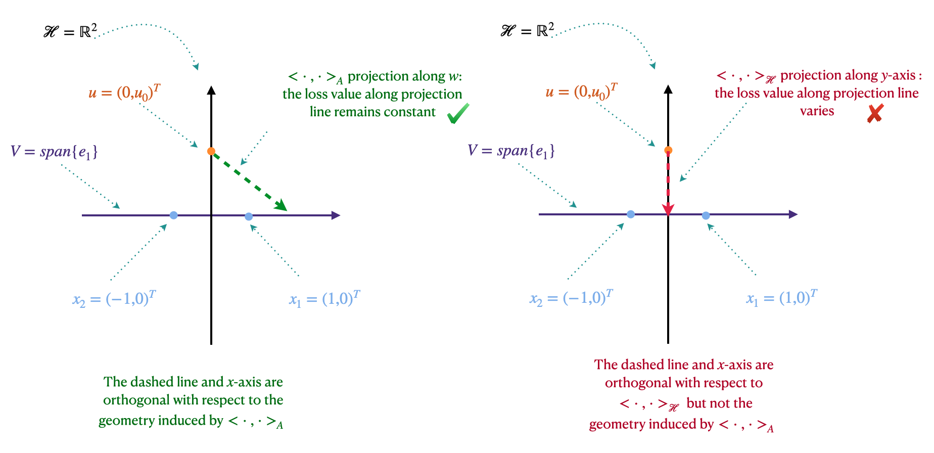
Figure 3.1. Illustration of the variation of preference loss with respect to the underlying geometry. When projecting along the $\langle\cdot,\cdot\rangle_{\mathcal{H}}$, the loss value changes along the projection line. However, when projecting along the line induced by $\langle\cdot,\cdot\rangle_{A}$, the loss remains constant. This observation highlights the significance of the underlying geometry and serves as the basis for proving the representer theorem.

The choice of the inner product on $\mathcal{H}$ play a crucial role in the validity of Theorem 3 as we formulated in Section 3.1. In this subsection, we illustrate this importance by giving an example. Consider the case $\mathcal{H}=\mathbb{R}^{2}$ with $S=\{x_{1},x_{2}\}$ for $x_{1}=e_{1}=(1,0)^{T}$ and $x_{2}=-e_{1}=(-1,0)^{T}$. In this case,

$$\mathcal{H}=\mathbb{R}^{2},$$

$$V=\operatorname*{span}\{e_{1}\}\simeq\mathbb{R}\hookrightarrow\mathbb{R}^{2}.$$

Next, let us assume that $u=(0,u_{0})^{T}$ lies on the $y$-axis. This is illustrated in Figure 3.1 . Let $A\in\mathcal{F}_{\mathcal{H}}$ has the following representation,

$$A=\begin{pmatrix}1&1\\ 1&2\end{pmatrix},$$

and denotes the metric on $\mathcal{H}$ that we would like to learn. We can think of the distance difference between $\left\|x_{1}-u\right\|_{A}^{2}-\left\|x_{2}-u\right\|_{A}^{2}$ as preference loss as its sign represents whether $u$ prefers product $x_{1}$ or $x_{2}$. We would ideally like to find an equivalent problem on $V$. We may move $u$ in such a way that the value of the loss remains unchanged. However, since in general $u$ does not lie on $V$, such transformation is not clear. Using $\langle\cdot,\cdot\rangle_{\mathcal{H}}$ one may move $u$ on the $y$ axis (i.e. Euclidean projection) and one can easily show that the loss depends on the location of $u$ on the projection line. More precisely, for $u_{t}=(0,t)^{T}$, $0\leq t\leq u_{0}$ we have,

$$\left\|x_{1}-u_{t}\right\|_{A}^{2}-\left\|x_{2}-u_{t}\right\|_{A}^{2}=-4t,$$

therefore, the difference depends on the location of the point on $y$-axis (i.e. $t$ parameter). Indeed we suggest projecting along the orthogonal line that is induced by the inner product obtained from $A$ which may not necessarily be Euclidean. Note the inner product $\langle\cdot,\cdot\rangle_{A}$ becomes,

$$\langle u,v\rangle_{A}:=v^{T}Au,$$

Now one can easily check that for $w=(1,-1)^{T}$,

$$\langle e_{1},w\rangle_{A}=0,$$

which means that the orthogonal projection with respect to geometry that is induced by $\langle\cdot,\cdot\rangle_{A}$ is in fact in the direction of $w$. Now if we consider parametrization in $w$ direction by, $u_{t}=(t,-t+u_{0})^{T}$ for $0\leq t\leq u_{0}$ then we have,

$$\left\|x_{1}-u_{t}\right\|_{A}^{2}-\left\|x_{2}-u_{t}\right\|_{A}^{2}=-4u_{0},$$

The critical aspect of the above statement is that $-4u_{0}$ remains constant regardless of the value of $t$. As a result, projecting along the geometry defined by $A$ does not alter the magnitude of the preference loss. This straightforward insight serves as the foundation for our representer theorem presented in Section 3 , as demonstrated in Figure 3.1.

4. Applications in RKHS

In Section 3, we established representer theorems for metric and preference learning in a general Hilbert space. Now, we turn our attention to the case of reproducing kernel Hilbert spaces (RKHS). Specifically, we aim to apply Theorem 3 and Theorem 4 in the context of RKHS so that we formulate problems in Euclidean spaces for practical application. To this end, we consider the setting where $\mathcal{X}=\mathbb{R}^{d}$ and $k$ is a kernel on $\mathcal{X}$. Let $\mathcal{H}_{k}$ denote the RKHS associated with $k$. Next, we assume that $S^{\prime}=\{s_{1},...,s_{m}\}\subset\mathcal{X}$ is a set of embedded items in $\mathcal{X}$. Next, using $k$, for $1\leq i\leq m$, we can associate the following in $\mathcal{H}_{k}$,

$$x_{i}:=k(s_{i},\cdot),$$

and therefore we can transform the problem into $\mathcal{H}_{k}$ as in Section 3. Now Theorem 3 and Theorem 4 apply to convert infinite dimensional optimization to finite dimensional equivalent. The following proposition finds an equivalent optimization in finite dimensional Euclidean space.

Proposition 5.

Assume

$$S=\{k(\cdot,s_{1}),...,k(\cdot,s_{m})\},$$

forms a linearly independent set. Then:

• Solutions of F and FT can be represented in terms of kernel terms as follows,

  $$A=\sum_{i,j=1}^{m}a_{ij}k(\cdot,s_{i})\otimes k(\cdot,s_{j}),$$

  $$u=\sum_{i=1}^{m}b_{i}k(\cdot,s_{i}),$$

  where in above we identified the space of linear maps on $V$ with $V\otimes V$ using $\langle\cdot,\cdot\rangle_{\mathcal{H}}$.

• Moreover, by choosing an orthonormal basis for $V$, there is a one to one correspondence between solutions of F with the solutions of the following problem in $\mathbb{R}^{m}$.

  (EF) $$\min_{A\in\mathbb{S}^{m}_{+},u\in\mathbb{R}^{m}}\sum_{i=1}^{n}\ell(\operatorname*{sign}(\left\|\alpha_{z^{i}_{1}}-u\right\|^{2}_{A}-\left\|\alpha_{z^{i}_{2}}-u\right\|^{2}_{A}),y^{i})+\lambda\left\|u\right\|_{A}^{2},$$

  and one to one correspondence between the solutions of FT with the solutions of the following problem in $\mathbb{R}^{m}$,

  (EFT) $$\min_{A\in\mathbb{S}^{m}_{+}}\sum_{i=1}^{n}\ell(\operatorname*{sign}(\left\|\alpha_{z^{i}_{1}}-\alpha_{z^{i}_{2}}\right\|^{2}_{A}-\left\|\alpha_{z^{i}_{1}}-\alpha_{z^{i}_{3}}\right\|^{2}_{A}),y^{i}),$$

  where $\mathbb{S}^{m}_{+}$ denotes space of symmetric positive definite matrices on $\mathbb{R}^{m}$ and for $u\in\mathbb{R}^{m}$ and $A\in\mathbb{S}^{m}_{+}$,

  $$\left\|u\right\|^{2}_{A}=u^{T}Au,$$

  and for $x=k(\cdot,s)\in\mathcal{H}$, $\alpha_{x}=(\alpha_{1},...,\alpha_{m})^{T}\in\mathbb{R}^{m}$ and $\alpha_{i}$ is defined by,

  $$\alpha_{i}=\frac{1}{\sqrt{D_{i-1}D_{i}}}\begin{vmatrix}k(s_{1},s_{1})&\dots&\dots&k(s_{1},s_{i})\\ \vdots&\ddots&\ddots&\vdots\\ k(s_{i-1},s_{1})&\dots&\dots&k(s_{i-1},s_{i})\\ k(s,s_{1})&\dots&\dots&k(s,s_{i})\end{vmatrix},$$

  and $D_{0}=1$ and for $1\leq i\leq m$, $D_{i}$ is defined as follows,

  $$D_{i}=\begin{vmatrix}k(s_{1},s_{1})&\dots&\dots&k(s_{1},s_{i})\\ \vdots&\ddots&\ddots&\vdots\\ k(s_{i-1},s_{1})&\dots&\dots&k(s_{i-1},s_{i})\\ k(s_{i},s_{1})&\dots&\dots&k(s_{i},s_{i})\end{vmatrix}.$$

Proof.

The first item follows from the fact that $S$ is linearly independent. The proof of the second item is a direct application of Lemma 12. ∎

Remark 6.

Note that, in practice, the computation of $\alpha_{x}$ in Proposition 5 can be carried out efficiently using the iterative form of the Gram-Schmidt process as well.

5. Proofs

In this section, we provide complete proof for the theorems introduced in the previous sections.

Lemma 6.

Let $A\in\mathcal{F}_{\mathcal{H}}$, then,

$$\langle x,y\rangle_{A}:=\langle Ax,y\rangle_{\mathcal{H}},$$

defines an inner product on $\mathcal{H}$.

Proof.

The proof easily follows from the definition. We show the details for the purpose of completeness. For $x\neq 0$, we have,

$$\langle x,x\rangle_{A}=\langle Ax,x\rangle_{\mathcal{H}}>0,$$

where we used the fact that $A$ is a positive operator. Next,

$$\langle x,y\rangle_{A}=\langle Ax,y\rangle_{\mathcal{H}}=\langle x,Ay\rangle_{\mathcal{H}}=\langle Ay,x\rangle_{\mathcal{H}}=\langle y,x\rangle_{A},$$

where we used the fact that $A$ is self-adjoint and $\langle\cdot,\cdot\rangle_{\mathcal{H}}$ is an inner product. Linearity for each coordinate follows from the fact that $A$ is a linear operator and $\langle\cdot,\cdot\rangle_{\mathcal{H}}$ is an inner product. Therefore, $\langle\cdot,\cdot\rangle_{A}$ is an inner product on $\mathcal{H}$. ∎

Lemma 7.

For $A\in\mathcal{F}_{V}$, define $B:=A\oplus\operatorname*{Id}$ by,

$$B:\mathcal{H}\to\mathcal{H}$$

$$B(h^{T}+h^{\perp}):=A(h^{T})+h^{\perp}.$$

where the following orthogonal decomposition with respect to $\langle\cdot,\cdot\rangle_{\mathcal{H}}$ is considered,

$$\mathcal{H}=V\oplus V^{\perp},$$

and $h\in\mathcal{H}$ is represented as $h=h^{T}+h^{\perp}$. Then $B$ is positive, self-adjoint, and bounded.

Proof.

It is clear from the definition that $B$ is a linear operator. To show that $B$ is positive,

$$\langle Bx,x\rangle_{\mathcal{H}}=\langle A(x^{T})+x^{\perp},x^{T}+x^{\perp}\rangle_{\mathcal{H}}=\langle A(x^{T}),x^{T}\rangle_{\mathcal{H}}+\langle x^{\perp},x^{\perp}\rangle_{\mathcal{H}}>0,$$

where we used the fact that $A$ is a positive operator and applied the Pythagorean theorem. To show that $B$ is bounded we have,

$$\langle Bx,Bx\rangle_{\mathcal{H}}=\langle A(x^{T})+x^{\perp},A(x^{T})+x^{\perp}\rangle_{\mathcal{H}}=\langle A(x^{T}),A(x^{T})\rangle_{\mathcal{H}}+\langle x^{\perp},x^{\perp}\rangle_{\mathcal{H}},$$

and boundedness follows from the fact that $A$ is bounded. To show that $B$ is self-adjoint, we have,

$$\langle Bx,y\rangle_{\mathcal{H}}=\langle A(x^{T})+x^{\perp},y\rangle_{\mathcal{H}} =\langle x^{\perp},y\rangle_{\mathcal{H}}+\langle A(x^{T}),y\rangle_{\mathcal{H}}$$

$$=\langle x^{\perp},y^{\perp}\rangle_{\mathcal{H}}+\langle x^{T},A(y^{T})\rangle_{\mathcal{H}}$$

$$=\langle x,y^{\perp}\rangle_{\mathcal{H}}+\langle x,A(y^{T})\rangle_{\mathcal{H}}$$

$$=\langle x,By\rangle_{\mathcal{H}}.$$

Thus, $B$ is positive, self-adjoint, and bounded. ∎

Proposition 8.

Let $\langle\cdot,\cdot\rangle_{A}$ be an inner product on $V\subset\mathcal{H}$, for some $A\in\mathcal{F}_{V}$. Then there exist $B\in\mathcal{F}_{\mathcal{H}}$ such that,

$$\langle\cdot,\cdot\rangle_{B}|_{V}=\langle\cdot,\cdot\rangle_{A}.$$

Conversely, suppose $\langle\cdot,\cdot\rangle_{B}$ is an inner product on $\mathcal{H}$ for some $B\in\mathcal{F}_{\mathcal{H}}$ then there exist $A\in\mathcal{F}_{V}$ such that,

$$\langle\cdot,\cdot\rangle_{B}|_{V}=\langle\cdot,\cdot\rangle_{A}.$$

Proof.

Consider the following orthogonal decomposition with respect to $\langle\cdot,\cdot\rangle_{\mathcal{H}}$,

$$\mathcal{H}=V\oplus V^{\perp}.$$

For $A\in\mathcal{F}_{V}$, define $B:=A\oplus\operatorname*{Id}$ by,

$$B:\mathcal{H}\to\mathcal{H}$$

$$B(h^{T}+h^{\perp}):=A(h^{T})+h^{\perp},$$

where $h=h^{T}+h^{\perp}$ for $h^{T}\in V$ and $h^{\perp}\in V^{\perp}$. It can be easily checked that $B$ is positive, self-adjoint, and bounded (See Lemma 7). It also follows from the definition of $B$ that,

$$B|_{V}=A,$$

therefore,

$$\langle\cdot,\cdot\rangle_{B}|_{V}=\langle\cdot,\cdot\rangle_{A}.$$

Conversely, suppose $B\in\mathcal{F}_{\mathcal{H}}$. Consider the projection operator with respect to $\langle\cdot,\cdot\rangle_{\mathcal{H}}$,

$$P:\mathcal{H}\to V,$$

and set,

$$A:V\to V$$

$$A(x)=PB(x).$$

It is clear from the definition that $A$ is bounded and linear. Next, for $x\in V$, we also have,

$$\langle Ax,x\rangle_{\mathcal{H}}=\langle PBx,x\rangle_{\mathcal{H}}=\langle Bx,x\rangle_{\mathcal{H}}>0,$$

which shows that $A$ is positive. Next, for $x,y\in V$,

$$\langle Ax,y\rangle_{\mathcal{H}}=\langle PBx,y\rangle_{\mathcal{H}}=\langle Bx,y\rangle_{\mathcal{H}}=\langle x,By\rangle_{\mathcal{H}}=\langle x,PBy\rangle_{\mathcal{H}},$$

where we used the fact that $x,y\in V$ and $B$ is self-adjoint. This shows that $A$ is self-adjoint. Next, for $x,y\in V$, we have,

$$\langle x,y\rangle_{B}=\langle Bx,y\rangle_{\mathcal{H}}=\langle PBx+(Bx)^{\perp},y\rangle_{\mathcal{H}}=\langle PBx,y\rangle_{\mathcal{H}}=\langle x,y\rangle_{A},$$

therefore we showed there is $A\in\mathcal{F}_{V}$ such that,

$$\langle\cdot,\cdot\rangle_{B}|_{V}=\langle\cdot,\cdot\rangle_{A},$$

and we are done. ∎

Proposition 9.

Let $A^{\ast}\in\mathcal{F}_{\mathcal{H}},u^{\ast}\in\mathcal{\mathcal{H}}$ be a solution to I. Equip $\mathcal{H}$ with $\langle\cdot,\cdot\rangle_{A^{\ast}}$ and let $u^{\ast}=u^{\perp}+u^{T}$ where $u^{\perp}\in V^{\perp}$ and $u^{T}\in V$. Note that the orthogonal decomposition is with respect to $\langle\cdot,\cdot\rangle_{A^{\ast}}$ and not $\langle\cdot,\cdot\rangle_{\mathcal{H}}$. Then $(A^{\ast},u^{T})$ is also a solution to I. Moreover, let $B^{\ast}\in\mathcal{F}_{V}$ denote the corresponding inner product that comes from Proposition 1,

$$\langle\cdot,\cdot\rangle_{A^{\ast}}|_{V}=\langle\cdot,\cdot\rangle_{B^{\ast}},$$

then $(B^{\ast},u^{T})$ is a solution to II. Conversely, let $(B^{\ast},u)$ be a solution to II, and let $A^{\ast}\in\mathcal{F}_{\mathcal{H}}$ be the corresponding operator from Proposition 1 that satisfies,

$$\langle\cdot,\cdot\rangle_{A^{\ast}}|_{V}=\langle\cdot,\cdot\rangle_{B^{\ast}},$$

then $(A^{\ast},u)$ is also a solution to I.

Proof.

First, note that since $V$ is finite dimensional the orthogonal decomposition with respect to $\langle\cdot,\cdot\rangle_{A^{\ast}}$ exists. Next, write,

$$u^{\ast}=u^{T}+u^{\perp},$$

For $1\leq i\leq n$, we have,

$$\ell(\operatorname*{sign}(\left\|z^{i}_{1}-u^{\ast}\right\|^{2}_{A^{\ast}}-\left\|z^{i}_{2}-u^{\ast}\right\|^{2}_{A^{\ast}}),y^{i})$$

$$= \ell(\operatorname*{sign}(\left\|z^{i}_{1}-(u^{T}+u^{\perp})\right\|^{2}_{A^{\ast}}-\left\|z^{i}_{2}-(u^{T}+u^{\perp})\right\|^{2}_{A^{\ast}}),y^{i})$$

$$= \ell(\operatorname*{sign}(\left\|(z^{i}_{1}-u^{T})-u^{\perp})\right\|^{2}_{A^{\ast}}-\left\|(z^{i}_{2}-u^{T})-u^{\perp})\right\|^{2}_{A^{\ast}}),y^{i})$$

$$= \ell(\operatorname*{sign}(\left\|(z^{i}_{1}-u^{T})\right\|^{2}_{A^{\ast}}+\left\|u^{\perp}\right\|^{2}_{A^{\ast}}-\left\|(z^{i}_{2}-u^{T})\right\|^{2}_{A^{\ast}}-\left\|u^{\perp}\right\|^{2}_{A^{\ast}}),y^{i})$$

$$= \ell(\operatorname*{sign}(\left\|(z^{i}_{1}-u^{T})\right\|^{2}_{A^{\ast}}-\left\|(z^{i}_{2}-u^{T})\right\|^{2}_{A^{\ast}}),y^{i}).$$

Above implies that,

$$\sum_{i=1}^{n}\ell(\operatorname*{sign}(\left\|z^{i}_{1}-u^{\ast}\right\|^{2}_{A^{\ast}}-\left\|z^{i}_{2}-u^{\ast}\right\|^{2}_{A^{\ast}}),y^{i})=\sum_{i=1}^{n}\ell(\operatorname*{sign}(\left\|z^{i}_{1}-u^{T}\right\|^{2}_{A^{\ast}}-\left\|z^{i}_{2}-u^{T}\right\|^{2}_{A^{\ast}}),y^{i}).$$

Therefore if $(A^{\ast},u^{\ast})$ solves I then $(A^{\ast},u^{T})$ also solves I. Now by Proposition 1, it is clear that $(B^{\ast},u^{T})$ solves II. The converse follows similarly. Let $(B^{\ast},v)$, $v\in V$ be a solution to II. Let $A^{\ast}\in\mathcal{F}_{\mathcal{H}}$ be the corresponding operator obtained by Proposition 1. We claim that $(A^{\ast},v)$ also solves I. If not, there exist $(A_{1}^{\ast},u_{1})$ with smaller loss. Then arguing as above we know that the loss for $(A_{1}^{\ast},u_{1})$ would be same as the loss for $(A_{1}^{\ast},u^{T}_{1})$ which would be same as the loss for $(B_{1}^{\ast},u^{T}_{1})$. Therefore $(B_{1}^{\ast},u^{T}_{1})$ has smaller loss that $(B^{\ast},v)$ which is a contradiction. ∎

Theorem 10 (Representer Theorem for the simultaneous metric and preference learning).

Let $\lambda>0$ and consider the following infinite dimensional regularized problem,

(R) $$\min_{A\in\mathcal{F}_{\mathcal{H}},u\in\mathcal{H}}\sum_{i=1}^{n}\ell(\operatorname*{sign}(\left\|z^{i}_{1}-u\right\|^{2}_{A}-\left\|z^{i}_{2}-u\right\|^{2}_{A}),y^{i})+\lambda\left\|u\right\|^{2}_{A},$$

and it’s finite-dimensional equivalent as follows,

(F) $$\min_{A\in\mathcal{F}_{V},u\in V}\sum_{i=1}^{n}\ell(\operatorname*{sign}(\left\|z^{i}_{1}-u\right\|^{2}_{A}-\left\|z^{i}_{2}-u\right\|^{2}_{A}),y^{i})+\lambda\left\|u\right\|^{2}_{A},$$

Let $A^{\ast}\in\mathcal{F}_{H}$ and $B^{\ast}\in\mathcal{F}_{V}$ be pairing as in Proposition 1. Then $(A^{\ast},u)$ is a solution to R iff $(B^{\ast},u)$ is a solution to F with same optimal value. In particular this forces $u\in V$.

Proof.

Let $(A^{\ast},u)$ be a solution to R. By Proposition 2, we get a smaller loss for the regularized term when we project on $V$ (with respect to $\langle\cdot,\cdot\rangle_{A^{\ast}})$ while keeping the value of the other term unchanged, therefore $u\in V$. Next, we claim that $(B^{\ast},u)$ is a solution to F. If not, there exist a solution $(B_{1},v_{1})$ with smaller loss. Let $A_{1}$ the pairing of $B_{1}$ obtained from Proposition 1. It follows that $(A_{1},v_{1})$ has a same loss value for R as $(B_{1},v_{1})$ for F. Therefore, $(A_{1},v_{1})$ has smaller loss that $(A^{\ast},u)$ which is a contradiction. The converse follows with a similar argument and we are done. ∎

5.1. The Gram-Schmidt process

In this section, we recall the determinant form of the Gram-Schmidt process. We refer to [Gan59] for detailed discussion. Let $\mathcal{H}$, equipped with $\langle\cdot,\cdot\rangle_{\mathcal{H}}$ be an inner product space.

Theorem 11 (Gram-Schmidt Determinant Formula).

Let $\{x_{1},...,x_{m}\}\in\mathcal{H}$ be linearly independent and set,

$$V=\operatorname*{span}\{x_{1},...,x_{m}\}\subset\mathcal{H}.$$

Then $\{e_{i}\}_{i=1}^{m}$ forms an orthonormal basis for $V$ where for $1\leq i\leq m$, $e_{i}$ is defined by,

$$e_{i}=\frac{1}{\sqrt{D_{i-1}D_{i}}}\begin{vmatrix}\langle x_{1},x_{1}\rangle_{\mathcal{H}}&\dots&\dots&\langle x_{1},x_{i}\rangle_{\mathcal{H}}\\ \vdots&\ddots&\ddots&\vdots\\ \langle x_{i-1},x_{1}\rangle_{\mathcal{H}}&\dots&\dots&\langle x_{i-1},x_{i}\rangle_{\mathcal{H}}\\ x_{1}&\dots&\dots&x_{i}\end{vmatrix},$$

where for each $1\leq i\leq m$, we compute a formal $i\times i$ determinant and $D_{0}=1$ and for $1\leq i\leq m$, $D_{i}$ is defined as follows,

$$D_{i}=\begin{vmatrix}\langle x_{1},x_{1}\rangle_{\mathcal{H}}&\dots&\dots&\langle x_{1},x_{i}\rangle_{\mathcal{H}}\\ \vdots&\ddots&\ddots&\vdots\\ \langle x_{i-1},x_{1}\rangle_{\mathcal{H}}&\dots&\dots&\langle x_{i-1},x_{i}\rangle_{\mathcal{H}}\\ \langle x_{i},x_{1}\rangle_{\mathcal{H}}&\dots&\dots&\langle x_{i},x_{i}\rangle_{\mathcal{H}}\end{vmatrix}.$$

Lemma 12.

Consider the same setting as in Theorem 11 and let $x\in\mathcal{H}$ and write $x=x^{T}+x^{\perp}$ where the decomposition is with respect to $\langle\cdot,\cdot\rangle_{\mathcal{H}}$. Then $x^{T}$ can be represented by $\alpha_{x}=(\alpha_{1},...,\alpha_{m})^{T}\in\mathbb{R}^{m}$ as follows,

$$x^{T}=\sum_{i=1}^{m}\langle x,e_{i}\rangle_{\mathcal{H}}e_{i}=\sum_{i=1}^{m}\alpha_{i}e_{i},$$

and $\alpha_{i}$ is defined by,

$$\alpha_{i}=\frac{1}{\sqrt{D_{i-1}D_{i}}}\begin{vmatrix}\langle x_{1},x_{1}\rangle_{\mathcal{H}}&\dots&\dots&\langle x_{1},x_{i}\rangle_{\mathcal{H}}\\ \vdots&\ddots&\ddots&\vdots\\ \langle x_{i-1},x_{1}\rangle_{\mathcal{H}}&\dots&\dots&\langle x_{i-1},x_{i}\rangle_{\mathcal{H}}\\ \langle x,x_{1}\rangle_{\mathcal{H}}&\dots&\dots&\langle x,x_{i}\rangle_{\mathcal{H}}\end{vmatrix}.$$

Proof.

This simply follows from Leibniz formula for determinants applying to $e_{i}$ obtaining from Theorem 11. ∎

References

- [BHS13] Aurélien Bellet, Amaury Habrard, and Marc Sebban, A survey on metric learning for feature vectors and structured data, arXiv preprint arXiv:1306.6709 (2013).
- [CKTK10] Ratthachat Chatpatanasiri, Teesid Korsrilabutr, Pasakorn Tangchanachaianan, and Boonserm Kijsirikul, A new kernelization framework for mahalanobis distance learning algorithms, Neurocomputing 73 (2010), no. 10-12, 1570–1579.
- [FH10] Johannes Fürnkranz and Eyke Hüllermeier, Preference learning and ranking by pairwise comparison, Preference learning, Springer, 2010, pp. 65–82.
- [Gan59] Feliks R Gantmacher, The theory of matrices, Co., New York 2 (1959).
- [HYC+17] Cheng-Kang Hsieh, Longqi Yang, Yin Cui, Tsung-Yi Lin, Serge Belongie, and Deborah Estrin, Collaborative metric learning, Proceedings of the 26th international conference on world wide web, 2017, pp. 193–201.
- [JN11] Kevin G Jamieson and Robert Nowak, Active ranking using pairwise comparisons, Advances in neural information processing systems 24 (2011).
- [K+13] Brian Kulis et al., Metric learning: A survey, Foundations and Trends® in Machine Learning 5 (2013), no. 4, 287–364.
- [KvL17] Matthäus Kleindessner and Ulrike von Luxburg, Kernel functions based on triplet comparisons, Advances in neural information processing systems 30 (2017).
- [KW71] George Kimeldorf and Grace Wahba, Some results on tchebycheffian spline functions, Journal of mathematical analysis and applications 33 (1971), no. 1, 82–95.
- [Mah36] Prasanta Chandra Mahalanobis, On the generalized distance in statistics, National Institute of Science of India, 1936.
- [SHS01] Bernhard Schölkopf, Ralf Herbrich, and Alex J Smola, A generalized representer theorem, Computational Learning Theory: 14th Annual Conference on Computational Learning Theory, COLT 2001 and 5th European Conference on Computational Learning Theory, EuroCOLT 2001 Amsterdam, The Netherlands, July 16–19, 2001 Proceedings 14, Springer, 2001, pp. 416–426.
- [Wah90] Grace Wahba, Spline models for observational data, SIAM, 1990.
- [XD20] Austin Xu and Mark Davenport, Simultaneous preference and metric learning from paired comparisons, Advances in Neural Information Processing Systems 33 (2020), 454–465.