Sorta Solving the OPF by Not Solving the OPF:
DAE Control Theory and the Price of Realtime Regulation

Abstract

This paper presents a new approach to solve or approximate the AC optimal power flow (ACOPF). By eliminating the need to solve the ACOPF every few minutes, the paper showcases how a realtime feedback controller can be utilized in lieu of ACOPF and its variants. By (i) forming the grid dynamics as a system of differential algebraic equations (DAE) that naturally encode the non-convex OPF power flow constraints, (ii) utilizing advanced DAE-Lyapunov theory, and (iii) designing a feedback controller that captures realtime uncertainty while being uncertainty-unaware, the presented approach demonstrates promises of obtaining solutions that are close to the OPF ones without needing to solve the OPF. The proposed controller responds in realtime to deviations in renewables generation and loads, guaranteeing transient stability, while always yielding feasible solutions of the ACOPF with no constraint violations. As the studied approach herein indeed yields slightly more expensive realtime generator controls, the corresponding price of realtime control and regulation is examined. Cost-comparisons with the traditional ACOPF are also showcased—all via case studies on standard power networks.

I Introduction and Paper Contributions

IT is not an overstatement that the OPF problem—and its many variants—is arguably the most researched and solved optimization problem in the world. OPF [1] refers to computing setpoints of generators in a power network every few minutes, allowing generation to meet the varying demand. In short, the problem minimizes the cost of generation from mostly fossil fuel-based power plants subject to power balance in transmission power lines (acting as equality constraints or $\bm{h}(\bm{x})=\bm{0}$) and thermal line, voltages and generation limits (acting as inequality constraints or $\bm{g}(\bm{x})\leq\bm{0}$). This optimization problem can be written as

$$\textbf{OPF:}\;\;\;\;\;\;\operatorname*{minimize}\;\;\;\;\;f(\bm{x})\;\;\;\operatorname*{subject\ to}\;\;\;\;\;\;\bm{g}(\bm{x})\leq\bm{0}\;\;,\;\;\bm{h}(\bm{x})=\bm{0}.$$ (1)

Due to the nonconvexity in the power balance equality constraints $\bm{h}(\bm{x})=\bm{0}$, the OPF is infamously non-convex. The infamy is not because the nonconvexity is too insufferable however insufferability is defined; it is because OPF has become a textbook example of practical optimization problems in operations research and systems engineering.

Brief Literature Review. In pursuit of overcoming this nonconvexity, hundreds of papers yearly investigate methods to solve variants of OPF. The OPF can also make you a millionaire: The US department of energy and ARPA-E have a competition, called grid optimization (GO) Competition [2, 3], where academics and practitioners compete in solving variants of the OPF with up to $3 million in prizes. To solve the OPF, academics often resort to one of these four approaches. (i) Assume DC power flow and eliminate some variables, resulting in convex quadratic programs that can be solved efficiently for large power systems [4, 5, 6, 7]. (ii) Derive semidefinite programming (SDP) relaxations of OPF appended with methods to recover an optimal solution [8, 9, 10, 11, 12, 13, 14, 15]. (iii) Design global optimization methods with some performance guarantees under various relaxations of nonconvex OPF [16, 17, 18]. (iv) Obtain machine learning-based algorithms that learn solutions to OPF [19, 20, 21, 22, 23, 24]. A thorough description of the inveterate OPF literature is outside the scope of this work.

In reality, all of the aforementioned approaches still try to actually solve (1) or its derivatives, approximations, relaxations, or restrictions. Relevant to these approaches that only focus on OPF are methods and algorithms that study stability-constrained OPF where dynamic stability or optimal control metrics are appended to the OPF [25, 26, 27, 28], thereby resulting in the integration of the two time-scales of operation (i.e., OPF) and realtime stability and control (or secondary control algorithms). Merging the two time-scales results in OPF generator setpoints that are control-aware, meaning the five-minute-setpoints allow the system to be more controllable or more stable. This, however, does not circumvent the issues with the nonconvex equality constraints in the OPF. Although seemingly orthogonal to this discussion, this pursuit of stability or control-constrained-OPF is somewhat relevant to what we propose herein.

Furthermore, due to the increasing penetration of renewable energy resources, complex load demands, and other power electronics based devices in the future power grid, the 5–10 minutes setpoints provided by the traditional OPF may not be valid/optimal because of the time-separation and slow update process [29]. With that in mind, this paper investigates a new approach of solving the OPF problem in realtime. This is done in a way by virtually ignoring (1) and dumping the OPF problem into a feedback control problem that inherently satisfies the constraint set in (1), while simultaneously performing other tasks such as load frequency regulation and realtime control. Next, we explain in detail how this approach works. More detailed discussion of the literature is omitted from here (for brevity and clarity) and instead is given after the formulation of the proposed controller (Section IV).

Main Idea. First, formulate a dynamic, differential algebraic equation (DAE) model of power systems. This model incorporates algebraic equations that model power flows (the nonconvex constraints in (1)) as well as generator dynamics. Then, solve a control problem that computes (a) OPF setpoints (i.e., generator output power) and (b) their deviations in a feedback fashion by utilizing PMU data in realtime, while forgoing the need to solve for the power flow variables—yet still somehow insuring that physical constraints are not violated. By formulating a realtime, feedback-driven control problem that solves for a time-invariant feedback gain matrix, and feeding that gain into a highly scalable differential algebraic equation (DAE) solver, we avoid actually having to solve a nonconvex optimization problem for the OPF variables.

In short, by dumping the OPF problem on a realtime, feedback controller, we kinda solve the OPF by not solving the OPF. This approach, in reality, does not actually solve the OPF with the generator’s cost curves—but as observed later in the paper, we showcase how the proposed approach is not terribly far from optimality. In a real-world setting, the DAE solver is replaced with the actual system meaning that even the DAEs do not have to be simulated. The DAEs already encode the nonconvex constraints in OPF—a key factor in the proposed approach.

Paper Contributions. The presented approach in this paper is endowed with the following key properties and contributions. The OPF-controller: (i) Circumvents the need to solve or deal with the nonconvex equality constraints modeling power flow. That is, we find generators’ setpoints in realtime while knowing that these setpoints do satisfy and abide by the power flow constraints. (ii) Deals with the uncertainty in renewables, loads, and parameters in a control-theoretic way. In contrast with vintage robust optimization or the more intricate distributionally robust optimization algorithms, the developed approach here is distribution-free and is not inherently conservative. (iii) Utilizes realtime information from grid sensors such as phasor measurement units (PMU) via state estimators allowing for realtime micro-adjustments of dispatchable generation. This is in contrast with OPF formulations that do not utilize grid measurements for better dispatch of generators. (iv) Eliminates the need to separate the OPF and the secondary control time-scales: this approach serves the purposes of both OPF and control, so the need to separate the two becomes obsolete at worst, and questionable at best. (v) Seamlessly models advanced models of renewables, resulting in setpoints for fuel-based generators that are aware of the dynamics of solar and wind farms, for example.

Notations. Bold lowercase and uppercase letters represent vectors and matrices respectively, while all calligraphic letters denotes sets such as $\mathcal{R}$, $\mathcal{N}$ etc. The set of real-valued $x$ by $y$ matrices is represented as $\mathbb{R}^{x\times y}$. Similarly positive definite matrix of size $x$ by $y$ is denoted as $\mathbb{S}_{++}^{x\times y}$. Also, we represent identity and zero matrix of appropriate dimension as $\bm{I}$ and $\bm{O}$. For any matrix $\bm{A}$, symbols $\bm{A}^{\perp}$, $\bm{A}^{T}$, $\|\bm{A}\|_{0}$, $\bar{\sigma}[\bm{A}]$, and $\|\bm{A}\|_{2}$ denote its, orthogonal complement, transpose, total number of non-zero elements, largest singular value, and $\mathcal{L}_{2}$-norm respectively. We represent positive/negative definiteness as $\succ 0$/$\prec 0$ and positive semi-definiteness by $\succeq 0$. Symbol $*$ represent the symmetric elements in a given symmetric matrix. We denote union (combination) of two set via symbol $\cup$ such as $\mathcal{G}\cup\mathcal{R}$. We use $\mathrm{diag}$ to show a diagonal matrix. The set $\mathbb{R}^{x}$ represent a column vector of $x$ elements and $\mathbb{R}_{++}$ represent a positive scalar. Given a vector $a(t)$ in time interval $t\in[0,\infty)$, its $\mathcal{L}_{2}$-norm is represented as $\sqrt{\int_{0}^{\infty}\|a(t)\|^{2}dt}$. Also, for sake of simplicity we omit time dependency, i.e., $(t)$ in representing some of the time-dependent vectors.

Paper Organization.The remainder of the paper is organized as follows: Section II summarizes the ACOPF problem formulation. Section III present the multi-machine NDAE model of power networks. Section IV explain the proposed methodology and its mathematical derivation. Numerical case studies are performed in Section V while the paper is concluded in Section VI.

II ACOPF Formulation

In this section, we briefly present the ACOPF formulation. We consider a power network consisting $N$ number of buses, modeled by a graph $(\mathcal{N},\mathcal{E})$ where $\mathcal{N}$ is the set of nodes and $\mathcal{E}$ is the set of edges. Note that $\mathcal{N}$ consists of traditional synchronous generator, renewable energy resources, and load buses, i.e., $\mathcal{N}=\mathcal{G}\cup\mathcal{R}\cup\mathcal{L}$ where $\mathcal{G}$ collects $G$ generator buses, $\mathcal{R}$ collects the buses containing $R$ renewables, while $\mathcal{L}$ collects $L$ load buses. The generator’s supplied (real and reactive) power is denoted by $(P_{\mathrm{G}i},Q_{\mathrm{G}i})$ for bus $i\in\mathcal{G}$, and the bus voltages are depicted as $v_{i}$. The bus angle is represented as $\theta_{i}$ and the angle difference in a line is $\theta_{ij}:=\theta_{i}-\theta_{j}$. The parameters $(G_{ij},B_{ij})$ respectively denote the conductance and susceptance between bus $i$ and $j$ which can be directly obtained from the network’s bus admittance matrix [30]. Furthermore, quantities $(P_{\mathrm{R}i},Q_{\mathrm{R}i})$ denote the active and reactive power generated by renewables for bus $i\in\mathcal{R}$, while $(P_{\mathrm{L}i},Q_{\mathrm{L}i})$ denote the active and reactive power consumed by the loads for bus $i\in\mathcal{L}$. Essentially, renewables are modeled as negative loads. If a bus does not have generation, load, or a renewable source attached to it, the corresponding active/reactive powers are equal to zero.

Given the above notation, the ACOPF can be written as [4]

$$\min_{\bm{P}_{\mathrm{G}},\bm{Q}_{\mathrm{G}},\bm{\theta},\bm{v}} J_{\mathrm{OPF}}(\bm{P}_{\mathrm{G}})=\sum_{i\in\mathcal{G}}a_{i}P_{\mathrm{G}i}^{2}+b_{i}P_{\mathrm{G}i}+c_{i}$$ (2a)

$$\operatorname*{subject\ to} \forall i\in\mathcal{N}:P_{\mathrm{G}i}+P_{\mathrm{R}i}+P_{\mathrm{L}i}=$$ (2h)

$$v_{i}\sum_{j=1}^{N}v_{j}\left(G_{ij}\cos\theta_{ij}+B_{ij}\sin\theta_{ij}\right)$$

$$\forall i\in\mathcal{N}:Q_{\mathrm{G}i}+Q_{\mathrm{R}i}+Q_{\mathrm{L}i}=$$

$$v_{i}\sum_{j=1}^{N}v_{j}\left(G_{ij}\sin\theta_{ij}-B_{ij}\cos\theta_{ij}\right)$$

$$\forall i\in\mathcal{G}:P_{\mathrm{G}i}^{\min}\leq P_{\mathrm{G}i}\leq P_{\mathrm{G}i}^{\max}$$

$$\forall i\in\mathcal{G}:Q_{\mathrm{G}i}^{\min}\leq Q_{\mathrm{G}i}\leq Q_{\mathrm{G}i}^{\max}$$

$$\forall i\in\mathcal{N}:v_{i}^{\min}\leq v_{i}\leq v_{i}^{\max}$$

$$\forall i\in\mathcal{N}:S_{f_{i}}\leq F_{\mathrm{max}}$$

$$\forall i\in\mathcal{N}:S_{t_{i}}\leq F_{\mathrm{max}}.$$

The variables in the ACOPF are the active/reactive powers for generator buses and angles and voltages for all buses $(\bm{P}_{\mathrm{G}},\bm{Q}_{\mathrm{G}},\bm{\theta},\bm{v})$. In (2), the objective function $J_{\mathrm{OPF}}(\bm{P}_{\mathrm{G}})$ minimizes the generator’s convex quadratic cost function with parameters $a_{i},b_{i},$ and $c_{i}$. The first two constraints model power flow balance in the network—a nonlinear, non-convex relation between the variables. The last five constraints represent upper and lower bounds on the generators’ power as well as bus voltages and line flow constraints, with $S_{f_{i}}$, $S_{t_{i}}$ representing from and to line flows and $F_{\mathrm{max}}$ denoting maximum rating of the transmission lines.

The ACOPF is usually solved every 5–10 minutes, although the frequency at which its solved depends on the computational power and updated predictions of renewables and loads. Ideally, a system operator would have all of the constraints satisfied at each time step $t$, and one would solve a realtime ACOPF that satisfies all constraints while optimizing the cost function.

In the next section, we present the dynamics of the same power system with a focus on the realtime control problem. We then showcase that the proposed realtime controller inherently satisfies some of the key ACOPF constraints.

III Dynamics of Multi-Machine Power Systems

Here, we describe the transient dynamics of a power system which by definition encode the algebraic constraints (2h) and (2h). For the same power network, we can write the 4-order dynamics of synchronous generators as [30]:

$$\dot{\delta}_{i} =\omega_{i}-\omega_{0}$$ (3a)

$$\begin{split}M_{i}\dot{\omega}_{i}&=T_{\mathrm{M}i}-P_{\mathrm{G}i}-D_{i}(\omega_{i}-\omega_{0})\end{split}$$ (3b)

$$T^{\prime}_{\mathrm{d0}i}\dot{E}^{\prime}_{i} =-\tfrac{x_{\mathrm{d}i}}{x^{\prime}_{\mathrm{d}i}}E^{\prime}_{i}+\tfrac{x_{\mathrm{d}i}-x^{\prime}_{\mathrm{d}i}}{x^{\prime}_{\mathrm{d}i}}v_{i}\cos(\delta_{i}-\theta_{i})+E_{\mathrm{fd}i}$$ (3c)

$$T_{\mathrm{CH}i}\dot{T}_{Mi} =-T_{\mathrm{M}i}-\tfrac{1}{R_{\mathrm{D}i}}(\omega_{i}-\omega_{0})+T_{\mathrm{r}i}$$ (3d)

where $\delta_{i}$, $\omega_{i}$, $E^{\prime}_{i}$, $T_{\mathrm{M}i}$ are generator’s internal states and $E_{\mathrm{fd}i}$, $T_{\mathrm{r}i}$ are generator’s controllable inputs (exciter field voltage and torque setpoint). The constant terms in (3) are as follows: $M_{i}$ is the rotor’s inertia constant ($\mathrm{pu}\times\mathrm{s}^{2}$), $D_{i}$ is the damping coefficient ($\mathrm{pu}\times\mathrm{s}$), $x_{di}$ is the direct-axis synchronous reactance ($\mathrm{pu}$), $x^{\prime}_{\mathrm{d}i}$ is the direct-axis transient reactance ($\mathrm{pu}$), $T^{\prime}_{\mathrm{d0}i}$ is the direct-axis open-circuit time constant ($\mathrm{s}$), $T_{\mathrm{CH}i}$ is the chest valve time constant, $R_{\mathrm{D}i}$ is the regulation constant for the speed-governing mechanism, and $\omega_{0}$ denotes the rotor’s synchronous speed ($\mathrm{rad/s}$). The mathematical model relating generator’s internal states $(\delta_{i},\omega_{i},E^{\prime}_{i},T_{\mathrm{M}i})$, generator’s supplied power $(P_{\mathrm{G}i},Q_{\mathrm{G}i})$, and terminal voltage ${v}_{i}$ is given by the generator’s internal algebraic constraint [30]

$$\begin{split}P_{\mathrm{G}i}&=\tfrac{1}{x^{\prime}_{\mathrm{d}i}}E^{\prime}_{i}v_{i}\sin(\delta_{i}-\theta_{i})-\tfrac{x_{\mathrm{q}i}-x^{\prime}_{\mathrm{d}i}}{2x^{\prime}_{\mathrm{d}i}x_{\mathrm{q}i}}v_{i}^{2}\sin(2(\delta_{i}-\theta_{i}))\end{split}$$ (4a)

$$\begin{split}Q_{\mathrm{G}i}&=\tfrac{1}{x^{\prime}_{\mathrm{d}i}}E^{\prime}_{i}v_{i}\cos(\delta_{i}-\theta_{i})-\tfrac{x^{\prime}_{\mathrm{d}i}+x_{\mathrm{q}i}}{2x^{\prime}_{\mathrm{d}i}x_{\mathrm{q}i}}v_{i}^{2}\\ &\quad-\tfrac{x_{\mathrm{q}i}-x^{\prime}_{\mathrm{d}i}}{2x^{\prime}_{\mathrm{d}i}x_{\mathrm{q}i}}v_{i}^{2}\cos(2(\delta_{i}-\theta_{i})).\end{split}$$ (4b)

The power flow equations, for all buses $i\in\mathcal{N}$, representing the distribution of real and reactive power are given by (2h) and (2h), which are present in the ACOPF formulation. Hence, the power flow constraints and the generator’s algebraic constraints essentially couple the rapidly varying dynamic states and control variables with the ACOPF ones.

In order to construct the nonlinear state-space representation of the multi-machine power networks (2h), (2h), (3), and (4), define ${\bm{x}}_{d}$ as the vector populating all dynamic states of the network such that ${\bm{x}}_{d}:=\begin{bmatrix}\bm{\delta}^{\top}\;\;\bm{\omega}^{\top}\;\;\bm{E}^{\prime\top}\;\;\bm{T}_{\mathrm{M}}^{\top}\end{bmatrix}^{\top}$ in which ${\bm{\delta}}:=\{\delta_{i}\}_{i\in\mathcal{G}}$, ${\bm{\omega}}:=\{\omega_{i}\}_{i\in\mathcal{G}}$, ${\bm{E}^{\prime}}:=\{E^{\prime}_{i}\}_{i\in\mathcal{G}}$, ${\bm{T}_{\mathrm{M}}}:=\{T_{\mathrm{M}i}\}_{i\in\mathcal{G}}$. Furthermore, we can define the vector of algebraic states (that overlap with some ACOPF variables) as $\bm{x}_{a}:=\begin{bmatrix}\bm{P}_{\mathrm{G}}^{\top}\;\;\bm{Q}_{\mathrm{G}}^{\top}\;\;\bm{v}^{\top}\;\;\bm{\theta}^{\top}\end{bmatrix}^{\top}$. The controllable input of the power network is defined as ${\bm{u}}:=\begin{bmatrix}\bm{E}_{\mathrm{fd}}^{\top}\;\;\bm{T}_{\mathrm{r}}^{\top}\end{bmatrix}^{\top}$ where ${\bm{E}_{\mathrm{fd}}}:=\{E_{\mathrm{fd}i}\}_{i\in\mathcal{G}}$ and ${\bm{T}_{\mathrm{r}}}:=\{T_{\mathrm{r}i}\}_{i\in\mathcal{G}}$. In addition, define the vector ${\bm{w}}$ as ${\bm{w}}:=\begin{bmatrix}\bm{P}_{\mathrm{R}}^{\top}\;\;\bm{Q}_{\mathrm{R}}^{\top}\;\;\bm{P}_{\mathrm{L}}^{\top}\;\;\bm{Q}_{\mathrm{L}}^{\top}\end{bmatrix}^{\top}$ where ${\bm{P}_{\mathrm{R}}}:=\{P_{\mathrm{R}i}\}_{i\in\mathcal{R}}$, ${\bm{Q}_{\mathrm{R}}}:=\{Q_{\mathrm{R}i}\}_{i\in\mathcal{R}}$, ${\bm{P}_{\mathrm{L}}}:=\{P_{\mathrm{L}i}\}_{i\in\mathcal{L}}$, ${\bm{Q}_{\mathrm{L}}}:=\{Q_{\mathrm{L}i}\}_{i\in\mathcal{L}}$. Essentially, vector $\bm{w}$ lumps all uncertain quantities from renewables and loads. The above notations allow us to have a compact, nonlinear differential algebraic equation (NDAE) state space model:

Dynamics: $$\dot{{\bm{x}}}_{d} ={\bm{A}}_{d}{\bm{x}}_{d}+{\bm{f}}_{d}\left({\bm{x}}_{d},{\bm{x}}_{a}\right)+\bm{B}_{d}\bm{u}$$ (5a)

Constraints: $$\bm{0} ={\bm{A}}_{a}{\bm{x}}_{a}+{\bm{f}}_{a}\left({\bm{x}}_{d},{\bm{x}}_{a}\right)+{\bm{B}}_{a}{\bm{w}}$$ (5b)

where $\bm{x}_{d}\in\mathbb{R}^{n_{d}}$, $\bm{x}_{a}\in\mathbb{R}^{n_{a}}$, $\bm{u}\in\mathbb{R}^{n_{u}}$, and $\bm{w}\in\mathbb{R}^{n_{w}}$. The functions $\bm{f}_{d}:\mathbb{R}^{n_{d}}\times\mathbb{R}^{n_{a}}\rightarrow\mathbb{R}^{n_{d}}$ and $\bm{f}_{a}:\mathbb{R}^{n_{d}}\times\mathbb{R}^{n_{a}}\rightarrow\mathbb{R}^{n_{a}}$ defined the vector-valued mapping containing the nonlinearity of generator dynamics as well as the power flow nonlinearity/nonconvexity. Matrices ${\bm{A}}_{d}\in\mathbb{R}^{n_{d}\times n_{d}}$, ${\bm{A}}_{a}\in\mathbb{R}^{n_{a}\times n_{a}}$, ${\bm{B}}_{d}\in\mathbb{R}^{n_{d}\times n_{d}}$, and ${\bm{B}}_{a}\in\mathbb{R}^{n_{a}\times n_{a}}$ define the linear portion of the dynamics and algebraic constraints. By defining $\bm{x}=\begin{bmatrix}\bm{x}_{d}&\bm{x}_{a}\end{bmatrix}^{\top}\in\mathbb{R}^{n_{x}}$ and $\bm{f}(\bm{x})=\begin{bmatrix}\bm{f}_{d}(\bm{x}_{d},\bm{x}_{a})&\bm{f}_{a}(\bm{x}_{d},\bm{x}_{a})\end{bmatrix}^{\top}$ the model (5) can also be rewritten as follows:

$$\bm{E}\dot{{\bm{x}}} ={\bm{A}}{\bm{x}}+{\bm{f}}\left({\bm{x}}\right)+{\bm{B}}{\bm{u}}+{\bm{B}}_{w}\bm{w}.$$ (6)

Having defined the NDAE power network dynamics, we note the following. (i) Herein, we showcase a fourth order generator model (i.e., each generator is modeled via four states) but this can be extended to higher order generator dynamics as well as dynamic models of solar and wind. (ii) In addition to modeling the algebraic constraints encoding lossy power flows, the presented NDAE formulation also accounts for the stator’s algebraic equation which is usually missing from ACOPF formulation. (iii) The controllable variable in the ACOPF formulation, namely $\bm{P}_{\mathrm{G}}$, is present in the dynamical system model as an algebraic variable that is controlled explicitly via $\bm{u}(t)$. This entails the following. Solving a feedback control problem that generates realtime sequence $\bm{u}(t)$ and subsequently extracting the ACOPF’s algebraic variables $\bm{x}_{a}(t)$, while satisfying the ACOPF constraints and being close to its optimal solution $J_{\mathrm{OPF}}(\bm{P}_{\mathrm{G}})$, could be specifically useful.

IV Solving OPF via DAE Control Theory

We focus now on the control problem for the NDAE model (5), which when solved will essentially solve a version of the ACOPF (2). This control problem can simply be defined as computing a constant gain matrix that can be used with the control input $\bm{u}(t)$ in a closed-loop fashion (via realtime state/output information) such that it can drive the system back to a stable equilibrium after a large disturbance. With that in mind, let us define the closed-loop system dynamics as follows:

$$\bm{E}\dot{{\bm{x}}} ={\bm{A}}{\bm{x}}+{\bm{f}}\left({\bm{x}}\right)+{\bm{B}}{\bm{u}_{C}}+{\bm{B}}_{w}\bm{w}$$ (7)

where $\bm{u}_{C}$ is the closed-loop control input and is defined as:

$$\boxed{{\bm{u}}_{{C}}:=\bm{u}_{{C}}(t)=\bm{u}_{\mathrm{ref}}^{k}+\bm{K}\left({\bm{x}}(t)-\bm{x}^{k}\right)}$$ (8)

in which $\bm{u}_{\mathrm{ref}}$ is the reference or baseline setting for the control input $\bm{u}$, $\bm{x}^{k}$ is the dynamic states information at previous time step $k$, and $\bm{K}$ is the constant controller gain matrix. The key idea is to design $\bm{K}$ such that using realtime state feedback information $\bm{x}(t)$, the closed-loop control input $\bm{u}_{C}$ can make the system robust and transiently stable against disturbances.

To that end, notice that, if we can compute $\bm{K}$ in a way such that it encodes (5b) also along with (5a) (meaning determining $\bm{K}$ for the whole NDAE system instead of eliminating (5b) and converting it to an ODE system), then the determined feedback controller $\bm{K}$ will inherently satisfy the key constraints appearing in the OPF formulation (2). This is because Eq. (5b) includes power balance equations (2h), (2h) of ACOPF and generators stator algebraic constraints (4a),(4b) which indirectly encode the constraints (2h),(2h) of the ACOPF. As for the other constraints such as limits on generators’ capacities, these can be encoded via saturation dynamics in the differential equations. Admittedly, other constraints such as thermal limits of lines cannot be modeled in this approach, and to that end we thoroughly investigate any constrained violations incurred in Section V.

With that in mind, we name the computation of such feedback controller gain $\bm{K}$ which includes (5b) in its control architecture as control-OPF feedback controller design. This is because such $\bm{K}$ ensures system transient stability after a large disturbance and also fully abides by the key OPF constraints as discussed above. To that end, we present the following results to compute such $\bm{K}$ which is based on Lyapunov stability theory as follows:

$$\small{\textsc{({Control-OPF})}}\operatorname*{minimize}_{\bm{F},\bm{S},\bm{X},{\lambda},\epsilon,\mu,\kappa} \;\;\;a_{1}\lambda+a_{2}\mu+a_{3}\epsilon_{1}+a_{4}\epsilon_{2}$$

$$\operatorname*{subject\ to} \;\;\;\mathrm{LMI}\;\eqref{eq:LMI_Hinf},\;\mathrm{LMIs}\;\eqref{eq:LMIs_size},$$

$$\;\;\;\lambda\bm{I}-\bm{X}^{\top}\bm{E}\bm{X}\succ 0,$$

$$\;\;\;\bm{X}\succ 0,\lambda>0,\gamma>0,$$

$$\;\;\;\epsilon_{1}>0,\epsilon_{2}>0,\kappa>0\vspace{-0.6cm}$$

where

• $a_{1}$, $a_{2}$, $a_{3}$, and $a_{4}$ are known weighting constants.

• The variables in control-OPF are matrices $\bm{S}\in\mathbb{R}^{n_{a}\times n_{x}}$, $\bm{F}\in\mathbb{R}^{n_{u}\times n_{x}}$, $\bm{X}\in\mathbb{S}_{++}^{n_{x}\times n_{x}}$, and scalars $\lambda,\mu,\kappa,\epsilon_{1},\epsilon_{2}\in\mathbb{R}_{++}$.

• LMI (9) is defined as

  $$\begin{bmatrix}\bm{T}^{\top}\bm{A}^{\top}_{c}+\bm{A}_{c}\bm{T}&\bm{B}_{w}&\bm{I}&\bm{T}^{\top}\bm{\Phi}^{\top}&\kappa\alpha\bm{T}^{\top}\\ \bm{B}_{w}^{\top}&-\mu\bm{I}&\bm{O}&\bm{D}_{w}^{\top}&\bm{O}\\ \bm{I}&\bm{O}&-\kappa\bm{I}&\bm{O}&\bm{O}\\ \bm{\Phi}\bm{T}&\bm{D}_{w}&\bm{O}&-\bm{I}&\bm{O}\\ \kappa\alpha\bm{T}&\bm{O}&\bm{O}&\bm{O}&-\bm{I}\end{bmatrix}\prec 0$$ (9)

  where $\bm{T}=\bm{X}\bm{E}^{\top}+\bm{E}^{\perp}\bm{S}$ and $\bm{E}^{\perp}\in\mathbb{R}^{n_{x}\times n_{a}}$ represent the orthogonal complement of matrix $\bm{E}$.

• LMIs (10) are defined as:

  $$\begin{bmatrix}-\epsilon_{1}\bm{I}&\bm{F}^{\top}\\ \bm{F}&-\bm{I}\end{bmatrix}\prec 0,\,\,\,\,\,\begin{bmatrix}-\epsilon_{2}\bm{I}&\bm{I}\\ \bm{I}&-\bm{T}-\bm{T}^{\top}\end{bmatrix}\prec 0$$ (10)

• The corresponding controller gain matrix $\bm{K}$ can be obtained as

  $$\bm{K}=\bm{F}\bm{T}^{-1}$$ (11)

• The designed control-OPF is a convex semi-definite optimization problem and thus can easily be solved via various optimization solvers.

In the following sequel we present the detailed explanation of each variables and the mathematical derivation of the proposed control-OPF formulation.

IV-A Mathematical Derivation of Control-OPF

To begin with, let us assume there is an unknown disturbance in the system and the new value of the vector $\bm{w}$ is $\bm{w}^{\prime}$. This disturbance will move the states of the power network from its initial equilibrium to a new equilibrium $\bm{x}^{\prime}$. With that in mind, the perturbed closed loop dynamics i.e $\Delta\bm{x}=\bm{x}-\bm{x}^{\prime}$ of (7) can be written as:

$$\bm{E}\Delta\dot{\bm{x}} =(\bm{A}+\bm{BK})\Delta\bm{x}+\Delta\bm{f}(\Delta\bm{x})+\bm{B}_{w}\Delta\bm{w}.$$ (12)

Now the main idea is to design in $\bm{K}$ such that the perturbed dynamics (12) converge asymptotically to zero. Which in other words means the design $\bm{K}$ guarantees that the system dynamics stabilize at the new equilibrium after a large disturbance. With that in mind, to compute such controller gain matrix $\bm{K}$ we utilize the robust $\mathcal{H}_{\infty}$ notion [31]. The core idea in $\mathcal{H}_{\infty}$-based controller design is that the controller makes sure that the norm of the performance index is always less than constant times the norm of disturbance i.e $\left\lVert\bm{z}_{1}\right\rVert^{2}_{\mathcal{L}_{2}}<\gamma^{2}\left\lVert{\bm{w}}\right\rVert^{2}_{\mathcal{L}_{2}}$, where $\bm{z}$ is the user-defined performance index and $\gamma$ is optimization variable commonly known as performance level in the control theocratic literature. To that end, let us consider the performance index for the perturbed closed loop system (12) to be: $\Delta\bm{z}_{1}=\bm{C}\Delta\bm{x}+\bm{D}\Delta\bm{u}+\bm{D}_{w}\Delta\bm{w}\in\mathbb{R}^{n_{x}}$ which can also be written as: $\Delta\bm{z}_{1}=(\bm{C}+\bm{DK})\Delta\bm{x}+\bm{D}_{w}\Delta\bm{w}$, where the matrices $\bm{C}\in\mathbb{R}^{n_{x}\times n_{x}}$, $\bm{D}\in\mathbb{R}^{n_{x}\times n_{u}}$, and $\bm{D}_{w}\in\mathbb{R}^{n_{x}\times n_{w}}$ are user-defined penalizing matrices (meaning how much weight should be given to each states and control inputs in response to the disturbance) similar to the $\bm{Q}$, $\bm{R}$ matrices in LQR type controller. From now on for the sake of notations simplicity with little abuse of notation, we will consider $\Delta\bm{x}=\bm{x}$, $\Delta\bm{w}=\bm{w}$, and $\Delta\bm{z}=\bm{z}$.

That being said, we now utilize Lyapunov stability theory to design the controller gain $\bm{K}$ which guarantees $\mathcal{H}_{\infty}$ stability of the closed loop system (12). To that end, let us consider a Lyapunov function $V(\bm{x})=\bm{x}^{\top}\bm{E}^{\top}\bm{P}\bm{x}$, with $\bm{P}\in\mathbb{R}^{n_{x}\times n_{x}}$ and $V:\mathbb{R}^{n_{x}}\rightarrow\mathbb{R}_{+}$. Now assuming that the well-known Kalman-Popov-Yakubovich (KYP) lemma [32] $\bm{E}^{\top}\bm{P}=\bm{P}^{\top}\bm{E}\succeq\bm{O}$ satisfies, then the derivative of $V$ along system trajectories $\bm{x}$ can be written as follows:

$${\dot{V}}(\bm{x}) =(\bm{E}\dot{\bm{x}})^{\top}\bm{P}\bm{x}+(\bm{P}\bm{x})^{\top}(\bm{E}\dot{\bm{x}}).$$

Now $\mathcal{H}_{\infty}$ criterion can be written as ${\dot{V}}(\bm{x})+\bm{z}_{1}^{\top}\bm{z}_{1}-\gamma^{2}{\bm{w}}^{\top}{\bm{w}}<0$, then by plugging the value of $\bm{E}\dot{\bm{x}}$ from (12) in it and doing simplifications we get the following quadratic form $\bm{\Psi}^{\top}\bm{\Upsilon}\bm{\Psi}<0$, with $\bm{\Psi}=\begin{bmatrix}\bm{x}&\bm{w}&\Delta\bm{f}\end{bmatrix}^{\top}$ and

$$\bm{\Upsilon}=\begin{bmatrix}\bm{A}^{\top}_{c}\bm{P}+\bm{\Phi}^{\top}\bm{\Phi}+\bm{P}^{\top}\bm{A}_{c}&\bm{\Phi}^{\top}{\bm{D}}_{w}+\bm{P}^{\top}{\bm{B}}_{w}&\bm{P}^{\top}\\ {\bm{D}}_{w}^{\top}\bm{\Phi}+{\bm{B}}_{w}^{\top}\bm{P}&{\bm{D}}_{w}^{\top}{\bm{D}}_{w}-\gamma^{2}\bm{I}&\bm{O}\\ \bm{P}&\bm{O}&\bm{O}\end{bmatrix}$$

where $\bm{A}_{c}=\bm{A}+\bm{BK}$ and $\bm{\Phi}=\bm{C}+\bm{DK}$. Notice $\bm{\Psi}^{\top}\bm{\Upsilon}\bm{\Psi}<0$ holds if $\bm{\Upsilon}\prec 0$. Now assuming $\Delta\bm{f}$ is Lipschitz continuous with Lipschitz constant $\alpha$ such that

$$\left\lVert\Delta{\bm{f}(\Delta\bm{x})}\right\rVert_{2}\leq\left\lVert{\alpha(\Delta\bm{x})}\right\rVert_{2}$$

$$\Leftrightarrow\Delta{\bm{f}(\Delta\bm{x})}^{\top}\Delta{\bm{f}(\Delta\bm{x})}-\alpha^{2}\Delta\bm{x}^{\top}\Delta\bm{x}\leq 0$$

which can be written as $\bm{\Psi}^{\top}\bm{\Theta}\bm{\Psi}\leq 0$, where

$$\bm{\Theta}=\mathrm{diag}\left(\begin{bmatrix}-\alpha^{2}&\bm{O}&\bm{I}\end{bmatrix}\right).$$

Then by S-Lemma [33], if there exists a scalar $\kappa\geq 0$ then $\bm{\Upsilon}-(\kappa)\bm{\Theta}\prec 0$ holds, which can be written as:

$$\begin{bmatrix}\bm{A}^{\top}_{c}\bm{P}+\bm{\Phi}^{\top}\bm{\Phi}+\bm{P}^{\top}\bm{A}_{c}+\kappa\alpha^{2}\bm{I}&\bm{\Phi}^{\top}{\bm{D}}_{w}+\bm{P}^{\top}{\bm{B}}_{w}&\bm{P}^{\top}\\ {\bm{D}}_{w}^{\top}\bm{\Phi}+{\bm{B}}_{w}^{\top}\bm{P}&{\bm{D}}_{w}^{\top}{\bm{D}}_{w}-\gamma^{2}\bm{I}&\bm{O}\\ \bm{P}&\bm{O}&-\kappa\bm{I}\end{bmatrix}.$$

Now applying congruence transformation with $\mathrm{diag}\left(\begin{bmatrix}\bm{T}^{\top}&\bm{I}&\bm{I}\end{bmatrix}\right)$ where $\bm{T}=\bm{P}^{-1}$, then the above matrix inequality can be written as follows:

$$\begin{bmatrix}\bm{\Omega}&\bm{T}^{\top}\bm{\Phi}^{\top}{\bm{D}}_{w}+{\bm{B}}_{w}&\bm{I}\\ {\bm{D}}_{w}^{\top}\bm{\Phi}\bm{S}+{\bm{B}}_{w}^{\top}&{\bm{D}}_{w}^{\top}{\bm{D}}_{w}-\gamma^{2}\bm{I}&\bm{O}\\ \bm{I}&\bm{O}&-\kappa\bm{I}\end{bmatrix}$$ (13)

with $\bm{\Omega}=\bm{T}^{\top}\bm{A}^{\top}_{c}+\bm{T}^{\top}\bm{\Phi}^{\top}\bm{\Phi}\bm{T}+\bm{A}_{c}\bm{T}+\kappa\alpha^{2}\bm{T}^{\top}\bm{T}$. Using Schur complement lemma [34] on (13) we get

$$\begin{bmatrix}\bm{T}^{\top}\bm{A}^{\top}_{c}+\bm{A}_{c}\bm{T}&\bm{B}_{w}&\bm{I}&\bm{T}^{\top}\bm{\Phi}^{\top}&\kappa\alpha\bm{T}^{\top}\\ \bm{B}_{w}^{\top}&-\gamma^{2}\bm{I}&\bm{O}&\bm{D}_{w}^{\top}&\bm{O}\\ \bm{I}&\bm{O}&-\kappa\bm{I}&\bm{O}&\bm{O}\\ \bm{\Phi}\bm{T}&\bm{D}_{w}&\bm{O}&-\bm{I}&\bm{O}\\ \kappa\alpha\bm{T}&\bm{O}&\bm{O}&\bm{O}&-\bm{I}\end{bmatrix}$$ (14)

Now to get a strict LMI for controller design we have to eliminate the KYP lemma. So let us assume there exists matrices ${\bm{U}}\in\mathbb{R}^{n_{x}\times n_{x}}$ and ${\bm{V}}\in\mathbb{R}^{n_{x}\times n_{x}}$ such that

$$\begin{split}\bm{UEV}&=\begin{bmatrix}\bm{I}&\bm{O}\\ \bm{O}&\bm{O}\end{bmatrix},\end{split}\begin{split}{(\bm{U}^{-1})^{\top}\bm{P}\bm{V}}&=\begin{bmatrix}\bm{P}_{1}&\bm{P}_{2}\\ \bm{P}_{3}&\bm{P}_{4}\end{bmatrix}\end{split}$$ (15)

Then we can write:

$$\begin{split}\bm{E}^{\top}\bm{P}=(\bm{V}^{-1})^{\top}\begin{bmatrix}\bm{P}_{1}&\bm{O}\\ \bm{O}&\bm{O}\end{bmatrix}\bm{V}^{-1}\end{split}$$ (16a)

$$\begin{split}\bm{P}^{\top}\bm{E}=(\bm{V}^{-1})^{\top}\begin{bmatrix}\bm{P}_{1}^{\top}&\bm{O}\\ \bm{P}_{2}^{\top}&\bm{O}\end{bmatrix}\bm{V}^{-1}.\end{split}$$ (16b)

Hence we get

$$\begin{split}\bm{P}&=\bm{U}^{\top}\underbrace{\begin{bmatrix}\bm{P}_{1}&\bm{O}\\ \bm{P}_{3}&\bm{P}_{4}\end{bmatrix}}_{\bm{\bar{P}}}\bm{V}^{-1}.\end{split}$$

Then for any $\bm{X}\in\mathbb{S}_{++}^{n_{x}\times n_{x}}$ it is straightforward to show

$$\bm{T} =\bm{XE}^{\top}+\bm{E}^{\perp}{\bm{S}}$$ (17)

where $\bm{S}\in\mathbb{R}^{n_{a}\times n_{x}}$ and $\bm{E}^{\perp}\in\mathbb{R}^{n_{x}\times n_{a}}$ is the orthogonal complement of matrix $\bm{E}$ . Finally, by defining $\bm{F}=\bm{KT}$, $\mu=\gamma^{2}$, and plugging the value of $\bm{T}$ from (17) into (14) we get the LMI (9). Notice that one can minimize the maximum eigenvalues of the assumed candidate Lyapunov function to ensure quick convergence, which can be written as $\lambda\bm{I}-\bm{X}^{\top}\bm{E}\bm{X}\succ 0$ with $\lambda$ being an optimization variable that should be minimized as shown in the proposed control-OPF formulation. Furthermore, as $\bm{K}=\bm{F}\bm{T}^{-1}$ then one can limit the size of controller gain $\bm{K}$ by constraining $\bm{F}$ and $\bm{T}$ as: $\bm{H}^{\top}\bm{H}\prec\epsilon_{1}\bm{I}$ and $\bm{T}^{-1}\prec\epsilon_{2}\bm{I}$. Which in LMI formulation (via applying the Schur complement) can equivalently be written as LMIs (10). This ends the derivation of control-OPF.

By solving control-OPF we can determine an appropriate time-invariant gain matrix $\bm{K}$ as given in (11) which can be plugged into (8) to design a feedback control law that guarantees the stability of the system after a large disturbance. Notice that the computation of $\bm{K}$ is carried out offline. Furthermore, the design control law $\bm{u}_{C}$ acts in realtime based on the system state/output information provided by PMUs in power systems. Notice that, the overall proposed controller design in this work is different than [35, 36, 37, 38], as here we are utilizing robust $\mathcal{H}_{\infty}$ notion, considering nonlinearities also in controller design (as Lipschitz bounded), and also engineering the overall controller architecture as an efficient optimization problem which ensures quick convergence of state variables with optimal controller gain matrix $\bm{K}$.

IV-B Control-OPF Novelty, Properties, and Literature Discussion

We want to emphasize here that the control-OPF gain matrix $\bm{K}$ has been derived in a way such that it satisfies the algebraic constraints (5b) of the NDAE power system model. This can also be verified by looking at the structure of the proposed LMI (9), we can observe that it is dependent on the singular matrix $\bm{E}$ and the whole system matrices $\bm{A}$, $\bm{B}$ and $\bm{B}_{w}$ (which encodes the algebraic constraints matrices $\bm{A}_{a}$ $\bm{B}_{a}$) of Eq. (5b). This means that $\bm{K}$ inherently satisfies some of the key constraints appearing in ACOPF formulation (2). Although the rest of the ACOPF constraints such as line thermal limits and voltage limits are not explicitly modeled in the presented control-OPF architecture, through extensive numerical case studies under various conditions we show that these constraints are also indeed satisfied. This is because the control-OPF also makes sure that the system is transiently stable after a large disturbance.

Furthermore, notice that matrix $\bm{D}$ is a penalizing matrix on the control inputs, meaning how much control effort needs to be performed by each generator in response to the disturbance. In this way, we can control how much active power need to be extracted from a particular generator to meet the varying load demand. Thus by appropriately designing $\bm{D}$ (i.e., by putting more penalty on those generators which are expensive), one can further ensure that after a large disturbance, the system operating cost is optimal. In this work, as the control inputs are field voltage $\bm{E}_{\mathrm{fd}}$ and governor reference valve position $\bm{T}_{r}$ and since $\bm{T}_{r}$ directly control active power output from the generators, then in designing $\bm{D}$ matrix a larger penalty has been added to the $\bm{T}_{r}$ of those generators which are expensive (by looking at the quadratic cost function of each generator).

To that end, since the control-OPF act in realtime and provides stability guarantees while also satisfying ACOPF conditions then the need for running ACOPF after 5-10 minutes in the tertiary layer of the power system can be eliminated. Thus we essentially dumped the ACOPF problem in a feedback control architecture. It is worthwhile to mention that in the presented control-OPF we do not need even need to solve the power system NDAE model. In a real world application, the NDAE (5) is replaced by the actual power system model. Thus the control-OPF is essentially carried out offline and then $\bm{K}$ is used online, knowing that $\bm{K}$ satisfies system algebraic constraints.

It is worth mentioning here that, as compared to the literature where authors have tried to merge system optimality and secondary control (as in [39, 40, 41, 42, 43, 44]) this work differs in the following ways. Here, in response to the system transients, the controller adjusts the power output of all the generators optimally (via properly setting design matrices $\bm{C}$ and $\bm{D}$) through realtime information received from the PMUs while also satisfying the algebraic constraints. Furthermore, the proposed controller in this work can directly be actuated through the primary layers controllers, for example in the case of $4^{th}$-order generator model as used in this paper, the proposed controller is actuated through turbine dynamics (via torque setpoint $\bm{T}_{r}$) and by directly controlling the generator field voltage $\bm{E}_{fd}$. In the case of higher-order generator dynamics (which include automatic voltage regulator (AVRs) dynamics) the proposed controller can adjust the setpoint of AVRs and turbine dynamics.

Furthermore, the studies [42, 43] design cost-optimal frequency controller; however, the optimality of the controller is not clear as no cost comparison with OPF has been carried out. In addition, the designed controller requires controllable loads to improve system performance, and without controllable loads the proposed controller works exactly the same as AGC. Similarly in [39, 40, 41] the economic dispatch layer (or the OPF layer) has been merged with the AGC layer via formulating an optimization problem that solves them simultaneously, however the design methodology cannot improve system transient stability (by adding damping to the system oscillations) and can only remove steady-state error in the frequency (similar to the AGC but optimally). These methodologies are not capable of incorporating generator dynamics and realtime PMUs data in their proposed methodologies.

V Numerical Case Studies

To evaluate the performance of the proposed methodology, we test various magnitudes of disturbances in load and renewable energy resources. We also compare the overall cost of the system with the control-OPF and by just running ACOPF. Notice that the control-OPF provides us time-varying vectors of $\bm{P}_{G}$ and $\bm{Q}_{G}$ as shown in Fig. 2 while ACOPF gives static set-points for the generator power outputs. This is because when a disturbance is applied to the system the control-OPF also commands all the generators to increase or decrease power in order to mitigate the effect of the disturbance on the system dynamics. To compute the cost of the system with control-OPF, we evaluate the quadratic cost equation of the generator for the vector $\bm{P}_{G}$ (generated from running the control law $\bm{u}(t)$), and then computing the mean of the total cost vector, given as follows:

$$J_{\mathrm{OPF}}(\bm{P}_{\mathrm{G}}^{\text{control-OPF}})=\dfrac{1}{T}\sum^{T}_{t=1}\sum_{i\in\mathcal{G}}a_{i}P^{2}_{\mathrm{G}i}(t)+b_{i}P_{\mathrm{G}i}(t)+c_{i}$$

With that in mind, two case studies are carried out as discussed in the below sections. In the first case study, we apply random step uncertainty in load demand with high Gaussian noise and evaluate the system total cost and compare it with ACOPF cost. A similar comparison has been carried out in the second case study. However, here we also assume high uncertainty in the power generated by renewables as shown in Fig. 8. In both case studies, we also check if with the control-OPF the system violates any ACOPF constraints or not.

To that end, in this section the following high-level research questions are investigated.

• Q1. Given that the control-OPF strategy does not directly take into account generators’ cost curves and the ACOPF cost function $J_{\mathrm{OPF}}(\bm{P}_{\mathrm{G}}^{\text{ACOPF}})$, how far are the generators’ varying setpoints and their corresponding aggregate costs $J_{\mathrm{OPF}}(\bm{P}_{\mathrm{G}}^{\text{control-OPF}})$ from the ACOPF solutions?

• Q2. The control-OPF approach does not take into account inequality constraints modeling thermal line limits. Does this approach result in any constraint violations of the ACOPF?

• Q3. Can we quantify the price of realtime control and regulation of the grid’s dynamic states?

• Q4. Is the comparison between ACOPF and control-OPF fair? While the former knows exact values for all uncertain loads and renewables (needed to compute ACOPF setpoints), the latter is truly uncertainty-unaware.

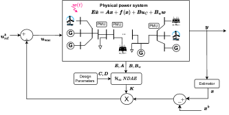
Figure 1: Overall integrated framework of the proposed control-OPF

All the simulation studies are carried out in MATLAB $2022b$ and using MATPOWER software. Optimal power flow for all the case studies is carried out by running runopf command in MATPOWER [45]. The control-OPF gain is computed via YALMIP [46] and using MOSEK [47] solver, while the power system NDAEs (5) are simulated using MATLAB DAEs solver ODE15i.

Notice that as mentioned before, the proposed control-OPF require realtime information of all the state variables as a feedback. To do that, we have used estimation algorithm given in [48]. The proposed observer in [48] require few PMUs placed optimally in the power network such that the whole system is observable and can provide accurate estimation results for both differential and algebraic states variables simultaneously. With that in mind, to compute state information we place PMUs optimally as given in [49, 50] at the following buses for different IEEE test systems; for 9-bus system at Buses $[4,6,8]$, for 14-bus system $[2,6,7,9]$, and for 39-bus and 57-bus system we place them at Buses $[3,8,10,16,20,23,25,29]$ and $[2,6,10,12,19,22,25,27,32,36,41,45,46,49,52,55,57]$ respectively. PMUs at these locations guarantees the full observability for all the test systems [49, 50]. Then, we initialize the observer from the power system equilibrium and used the technique given in [48] to perform the state estimation. Also, to further evaluate the robustness of the proposed control-OPF for all the case studies we add Gaussian noise in the PMU measurements while these computing state variables. The overall architecture of the control-OPF can be seen in Fig. 1.

TABLE I: Summary of ACOPF constraints for different test system with control-OPF for Scenario A. The results indicate no constraint violations for flows, maximum active/reactive powers.

Test System	$\max_{t}$(${\bm{S}_{f}(t)}-\bm{S}_{\mathrm{max}}$) (pu)	$\max_{t}$(${\bm{S}_{t}(t)}-\bm{S}_{\mathrm{max}})$ (pu)	$\max_{t}$(${\bm{P}_{g}(t)}-{\bm{P}_{\mathrm{max}}}$) (pu)	$\max_{t}$(${\bm{Q}_{g}(t)}-{\bm{Q}_{\mathrm{min}}}$) (pu)	$\max_{t}$(${\bm{Q}_{g}(t)}-{\bm{Q}_{\mathrm{max}}}$) (pu)
Case 9	-0.5120	-0.4401	-0.9631	3.1402	-0.1091
Case 14	-0.4101	-0.2170	-0.6706	0.1926	-0.1006
Case 39	-0.1763	-0.1695	-0.0918	2.1021	-0.1921
Case 57	-0.1391	-0.4112	-0.0111	2.1120	-1.0326

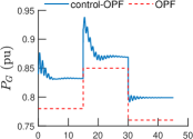
(a)

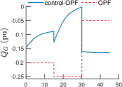
(b)

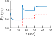
(c)

(d)

Figure 2: Time-varying active/reactive power set-points provided by control-OPF and static set-points from ACOPF for three random step disturbances in load demand; above figures are for case 39 and below figures are for case 9 test system.

(a)

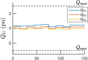
(b)

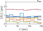
(c)

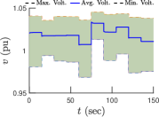
(d)

Figure 3: Active and reactive power generated by the all the generators and their respective limits, line flows and their maximum rating, and the overall modulus of all bus voltages for case 9 bus test system for Scenario A.

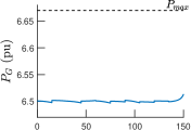
(a)

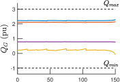
(b)

(c)

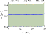
(d)

Figure 4: Active and reactive power of couple of generators and their respective limits, line flows and their maximum rating, and the overall modulus of all buses voltages for case 39 bus test system for Scenario B.

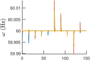
(a)

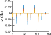
(b)

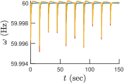
(c)

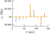
(d)

Figure 5: Generator frequencies under ten random disturbances in load and renewables for case 9, case 14, case 39, and case 57 test systems respectively.

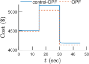
(a)

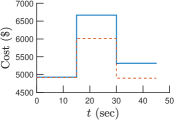
(b)

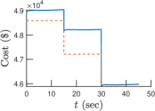
(c)

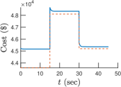
(d)

Figure 6: Comparison of the operating cost of the system with control-OPF and OPF under Scenario A, case 9, case 14, case 39, and case 57, respectively.

(a)

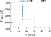
(b)

(c)

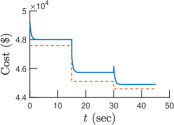
(d)

Figure 7: Comparison of the operating cost of the system with control-OPF and OPF under Scenario B, case 9, case 14, case 39, and case 57, respectively.

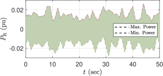
(a)

Figure 8: Random uncertainty in renewable power generations

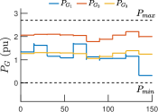
(a)

(b)

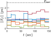
(c)

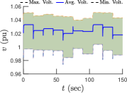
(d)

Figure 9: Active and reactive power generated by the all the generators and their respective limits, line flows and their maximum rating, and the overall modulus of all bus voltages for case 9 bus test system for Scenario B.

TABLE II: Cost comparison for the control-OPF and ACOPF for Scenario A.

System	Method	Total system cost $\times$$10^{3}$ $	Regulation cost and percentage difference from ACOPF
Case 9	ACOPF	5.4188	—
	control-OPF	5.5801	3.001
Case 14	ACOPF	8.4591	—
	control-OPF	9.0121	14.011
Case 39	ACOPF	41.819	—
	control-OPF	46.105	10.213
Case 57	ACOPF	42.771	—
	control-OPF	47.511	10.094

TABLE III: Cost comparison for the control-OPF and ACOPF for Scenario B.

System	Method	Total system cost $\times$$10^{3}$ $	Regulation cost and percentage difference from ACOPF
Case 9	ACOPF	6.3191	—
	control-OPF	6.4101	2.405
Case 14	ACOPF	10.431	—
	control-OPF	12.522	15.26
Case 39	ACOPF	52.929	—
	control-OPF	60.001	12.04
Case 57	ACOPF	50.321	—
	control-OPF	54.011	7.901

V-A Scenario A: Uncertainty in Load Demand

In this section, we analyze the overall system cost with the control-OPF and compare it with the cost obtained by running ACOPF under random disturbances in load demand. To that end, the simulations are carried out as follows: Initially, the system operates under steady-state conditions, meaning the overall demand is exactly equal to the power generated by load and renewables. Thus there are no transients in the system and the system rests in an equilibrium state. Then right after $t>0$ ten random (with varying uncertainty) step disturbances in load demand has been added as follows: $P^{\prime}_{d}+Q^{\prime}_{d}=(1+\delta_{d})(P^{0}_{d}+Q^{0}_{d})+w_{d}(t)$, where $\delta_{d}$ represent the amount of the disturbance, $w_{d}(t)$ is a Gaussian noise with zero mean and variance of $0.01(P^{0}_{d}+Q^{0}_{d})$, $P^{0}_{d}$, $Q^{0}_{d}$ are the initial active and reactive load demand, and $P^{\prime}_{d}$, $Q^{\prime}_{d}$ is the new load demand after the disturbances has been applied. For every ten simulations the value for $\delta_{d}$ is selected randomly in $[0.01,0.08]$ for case 9 and case 14, for case 39 the range is chosen in $[0.001,0.02]$, while for case 57 $\delta_{d}$ is randomly picked in $[0.001,0.01]$.

After the disturbance, the power system is stabilized via control-OPF and the gain $\bm{K}$ which is computed offline. Notice that for every load disturbance, we get time-varying generator power output vector $\bm{P}_{G}$ and $\bm{Q}_{G}$. The vector $\bm{P}_{G}$ is then plugged into the quadratic cost equation of the generators (given in MATPOWER) and finally average is taken to compute the final cost. In this way, we get the overall cost of the system with the control-OPF acting in realtime to redistribute the power from the generator in response to the disturbances. For similar uncertainties in load demand, OPF is also carried out ten times and an average of the overall cost is computed to determine the system cost for random loads with OPF.

Notice that OPF provides static set points for the vectors $\bm{P}_{G}$ and $\bm{Q}_{G}$ corresponding to each load demands. Thus the set points provided by OPF for a certain loads may not be feasible and might make the whole system unstable. On the other hand control-OPF ensures guaranteed stability and provide us time-varying set points for $\bm{P}_{G}$ and $\bm{Q}_{G}$ which make sure that system remain transiently stable and synchronized after large disturbances in loads demand.

To that end, a comparison of the overall system cost with control-OPF and OPF for this case study is presented in Tab. II. We can note that for different test networks, the average cost of system operation under various load disturbances is close to the average cost computed via just running OPF. This can also be corroborated from Fig. 6 from which we can see that the cost of control-OPF is close to the cost obtained from OPF for case 9 and case 14 test systems. Fig. 2 also illustrate the time-varying power generation set-points (for the first three simulations) generated by control-OPF and static set-points received via solving OPF and we can observe that both of them are not far away from each other. Moreover, in Fig. 3 we present active and reactive power from all the generators, line flows, and modulus of bus voltages for the case 9 test system. Notice that, line flows are computed from the state vectors as follows:

$$\bm{S}_{f}=[\bm{C}_{f}\bm{V}]\bm{Y}^{*}_{f}\bm{V}^{*},\,\,\,\,\,\bm{S}_{t}=[\bm{C}_{t}\bm{V}]\bm{Y}^{*}_{t}\bm{V}^{*}$$

where $\bm{S}_{f}$, $\bm{S}_{t}$ are apparent power flows from both ends (from bus and to bus) of the transmission line respectively, $\bm{V}$ are the bus voltages, $\bm{Y}^{*}_{f}$, $\bm{Y}^{*}_{t}$ represent the conjugate of from and to bus admittance matrices, while $\bm{C}_{f}$, $\bm{C}_{t}$ are binary matrices and it generates all from and to end buses of the transmission lines.

With that in mind, we can clearly see from Fig. 3 that all the line flows, bus voltages and generator’s power outputs are within their prescribed limits and thus the control-OPF successfully satisfies all the system constraints that are usually modeled in OPF. Similarly for all the other test systems, we can see from Tab. I that the maximum instantaneous value for the line flows, and active and reactive power generations are less than their respective maximum limits. Thus the proposed control-OPF satisfies the constraints of the system—and no ACOPF constraint violations are incurred.

TABLE IV: Summary of ACOPF constraints for different test system with the control-OPF for Scenario B. The results indicate no constraint violations for flows, maximum active/reactive powers.

Test System	$\max_{t}$(${\bm{S}_{f}(t)}-\bm{S}_{\mathrm{max}}$) (pu)	$\max_{t}$(${\bm{S}_{t}(t)}-\bm{S}_{\mathrm{max}})$ (pu)	$\max_{t}$(${\bm{P}_{g}(t)}-{\bm{P}_{\mathrm{max}}}$) (pu)	$\max_{t}$(${\bm{Q}_{g}(t)}-{\bm{Q}_{\mathrm{min}}}$) (pu)	$\max_{t}$(${\bm{Q}_{g}(t)}-{\bm{Q}_{\mathrm{max}}}$) (pu)
Case 9	-0.3009	-0.4110	-0.0401	1.2130	-1.990
Case 14	-0.1099	-0.2101	-0.1099	1.2216	-0.0115
Case 39	-0.1421	-0.7321	-0.0091	0.2510	-0.0109
Case 57	-0.7020	-0.1981	-0.0021	2.01910	-0.0307

V-B Scenario B: Uncertainty in Renewable Power Generation

Here we analyze the cost of operating the system with control-OPF and compare it with OPF under random uncertainty in renewable power generations. To that end, the simulations in this section are performed as follows: Initially, the power generation from renewables is $\bm{P}^{0}_{R}$, $\bm{Q}^{0}_{R}$, then right after $t>0$, a random disturbance has been added and the power output from renewables are given as: $P^{\prime}_{R}+Q^{\prime}_{R}=(1+\delta_{R})(P^{0}_{R}+Q^{0}_{R})+w_{R}(t)$, where $\delta_{R}$ represent the severity of the disturbance, $\bm{w}_{R}(t)$ is the random noise as shown in Fig. 8, and $P^{\prime}_{R}$, $Q^{\prime}_{R}$ are the updated power output from renewables after the disturbance. With that in mind, we carry out ten simulations and for each simulation, the value for $\delta_{R}$ is selected randomly in $[-0.01,0.03]$ for case 9 and case 14, for case 39 it is in $[-0.001,0.01]$, while for case 57 it is chosen randomly in $[-0.01,0.02]$.

To that end, from Tab. III we can see that the difference between system operating cost with control-OPF and by just running OPF are close to each other. This means that control-OPF not only ensures transient stability of the system via realtime feedback—which can be verified from Fig. 5, we can see that all the generator frequencies goes back to its equilibrium after large disturbance in load demand, but also makes sure that the power redistribution from the generators after a large disturbance is such that it is close to OPF cost. In Fig. 4 we also illustrate for the 39-bus test system the active power output of generator 2, reactive power output of generators 1 to 4, line flows of a couple of transmission lines, and modulus of bus voltages for all ten simulations. We can clearly see that for every random renewable uncertainty, the generator power output, line flows, and bus voltages are within their prescribed limits. Thus ensuring that the system constraints are satisfied.

These results can also be corroborated from Tab. IV, from which we can observe that for all test systems, the instantaneous active/reactive power outputs and transmission to and from line flows are less/greater than their respective maximum/minimum limits. Notice that the reason it satisfies all the system constraints is because the proposed control-OPF make sure that the system is transiently stable (in term of Lyapunov stability) and it inherently encodes the algebraic constraints (power balance and generator stator constraints) of power system in its feedback control architecture. To that end, since the proposed control-OPF satisfies all the system constraints and the overall system cost after a large disturbance in load and renewable is close to the cost obtained from OPF. Then the need to solve OPF after 5-10 minutes in the tertiary layer (or economic dispatch layer) of the power system can be eliminated. This is because the control-OPF acts in realtime through feedback provided by the PMUs and it also ensures system stability as discussed in Sec. IV.

We note that other types of dispatch problems are still needed, even if the control approach presented herein was able to yield cost-optimal schedules.

VI Paper Summary, Limitations, and Future Work

In this work, we propose a new method to solve the optimal power flow problem using feedback control theory. The proposed algorithm namely control-OPF is based on Lyapunov stability and it explicitly models the algebraic constraints of the power system in the controller architecture. These algebraic constraints (especially the power balance equations) are part of the OPF problem, since the control-OPF inherently satisfies these constraints then the need for solving OPF after 5-10 minutes in the tertiary layer of the power system can be rethought or potentially eliminated.

Given the case studies, we present preliminary answers to the posed research questions Q1–Q3 posed in Section V.

• A1. Depends on how you define closeness. We observe that control-OPF approach yields a cost function that is on average higher than the OPF. Results varied between 2–15% depending on the studied system and the assumed conditions.

• A2. The control-OPF approach results in no constraint violations for all studied power systems under different realizations of renewables, loads, and initial conditions.

• A3. The control-OPF produces more than just a time-varying, realtime generator setpoints and deviations; it produces realtime regulation of the grid’s voltages and frequencies. As such, one could consider the 2–15% increase in the operational system cost as a cost of realtime regulation. Who pays for this additional cost is a different story.

• A4. While the OPF knows exact values for all uncertain loads and renewables (needed to compute OPF setpoints), the control-OPF is truly uncertainty-unaware. The former needs vectors of uncertainty from renewables and loads; the latter hedges against it. Hence one could argue that the cost comparison is objectively unfair to the control-OPF. A fairer comparison would be with a stochastic OPF, that is also uncertainty unaware.

Future work will focus on comparing this framework with a robust version of ACOPF, extending the dynamic model to incorporate dynamics of renewable energy resources such as wind and solar farms, and investigating the performance of robust $\mathcal{H}_{2}$- or $\mathcal{L}_{\infty}$-based controllers in terms of costs and response to uncertainty.

References

- [1] H. W. Dommel and W. F. Tinney, “Optimal power flow solutions,” IEEE Transactions on power apparatus and systems, no. 10, pp. 1866–1876, 1968.
- [2] I. Aravena, D. K. Molzahn, S. Zhang, C. G. Petra, F. E. Curtis, S. Tu, A. Wächter, E. Wei, E. Wong, A. Gholami et al., “Recent developments in security-constrained ac optimal power flow: Overview of challenge 1 in the arpa-e grid optimization competition,” arXiv preprint arXiv:2206.07843, 2022.
- [3] J. Holzer, C. Coffrin, C. DeMarco, R. Duthu, S. Elbert, S. Greene, O. Kuchar, B. Lesieutre, H. Li, W. K. Mak et al., “Grid optimization competition challenge 2 problem formulation,” Tech. rep. ARPA-E, Tech. Rep., 2021.
- [4] J. A. Taylor, Convex optimization of power systems. Cambridge University Press, 2015.
- [5] J. Momoh, M. El-Hawary, and R. Adapa, “A review of selected optimal power flow literature to 1993. ii. newton, linear programming and interior point methods,” IEEE Transactions on Power Systems, vol. 14, no. 1, pp. 105–111, 1999.
- [6] R. P. O. M. B. Cain and A. Castillo, “History of optimal power flow and formulations,” pp. 1–36, Nov 2021. [Online]. Available: https://www.ferc.gov/sites/default/files/2020-05/acopf-1-history-formulation-testing.pdf
- [7] A. J. Ardakani and F. Bouffard, “Identification of umbrella constraints in dc-based security-constrained optimal power flow,” IEEE Transactions on Power Systems, vol. 28, no. 4, pp. 3924–3934, 2013.
- [8] M. S. Andersen, A. Hansson, and L. Vandenberghe, “Reduced-complexity semidefinite relaxations of optimal power flow problems,” IEEE Transactions on Power Systems, vol. 29, no. 4, pp. 1855–1863, 2014.
- [9] R. Louca, P. Seiler, and E. Bitar, “A rank minimization algorithm to enhance semidefinite relaxations of optimal power flow,” in 2013 51st Annual Allerton Conference on Communication, Control, and Computing (Allerton), 2013, pp. 1010–1020.
- [10] J. Lavaei and S. H. Low, “Zero duality gap in optimal power flow problem,” IEEE Transactions on Power Systems, vol. 27, no. 1, pp. 92–107, 2012.
- [11] D. K. Molzahn, B. C. Lesieutre, and C. L. DeMarco, “A sufficient condition for global optimality of solutions to the optimal power flow problem,” IEEE Transactions on Power Systems, vol. 29, no. 2, pp. 978–979, 2014.
- [12] D. K. Molzahn, J. T. Holzer, B. C. Lesieutre, and C. L. DeMarco, “Implementation of a large-scale optimal power flow solver based on semidefinite programming,” IEEE Transactions on Power Systems, vol. 28, no. 4, pp. 3987–3998, 2013.
- [13] S. H. Low, “Convex relaxation of optimal power flow—part i: Formulations and equivalence,” IEEE Transactions on Control of Network Systems, vol. 1, no. 1, pp. 15–27, 2014.
- [14] R. Madani, S. Sojoudi, and J. Lavaei, “Convex relaxation for optimal power flow problem: Mesh networks,” IEEE Transactions on Power Systems, vol. 30, no. 1, pp. 199–211, 2015.
- [15] R. Madani, M. Ashraphijuo, and J. Lavaei, “Promises of conic relaxation for contingency-constrained optimal power flow problem,” IEEE Transactions on Power Systems, vol. 31, no. 2, pp. 1297–1307, 2016.
- [16] A. Gopalakrishnan, A. U. Raghunathan, D. Nikovski, and L. T. Biegler, “Global optimization of optimal power flow using a branch & bound algorithm,” in 2012 50th Annual Allerton Conference on Communication, Control, and Computing (Allerton). IEEE, 2012, pp. 609–616.
- [17] M. Lu, H. Nagarajan, R. Bent, S. D. Eksioglu, and S. J. Mason, “Tight piecewise convex relaxations for global optimization of optimal power flow,” in 2018 Power Systems Computation Conference (PSCC). IEEE, 2018, pp. 1–7.
- [18] D. Lee, K. Turitsyn, D. K. Molzahn, and L. A. Roald, “Feasible path identification in optimal power flow with sequential convex restriction,” IEEE Transactions on Power Systems, vol. 35, no. 5, pp. 3648–3659, 2020.
- [19] K. Baker, “Learning warm-start points for ac optimal power flow,” in 2019 IEEE 29th International Workshop on Machine Learning for Signal Processing (MLSP). IEEE, 2019, pp. 1–6.
- [20] W. Huang, X. Pan, M. Chen, and S. H. Low, “Deepopf-v: Solving ac-opf problems efficiently,” IEEE Transactions on Power Systems, vol. 37, no. 1, pp. 800–803, 2022.
- [21] X. Pan, T. Zhao, M. Chen, and S. Zhang, “Deepopf: A deep neural network approach for security-constrained dc optimal power flow,” IEEE Transactions on Power Systems, vol. 36, no. 3, pp. 1725–1735, 2021.
- [22] A. S. Zamzam and K. Baker, “Learning optimal solutions for extremely fast ac optimal power flow,” in 2020 IEEE International Conference on Communications, Control, and Computing Technologies for Smart Grids (SmartGridComm), 2020, pp. 1–6.
- [23] K. Baker, “Emulating ac opf solvers with neural networks,” IEEE Transactions on Power Systems, vol. 37, no. 6, pp. 4950–4953, 2022.
- [24] Y. Zhou, B. Zhang, C. Xu, T. Lan, R. Diao, D. Shi, Z. Wang, and W.-J. Lee, “A data-driven method for fast ac optimal power flow solutions via deep reinforcement learning,” Journal of Modern Power Systems and Clean Energy, vol. 8, no. 6, pp. 1128–1139, 2020.
- [25] M. Bazrafshan, N. Gatsis, A. F. Taha, and J. A. Taylor, “Coupling load-following control with opf,” IEEE Transactions on Smart Grid, vol. 10, no. 3, pp. 2495–2506, 2019.
- [26] N. Li, C. Zhao, and L. Chen, “Connecting automatic generation control and economic dispatch from an optimization view,” IEEE Transactions on Control of Network Systems, vol. 3, no. 3, pp. 254–264, 2016.
- [27] F. Dorfler, J. W. Simpson-Porco, and F. Bullo, “Breaking the hierarchy: Distributed control and economic optimality in microgrids,” IEEE Transactions on Control of Network Systems, vol. 3, no. 3, pp. 241–253, 2016.
- [28] S. Trip, M. Bürger, and C. De Persis, “An internal model approach to (optimal) frequency regulation in power grids with time-varying voltages,” Automatica, vol. 64, pp. 240–253, 2016. [Online]. Available: https://www.sciencedirect.com/science/article/pii/S0005109815004859
- [29] Y. Tang, K. Dvijotham, and S. Low, “Real-time optimal power flow,” IEEE Transactions on Smart Grid, vol. 8, no. 6, pp. 2963–2973, 2017.
- [30] P. Sauer, M. Pai, and J. Chow, Power System Dynamics and Stability: With Synchrophasor Measurement and Power System Toolbox, ser. Wiley - IEEE. Wiley, 2017.
- [31] K. Zhou and J. C. Doyle, Essentials of robust control. Prentice Hall, 1998, vol. 104.
- [32] S. Boyd, L. El Ghaoui, E. Feron, and V. Balakrishnan, Linear matrix inequalities in system and control theory. SIAM, 1994.
- [33] P. M. C. Derinkuyu, Kurşad, “On the s-procedure and some variants,” Mathematical Methods of Operations Research, vol. 64, no. 1, pp. 55–77, 2016.
- [34] F. Zhang, The Schur complement and its applications. Springer Science & Business Media, 2006, vol. 4.
- [35] A. K. Singh and B. C. Pal, “Decentralized control of oscillatory dynamics in power systems using an extended lqr,” IEEE Transactions on Power Systems, vol. 31, no. 3, pp. 1715–1728, 2016.
- [36] T. Sadamoto, A. Chakrabortty, T. Ishizaki, and J.-i. Imura, “Dynamic modeling, stability, and control of power systems with distributed energy resources: Handling faults using two control methods in tandem,” IEEE Control Systems Magazine, vol. 39, no. 2, pp. 34–65, 2019.
- [37] M. Nadeem, M. Bahavarnia, and A. F. Taha, “On wide-area control of solar-integrated dae models of power grids,” in 2023 American Control Conference (ACC). IEEE, 2023, pp. 4495–4500.
- [38] S. A. Nugroho and A. F. Taha, “Load-and renewable-following control of linearization-free differential algebraic equation power system models,” IEEE Transactions on Control Systems Technology, 2023.
- [39] N. Li, C. Zhao, and L. Chen, “Connecting automatic generation control and economic dispatch from an optimization view,” IEEE Transactions on Control of Network Systems, vol. 3, no. 3, pp. 254–264, 2015.
- [40] Z. Miao and L. Fan, “Achieving economic operation and secondary frequency regulation simultaneously through local feedback control,” IEEE Transactions on Power Systems, vol. 32, no. 1, pp. 85–93, 2016.
- [41] D. B. Eidson and M. D. Ilic, “Advanced generation control with economic dispatch,” in Proceedings of 1995 34th IEEE Conference on Decision and Control, vol. 4. IEEE, 1995, pp. 3450–3458.
- [42] C. Zhao, E. Mallada, S. H. Low, and J. Bialek, “Distributed plug-and-play optimal generator and load control for power system frequency regulation,” International Journal of Electrical Power & Energy Systems, vol. 101, pp. 1–12, 2018.
- [43] E. Mallada, C. Zhao, and S. Low, “Optimal load-side control for frequency regulation in smart grids,” IEEE Transactions on Automatic Control, vol. 62, no. 12, pp. 6294–6309, 2017.
- [44] C. Zhao, E. Mallada, and S. H. Low, “Distributed generator and load-side secondary frequency control in power networks,” in 2015 49th Annual Conference on Information Sciences and Systems (CISS). IEEE, 2015, pp. 1–6.
- [45] R. D. Zimmerman, C. E. Murillo-Sánchez, and R. J. Thomas, “Matpower: Steady-state operations, planning, and analysis tools for power systems research and education,” IEEE Transactions on Power Systems, vol. 26, no. 1, pp. 12–19, 2011.
- [46] J. Löfberg, “Yalmip : A toolbox for modeling and optimization in matlab,” in In Proceedings of the CACSD Conference, Taipei, Taiwan, 2004.
- [47] E. D. Andersen and K. D. Andersen, The Mosek Interior Point Optimizer for Linear Programming: An Implementation of the Homogeneous Algorithm. Boston, MA: Springer US, 2000, pp. 197–232.
- [48] M. Nadeem, S. A. Nugroho, and A. F. Taha, “Dynamic state estimation of nonlinear differential algebraic equation models of power networks,” IEEE Transactions on Power Systems, vol. 38, no. 3, pp. 2539–2552, 2022.
- [49] N. M. Manousakis and G. N. Korres, “A weighted least squares algorithm for optimal pmu placement,” IEEE Transactions on Power Systems, vol. 28, no. 3, pp. 3499–3500, 2013.
- [50] S. Chakrabarti and E. Kyriakides, “Optimal placement of phasor measurement units for power system observability,” IEEE Transactions on Power Systems, vol. 23, no. 3, pp. 1433–1440, 2008.