Don’t Bet on Luck Alone: Enhancing Behavioral Reproducibility of Quality-Diversity Solutions in Uncertain Domains

Abstract.

Quality-Diversity (QD) algorithms are designed to generate collections of high-performing solutions while maximizing their diversity in a given descriptor space. However, in the presence of unpredictable noise, the fitness and descriptor of the same solution can differ significantly from one evaluation to another, leading to uncertainty in the estimation of such values. Given the elitist nature of QD algorithms, they commonly end up with many degenerate solutions in such noisy settings. In this work, we introduce Archive Reproducibility Improvement Algorithm (ARIA); a plug-and-play approach that improves the reproducibility of the solutions present in an archive. We propose it as a separate optimization module, relying on natural evolution strategies, that can be executed on top of any QD algorithm. Our module mutates solutions to (1) optimize their probability of belonging to their niche, and (2) maximize their fitness. The performance of our method is evaluated on various tasks, including a classical optimization problem and two high-dimensional control tasks in simulated robotic environments. We show that our algorithm enhances the quality and descriptor space coverage of any given archive by at least 50%.

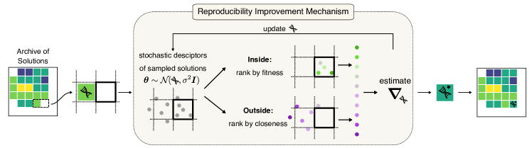
Figure 1. One iteration of the Archive Reproducibility Improvement Algorithm (ARIA) during the ”completion phase”. Two adjacent cells are selected such that one, the target cell, is empty while the other one is already populated by a solution. Then, the Reproducibility Improvement Mechanism uses this solution as a starting point for finding a high-performing solution in the target cell. After several steps of Reproducibility Improvement, we add the resulting optimized solution to the target cell.

1. Introduction

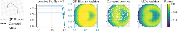
Figure 2. Archive Profile, Illusory archive, and the corresponding corrected archive returned by ARIA- ME init on the Arm task. The ARIA archive shows the result obtained after optimization from ARIA.

Quality-Diversity (QD) Algorithms (Pugh et al., 2015, 2016; Cully and Demiris, 2018b) are evolutionary algorithms designed to produce collections, or archives, of diverse and high-performing solutions. These archives can then be used for various applications, including damage recovery in robotics (Cully et al., 2015; Allard et al., 2022; Kaushik et al., 2020; Chatzilygeroudis et al., 2018), video-game design (Fontaine et al., 2020a; Earle et al., 2022), and configuring urban layouts (Galanos et al., 2021).

QD approaches rely on an evaluation process which is used to estimate the performance of a given solution; for each solution an evaluation also results in a descriptor which characterizes the novelty of that solution compared to the others. Most QD algorithms are designed under the assumption that this evaluation process is deterministic. Deterministic here means that the evaluation of a solution always returns the same result (fitness and descriptor). However, realistically, there are many contexts and applications in which uncertainty is present in the evaluation process. For example, in robotics, the measurements from a sensor may be noisy and applying a command to an actuator may not lead to the exact desired displacement; in those cases, sending a command to a robot may not always return the same results. QD setups where the domain presents uncertainty belong to the Uncertain QD framework (Flageat and Cully, 2023). If QD algorithms are not designed to take this uncertainty into account, they may produce ”illusory” archives, with many solutions whose performance and descriptors are wrongly estimated and may exhibit a high variance (Flageat and Cully, 2023). In such cases, we say that the solutions have low reproducibility. To have highly reproducible solutions, they need to have a low variance and good descriptor and performance estimations.

In this work, we introduce the Archive Reproducibility Improvement Algorithm (ARIA) a method that lowers down the solution’s variance, i.e. increases their reproducibility. It can be used as a plug-and-play tool, applicable to any set of solutions, including solutions returned by QD and Evolution Strategy algorithms. It relies on a Reproducibility Improvement Mechanism (Fig. 1) which uses natural evolution strategies to decrease the descriptor variance of a solution and also maximize its fitness. We leverage this mechanism to not only increase the reproducibility of solutions present in an archive, but also to discover new solutions, hence increasing the diversity of a given archive (Fig. 2). We compare ARIA with different reproducibility-aware baselines on three classical Uncertain QD tasks, and show that ARIA finds the best archives, both in terms of performance and reproducibility. More specifically, compared to standard baselines, the best variants of ARIA achieve a 30% higher QD-Score, and improve the reproducibility by at least 20%.

2. Background

2.1. Evolution Strategies

In this work, we intend to use ES optimization algorithms that are applicable to possibly high-dimensional problems, including deep neuroevolution tasks. Salimans et al. (2017) proposes a method that takes inspiration from Natural Evolution Strategies (Wierstra et al., 2014): instead of optimizing directly for an objective function $\widetilde{o}(\cdot)$, they maximize the expectation of $\widetilde{o}$ under a Gaussian distribution: $\mbox{E}_{{{\bm{{\theta}}}\sim\mathcal{N}({\bm{{\phi}}},\sigma^{2}{\bm{{I}}})}}\left[{\widetilde{o}({\bm{{\theta}}})}\right]$ where the mean ${\bm{{\phi}}}$ is the variable to optimize, and the standard deviation $\sigma$ is kept constant. It is common in ES to use rank-based utility values $(u_{s})$ instead of the objective values (Wierstra et al., 2014; Hansen, 2016). In that case, the gradient used to update the parameters can be expressed: $\frac{1}{\sigma}\sum_{s=1}^{N_{\mbox{s}}}u_{s}{\bm{{\epsilon}}}_{s}$, where ${\bm{{\epsilon}}}_{s}$ is sampled from a normal distribution.

2.2. Quality-Diversity Algorithms

Quality-Diversity (QD) algorithms (Pugh et al., 2015; Cully and Demiris, 2018b) aim at finding a collection, also called ”archive”, of diverse and high-performing solutions to an optimization problem. Unlike common evolutionary algorithms, QD algorithms consider that solutions are not only assigned a fitness, but also a descriptor used to measure their novelty. Common QD algorithms such as MAP-Elites (Mouret and Clune, 2015; Cully et al., 2015) discretize this descriptor space into a grid. For each cell of this grid, those algorithms intend to find one solution whose descriptor is in the cell, and whose fitness maximizes the performance in that cell. At each iteration, they operate as follow: solutions are selected from the archive and modified via random variations (e.g. mutations, cross-overs…); then their fitness and descriptors are evaluated, and they are added back to the archive. More precisely, to add a solution to the archive, we first check which cell its descriptor belongs to. If this cell is empty, then the solution is added to the cell; otherwise, if the cell is already occupied by another solution, only the best-performing solution is kept. With those mechanisms, MAP-Elites and its variants progressively increase the number of cells filled, while also improving the performance of the solutions stored in the archive.

2.3. Uncertain QD Setting with Descriptor Reproducibility Maximization

There are environments for which successive evaluations of the same solution may lead to different results. For example in robotics, this is often due to different initial conditions, noise from the sensors, or looseness in the joints. In the Uncertain QD Setting, formalized by Flageat and Cully (2023), successive evaluations of the same solution ${\bm{{\theta}}}$ may lead to different fitnesses and descriptors. In such setting, the fitness $f$ and descriptor ${\bm{{d}}}$ resulting from a solution ${\bm{{\theta}}}$ can be represented as two distributions $\mathcal{D}_{f}^{({\bm{{\theta}}})}$ and $\mathcal{D}_{d}^{({\bm{{\theta}}})}$. Considering a descriptor space partitioned into cells $\left(\mathcal{C}_{i}\right)$, the problem can be expressed as: for each cell $\mathcal{C}_{i}$, we intend to find a solution ${\bm{{\theta}}}_{i}$ maximizing the expected fitness $\mbox{E}_{{f_{i}\sim\mathcal{D}_{d}^{({\bm{{\theta}}}_{i})}}}\left[{f_{i}}\right]$ while the expected descriptor $\mbox{E}_{{{\bm{{d}}}_{i}\sim\mathcal{D}_{d}^{({\bm{{\theta}}}_{i})}}}\left[{{\bm{{d}}}_{i}}\right]$ belongs to the the cell $\mathcal{C}_{i}$. Additionally, we aim at minimizing the variance of the descriptor components over each descriptor dimension $j$. In other words, we consider the following multi-objective constrained optimization problems:

(P1) $$\begin{split}\text{For each cell $\mathcal{C}_{i}$, }&\text{find a solution ${\bm{{\theta}}}_{i}$ that:}\\ &\mbox{maximize}\>\mbox{E}_{{f_{i}\sim\mathcal{D}_{f}^{({\bm{{\theta}}}_{i})}}}\left[{f_{i}}\right]\\ &\mbox{minimize}\>\mbox{Var}_{{{\bm{{d}}}_{i}\sim\mathcal{D}_{d}^{({\bm{{\theta}}}_{i})}}}\left[{{\bm{{d}}}_{i}^{(j)}}\right]\;\forall j\\ &\mbox{subject to}\>\mbox{E}_{{{\bm{{d}}}_{i}\sim\mathcal{D}_{d}^{({\bm{{\theta}}}_{i})}}}\left[{{\bm{{d}}}_{i}}\right]\in\mathcal{C}_{i}\end{split}$$

Algorithm 1 ARIA

1:Input: set of genotypes given by an ES or QD algorithm $\Phi$; number gradient steps $N_{\mbox{grad}}$; Number samples per gradient step $N_{\mbox{s}}$; standard deviation samples $\sigma$

2:$\mathcal{P}_{\mbox{expl}}\leftarrow\emptyset$, $\mathcal{P}_{\mbox{targ}}\leftarrow$ all cells partitioning the descriptor space

3:$\triangleright$ Reproducibility Improvement Phase

4:for  genotype ${\bm{{\phi}}}\in\Phi$ do

5:    $({\bm{{d}}}_{s})_{s=1}^{N_{\mbox{s}}}\leftarrow$ evaluate genotype $N_{\mbox{s}}$ times and collect descriptors

6:    $\mathcal{C}_{j}\leftarrow$ find cell containing mean descriptor $\overline{{\bm{{d}}}}$

7:    ${\bm{{\phi}}}_{j}\leftarrow$ Reproducibility Improvement (${\bm{{\phi}}}_{\mbox{init}}={\bm{{\phi}}}$, $\mathcal{C}_{\mbox{targ}}=\mathcal{C}_{j}$, $N_{\mbox{grad}}$, $N_{\mbox{s}}$, $\sigma$)

8:    Add $\mathcal{C}_{j}$ to $\mathcal{P}_{\mbox{expl}}$, and remove it from $\mathcal{P}_{\mbox{targ}}$

9:$\triangleright$ Archive Completion Phase

10:while $\mathcal{P}_{\mbox{targ}}$ is not empty do

11:    Select 2 adjacent cells such that $\mathcal{C}_{\mbox{s}}\in\mathcal{P}_{\mbox{expl}}$ and $\mathcal{C}_{\mbox{targ}}\in\mathcal{P}_{\mbox{targ}}$

12:    ${\bm{{\phi}}}_{\mbox{s}}\leftarrow$ genotype associated to $\mathcal{C}_{\mbox{s}}$

13:    ${\bm{{\phi}}}_{\mbox{targ}}\leftarrow$ Reproducibility Improvement (${\bm{{\phi}}}_{\mbox{init}}={\bm{{\phi}}}_{\mbox{s}}$, $\mathcal{C}_{\mbox{targ}}$, $N_{\mbox{grad}}$, $N_{\mbox{s}}$, $\sigma$ )

14:    Add ${\bm{{\phi}}}_{\mbox{targ}}$ to the target cell $\mathcal{C}_{\mbox{targ}}$

15:    Add $\mathcal{C}_{\mbox{targ}}$ to $\mathcal{P}_{\mbox{expl}}$, and remove it from $\mathcal{P}_{\mbox{targ}}$

16:

17:return all genotypes from all cells

2.4. Related Work

QD in Uncertain Domains

The issue of QD applied to uncertain domains has incrementally emerged in recent literature following advances in QD toward neuroevolution and complex robotics applications (Flageat et al., 2022b). When faced with uncertainty, QD algorithms struggle to estimate the expected quality and novelty of solutions. Multiple variants of MAP-Elites have been proposed to address this limitation. Such variants either rely on sampling solutions multiple times - dynamically (Justesen et al., 2019; Flageat and Cully, 2023) or not (Cully and Demiris, 2018a) -, or rely on more complex mechanisms based on previous individuals (Flageat and Cully, 2020, 2023). Additionally, gradient-augmented QD approaches such as PGA-MAP-Elites (Nilsson and Cully, 2021) and MAP-Elites-ES (Colas et al., 2020) have also proven promising in tackling the issue of uncertainty. Their informed gradient-based mechanism allows them to produce more reproducible solutions than vanilla QD approaches (Flageat et al., 2022a). However, all these previous works rely on modifying the main MAP-Elites algorithm to directly produce better estimates of performance and encourage reproducible solutions. In comparison, our approach ARIA proposes a plug-and-play mechanism that improves the result of any given QD algorithm, even those which do not take into account the uncertainty of the task.

Mixing QD with ES

Multiple previous works proposed to integrate ES within MAP-Elites. Notably, the CMA-ME algorithm (Fontaine et al., 2020b) proposed to use CMA-ES to generate offspring for MAP-Elites. Similarly to ARIA, CMA-ME optimizes for objectives distinct from the raw task fitness, such as the archive improvement score. Closer to our work, MAP-Elites-ES (Colas et al., 2020) uses the Natural ES (Wierstra et al., 2014) from Salimans et al. (2017) to produce offspring within MAP-Elites, optimizing either for the task fitness or the solution novelty. These two approaches improve upon MAP-Elites by integrating an ES mechanism within the mutation procedure of QD, while ARIA proposes to apply the ES mechanism as a second step, on top of the chosen QD algorithm. Also, the objective function used by ARIA is different from those employed by CMA-ME and MAP-Elites-ES. Indeed, the objective function of ARIA is designed to primarily optimize the reproducibility of solutions. Furthermore, CMA-ME and MAP-Elites-ES could both be used as initialization algorithms for ARIA.

Previous work in targeted improvement for QD

Distinct branches of work developed mechanisms to select efficient optimization starting-points in a QD archive. MAP-Elites-ES (Colas et al., 2020) relies on a biased parent-selection mechanism; this mechanism selects parents that tend to produce offspring solutions with a higher fitness or novelty. Similarly, Go-Explore (Ecoffet et al., 2021) solves hard-exploration tasks by selecting relevant cells to explore from. During ARIA’s final phase, its selection mechanism iteratively selects a solution at the border of the discovered descriptor space, and optimizes it to find a new solution in an empty adjacent cell, as illustrated on Figure 1.

3. Methods

In this section, we first describe an alternative problem formulation to the Uncertain QD problem P1. Then, we describe the Archive Reproducibility Improvement Algorithm (ARIA), a plug-and-play approach that can optimize a set of solutions to produce an archive of diverse, high-performing and reproducible solutions. Finally, we provide more details regarding the Reproducibility Improvement Mechanism on which ARIA relies.

3.1. Problem Definition

As explained in Section 2.3, the Uncertain QD problem can be formalized as a multi-objective problem where the descriptor variances are minimized, and the expected fitness inside each cell is maximized (see Problem P1). However, this optimization problem is computationally challenging to solve directly. Instead of minimizing the variance in the descriptor space, we propose to maximize the probability that the descriptor of each solution belongs to its designated cell. Thanks to this, problem P1 becomes:

(P2) $$\begin{split}\text{For each cell $\mathcal{C}_{i}$, }&\text{find a solution ${\bm{{\theta}}}_{i}$ that:}\\ &\mbox{maximize}\>\mbox{E}_{{f_{i}\sim\mathcal{D}_{f}^{({\bm{{\theta}}}_{i})}}}\left[{f_{i}}\right]\\ &\mbox{maximize}\>\mbox{P}\left({{\bm{{d}}}_{i}\in\mathcal{C}_{\mbox{targ}}}\right)\\ &\mbox{subject to}\>\mbox{E}_{{{\bm{{d}}}_{i}\sim\mathcal{D}_{d}^{({\bm{{\theta}}}_{i})}}}\left[{{\bm{{d}}}_{i}}\right]\in\mathcal{C}_{i}\end{split}$$

The descriptor variance, as expressed in Problem P1, is correlated with the new probability objective. By maximizing $\mbox{P}\left({{\bm{{d}}}_{i}\in\mathcal{C}_{i}}\right)$, we minimize a lower bound on the trace of the covariance matrix (see proof in Appendix A).

3.2. ARIA Outline

In this work, we propose the Archive Reproducibility Improvement Algorithm (ARIA), that addresses problem P2. ARIA takes as input a set of solutions; this set of solutions can be an archive returned by a QD algorithm, or even a single optimized solution returned by an ES algorithm. Thus, ARIA is a plug-and-play approach which can be applied to any set of solutions returned by a QD or ES algorithm; it returns an archive with high-performing and diverse solutions that are also highly reproducible. The outline of ARIA can be divided into two successive phases, all detailed in Algorithm 1:

1. The Reproducibility Improvement phase: improves the reproducibility of the solutions provided as input, by using a Reproducibility Improvement Mechanism.

2. The Archive Completion phase: uses the same Reproducibility Improvement Mechanism to find high-performing and reproducible solutions in the archive cells that are still empty.

3.2.1. Reproducibility Improvement Phase

The Reproducibility Improvement phase aims at improving the reproducibility of the solutions provided as input to the algorithm. To that end, for each solution in the input set, we reevaluate it $N_{\mbox{s}}$ times and we calculate their mean descriptor; the mean descriptor is defined as the average of the descriptors observed from $N_{\mbox{s}}$ reevaluations of the same solution. Then we check which cell $\mathcal{C}_{\mbox{targ}}$ contains this mean descriptor. And we use our Reproducibility Improvement Mechanism to optimize for the performance and reproducibility of the solution with respect to the cell $\mathcal{C}_{\mbox{targ}}$. This Reproducibility Improvement Mechanism consists of using an ES to optimize this solution for $N_{\mbox{grad}}$ steps; more details are provided below. Those steps are detailed in Algorithm 1 on lines 4-8.

3.2.2. Archive Completion Phase

At the end of the Reproducibility Improvement Phase, there are still some cells in the grid that are not covered. For example, there is no input solution whose mean descriptor ends in a cell, then this cell is still empty at the end of the previous phase. Therefore, after having improved the reproducibility of all initial solutions, we have two complementary sets of cells: $\mathcal{P}_{\mbox{expl}}$ and $\mathcal{P}_{\mbox{targ}}$. The $\mathcal{P}_{\mbox{expl}}$ contains all the cells that have been used as targets by Reproducibility Improvement so far. The purpose of this phase is to find controllers populating the remaining cells to explore $\mathcal{P}_{\mbox{targ}}$. To do that, we explore the remaining cells from $\mathcal{P}_{\mbox{targ}}$ step by step, as depicted on Figure 1.

At each iteration loop, we start by selecting a pair of cells $\mathcal{C}_{\mbox{s}}$, and $\mathcal{C}_{\mbox{targ}}$ satisfying three conditions: (i) $\mathcal{C}_{\mbox{s}}\in\mathcal{P}_{\mbox{expl}}$, (ii) $\mathcal{C}_{\mbox{targ}}\in\mathcal{P}_{\mbox{targ}}$, and (iii) $\mathcal{C}_{\mbox{s}}$ and $\mathcal{C}_{\mbox{targ}}$ are adjacent. Then, we take the initial solution ${\bm{{\phi}}}_{\mbox{init}}$ from $\mathcal{C}_{\mbox{s}}$, and use Reproducibility Improvement to optimize its fitness and its probability to fall into $\mathcal{C}_{\mbox{targ}}$. In the end, we collect the solution resulting from this optimization procedure ${\bm{{\phi}}}_{\mbox{togo}}$. Note that nothing prevents the mean descriptor of the optimized solution ${\bm{{\phi}}}_{\mbox{togo}}$from not being in the target cell $\mathcal{C}_{\mbox{targ}}$. This can happen if the descriptor cell is not reachable, or if the Reproducibility Improvement Mechanism ends too early. In any case, we add ${\bm{{\phi}}}_{\mbox{togo}}$ to the target cell $\mathcal{C}_{\mbox{targ}}$; and we add $\mathcal{C}_{\mbox{targ}}$ to the set of explored cells $\mathcal{P}_{\mbox{expl}}$, and remove it from $\mathcal{P}_{\mbox{targ}}$. We repeat the previous steps until there are no more cells to explore. All those details are provided in Algorithm 1 from line 10 onward.

3.3. Reproducibility Improvement Mechanism

Algorithm 2 Reproducibility Improvement

1:Input: Initial genotype ${\bm{{\phi}}}_{\mbox{init}}$, Cell $\mathcal{C}_{\mbox{targ}}$, Number gradient steps $N_{\mbox{grad}}$, Number samples per gradient step $N_{\mbox{s}}$, Standard deviation sampling $\sigma$

2:${\bm{{\phi}}}\leftarrow{\bm{{\phi}}}_{\mbox{init}}$

3:for $\mbox{step}=1\rightarrow N_{\mbox{grad}}$ do

4:    for $s=1\rightarrow N_{\mbox{s}}$ do

5:        Sample ${\bm{{\epsilon}}}_{s}\sim\mathcal{N}({\bm{{0}}},{\bm{{I}}})$

6:        $f_{s},{\bm{{d}}}_{s}\leftarrow$ stochastic evaluation of genotype ${\bm{{\theta}}}_{s}={\bm{{\phi}}}+\sigma{\bm{{\epsilon}}}_{s}$     

7:    $\left(u_{s}\right)\leftarrow$ rank-based utility values depending on their order for objective $o_{\mathcal{C}_{\mbox{targ}}}$ (Eq. 1)

8:    $\mbox{gradient\_estimate}\leftarrow\frac{1}{\sigma}\sum_{s=1}^{N_{\mbox{s}}}u_{s}{\bm{{\epsilon}}}_{s}$

9:    ${\bm{{\phi}}}\leftarrow$ perform gradient ascent step on ${\bm{{\phi}}}$ using gradient_estimate

10:return final genotype ${\bm{{\phi}}}$

As explained in the previous section, the Reproducibility Improvement Mechanism takes as input a solution to be optimized, and a target cell $\mathcal{C}_{\mbox{targ}}$. This mechanism aims at optimizing the solution’s expected fitness and probability of belonging to $\mathcal{C}_{\mbox{targ}}$, while also satisfying the constraint: having its mean descriptor belonging to $\mathcal{C}_{\mbox{targ}}$ (see Problem P2). To address this constrained optimization problem for a particular target cell $\mathcal{C}=\mathcal{C}_{\mbox{targ}}$ and its associated centroid ${\bm{{c}}}$, we rely on the ES of Salimans et al. (2017), detailed in Section 2.1 and in Algorithm 2.

This ES algorithm iteratively updates a solution ${\bm{{\phi}}}$ by (1) sampling and evaluating neighboring solutions in the search space following a Gaussian distribution, (2) ranking those solutions by order of preference, and (3) updating ${\bm{{\phi}}}$ following the estimated rank-based gradient (see Section 2.1). In order to improve the reproducibility of ${\bm{{\phi}}}$, we rank the solutions in the following manner:

• All solutions whose evaluated descriptor is in the cell, are ranked higher than those outside of the cell.

• Among the solutions whose descriptors are outside the cell, solutions are ranked according to their distance to the center of the cell: the closer the better.

• Among the solutions whose descriptors are inside the cell, solutions are ranked according to their fitness: the higher the better.

More formally, this is equivalent to maximizing the following objective function, which satisfies all the above ranking rules:

(1) $$\widetilde{o}_{\mathcal{C}}({\bm{{\theta}}}) =o_{\mathcal{C}}(f,{\bm{{d}}})\quad\text{with $f$ and ${\bm{{d}}}$ sampled from $\mathcal{D}_{f}^{({\bm{{\theta}}})},\mathcal{D}_{d}^{({\bm{{\theta}}})}$}$$

$$=\begin{cases}f\quad&\mbox{if }{\bm{{d}}}\in\mathcal{C}\\ f_{\mbox{min}}-\left\lVert{\bm{{d}}}-{\bm{{c}}}\right\rVert_{2}\quad&\mbox{if }{\bm{{d}}}\notin\mathcal{C}\end{cases}$$

This structure of objective function has been proposed in the evolutionary literature as a way to address constrained optimization problems (Coello, 2002; Hansen, 2016). Note that the function $\widetilde{o}(\cdot)$ is stochastic, while the function $o(\cdot)$ is a deterministic function of the sampled fitness and descriptor. Additionally, if we make the assumption that the fitness is bounded, it is provable that by maximizing the expectation of $\widetilde{o}_{\mathcal{C}_{\mbox{targ}}}(\cdot)$, we maximize a lower bound on the two objectives of Problem P2, namely: the expected fitness and the probability of belonging to a descriptor cell (see proof in Appendix A).

4. Experimental Setup

4.1. Metrics

4.1.1. Expected Fitness (EF) and (Corrected) QD-Score

The Expected Fitness (EF) (Flageat et al., 2022b) characterizes the average performance of a solution with respect to the task. As given in Problems P1 and P2, it is one of the quantities explicitly maximized for in our algorithms. To estimate the expected fitness of one solution, we reevaluate it $M$ times, and average the obtained fitnesses.

(2) $$\mbox{EF}({\bm{{\theta}}})=\mbox{E}_{{f\sim\mathcal{D}_{f}^{({\bm{{\theta}}})}}}\left[{f}\right]\approx\frac{1}{M}\sum_{m=1}^{M}f_{m}\quad\mbox{with }f_{m}\sim\mathcal{D}_{f}^{({\bm{{\theta}}})}$$

The (Corrected) QD-Score (Pugh et al., 2015; Flageat et al., 2022b) characterizes both the quality and diversity of an archive. It corresponds to the sum of all the expected fitnesses of solutions contained in an archive. To cope with negative values, all expected fitnesses are first normalized between $0$ and $1$ before being summed.

4.1.2. Negated Descriptor Variance (NDV) and Variance Score (V-Score)

The NDV (Flageat and Cully, 2023) characterizes the spread of the descriptor samples. Mathematically, it corresponds to the negated trace of the covariance matrix of the descriptor samples. If a solution has a high NDV score, i.e. an NDV score close to $0$, it means that its sample descriptors are (in average) concentrated around their mean. This metric comes from the variance objective that we minimize in our original Uncertain QD problem (see Problem P1). We evaluate it with the following unbiased estimator (where $\overline{{\bm{{d}}}}=\frac{1}{M}\sum_{m=1}^{M}{\bm{{d}}}_{m}$):

$$\mbox{NDV}({\bm{{\theta}}}) =-\sum_{j}\mbox{Var}_{{{\bm{{d}}}\sim\mathcal{D}_{d}^{({\bm{{\theta}}})}}}\left[{{\bm{{d}}}^{(j)}}\right]$$

$$\approx\frac{-1}{M-1}\sum_{m=1}^{M}\left\lVert{\bm{{d}}}_{m}-\overline{{\bm{{d}}}}\right\rVert_{2}^{2}\quad\text{with }{\bm{{d}}}_{m}\sim\mathcal{D}_{d}^{({\bm{{\theta}}})}$$

The Variance Score (V-Score) is the NDV equivalent of the QD-Score. Instead of considering normalized expected fitnesses, the V-Score corresponds to the sum of normalized NDV scores of each cell in the archive.

4.1.3. Probability of Belonging to the Mean Descriptor Cell and Probability Score (P-Score)

The probability of belonging to a cell is defined as: the probability that the descriptor of a solution belongs to its designated cell. This metric characterizes a solution’s reproducibility; it corresponds to the probability objective that our algorithm maximizes (see Problem P2). Given a solution ${\bm{{\theta}}}$, we first determine which cell $\mathcal{C}_{i}$ the mean descriptor $\overline{{\bm{{d}}}}$ belongs to; we then estimate $\mbox{P}\left({{\bm{{d}}}\in\mathcal{C}_{i}}\right)$ by reevaluating its descriptor $M$ times and calculating the proportion of samples ending up in the cell:

$$\mbox{P}\left({{\bm{{d}}}\in\mathcal{C}_{i}}\right)\approx\frac{1}{M}\sum_{m=1}^{M}\varphi\left({{\bm{{d}}}_{m}\in\mathcal{C}_{i}}\right)\quad\mbox{with }{\bm{{d}}}_{m}\sim\mathcal{D}_{d}\mbox{ and }\overline{{\bm{{d}}}}\in\mathcal{C}_{i}$$

$$\text{where $\varphi\left({\cdot}\right)$ works as an Iverson bracket: }\varphi\left({P}\right)=\begin{cases}1\text{ if $P$ is true}\\ 0\text{ if $P$ is false}\end{cases}$$

Similar to the QD-Score and V-Score, we consider the Probability Score (P-Score). This P-Score equals the sum of the probability value obtained from each solution in the final archive.

4.1.4. Archive Profile

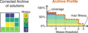
Figure 3. Illustration of the derivation of the Archive Profile (dashed orange line on the right) from a Corrected Archive (left). We also indicate how to retrieve the archive coverage and max fitness from the Archive Profile graph.

The Archive Profile is a holistic way of visualizing the fitness distribution of the resulting archive (Fontaine and Nikolaidis, 2021; Flageat et al., 2022b). More precisely, for a given fitness threshold $f_{\mbox{thres}}$, the Archive Profile corresponds to the number of archive cells $\mathcal{C}$ with a solution having a better expected fitness. In our experiments, we normalize it, by dividing the above quantity with the total number of cells. This way, we estimate the proportion of grid cells filled with solutions having a fitness greater than $f_{\mbox{thres}}$:

$$\textsc{ArchiveProfile}(f_{\mbox{thres}})=\frac{1}{N_{\mathcal{C}}}\sum_{\mbox{cell}\;\mathcal{C}}\varphi\left({f_{\mathcal{C}}\geq f_{\mbox{thres}}}\right)$$

where $\varphi\left({\cdot}\right)$ is the Iverson bracket, as described in section 4.1.3.

The Archive Profile exhibits several properties of interest for the archive. For instance its leftmost value on the $y$ axis corresponds to the archive’s total coverage; while the intersection of the curve with the $x$ axis indicates the highest fitness found in the archive (see Fig. 3 for an illustration).

4.2. Corrected Archives

The archives returned by QD algorithms may contain degenerate solutions, whose descriptor may significantly differ from the expected descriptor. Consequently, in such archives, the cell a solution is placed in may not be the cell of its expected descriptor; we designate those archives as: Illusory Archives. To alleviate this issue, our results are only presented in terms of Corrected Archive (Justesen et al., 2019; Flageat and Cully, 2020; Flageat et al., 2022b). Given an archive or set of genotypes returned by a QD algorithm, all genotypes are reevaluated $M$ times, and placed in a new archive, called ”Corrected Archive” based on their mean descriptor $\overline{{\bm{{d}}}}=\sum_{s=1}^{M}{\bm{{d}}}_{s}$; and in each cell, we only keep the solution having the best estimated expected fitness (see Formula 2). The main difference between an illusory archive and its corrected archive is depicted on Fig. 2.

Note that in this work, all the archive metrics detailed above are ”corrected” (Flageat et al., 2022b): they are only applied on the corrected archive. Consequently, we omit the prefix ”Corrected” when talking about the QD-Score, the NVS-Score and the P-Score.

4.3. ARIA Variants

Baseline	Reprod$\ast$	Fitness(es)	Descriptor
MOME-R	✓	$\begin{cases}\overline{f}=\frac{1}{N_{r}}\sum_{s=1}^{N_{r}}f_{s}\\ -\mbox{NDV}\end{cases}$	$\overline{{\bm{{d}}}}=\frac{1}{N_{r}}\sum_{s=1}^{N_{r}}{\bm{{d}}}_{s}$
ME-Sa-R	✓	$\overline{f}-NDV$$\ast\ast$	$\overline{{\bm{{d}}}}$
ME-Sa	✗	$\overline{f}$	$\overline{{\bm{{d}}}}$
MAP-Elites	✗	$f$	${\bm{{d}}}$

• Does the baseline optimize also for reproducibility?

• To get values of the same magnitude, the two terms are first normalized before being summed.

Table 1. Characteristics of the baselines under study.

ARIA can take as input any set of genotypes. As explained above, in ARIA, this set of genotypes goes through a Reproducibility Improvement phase, and is then used as a basis for finding new reproducible solutions in the rest of the archive. To study the effect of the initial set of genotypes, we initialize ARIA with different kinds of input. The corresponding variants are the following:

• ARIA- ME init which takes as input an archive returned by MAP-Elites. This way we initialize the ARIA algorithm with high-performing controllers that cover different areas of the descriptor space.

• ARIA- PGA init which takes as input an archive returned by PGA-ME (Nilsson and Cully, 2021). While this kind of environment is only compatible with QD-RL tasks (Tjanaka et al., 2022), it is expected to return better archives when the solutions parameterize high-dimensional deep-neural network controllers.

• ARIA- ES init runs an Evolution Strategy algorithm to maximize the performance of a single solution. The maximized objective is the expected fitness only; and we use the same optimization procedure as before (see section 2.1).

Also, we introduce a new variant, called ”Linear Reproducibility Improvement Mechanism” (Linear RIM), which does not optimize for the same objective function as ARIA. With this variant, we intend to show that the constraint-based objective function used by the Reproducibility Improvement Mechanism of ARIA is also of importance. In particular, the objective function used by Linear RIM is equal to the sum of the two (normalized) components of the objective function present in equation 1. The rest of the optimization procedure remains the same; and, similarly to ARIA- ME init, it takes as input an archive generated by MAP-Elites.

4.4. Baselines

The first baseline we consider for comparison with ARIA is the MAP-Elites algorithm, which samples only one descriptor and fitness per solution evaluation. This lower baseline does not take into account the uncertainty aspect of the problem. As a result, the illusory archive returned by MAP-Elites and its corresponding corrected archive may substantially differ (see Fig. 2).

We intend to also compare our variants of ARIA to several algorithms designed for Uncertain QD problems; these algorithms are detailed below, and their characteristics are summarized in Table 1.

• MAP-Elites Sampling (ME-Sa) (Justesen et al., 2019) works as MAP-Elites, except that for each solutions, it samples several fitnesses and descriptors, and use them to calculate the mean fitness and mean descriptor. This way, ME-Sa gets better estimates of a solution’s expected fitness and descriptor; and the archive returned by ME-Sa is expected to be more similar to its corrected archive.

• MAP-Elites Sampling with Reproducibility consideration (ME-Sa-R) is similar to ME-Sa, except that the fitness of each solution is modified to take into account the reproducibility problem. The fitness of ME-Sa-R adds a term that penalizes solutions having a high NDV score (see Table 1) on top of the expected task fitness.

• Multi-Objective MAP-Elites with Reproducibility consideration (MOME-R). As the problem to solve is initially a multi-objective problem (see Problem P1), we propose to also study the results obtained by a variant of Multi-Objective MAP-Elites (MOME) (Pierrot et al., 2022). The two fitnesses used by MOME-R are the two terms of the objective used by the ME-Sa-R baseline. We choose a Pareto front length of $50$, as in the introductory work of MOME. In this case, the MOME-R algorithm is not directly comparable to our approach, as the archive it returns may contain way more solutions than all other algorithms. Indeed, up to $50$ solutions may be stored in each cell of the MOME-R archive. To make this approach comparable, at analysis time, in each cell, we only pick the solution maximizing the ME-Sa-R objective (see Table 1).

4.5. Tasks

We compare the performance of all algorithms on three tasks, commonly used in Uncertain QD Settings (Flageat and Cully, 2023): the noisy 8 Degrees of Freedom (DoF) Arm, as well as the Ant Omni-directional and Walker Uni-directional Tasks.

4.5.1. Noisy 8-DoF Arm

The Arm task consists of a planar robotic Arm, that we control to reach different final positions (Cully and Demiris, 2018b). The solution consists of the angular positions of the successive actuators ${\bm{{\theta}}}=\left(\theta_{i}\right)_{i\in\left[1..8\right]}$. The fitness promotes solutions having an homogeneous set of angles, and some Gaussian noise is added to it to make its evaluations uncertain. Also, the descriptor corresponds to the final position $(x_{E},y_{E})$ of the end-effector perturbed by some Gaussian noise. The fitness and descriptor can be expressed as follows, with $\sigma_{f}=\sigma_{d}=0.01$:

(3) $$f({\bm{{\theta}}})=-\mbox{Var}\left({\theta_{i}}\right)+\mathcal{N}\left(0,\sigma_{f}^{2}\right)\quad{\bm{{d}}}({\bm{{\theta}}})=\begin{pmatrix}x_{E}\\ y_{E}\end{pmatrix}+\mathcal{N}\left({\bm{{0}}},\sigma_{d}^{2}{\bm{{I}}}\right)$$

4.5.2. Ant Omni-directional

The Ant Omni-directional task consists of finding high-dimensional controllers bringing a four-legged robot to diverse final positions. The task fits in the QD-RL setting (Tjanaka et al., 2022; Flageat et al., 2022b); it can be modeled as a Markov Decision Process (MDP), and the task fitness equals the non-discounted sum of rewards over an entire episode. In the case of the Ant Omni task, the reward promotes solutions who don’t die prematurely, while it penalizes high energy consumption $f=\sum_{t=1}^{T}r_{survive}-r_{energy}$ with $T=100$. Also, the descriptor corresponds to the final position of the robot: ${\bm{{d}}}=(x_{T},y_{T})$. We use the Ant Omni task as implemented in the QDax library (Lim et al., 2022), which itself relies on the Ant environment from Brax (Freeman et al., 2021). The learned controllers are closed-loop deep neural network policies, with two hidden layers of size 64, which output the torques to apply on the robot joints at each timestep. In this task, the noise is applied on the initial joint positions and velocities.

4.5.3. Walker Uni-directional

The Walker Uni-directional task consists of finding diverse ways to move forward as fast as possible. Similarly to the Ant Omni task, it fits in the QD-RL setting, and we also rely on the implementation from QDax using Brax. Furthermore, the noise and controllers considered are the same as for the Ant task. Nonetheless, the fitness and descriptor differ from the Ant task. Indeed, here the reward presents an additional term promoting forward displacement: $f=\sum_{t=1}^{T}r_{forward}+r_{survive}-r_{energy}$ with $T=1000$. The descriptor here characterizes the proportion of time each leg touches the ground: ${\bm{{d}}}=\frac{1}{T}\sum_{t=1}^{T}\left(C_{1}(t),C_{2}(t)\right)$, where $C_{i}(t)$ equals $1$ if leg $i$ touches the ground at timestep $t$, and equals $0$ otherwise.

4.6. Implementation Details

For each task under study, the descriptor space is two-dimensional, and is discretized in a $32\times 32$ grid. The archives given as input to ARIA- ME init and ARIA- PGA init are generated with respectively $2\,000\,000$ and $500\,000$ evaluations. At each iteration of the reproducibility improvement function, $N_{\mbox{s}}=2{,}048$ samples are generated for the Arm and Ant Omni tasks; and $N_{\mbox{s}}=1{,}440$ is chosen for the Walker task as it tends to be computationally heavier. We also use mirror sampling, so the Reproducibility Improvement Mechanism performs respectively $4{,}096$ and $2{,}880$ evaluations per iteration. Moreover, the samples are drawn with a standard deviation of $\sigma=0.005$, $0.02$ and $0.01$ respectively for the Arm, Ant and Walker tasks. Finally, the number of gradient steps taken by the reproducibility improvement mechanism is $N_{\mbox{grad}}=100$ for the Arm and Ant tasks; and $N_{\mbox{grad}}=75$ for the Walker task.

The MOME-R, ME-Sa-R and ME-Sa variants use a batch size of 128, with each solution reevaluated $N_{r}=32$ times, which makes a total sampling size (Flageat and Cully, 2023) of $4{,}096$ per iteration. Hence, we also use this value as batch size for the MAP-Elites baseline. All those baselines have a total budget equal to the maximal number of evaluations done by ARIA variants, i.e. $428\,228\,608$ for the Arm and Ant tasks, and $229\,386\,240$ for the Walker task.

At analysis time, each solution is reevaluated $M=1{,}024$ times to compute the archive profile. This value is used for all metrics.

All our implementation is based on the QDax framework (Lim et al., 2022), except for the reproducibility improvement mechanism, which is adapted from the evolution strategy implementation from Brax (Freeman et al., 2021). Each experiment was run on an NVIDIA RTX A6000; with this hardware, ARIA took respectively 20 minutes, 10 hours, and 18.5 hours to run the Arm, Ant and Walker tasks. We run each variant for 10 replications; and we evaluate the statistical significance of our comparisons using the Wilcoxon rank-sum test, with a Holm-Bonferroni correction (Holm, 1979). To facilitate the replications of the results, we stored our code and dependencies in a singularity container (Kurtzer et al., 2017), and made it available with the code at: https://bit.ly/aria-gecco.

5. Results

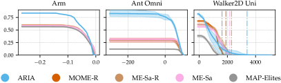
Figure 4. Archive Profiles of ARIA and other baselines. For clarity purposes, only one variant of ARIA is shown per plot. From left to right, the plotted variants of ARIA are respectively: ME init, ME init and PGA init. The bold line represents the median, and the shaded area corresponds to the inter-quartile range. The vertical lines on the Walker task represent the median max fitness.

Algorithm	Arm task			Ant Omni-directional task			Walker Uni-directional task
	QD-Score	V-Score	P-Score	QD-Score	V-Score	P-Score	QD-Score	V-Score	P-Score
ARIA - ME init	722.41	426.83	653.37	765.69	818.14	453.94	81.04	776.81	561.96
ARIA - PGA init	✗	✗	✗	679.06	756.64	414.12	180.72	839.87	634.06
ARIA - ES init	587.30	428.22	647.37	581.22	613.61	279.80	248.14	701.43	466.58
Linear RIM	704.68	394.23	542.58	610.28	619.30	341.06	115.13	642.80	373.22
MOME-R	538.62	303.57	258.03	287.90	268.79	47.77	175.75	692.74	284.29
ME-Sa-R	538.19	304.37	258.94	283.39	279.24	61.34	185.68	613.97	174.67
ME-Sa	534.06	301.37	253.61	307.26	251.20	33.40	168.70	554.26	123.61
MAP-Elites	506.34	288.63	318.59	117.91	93.65	13.44	66.87	357.52	19.75

Table 2. Median (Corrected) QD-Scores, Variance-Scores and Probability-Scores achieved by each algorithm on the three tasks under study. Note that the Arm task is not a QD-RL task (Tjanaka et al., 2022), so PGA-ME cannot be directly applied on it.

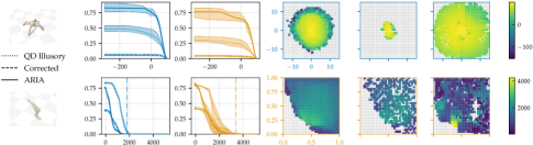
Figure 5. (columns 1 & 2) Archive Profiles of ARIA- ME init and ARIA- PGA init on the Ant and Walker tasks; (columns 3 to 5, from left to right) Illusory archive returned by the QD algorithm, its corresponding corrected archive, and the archive obtained after optimization from ARIA (the chosen archive is the one achieving the median QD-Score out of 10 replications). On the walker task, the vertical lines represent the median max fitness achieved by the archive returned by ARIA.

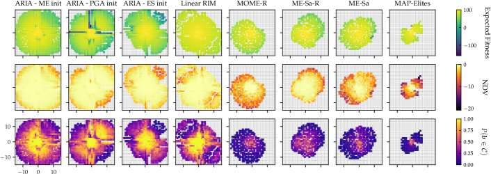
Figure 6. Distribution of the expected fitness, NDV score, and probability of belonging to cell in an archive returned by each algorithm, on the Ant Task. The chosen archive is the one achieving the median QD-Score out of 10 replications.

On the three tasks under study, ARIA improves substantially the archive profile of the corrected archive given by the initial QD algorithm. In particular, ARIA increases the coverage of the corrected archives by at least 50% on all tasks ($p<2\times 10^{-4}$, Figs. 2 and 5). Note that we do not intend to reach the results of the illusory archive, as this kind of archive contains many solutions whose evaluated fitness and descriptors differ substantially from their expected fitnesses and descriptors; hence nothing tells if such kind of archive is possible to obtain. Interestingly, on the Ant task, the coverage obtained by ARIA is even better than the coverage of the illusory archive ($p<2\times 10^{-4}$). It is also noticeable that on the Walker task, the corrected archive of ARIA-ME presents more individuals with a fitness higher than 900 compared to ARIA- ME init; this phenomenon may be due to the fact that ARIA optimizes for reproducibility before optimizing for performance, which is corroborated by its high Variance Score in Table 2 and by the extended analysis provided in Appendix C. Overall, these results demonstrate that ARIA improves not only the reproducibility of solution contained in any QD archive, but also can improve their content and sometimes their coverage. Videos of our results are available at: https://sites.google.com/view/gecco2023-aria/.

ARIA- ME init and ARIA- PGA init achieve a better reproducibility, i.e. higher V-Scores and P-Scores, than the other baselines which do not use a Reproducibility Improvement Mechanism (Table 2 and Fig. 6, $p<0.03$). This can be explained by the objective function that is explicitly maximized by ARIA, which puts the focus on the reproducibility before optimizing for the performance. Indeed, the objective introduced in section 3.3 prioritizes solutions that are in the cell compared to those that are not. Furthermore, the ES of the reproducibility improvement mechanism can scale to high-dimensional deep neural networks, making it easier for ARIA to explicitly optimize for reproducibility.

If we compare the results obtained by the various ARIA- ME init, we notice that the performance of each variant is correlated with its initialization. For example, on the ant task, the poor performance of the PGA initialization archive leads to low-quality results (Fig. 5). On the contrary, the ME init variant, which relies on a better corrected archive, manages to reach higher QD-Scores and archive coverage ($p<0.03$). Surprisingly, the ES init variant of ARIA achieves a better QD-score than its PGA counterpart (Table 2). However, on that task, the PGA initialization still manages to provide more reproducible archives, which is likely due to its internal optimization process as demonstrated in the literature (Nilsson and Cully, 2021; Flageat et al., 2022a).

In all tasks, the best QD-Score is obtained by a variant of ARIA (see Table 2), and their archive profiles exhibit a higher coverage (Fig. 4). Also, in the Walker task, the archive profile exhibits a higher maximal fitness. The worse QD Score obtained for some variants of ARIA (e.g. ES init on the Arm task and ME init on the Walker task) may be due to their initialization. Indeed, exploring from a single high-performing individual, as done by ARIA- ES init, may not be sufficient to find all the elites in the search space of the Arm task; and the high-dimensionality of the solutions in the Walker task prevents the ME initialization from finding high-performing individuals, which appears detrimental in the Walker task.

The constraint-based objective used by the Reproducibility Improvement mechanism is also of importance. Indeed, Linear RIM never manages to outperform ARIA-ME, both in terms of performance and reproducibility. On the Arm and Ant tasks, it achieves lower QD, Variance and Probability scores compared to ARIA-ME (Table 2, $p<8\times 10^{-3}$). On the Walker task, Linear RIM reaches a higher QD score compared to ARIA- ME init, but its Variance and Probability scores remain significantly lower ($p<2\times 10^{-4}$).

6. Discussion

In this work, we introduced ARIA, a plug-and-play algorithm designed to (1) enhance the performance and reproducibility of the solutions present in a QD archive, and (2) use those solutions to find new ones in the empty cells of the corrected archive. In the three tasks under study, we have shown that ARIA improves the overall performance, descriptor variance and coverage of corrected archives by a significant margin. We also demonstrate that ARIA can indifferently be applied on top of multiple QD algorithms.

However, our work has a few limitations. First, it requires a high number of evaluations; other optimization methods could be investigated to improve the sample-efficiency. Also, the way the cells are selected in the ”archive completion” phase could be improved; for now, the cells are selected without taking into account their solution’s performance or reproducibility. Finally, we only considered reproducibility with respect to the descriptor; it would be relevant to study how to also minimize the fitness variance.

Appendix A Mathematical Justifications

This section aims at providing mathematical proofs to justify the methods chosen in this paper.

Lemma 0.

If $(d^{(j)})$ refer to the components of a vector of random variables ${\bm{{d}}}$, then:

$$\sum_{j}\mbox{Var}\left[{d^{(j)}}\right]=\mbox{E}\left[{\left\lVert{\bm{{d}}}-\mbox{E}\left[{{\bm{{d}}}}\right]\right\rVert_{2}^{2}}\right]$$

Proof.

$$\mbox{E}\left[{\left\lVert{\bm{{d}}}-\mbox{E}\left[{{\bm{{d}}}}\right]\right\rVert_{2}^{2}}\right] =\mbox{E}\left[{\sum_{j}\left(d^{(j)}-\mbox{E}\left[{d^{(j)}}\right]\right)^{2}}\right]$$

$$=\sum_{j}\mbox{E}\left[{\left(d^{(j)}-\mbox{E}\left[{d^{(j)}}\right]\right)^{2}}\right]$$

$$=\sum_{j}\mbox{Var}\left[{d^{(j)}}\right]$$

∎

Theorem 2.

If we consider a bounded descriptor space, and a cell $\mathcal{C}$ such that $\mbox{E}\left[{{\bm{{d}}}}\right]\in\mathcal{C}$, then by maximizing the probability $\mbox{P}\left({{\bm{{d}}}\in\mathcal{C}}\right)$ in Problem P2, we minimize an upper bound on the sum of descriptor variances $\sum_{j}\mbox{Var}\left[{d^{(j)}}\right]$, which are present in Problem P1.

Proof.

By using Lemma 1, and then the law of total expectation, we get:

see Lemma 1 $$\sum_{j}\mbox{Var}\left[{d^{(j)}}\right] =\mbox{E}\left[{\left\lVert{\bm{{d}}}-\mbox{E}\left[{{\bm{{d}}}}\right]\right\rVert_{2}^{2}}\right]$$

$$=\mbox{E}\left[{\left\lVert{\bm{{d}}}-\mbox{E}\left[{{\bm{{d}}}}\right]\right\rVert_{2}^{2}|{\bm{{d}}}\in\mathcal{C}}\right]\mbox{P}\left({{\bm{{d}}}\in\mathcal{C}}\right)$$

$$\quad+\mbox{E}\left[{\left\lVert{\bm{{d}}}-\mbox{E}\left[{{\bm{{d}}}}\right]\right\rVert_{2}^{2}|{\bm{{d}}}\notin\mathcal{C}}\right]\mbox{P}\left({{\bm{{d}}}\notin\mathcal{C}}\right)$$

$$=\mbox{E}\left[{\left\lVert{\bm{{d}}}-\mbox{E}\left[{{\bm{{d}}}}\right]\right\rVert_{2}^{2}|{\bm{{d}}}\in\mathcal{C}}\right]\mbox{P}\left({{\bm{{d}}}\in\mathcal{C}}\right)$$

$$\quad+\mbox{E}\left[{\left\lVert{\bm{{d}}}-\mbox{E}\left[{{\bm{{d}}}}\right]\right\rVert_{2}^{2}|{\bm{{d}}}\notin\mathcal{C}}\right](1-\mbox{P}\left({{\bm{{d}}}\in\mathcal{C}}\right))$$

Also $\mbox{P}\left({{\bm{{d}}}\in\mathcal{C}}\right)\leq 1$. And if we write $d_{\mathcal{C}}$ the maximum between two points of the cell $\mathcal{C}$, then, as $\mbox{E}\left[{{\bm{{d}}}}\right]\in\mathcal{C}$, then:

$$\forall{\bm{{d}}}\in\mathcal{C}\;\left\lVert{\bm{{d}}}-\mbox{E}\left[{{\bm{{d}}}}\right]\right\rVert_{2}^{2}\leq d_{\mathcal{C}}^{2}$$

Thus:

$$\mbox{E}\left[{\left\lVert{\bm{{d}}}-\mbox{E}\left[{{\bm{{d}}}}\right]\right\rVert_{2}^{2}|{\bm{{d}}}\in\mathcal{C}}\right]\leq d_{\mathcal{C}}^{2}$$

Furthermore, the descriptor space is bounded, so, there exist a constant $\alpha$ such that

$$\mbox{E}\left[{\left\lVert{\bm{{d}}}-\mbox{E}\left[{{\bm{{d}}}}\right]\right\rVert_{2}^{2}|{\bm{{d}}}\notin\mathcal{C}}\right]\leq\alpha$$

In the end, we obtain the following inequality:

$$\sum_{j}\mbox{Var}\left[{d^{(j)}}\right] \leq d_{\mathcal{C}}^{2}+\alpha(1-\mbox{P}\left({{\bm{{d}}}\in\mathcal{C}}\right))$$

So, under the assumptions expressed in the theorem, by maximizing $\mbox{P}\left({{\bm{{d}}}\in\mathcal{C}}\right)$, we minimize an upper bound on the sum of descriptor variances.

∎

Theorem 3.

If the fitness function is bounded, then by maximizing the expectation of $\widetilde{o}_{\mathcal{C}}$, we also maximize a lower bound on the two objectives of Problem P2: $\mbox{P}\left({{\bm{{d}}}\in\mathcal{C}}\right)$ and the expected fitness $\mbox{E}\left[{f}\right]$.

Proof.

Using the law of total expectation, and the definition of $\widetilde{o}$ (see Equation 1):

$$\mbox{E}\left[{\widetilde{o}}\right] =\mbox{E}\left[{\widetilde{o}|{\bm{{d}}}\in\mathcal{C}}\right]\mbox{P}\left({{\bm{{d}}}\in\mathcal{C}}\right)$$

$$\quad+\mbox{E}\left[{\widetilde{o}|{\bm{{d}}}\notin\mathcal{C}}\right]\left(1-\mbox{P}\left({{\bm{{d}}}\in\mathcal{C}}\right)\right)$$

$$=\mbox{E}\left[{f|{\bm{{d}}}\in\mathcal{C}}\right]\mbox{P}\left({{\bm{{d}}}\in\mathcal{C}}\right)$$

$$\quad+\mbox{E}\left[{f_{min}-\left\lVert{\bm{{d}}}-{\bm{{c}}}\right\rVert_{2}|{\bm{{d}}}\notin\mathcal{C}}\right]\left(1-\mbox{P}\left({{\bm{{d}}}\in\mathcal{C}}\right)\right)$$

$$\geq\mbox{E}\left[{f|{\bm{{d}}}\in\mathcal{C}}\right]\mbox{P}\left({{\bm{{d}}}\in\mathcal{C}}\right)+f_{min}\left(1-\mbox{P}\left({{\bm{{d}}}\in\mathcal{C}}\right)\right)$$

$$\geq(\mbox{E}\left[{f|{\bm{{d}}}\in\mathcal{C}}\right]-f_{min})\mbox{P}\left({{\bm{{d}}}\in\mathcal{C}}\right)+f_{min}$$

Thus:

$$\mbox{P}\left({{\bm{{d}}}\in\mathcal{C}}\right) \geq\frac{\mbox{E}\left[{\widetilde{o}}\right]-f_{min}}{\mbox{E}\left[{f|{\bm{{d}}}\in\mathcal{C}}\right]-f_{min}}$$

$$\geq\frac{\mbox{E}\left[{\widetilde{o}}\right]-f_{min}}{f_{max}-f_{min}}$$

which means that by maximizing $\mbox{E}\left[{\widetilde{o}}\right]$, we maximize a lower bound on $\mbox{P}\left({{\bm{{d}}}\in\mathcal{C}}\right)$.

Also, if by using the law of total expectations on the expected fitness:

$$\mbox{E}\left[{f}\right] =\mbox{E}\left[{f|{\bm{{d}}}\in\mathcal{C}}\right]\mbox{P}\left({{\bm{{d}}}\in\mathcal{C}}\right)$$

$$\quad+\mbox{E}\left[{f|{\bm{{d}}}\notin\mathcal{C}}\right]\left(1-\mbox{P}\left({{\bm{{d}}}\in\mathcal{C}}\right)\right)$$

And in particular, we know that:

$$\mbox{E}\left[{f|{\bm{{d}}}\notin\mathcal{C}}\right]\geq\mbox{E}\left[{f_{min}-\left\lVert{\bm{{d}}}-{\bm{{c}}}\right\rVert_{2}|{\bm{{d}}}\notin\mathcal{C}}\right]$$

And we have shown above that:

$$\mbox{E}\left[{\widetilde{o}}\right] =\mbox{E}\left[{f|{\bm{{d}}}\in\mathcal{C}}\right]\mbox{P}\left({{\bm{{d}}}\in\mathcal{C}}\right)$$

$$\quad+\mbox{E}\left[{f_{min}-\left\lVert{\bm{{d}}}-{\bm{{c}}}\right\rVert_{2}|{\bm{{d}}}\notin\mathcal{C}}\right]\left(1-\mbox{P}\left({{\bm{{d}}}\in\mathcal{C}}\right)\right)$$

Thus:

$$\mbox{E}\left[{f}\right]\geq\mbox{E}\left[{\widetilde{o}}\right]$$

which means that by maximizing $\mbox{E}\left[{\widetilde{o}}\right]$, we maximize a lower bound on the expected fitness $\mbox{E}\left[{f}\right]$.

∎

Appendix B Archives

We provide on Figure 7 and Figure 8 visualizations of the archives returned by all algorithms respectively for the Arm and Walker tasks. These figures complete the visualizations provided in Figure 6 for the Ant task.

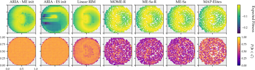
Figure 7. Distribution of the expected fitness, NDV score, and probability of belonging to cell in an archive returned by each algorithm on the Arm task. For each algorithm, the chosen archive is the one achieving the median QD-Score out of 10 replications. As the Arm task is not a QD-RL task, PGA-ME can not directly be applied on it. Also, the variance plots are not shown, as on the Arm task, all solutions have the same descriptor variance (see Formula 3).

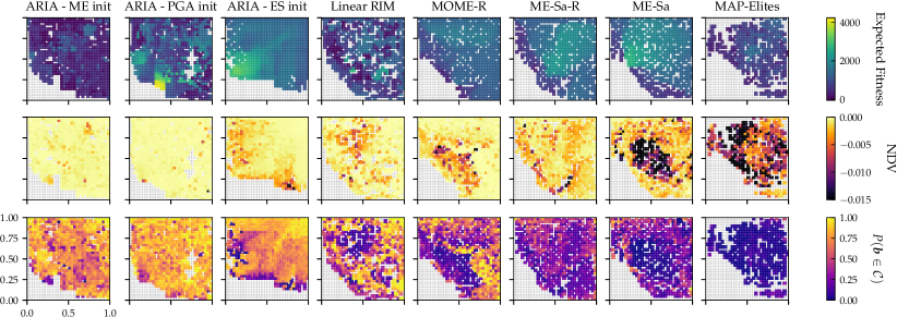
Figure 8. Distribution of the expected fitness, NDV score, and probability of belonging to cell in an archive returned by each algorithm on the Walker task. For each algorithm, the chosen archive is the one achieving the median QD-Score out of 10 replications.

Appendix C Walker Corrected Archive Analysis

We present on Figure 9, the Negative Descriptor Variance (NDV) scores and the probability values for the corrected archive and the ARIA- PGA init archive. We notice that the archive obtained by ARIA- PGA init loses some expected fitness in different cells. Nonetheless, ARIA- PGA init primarily optimizes the reproducibility before optimizing the performance (see Formula 1), and that is confirmed by the NDV and probability values in Figure 9. Interestingly, some holes appear on the ARIA- PGA init archive, at cells which were occupied in the Corrected Archive; this means the Reproducibility Improvement Mechanism may require some additional fine-tuning.

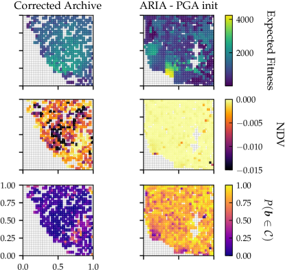
Figure 9. Distribution of the expected fitness, NDV score, and probability of belonging to cell for the corrected archive and ARIA- PGA init archive from the Walker Task on Figure 5.