Probing Conceptual Understanding of Large Visual-Language Models

Abstract

In recent years large visual-language (V+L) models have achieved great success in various downstream tasks. However, it is not well studied whether these models have a conceptual grasp of the visual content. In this work we focus on conceptual understanding of these large V+L models. To facilitate this study, we propose novel benchmarking datasets for probing three different aspects of content understanding, 1) relations, 2) composition and 3) context. Our probes are grounded in cognitive science and help determine if a V+L model can, for example, determine if “snow garnished with a man” is implausible, or if it can identify beach furniture by knowing it is located on a beach. We experimented with five different state-of-the-art V+L models and observe that these models mostly fail to demonstrate a conceptual understanding. This study reveals several interesting insights such as cross-attention helps learning conceptual understanding, and that CNNs are better with texture and patterns, while Transformers are better at color and shape. We further utilize some of these insights and propose a baseline for improving performance by a simple finetuning technique that rewards the three conceptual understanding measures with promising initial results. We believe that the proposed benchmarks will help the community assess and improve the conceptual understanding capabilities of large V+L models .

1 Introduction

Humans navigate the world by learning an “understanding” of how it works. Understanding may be defined as the underlying organization of all concepts including: objects, situations, events, and more [8, 25]. They are organized in our brains as conceptual maps, that encode structured, relational information [15]. Conceptual maps highlight major objects and actions in a system and the causal relations between them. While deep learning models have impressive performance in a variety of tasks, it is still unclear if their impressive performance is due to learnt conceptual maps.

Large visual-language (V+L) models are recently and greatly successful deep learning models that learn representations of image and text in a shared space. These representations are useful for downstream tasks like image classification, visual-question answering, image retrieval and more [52, 44, 32, 31, 47, 1]. However, for use in real-world applications, it is also vital that models “understand” rather than memorize to perform on more general tasks [29]. While large-language models have been shown to have a moderate amount of “theory of mind”, as measured by conceptual consistency [35], V+L models have not been investigated in a similar way using real-world examples. This is partly because images are more challenging as shown by preliminary studies [43, 11, 5]. With this in mind, we focus on probing models on their conceptual maps.

We develop a benchmark by combining insights from well known tests such as the Peabody Picture test with semantic analysis underpinning knowledge bases such as ConceptNet [40], and comprehension in elementary school education [35] to identify three key areas for probing: relations, composition and context. Our benchmark could be seen as a computational instantiation of visual comprehension testing along three important fundamental skills. These skills form a compact set of necessary, but not sufficient, prerequisites for key tasks such as concept transfer, analysis, evaluation and generation. They thus provide us a basis for probing comprehension of large V+L models.

We propose three benchmark datasets, Probe-R, Probe-A, and Probe-B, which focus on (1) object relationships to each other, (2) object’s relations to its attributes and (3) object’s relationships to its background context (Figure 1). Probe-R looks at model understanding of possible object relations by comparing an image to a correct prompt and an incorrect prompt where the predicate is swapped with an unlikely relation. If models are high performers in image-text matching, then they demonstrate an underlying understanding of what possible relationships can exist between certain objects. Probe-A looks at model understanding of possible attribute-object relations by comparing two images and two prompts where either the attribute is swapped with an antonym or the object is swapped. If models are high performers in this paired image-text matching, then they demonstrate an underlying understanding of what attribute assignments to objects looks like, and how to distinguish those visually. Finally, Probe-B looks at model understanding of objects and their relationships to their surroundings by removing background and observing the change in performance. If models are high performers in this image-text matching, then they demonstrate a lack of underlying understanding of what environments objects are most often appearing in, and with what other objects they are most often appearing with. While this is not a negative, it gives us insight into the underlying mechanisms of how these models may work, favoring object recognition instead of overall scene recognition.

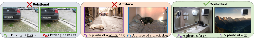
Figure 1: We present three datasets to evaluate V+L models on relational, compositional and contextual understanding. They utilize image-text matching tasks with predicate, object/subject, compositions, or background swaps. These examples are where CLIP is successful for contextual but not relational or compositional.

We experimented with five different state-of-the-art V+L models and provide several interesting insights regarding these models. For compositional understanding, we observe (1) Models struggle with compositionality (2) CNN based backbones may be better at recognizing texture and patterns while ViT backbones are better with color and shape. For relational understanding, we observe (1) both modality specific attention and co-attention in parallel improve relational understanding. (2) Predicate swapping that violates expectations surfaces the lack of an underlying conceptual model. For contextual understanding we observe that models tend to not use context in order to recognize most objects again indicating a lack of an underlying conceptual model. We further utilize these findings and propose a baseline by developing a simple finetuning approach based on selective negatives paradigm and observe improvement on our understanding-related probes at the expense of a slight loss in performance. In summary, we make the following contributions,

• We study the capability of existing large V+L models for complex visual perception focusing on relational, attribute and contextual understanding.

• We propose three benchmark datasets: Probe-R, Probe-A and Probe-B focusing on subject-object relations, attribute-object relations, and background-object relations.

• We exhaustively evaluate existing models and provide new insights about their capabilities such as the fact that cross-attention between modalities enables improvement in conceptual learning.

• We present a simple approach, based on prompting, that rewards compositionality and preservation of relations between objects, that yields more robust performance on our benchmarks.

2 Related Works

Several works have probed models to understand what models are learning [43, 11, 49, 28, 18]. The CLEVER dataset was designed to test models’ ability for visual reasoning by modifying the shape, size, texture, color and location of small objects in an isolated environment. Images are generated from a small set of possible combinations and are not from real-world examples. In Winoground [43], models were asked to match a pair of images to their correct caption from a pair, with challenging swaps in words. It showed that models performed worse than humans because it requires both compositional understanding and commonsense reasoning [11]. Without disentangling the individual skills required to perform well, it limits insights to why/how they are failing and where to improve. Another work focuses on visual perception of foreground versus background attention in images [26]. They asses visual models’ performance under different noise conditions (foreground, background, or no background). It also examined model salience by comparing attention values to ground truth segmentation. Of the 10 objects considered, they found for some (e.g. boat), models did attend to the background more than the object.

Some recent concurrent works have emerged in this area showing increasing interest from the community [24, 27, 19, 51]. In [50], CLIP [31] V+L models were evaluated on a small-scale benchmark based on Visual Genome [21] and MSCOCO [22]. Performance was defined as how well they could pick the correct order of subject, predicate and object triplets as well as attribute and object pairs. They found that models typically behave like bags-of-words and have little to no preference towards correctly ordered sentences. CREPE [24] swapped words, instead of changing order, with GPT-3 to generate natural language captions based on scene graphs of an image. They controlled for complexity based on the number of objects referenced. VL-Checklist [51] swapped words but also focuses on multiple categories of compositionality. When making swaps, they ensure similarity to the original caption to make the task more challenging and to asses model robustness. In contrast to other works, we utilize antonyms and unlikely relations to create hard negative prompts, augment images, and focus on visual comparisons. The goal of our benchmark is not necessarily accuracy when a slight change is made, but rather are models able to hold consistent understandings about what relations are possible between objects, and can they visually perceive relationships enough to apply these. Additionally, we probe models understanding and potential reliance on object co-occurrence and background-object co-occurrence.

Figure 2: Benchmark overview. Probe-R swaps the real subject or relation with an unlikely one and swaps a set of subject-only images to an subject-only prompt and the ground-truth relation prompt. Probe-A asks the model to match two images and two prompts, swapping object or composition. Probe-B compares object recognition performance before and after swapping out context from background and other surrounding objects.

3 Benchmark and Metrics

We evaluate three discrete concepts: object-relations, compositionality, and background context. We have generated three datasets: Probe-R, Probe-, and Probe-B. A summary of each dataset is shown in Figure 2 and Table 1. These benchmarks heavily rely on “prompting” the model by changing text input as well as image input in Probe-B. Prompting is typically done in downstream image classification by forming sentences with each class name in the prompt, such as “a photo of a dog”. The one with the highest similarity to the visual features is the predicted class [31, 39].

Table 1: A summary of proposed benchmark datasets. Groups refer to the group of images/text for each comparison being made. Under attributes, we list the dataset properties where fillers are the types of replacements we use when removing background pixels. Tasks include Image-Text matching (ITM), multi-label object recognition (MLR) and object recognition (R). See Figure 2 for illustrative examples of each group. Acc is for accuracy, $\gamma^{r}$ is the relative change in performance, mAP is mean-average-precision, and the group/image/text scores are accuracy based ITM metrics from [43].

Dataset	Task	Metric	Description	Source	Images	Group Description.	Groups	Attributes
Probe-R	ITM	Acc	Predicate/Object Swapping	Visual Genome	99,960	1 image, 10 pos.	99,960	2,456 Relations,
		Mean Softmax ($\mu(c)$)				images, 4 prompts		6,006 Objects
Probe-A	ITM	Group Score [43]	Attribute Swapping,	MSCOCO	40,681	2 images,	79,925	114 Attributes,
		Text/Image Score [43]	Object Swapping		59,205	2 prompts	375,607	2,462 Objects
Probe-B	MLR	mAP, $\gamma^{r}$	Background Removal,	MSCOCO	31,745	3 images,	31,745	4 fillers, 80 objects
	R	Acc, $\gamma^{r}$	Background+Object Removal		1,484	$\leq$80 prompts	9,375	4 fillers, 76 objects

Probe-R: Relational Understanding To generate a dataset that can be used to probe for relational understanding, we collected samples from the Visual Genome [21] dataset. The goal is to have high accuracy and confidence in selecting the correct prompt for the respective image where the incorrect prompt has either the relation or the object swapped. If the models have a greater understanding of what relationships are possible between a pair of objects, performance should be high. In summary, these samples are used to probe whether models have learned consistent concepts of objects and their potential relationships to each other. An overview of Probe-R is shown in Figure 2 and more details can be found in the Supplementary Section 1.1. For each group, we have four prompts $P\in\{R_{1},R_{2},R_{3},O_{1}\}$, one anchor image $X_{R_{1}}$ and 10 images $\mathbf{X}_{O_{1}}$ with the subject present and no other objects found in the anchor image. For each $X_{R_{1}}$, the ground truth relation $R_{1}=\langle s_{1},r_{1},o_{1}\rangle$ is compared to a swap of subject $R_{3}=\langle\overline{s}_{1},r_{1},o_{1}\rangle$ or predicate $R_{2}=\langle s_{1},\overline{r}_{1},o_{1}\rangle$. We sample $\overline{s}_{1}$ uniformly from subjects that do not occur in the dataset with $r_{1}$ and $o_{1}$ and similarly $\overline{r}_{1}$ is sampled uniformly from relations that do not occur with $s_{1}$ and $o_{1}$. This swapping of unlikely subjects and predicates allows us to test whether V+L models have learned consistent conceptual models of what object relations are possible in a system by comparing existing ones to unlikely ones. The final comparison is subject-only images $X_{O_{1}}$ to $P_{R_{1}}$ and a prompt with only the subject $P_{O_{1}}$. Table 1 summarizes the annotations in Probe-R.

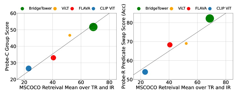
Figure 3: Reported MSCOCO retrieval scores (x-axis) against group score for Probe-A and Predicate Swap ($P_{R_{1}}\text{ vs }P_{R_{2}}$) accuracy in Probe-R (y-axis), there is a linear trend. This suggests that the MSCOCO retrieval is an indicator of performance on this benchmark. Circle size is based on model parameters and we do not see a linear trend.

Probe-A: Attribute Understanding To generate a dataset that can be used to probe for understanding, we collected samples from the MSCOCO Captions dataset [22]. These samples are used to probe whether models have learned an understanding of object attributes and their relationships to each other. An overview of Probe-A is shown in Figure 2 and additional details are in the Supplementary Section 1.2. The goal is to have high group accuracy, meaning that the model was able to match the correct prompts to the correct images where one attribute is compared to its antonym and the objects being described remain the same, or the object is different, but the attributes remain the same. If group accuracy is high, then models demonstrate greater understanding of what attribute assignment looks like for certain objects and are able to visually distinguish between them. For each group, we have two images $x_{1}$ and $x_{2}$ and two prompts $p_{1}$ and $p_{2}$. This dataset has two splits, one where the attributes are swapped in the prompts and the other where objects are swapped. When swapping attributes, antonyms were manually mapped to each attribute to ensure that the attribute is not present in the image. For example, if there is a “small dog” in an image, the comparison could be “a large dog”. When swapping objects, the images must have the same attribute but different objects. Table 1 shows a summary of Probe-A.

Probe-B: Contextual Understanding To generate a dataset that probes for model understanding on objects and their relationship to contextual cues found in an image’s background, we collected samples from MSCOCO [22] consisting of 80 objects. These samples are used to probe model reliance on background cues and reliance on co-occurrence between objects. An overview of Probe-B is shown in Figure 2 For each group, there is an unmodified image $x_{0}$, an image with a random patch on the background $\tilde{x_{0}}$, a modified image where the background is removed $\tilde{x_{1}}$ and 80 or less prompts. We have two splits in this data, the first removing the background but keeping all objects Probe-B_MR and the other removing both background and all other objects Probe-B_R. Probe-B_R aims to probe models on whether they use conceptual maps on object co-occurrence to improve recognition. Probe-B_MR aims to probe models on whether they have conceptual maps related to what group of objects are likely to be in what scenery or possible physical relations to each other. Poor performance on these tasks would indicate model use of such conceptual mappings, while good performance means they are focusing on object recognition only. We experiment with four fillers: black, gray, Gaussian noise, or a random scene. Random scenery was collected from the Indoor Scenes Dataset [30] and the Kaggle Landscape dataset [34]. These images were manually filtered to ensure none of the 80 MSCOCO classes were present. For single objects, images were only kept if the size of the object was between a threshold where the object was not too large and not too small relative to the image size. Table 1 shows a summary about the annotations in Probe-B.

3.1 Metrics

For each dataset we use different metrics that focus on change in model confidence following the psychological “violation-of-expectation” (VoE) paradigm [29, 2]. If V+Ls are learning valid conceptual models, then confidence should remain high when choosing between the correct prompt and the prompt that is violating expectations. For Probe-R, by probing models with data that is intended to violate expectation, we expect the confidence to remain high. For Probe-A, by probing models with paired opposites, we also expect the confidence to be high. For Probe-B, by removing visual information or replacing it with a violation of the original information, we expect the model to become confused and therefore the confidence to be low.

Probe-R Metrics When comparing an image to two prompts, or vice-versa, we measure mean confidence ($\mu(c)$) and accuracy (Acc). For Probe-R, we compare one image $x$ to two prompts $p_{1}$ and $p_{2}$. We convert two logit scores from model $f$ to softmax $\sigma$ predictions to measure the confidence $c_{1}$ of $p_{1}$ and $c_{2}$ of $p_{2}$. Using $c_{1}$ and $c_{2}$, we measure accuracy based on whether the confidence of the correct prompt is higher than the incorrect prompt. The metrics we present are the mean confidence $\mu(c)$ and mean accuracy (Acc) over all groups.

Probe-A Metrics To measure image and text matching between two images, $x_{1}$ and $x_{2}$, and two prompts, $p_{1}$ and $p_{2}$, using logit output from a model $f$, we adopt metrics from [43] measuring a text score, an image score and a group score. The text score ($t$) measures the accuracy of the model selecting the correct prompt for a given image: $f(p_{1},x_{1})>f(p_{2},x_{1})\text{ and }f(p_{2},x_{2})>f(p_{1},x_{2})$. The image score ($i$) is the reverse, measuring the accuracy of selecting the correct image given the prompts: $f(p_{1},x_{1})>f(p_{1},x_{2})\text{ and }f(p_{2},x_{2})>f(p_{2},x_{1})$. The group score ($g$) measures the accuracy of both combinations: $t(p_{1},x_{1},p_{2},x_{2})\text{ and }i(p_{1},x_{1},p_{2},x_{2})$.

Probe-B Metrics To measure performance for when just the background is removed, we look at average precision (mAP) of all objects in the image. For when other objects are also removed, we look at accuracy (Acc) compared to prompts for all objects but those that were present in the original image. To consider robustness to any changes to the original image, we randomly add a patch of the current filler that does not occlude any of the annotated objects. The compared images are the original image $x_{0}$, the patched image $\tilde{x_{0}}$, and the image with the background removed $\tilde{x_{1}}$. We collect the similarity between the image $x_{n}$ and for each object $o$ placed in a prompt $p_{o}\in\mathbf{p}$. This results in a set of similarity scores for each object prompt. When other objects are removed, we do not include prompts for those removed objects. We use these scores to measure the mean average precision (mAP) for multiple object recognition or accuracy for when only one object is present. The change in model confidence ($\triangledown c$) is measured by $f(x,p_{o})-f(\tilde{x},p_{o})$ and relative robustness ($\gamma^{r}$) is measured by $1-(h(x,\mathbf{p})-h(\tilde{x},\mathbf{p}))/h(x,\mathbf{p})$ where $h(\cdot)$ is either mAP or accuracy.

4 Benchmark Results

In this section we go through the models we are evaluating in this benchmark and then present the evaluation on the proposed datasets Probe-R, Probe-A and Probe-B.

Table 2: Summary of models used in this study. The pre-training datasets include MSCOCO [22], SBU Captions, Loc. Narratives (LN), Vis. Genome (VG) [21], Wiki Image Text (WIT) [41], Conceptual Captions (CC) [37], Conceptual Cap. 12M (CC12) [6], Red Caps (RC) [10], YFCC100M [42], and LAION-400M [36].

Model	Params	Datasets	Images	Captions	Architecture	Attention
CLIP RN50	102M	LAION-400M	400M	400M	dual-stream	modality-specific
CLIP RN101	121M	LAION-400M	400M	400M	dual-stream	modality-specific
CLIP ViT B16/32	150M	LAION-400M	400M	400M	dual-stream	modality-specific
CLIP ViT L14	428M	LAION-400M	400M	400M	dual-stream	modality-specific
FLAVA	358M	MSCOCO, SBU, LN, CC, CC12, VG, WIT, RC, YFCC100M	70M	70M	dual-stream	modality-specific, merged
ViLT	112M	MSCOCO,VG,SBU,CC	4.20M	9.58M	single-stream	modality-specific, merged
Bridgetower	865M	MSCOCO,VG,SBU,CC	4.20M	9.58M	dual-stream	modality-specific, co-attn, merged

Models We perform our experiments on four recently developed and publicly available models: CLIP [31], FLAVA [39], ViLT [20] and BridgeTower [47]. A summary of these models and their pre-training datasets are shown in Table 2. CLIP [31] is dual-stream, using independent, modality specific encoders which are aligned in the same space only because of a contrastive loss between text-image pairs. FLAVA [39] is also dual-stream, and uses encoders based on ViT [12]. It adds a multimodal encoder which merges the single streams and co-attends. It performs unimodal training followed by multimodal training on a global contrastive loss, a masked multimodal modeling task (MMM), and an image-text matching (ITM) loss. ViLT [20] is a single-stream transformer that uses co-attention between modalities. It concatenates word embeddings and linear projections of image patches as input to a pre-trained ViT [9, 12]. It trains using ITM, masked language modeling (MLM), and word-patch alignment losses. Bridgetower [47] uses a dual-stream encoder with an multimodal encoder that incorporates the single-stream encoders at multiple layers using cross-attention based “bridge layers”. It uses CLIP’s ViT visual encoder, RoBERTa [23] as text encoder, and is trained with MLM and ITM losses. In summary, CLIP does not use co-attention, FLAVA merges then co-attends, ViLT uses a single-stream co-attention architecture, and BridgeTower combines dual-stream, co-attention and merging between the modalities.

4.1 Relational Evaluation

The overall results for the relation evaluation benchmark are shown in Figure 4 where on the right it shows each model’s accuracy and mean confidence $\mu(c)$ for matching the prompt to the anchor image $X_{R_{1}}$. The left shows example cases where models fail or succeed at matching the correct prompt. Additional results are in the supplementary.

Models are good at image-text matching when the object is swapped and poorer when the relationship is swapped: Mean confidence ($\mu(c)$) for the correct prompt when comparing to the relation/predicate swapped prompt is low. This indicates the models are “confused” when the relation is switched to a highly unlikely alternative. Figure 4 (a) shows different models’ successes and failures for predicate swapping. When swapping objects, the object that is swapped $\overline{s}$ is one that is highly unlikely, making this task simple if the model has a consistent understanding of what relationships are possible. Model confidence is higher when the object is swapped versus when the predicate is swapped. This may indicate that models are less confused when the tasks is specific to object recognition, focusing more on objects rather than the relationships between them. This may additionally indicate they are not understanding prompts as a “whole” but rather parts to a whole.

Summary BridgeTower and ViLT’s performance indicates that co-attention is a method that can improve relational understanding. BridgeTower’s performance may indicate co-attention from the “bridge layers” are improving learnt concepts about object relationships. (1) This would indicate that both modality specific attention and co-attention together improve relational understanding. (2) When the predicate is swapped by something that violates expectation, the drop in confidence, regardless of accuracy, indicates that their performance may not be due to an underlying conceptual map. (3) When the subject is swapped, all models show better performance compared predicate swapping, indicating they are focusing on objects less-so than there relations to each other.

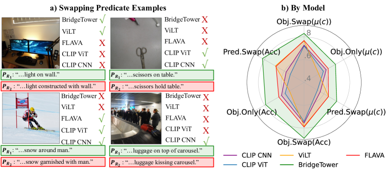
Figure 4: Probe-R. a) Examples of failure cases by model based on image-caption matching accuracy for Probe-R. b) Results for Probe-R where Pred.Swap is the anchor image $X_{R_{1}}$ compared to $P_{R_{1}}$ and $P_{R_{2}}$, Obj.Swap is the anchor image $X_{R_{1}}$ compared to $P_{R_{1}}$ and $P_{R_{3}}$, and Obj.Only is the object-only image $X_{R_{1}}$ compared to $P_{R_{1}}$ and $P_{O_{1}}$. The mean confidence $\mu(c)$ is the softmax score for the correct prompt to image. A table of results are shown in the Supplementary Table 1.

4.2 Attribute Evaluation

Overall results for evaluating model understanding of attribute-object relationships are shown in Figure 5 (c) with additional results in the Supplementary Table 2 and 3. We show the image, group and object scores as described in Section 3.1 for when the object is switched (Obj) and for when the attribute composition (Comp.) is switched.

Modality-specific attention and co-attention simultaneously greatly improves attribute-object relation understanding: When presented with two images and two captions where the attribute is the same but the objects are different, all models other than BridgeTower, perform on average double the performance versus when the attribute is switched. This discrepancy indicates typically models are relying more on object recognition when attributes are involved. BridgeTower’s high performance indicates further support that a combination of modality-specific attention and cross-attention in parallel improves the learning of underlying concepts.

Most models stronger with more physical attributes like “materials” as compared to visual-related like “color”: To better understand model failures when keeping the objects the same but swapping an attribute with its antonym, we categorized each attribute into 11 categories with results shown in Figure 5 (a). For example, “visibility” contains attributes like “dark” and “bright” while “expression” contains “smiley” and ”sad”. All models struggle when “visibility” related attributes. The best performance for non-CLIP models was within the “material” category with attributes such as “cloth” and “tin”.

Transformers and CNNs differ on which attributes they understand best: To compare backbone models, we average the image scores over CLIP backbone architectures in Figure 5 (b). Some noticeable patterns are that the CNN backbone models are better with “material”, “pattern” and “texture” related attributes while ViT’s are better at “color” and “shape”. This is similar to findings in [16] where they found ImageNet trained CNN’s are biased towards texture.

Summary (1) Models struggle with distinguishing between attributes but are better with those most associated with objects such as “materials”. (2) CNN based backbones may be better at recognizing texture and patterns while ViT backbones with color and shape. Surprisingly, (3) these models are typically better at matching captions given the image rather than text.

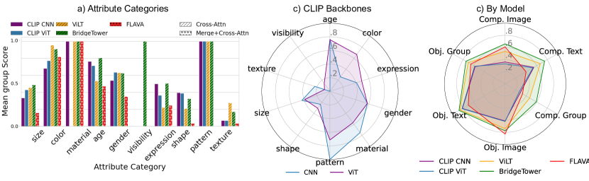
Figure 5: Probe-A. Mean group score a) averaged across attribute categories. b) We compare CLIP scores averaged over backbone. c) The overall results for Probe-A showing the image, text and group scores for when the object is swapped (Obj.) or when the attribute is swapped (Comp.). A table of results are shown in the Supplementary Table 2 and 3.

4.3 Background Context Evaluation

Overall results for evaluating model context understanding of background-object relationships are shown in Figure 7 and Figure 6. We evaluate model reliance on either background cues or the co-occurrence of objects. Both tasks compare to both an original image $x_{0}$ and the original image with an added patch of the respective filler $\tilde{x_{0}}$ to take into account general robustness. Modified images $\tilde{x_{1}}$ will have either the background removed and replaced with a filler or have the background and all other objects replaced. The fillers are one of: “black”, “gray”, “noise” or a random “scene” that does not have objects. The metrics we use for comparisons are the mean average precision (mAP) for multi-object recognition precision, relative robustness ($\gamma_{r}$) measuring the relative drop/increase in performance, and mean change in mAP $\mu(\triangledown(c))$ for the objects (see Section 3.1 for more details). Additional results can be found in the supplementary.

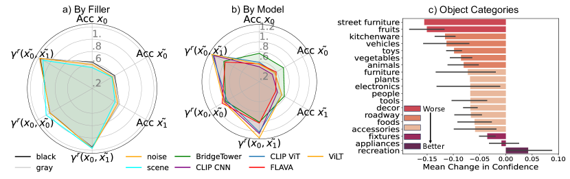
Figure 6: Probe-B removing background and all other objects. a) Results for when the background and all other objects are replaced with a filler $\tilde{x_{1}}$, compared to the original $x_{0}$, and original+random patch $\tilde{x_{0}}$. Metrics are object accuracy (Acc.) and the relative robustness $\gamma_{r}$. b) Mean change in confidence ($\mu(\triangledown c)$) from the ground truth $x_{0}$ to the modified $\tilde{x}_{1}$, where the background and other objects are removed. c) Mean change in confidence ($\mu(\triangledown c)$) from the ground truth $x_{0}$ to the modified $\tilde{x}_{1}$, where the background and other objects are removed. More details in Supplementary Table 6.

Models ignore what the background is replaced with, indicating little use of it: Figure 7 (b) shows the results averaged over filler type when only the background is removed. For all metrics, there is very little difference in performance. The most noticeable change is when comparing the ground truth image to $\tilde{x_{0}}$ and $\tilde{x_{1}}$ as expected. Overall, models are slightly less robust to when the background is replaced with either Gaussian noise or scenery. However, if models had underlying understanding of what objects belong in what context, models should be less robust to scenery. This indicates they may not have conceptual maps about objects and their relationship to context.

More co-attention may result in greater trade-off between robustness and performance: Figure 7 (b) shows the overall results averaged over model type when only the background is removed. Similar to when looking at fillers, models are typically robust to background removal, indicating little use of context. However, ViLT and BridgeTower tend to be less robust to when a patch is added to the image, noticeable even more so when the robustness between $\tilde{x_{0}}$ and $\tilde{x_{1}}$ is so high. This appears to be a trade-off between robustness and performance.

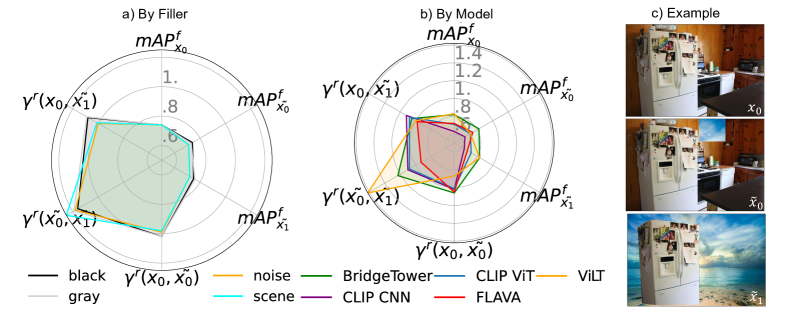
Figure 7: Probe-B removing background only. Mean results for replacing background with filler a) for each model averaged over fillers and b) for each filler averaged across models. Comparisons between the original $x_{0}$, original+random patch $\tilde{x_{0}}$ and modified $\tilde{x_{1}}$. The metrics are mAP and relative robustness ($\gamma_{r}$) When $\gamma_{r}>1$, the performance has improved. c) Sample images of what the dataset looks like for each variable. A table of results are shown in the Supplementary Table 7.

Some objects benefit from the presence of others, but most are better off without: Figure 6 shows the overall results for when the background and all other objects but one are removed, averaged over either filler (top) or model (bottom). When averaging over filler, models appear to be more robust when detecting one object as opposed to multiple objects in an image. When averaging scores over models, the robustness $\gamma^{r}$ tends to be over 1 when comparing to the background removed image $\tilde{x_{1}}$, indicating models improve when objects are in isolation. This indicates that models may be distracted from background information rather than using it for object recognition. In order to better understand what objects models are using background with more than others, we categorize objects into sub-categories as shown in Figure 6 (c). The object-types that models struggle with most appear to be large objects used in a common setting, such as “ovens” for appliances and “sink” for fixtures. This may indicate that there is some context used but for certain objects more than others.

Summary (1) Models tend to not use context in order to recognize multiple objects but (2) for some individual objects, models do use context. (3) These models are typically robust to a change in background where models like ViLT and BridgeTower are more susceptible to a particular patch being changed. (4) When objects are placed in random scenery that violates-expectation, models still perform similarly to when the original background is there, this may indicate that overall, models are not learning conceptual maps relating objects to their context.

5 Exploring finetuning for better conceptual understanding

Dual-stream encoders like CLIP and FLAVA allow uni-modal feature representations that can be extracted and used for a variety of downstream tasks. Improving models that do not require paired input would provide greater value and stronger representations. To establish a baseline for future work and explore this idea, we finetune (FT) CLIP on a new dataset inspired by this benchmark called RelComp. We propose using selective negative and positive pairing based on attribute and predicate swaps. We propose using two commonly used losses, an image-text matching (ITM) loss and a contrastive loss (C) [31, 39] (Figure 8). We curate a new dataset RelComp for attribute-object and object-object relations. This dataset is based on MSCOCO [22] and VisualGenome [21] and has no overlap between the benchmark datasets. We finetune CLIP ViT-B/32 using our proposed ITM and contrastive loss on RelComp. We linearly interpolate the original CLIP weights with our FT weights using an alpha$=0.2$ to prevent “catastrophic forgetting” [17, 46]. We call this “CLIP Patched” and finetune: visual-encoder only (V), text-encoder only (T) or both (VT). More details about losses, implementation and dataset are in the Supplementary.

Figure 8: Exploratory finetuning training scheme for CLIP. Image-text matching (ITM) is used as a triplet loss whose pairings vary depending on if it is a attribute assignment or a relational task. A contrastive loss is used to maintain general representations.

Table 3: Overall results for finetuning and patching the CLIP ViT-B/32 on the proposed RelComp dataset. ImageNet accuracy is shown to measure the drift from the original CLIP space. RelComp is the image score for the correct image-to-prompt matching. Probe-A/R are the mean accuracy for the correct image-prompt match. Top scores are in bold while second are underlined.

Model	ImageNet	RelComp	Probe-A	Probe-R
ViLT	–	76.00	90.78	69.00
BridgeTower	–	85.00	90.06	82.20
FLAVA	56.83	47.12	83.85	68.29
CLIP ViT B32	63.60	51.93	88.15	53.52
CLIP Patched (T)	57.85	67.85	89.49	71.14
CLIP Patched (V)	61.45	54.66	89.81	61.40
CLIP Patched (VT)	54.61	64.27	90.30	71.20

Overall results for our exploratory experiment are shown in Table 3. We observe drift in a trade off between visual recognition (ImageNet accuracy) and conceptual map understanding (Probe-A/R). When finetuning using the visual-encoder only, the drift is less pronounced, but so is the improvement on RelComp. The largest increase is seen with FT text encoder only. This may indicate that for non-cross-attention models, text is more important for conceptual mapping. Our findings indicate that by using selective negative sampling to enforce compositional and relational learning without extensive co-attention and computational complexity.

6 Conclusions

We evaluate large visual-language (V+L) models on relational, attribute and contextual understanding with three new datasets: Probe-A, Probe-R and Probe-B. Our benchmarking provides four key takeaways. Probe-R - Relations All models we tested are less sensitive to violations in expectations about relationships than about objects. Probe-A - Attributes Models have mostly accurate conceptual maps for some attributes (e.g., material descriptors) and poorer maps for others (e.g., visibility descriptors). Probe-B - Background Context Model performance is not noticeably impacted when removing the background and/or other objects. This shows little reliance on background cues for object recognition and poorer conceptual maps of context. Architectures Of the selected models, cross-attention and modality-specific simultaneously shows the greatest understanding based on these probes. Also, CNN backbones may be better at recognizing texture and patterns while ViT backbones are with color and shape.

In addition to these evaluations, we improved CLIP on these tasks by finetuning it on our proposed RelComp dataset, which was composed by selecting negatives. We found that (1) there is a small drop in classification performance, but (2) an improvement on Probe-R, Probe-A and RelComp is observed indicating an improvement in relational and compositional learning. We hope these insights will help drive future work on building V+L models that better “understand”.

Future Work While this benchmark focuses on image-text matching in V+L models, future can focus on Visual-Question Answering (VQA) and generative models. While we aim to establish a baseline of using selective word swaps to improve models’ understanding of compositionality, some concurrent works are already emerging exploring this idea further [50, 14, 13] showing improved success. We hope this benchmark and baseline can help researchers further these ideas in model understanding and compositionality. We hope this work can help drive future research in this area.

The supplementary will provide additional details about our proposed datasets, finetuning CLIP and the models evaluated on in this benchmark. Additional details and results for Probe-R, Probe-C and Probe-B are in Section A. We provide more details about finetuning CLIP and additional results in Section B. In Section D we provide additional details about the models we evaluated in this benchmark. Section G contains the Dataset Sheet for the proposed benchmarking datasets.

Appendix A Datasets Details

In this section we will provide additional results for the different dataset benchmarks. Dataset download, instructions, and details can be found at https://tinyurl.com/vlm-robustness.

A.1 Probe-R: Relational Understanding

This dataset was created using Visual Genome (VG) [21]. To collect unlikely “$<$subject, predicate, object$>$” triplets, we first cleaned the relationship aliases. This was done by mapping repeated aliases that meant the same thing into one, for example “are standing next to” would become “standing next to”. This was done to reduce the space to map all objects to aliases they have been associated with as well as to confirm they have not been associated with one similar. We then collect all the objects each cleaned alias was associated with using regex and NLTK part-of-speech (POS) tagging [3]. Using these object collections, we iterated through $100,000$ VG annotations of $R_{1}=\langle s_{1},r_{1},o_{1}\rangle$ to (1) replace the existing alias with an alias that the current subject and object are not associated with as swap ($R_{2}=\langle s_{1},\overline{r}_{1},o_{1}\rangle$) and (2) replace the existing subject with an object that is not associated with the current alias ($R_{3}=\langle\overline{s}_{1},r_{1},o_{1}\rangle$). To better collect images with specific objects in them, we iterated through VG and generated a mapping of each image ID to all objects present in the image according to the relationships annotations. We extract positive images $X_{O_{1}}$ that do not have the relation but have the subject and no other objects present in the anchor image $X_{R_{1}}$.

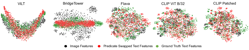
Figure 9: TSNE plots of image features (black) and text features from the Probe-R. Text features are prompts generated from either the ground truth relation $R_{1}$ (green) or the relation with the predicate swapped to an unrealistic one $R_{2}$ (red). Both ViLT and BridgeTower rely on cross-attention heavily, showing the impact on the feature space. While the features for the other models are more visibly in the same space, ViLT and BridgeTower generally show higher performance. CLIP patched is finetuning both visual and text encoders using RelComp and patching with an alpha of $0.2$ [17]. CLIP ViT is ViT/L-14@336px while CLIP CNN is RN50x4.

Model	$X_{R_{1}}$						$X_{O_{1}}$
	$P_{R_{1}}$ vs. $P_{R_{3}}$		$P_{R_{1}}$ vs. $P_{R_{2}}$		$P_{R_{1}}$ vs. $P_{O_{1}}$		$P_{R_{1}}$ vs. $P_{R_{2}}$
	$\mu(c)$	Acc	$\mu(c)$	Acc	$\mu(c)$	Acc	$\mu(c)$	Acc
CLIP RN50	$69.77$	$72.14$	$51.33$	$51.13$	$61.19$	$61.69$	$78.44$	$89.10$
CLIP ViT L/14	$71.59$	$73.68$	$52.44$	$52.59$	$59.09$	$58.67$	$84.17$	$93.23$
CLIP ViT-B/16	$71.08$	$73.40$	$52.84$	$53.37$	$61.69$	$62.07$	$79.62$	$89.96$
CLIP ViT/B-32	$69.00$	$71.21$	$53.02$	$53.53$	$58.83$	$58.56$	$82.21$	$92.32$
CLIP ViT	$72.09$	$74.27$	$53.52$	$53.97$	$59.53$	$59.14$	$83.97$	$93.50$
CLIP RN101	$70.62$	$73.28$	$54.01$	$55.11$	$60.66$	$60.83$	$79.08$	$91.17$
CLIP RN50x64	$72.79$	$74.79$	$56.66$	$58.03$	$64.10$	$64.88$	$78.10$	$87.15$
CLIP CNN	$72.71$	$75.59$	$56.35$	$58.14$	$62.31$	$62.81$	$78.29$	$90.77$
CLIP RN50x16	$73.91$	$76.57$	$58.08$	$60.52$	$59.80$	$59.79$	$83.03$	$94.05$
CLIP Patched (V)	$78.58$	$81.41$	$59.36$	$62.27$	$66.56$	$68.07$	$81.32$	$90.79$
FLAVA	$76.79$	$79.09$	$64.65$	$68.29$	$64.40$	$65.56$	$\underline{84.19}$	$90.12$
ViLT	$76.41$	$78.45$	$64.77$	$69.00$	$54.84$	$54.78$	$\mathbf{94.23}$	$\mathbf{99.10}$
CLIP Patched (VT)	$80.56$	$84.46$	$64.53$	$71.12$	$67.63$	$70.07$	$81.74$	$92.40$
CLIP Patched (T)	$\underline{82.37}$	$\underline{86.25}$	$\underline{66.28}$	$\underline{72.55}$	$\underline{67.93}$	$\underline{70.51}$	$79.76$	$90.70$
BridgeTower	$\mathbf{83.03}$	$\mathbf{89.01}$	$\mathbf{72.93}$	$\mathbf{82.04}$	$\mathbf{71.73}$	$\mathbf{78.90}$	$76.58$	$\underline{94.38}$

Table 4: Overall results for relation evaluation. The anchor image $X_{R_{1}}$ contains the relation $R_{1}=\langle s,r,o\rangle$, image $X_{O_{1}}$ contains $O_{1}=\langle s\rangle$. Prompts contain either the relation $P_{R_{1}}$, $P_{R_{2}}=\langle s,\overline{r},o\rangle$, $P_{R_{3}}=\langle\overline{s},r,o\rangle$, $P_{O_{1}}=\langle s\rangle$, or $P_{O_{3}}=\langle\overline{s}\rangle$. The mean confidence $\mu(c)$ is for the correct prompt to image. Models with CLIP Patched are those we finetuned on our training dataset RelComp. We finetuned either the text encoder (T), the visual encoder (V) or both (VT). Models show higher performance for when objects are switched but lower performance when the relation is switched, showing the models are confused.

	Composition Switch				Object Switch
Model	$\mu\left(c\right)\uparrow$	Image $\uparrow$	Text $\uparrow$	Group $\uparrow$	$\mu\left(c\right)\uparrow$	Image $\uparrow$	Text $\uparrow$	Group $\uparrow$
CLIP ViT	$69.69$	$33.06$	$52.82$	$26.64$	$88.15$	$61.96$	$81.89$	$58.05$
CLIP RN50	$69.47$	$33.41$	$54.60$	$26.92$	$87.00$	$61.40$	$80.17$	$56.81$
CLIP ViT-B/16	$69.23$	$34.29$	$52.23$	$26.94$	$88.02$	$63.53$	$81.44$	$59.12$
CLIP ViT L/14	$69.41$	$33.73$	$52.36$	$27.01$	$87.89$	$61.93$	$81.31$	$57.86$
CLIP RN101	$69.24$	$34.95$	$51.82$	$27.42$	$86.99$	$61.75$	$80.58$	$57.46$
CLIP RN50x64	$70.44$	$35.21$	$52.89$	$27.95$	$87.75$	$63.09$	$80.55$	$58.27$
CLIP ViT/B-32	$69.79$	$34.71$	$53.85$	$27.96$	$87.75$	$62.01$	$80.92$	$57.65$
CLIP RN50x16	$69.77$	$35.51$	$53.24$	$28.07$	$87.91$	$63.12$	$82.23$	$59.38$
CLIP CNN	$69.75$	$36.07$	$54.56$	$28.79$	$87.24$	$61.29$	$81.24$	$57.06$
FLAVA	$67.45$	$\underline{60.93}$	$39.65$	$33.09$	$83.85$	$\mathbf{82.66}$	$70.08$	$65.37$
CLIP Patched (T)	$71.94$	$40.96$	$58.79$	$33.83$	$89.58$	$68.81$	$84.36$	$65.19$
CLIP Patched (V)	$73.65$	$42.30$	$59.10$	$34.48$	$89.79$	$66.17$	$84.00$	$62.45$
CLIP Patched (VT)	$73.65$	$44.53$	$61.92$	$37.18$	$\underline{90.30}$	$70.01$	$85.41$	$66.83$
ViLT	$\underline{79.02}$	$53.74$	$\underline{66.84}$	$\underline{46.65}$	$\mathbf{90.78}$	$73.82$	$\underline{85.88}$	$\underline{70.26}$
BridgeTower	$\mathbf{81.88}$	$\mathbf{65.95}$	$\mathbf{75.02}$	$\mathbf{59.28}$	$90.05$	$\underline{77.44}$	$\mathbf{87.63}$	$\mathbf{74.54}$

Table 5: Overall results for the compositional evaluation on select models with highest scores in bold and second highest underlined. Mean confidence for the correct prompt-to-image is $\mu\left(c\right)$. CLIP ViT is ViT/L-14@336px while CLIP CNN is RN50x4.

Attribute	Category	Groups
age	[young, old, new]	2,051
color	[greyscale, coloured, sepia, reddish, bronze, greenish, green, turquoise, blue, tan, red, white, silver, purple, gold, pink, navy, brown, teal, gray, black, yellow, grey, golden, camo, pinkish, beige, orange, blonde]	39,971
expression	[happy, unhappy, smiling, laughing, smiley, sad]	2,088
gender	[male, female]	2,346
material	[tin, aluminum, cloth, gravel, unpaved, wooden, stainless, marble, metallic, metal, grassy, porcelain, wooded, pebbled]	3,875
pattern	[checkered, patterned, striped, spotted, plaid, stripped, checkerboard]	3,08
shape	[triangular, flat, circular, triangle, oval, round, dotted, rectangular, square]	1,164
size	[bulky, long, thin, large, big, tall, short, small, huge, tiny, giant, little, chubby, pudgy]	16,575
texture	[smooth, fluffy, fuzzy, dry, wet, rusty, bald, hairy, stony]	1,090
visibility	[shiny, unclear, sun, nightime, blurry, shadowy, lit, shady, light, darkened, hazy, dark, barren, cloudy, clear, sunlit, bright, foggy, rainy, sparkling]	10,454

Table 6: The attributes that belong to each category for the compositional analysis on specific attributes in Probe-C.

Model	age			color			expression			gender			material
	Image	Text	Group	Image	Text	Group	Image	Text	Group	Image	Text	Group	Image	Text	Group
CLIP RN50	$47.74$	$68.84$	$39.20$	$18.18$	$13.64$	$0.00$	$21.07$	$35.45$	$13.14$	$34.71$	$60.75$	$30.18$	$0.00$	$0.00$	$0.00$
CLIP RN50x64	$53.77$	$\underline{82.41}$	$49.25$	$4.55$	$13.64$	$0.00$	$20.08$	$36.28$	$13.97$	$39.64$	$\mathbf{70.61}$	$36.29$	$100.00$	$100.00$	$100.00$
CLIP RN101	$48.74$	$70.35$	$39.20$	$18.18$	$63.64$	$18.18$	$\underline{37.60}$	$43.97$	$24.30$	$32.35$	$55.23$	$27.02$	$0.00$	$100.00$	$0.00$
CLIP ViT	$53.27$	$71.36$	$46.73$	$18.18$	$77.27$	$18.18$	$20.91$	$38.26$	$15.62$	$45.17$	$69.03$	$40.43$	$100.00$	$0.00$	$0.00$
CLIP ViT-B/16	$45.73$	$76.88$	$40.70$	$27.27$	$77.27$	$22.73$	$28.84$	$\mathbf{66.94}$	$24.05$	$41.03$	$62.92$	$35.90$	$0.00$	$0.00$	$0.00$
CLIP ViT L/14	$53.77$	$75.88$	$47.74$	$31.82$	$72.73$	$27.27$	$18.43$	$16.28$	$11.82$	$41.62$	$\underline{69.43}$	$37.67$	$100.00$	$0.00$	$0.00$
CLIP CNN	$57.29$	$76.38$	$\underline{49.75}$	$31.82$	$68.18$	$31.82$	$25.21$	$47.93$	$19.01$	$37.67$	$56.80$	$30.77$	$0.00$	$\underline{100.00}$	$0.00$
CLIP Patched (T)	$41.71$	$79.40$	$37.69$	$31.82$	$68.18$	$31.82$	$37.27$	$\underline{61.98}$	$\mathbf{31.74}$	$46.94$	$54.83$	$36.09$	$100.00$	$100.00$	$\underline{100.00}$
CLIP ViT/B-32	$40.20$	$74.37$	$35.68$	$18.18$	$13.64$	$4.55$	$23.22$	$58.02$	$20.08$	$39.05$	$60.75$	$33.93$	$100.00$	$100.00$	$100.00$
CLIP Patched (V)	$44.72$	$76.38$	$39.70$	$40.91$	$\underline{90.91}$	$40.91$	$31.65$	$60.74$	$27.19$	$53.06$	$60.16$	$43.20$	$100.00$	$100.00$	$100.00$
CLIP Patched (VT)	$48.74$	$72.86$	$42.21$	$50.00$	$81.82$	$40.91$	$34.55$	$61.57$	$\underline{29.67}$	$52.47$	$57.00$	$42.60$	$\underline{100.00}$	$0.00$	$0.00$
FLAVA	$\mathbf{73.87}$	$47.24$	$43.22$	$86.36$	$81.82$	$68.18$	$\mathbf{39.67}$	$24.88$	$10.33$	$\mathbf{65.09}$	$42.60$	$37.67$	$100.00$	$100.00$	$100.00$
CLIP RN50x16	$52.76$	$\mathbf{83.92}$	$49.75$	$9.09$	$13.64$	$9.09$	$21.98$	$42.98$	$14.71$	$40.83$	$62.72$	$35.11$	$100.00$	$100.00$	$100.00$
BridgeTower	$\underline{68.34}$	$80.40$	$\mathbf{65.33}$	$\mathbf{95.45}$	$90.91$	$\mathbf{90.91}$	$32.23$	$52.07$	$24.79$	$\underline{57.79}$	$64.89$	$\underline{49.90}$	$100.00$	$100.00$	$100.00$
ViLT	$38.19$	$53.27$	$28.64$	$\underline{90.91}$	$\mathbf{95.45}$	$\underline{86.36}$	$4.79$	$18.43$	$1.57$	$57.59$	$67.46$	$\mathbf{51.28}$	$\mathbf{100.00}$	$\mathbf{100.00}$	$\mathbf{100.00}$
Model	pattern			shape			size			texture			visibility
	Image	Text	Group	Image	Text	Group	Image	Text	Group	Image	Text	Group	Image	Text	Group
CLIP RN50	$100.00$	$100.00$	$100.00$	$3.69$	$23.88$	$2.56$	$21.21$	$47.95$	$17.11$	$0.00$	$20.69$	$0.00$	$0.00$	$0.00$	$0.00$
CLIP RN50x64	$100.00$	$100.00$	$100.00$	$9.46$	$22.92$	$6.25$	$18.83$	$33.40$	$12.37$	$3.45$	$20.69$	$0.00$	$0.00$	$0.00$	$0.00$
CLIP RN101	$100.00$	$100.00$	$100.00$	$9.13$	$27.88$	$5.45$	$20.96$	$37.63$	$12.72$	$3.45$	$\mathbf{31.03}$	$3.45$	$50.00$	$0.00$	$0.00$
CLIP ViT	$100.00$	$100.00$	$100.00$	$10.26$	$\underline{38.94}$	$6.41$	$24.13$	$42.98$	$18.85$	$\underline{6.90}$	$6.90$	$0.00$	$50.00$	$0.00$	$0.00$
CLIP ViT-B/16	$0.00$	$100.00$	$0.00$	$8.01$	$21.63$	$3.21$	$15.69$	$28.33$	$7.73$	$6.90$	$17.24$	$0.00$	$\mathbf{100.00}$	$0.00$	$0.00$
CLIP ViT L/14	$0.00$	$100.00$	$0.00$	$\underline{13.46}$	$37.02$	$\underline{8.49}$	$24.84$	$45.11$	$\underline{19.34}$	$3.45$	$6.90$	$0.00$	$50.00$	$0.00$	$0.00$
CLIP CNN	$\underline{100.00}$	$\underline{100.00}$	$\underline{100.00}$	$12.82$	$\mathbf{39.58}$	$\mathbf{8.81}$	$17.51$	$33.43$	$10.62$	$0.00$	$6.90$	$0.00$	$0.00$	$0.00$	$0.00$
CLIP Patched (T)	$0.00$	$0.00$	$0.00$	$6.25$	$22.92$	$3.04$	$20.40$	$43.08$	$16.09$	$3.45$	$10.34$	$0.00$	$50.00$	$50.00$	$0.00$
CLIP ViT/B-32	$0.00$	$0.00$	$0.00$	$7.85$	$26.60$	$4.97$	$13.63$	$34.47$	$7.05$	$0.00$	$3.45$	$0.00$	$50.00$	$0.00$	$0.00$
CLIP Patched (V)	$0.00$	$100.00$	$0.00$	$10.10$	$28.04$	$6.41$	$16.29$	$44.60$	$10.42$	$0.00$	$6.90$	$0.00$	$\underline{50.00}$	$\underline{50.00}$	$\mathbf{50.00}$
CLIP Patched (VT)	$0.00$	$0.00$	$0.00$	$7.37$	$23.24$	$5.45$	$25.14$	$45.67$	$17.03$	$3.45$	$\underline{27.59}$	$3.45$	$0.00$	$50.00$	$0.00$
FLAVA	$0.00$	$0.00$	$0.00$	$\mathbf{34.62}$	$3.37$	$2.72$	$\mathbf{48.66}$	$16.09$	$12.60$	$\mathbf{31.03}$	$3.45$	$\underline{3.45}$	$0.00$	$0.00$	$0.00$
CLIP RN50x16	$\mathbf{100.00}$	$100.00$	$\mathbf{100.00}$	$7.85$	$19.87$	$4.49$	$22.93$	$\mathbf{54.13}$	$18.88$	$3.45$	$20.69$	$0.00$	$0.00$	$0.00$	$0.00$
BridgeTower	$100.00$	$100.00$	$100.00$	$7.53$	$32.53$	$6.41$	$\underline{25.54}$	$\underline{49.06}$	$\mathbf{20.40}$	$0.00$	$17.24$	$0.00$	$0.00$	$\mathbf{100.00}$	$0.00$
ViLT	$0.00$	$\mathbf{100.00}$	$0.00$	$5.13$	$20.99$	$2.56$	$17.44$	$45.36$	$14.75$	$6.90$	$27.59$	$\mathbf{3.45}$	$0.00$	$0.00$	$\underline{0.00}$

Table 7: Mean image, text and group scores for each category of attributes for each model.

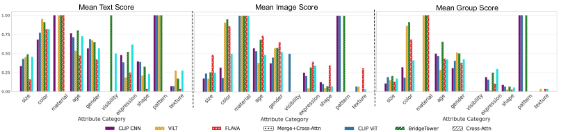
Figure 10: Mean image, text and group scores for a subset of models. Models are typically better matching a caption given an image rather than the reverse.

Object	Category	Groups
accessories	[backpack, umbrella, handbag, tie, suitcase]	174
animals	[bird, cat, dog, horse, sheep, cow, elephant, bear, zebra, giraffe]	627
appliances	[microwave, oven, toaster, refrigerator]	591
decor	[clock, vase]	138
electronics	[tv, laptop, mouse, remote, keyboard, cell phone]	1095
fixtures	[toilet, sink]	387
foods	[sandwich, hot dog, pizza, donut, cake]	258
fruits	[banana, orange]	120
furniture	[chair, couch, bed, dining table]	546
kitchenware	[bottle, wine glass, cup, fork, knife, spoon, bowl]	399
people	[person]	720
plants	[potted plant]	108
recreation	[frisbee, skis, snowboard, sports ball, kite, baseball bat, baseball glove, skateboard, surfboard, tennis racket]	117
roadway	[traffic light, fire hydrant, stop sign, parking meter]	144
street furniture	[bench]	42
tools	[scissors, hair drier, toothbrush]	15
toys	[book, teddy bear]	144
vegetables	[broccoli, carrot]	111
vehicles	[bicycle, car, motorcycle, airplane, bus, train, truck, boat]	603

Table 8: The objects that belong to each category for the object-context analysis on specific objects in Probe-B.

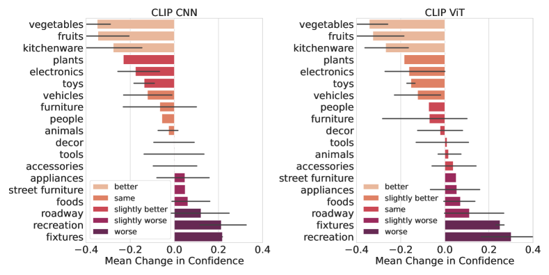
Figure 11: Comparing the change in confidence from a patched image $\tilde{x_{0}}$ to the image where all other objects and background $\tilde{x_{1}}$ is removed aggregated over CLIP backbones.

	Average Precision (mAP)			Relative Robustness ($\gamma_{r}$)			Mean Change Confidence ($\mu(\triangledown(c)$)
Filler	$x_{0}$	$\tilde{x_{0}}$	$\tilde{x_{1}}$	$(x_{0},\tilde{x_{1}})$	$(x_{0},\tilde{x_{0}})$	$(\tilde{x_{0}},\tilde{x_{1}})$	$(c_{0}-\tilde{c_{0}})$	$(\tilde{c_{0}}-\tilde{c_{1}})$	$(c_{0}-\tilde{c_{1}})$
black	$74.24$	$\mathbf{73.57}$	$\underline{75.28}$	$\underline{1.08}$	$\mathbf{1.02}$	$1.16$	$\underline{0.81}$	$\mathbf{-0.80}$	$\mathbf{0.01}$
noise	$\underline{74.37}$	$71.38$	$71.76$	$1.00$	$0.99$	$1.18$	$2.08$	$-0.62$	$1.46$
gray	$\mathbf{74.38}$	$\underline{73.47}$	$\mathbf{75.96}$	$\mathbf{1.09}$	$\underline{1.02}$	$\underline{1.19}$	$\mathbf{0.95}$	$\underline{-0.98}$	$\underline{-0.03}$
scene	$74.34$	$71.36$	$71.71$	$1.01$	$0.99$	$\mathbf{1.25}$	$1.81$	$-0.69$	$1.12$
Model	$x_{0}$	$\tilde{x_{0}}$	$\tilde{x_{1}}$	$(x_{0},\tilde{x_{1}})$	$(x_{0},\tilde{x_{0}})$	$(\tilde{x_{0}},\tilde{x_{1}})$	$(c_{0}-\tilde{c_{0}})$	$(\tilde{c_{0}}-\tilde{c_{1}})$	$(c_{0}-\tilde{c_{1}})$
CLIP RN50	$65.05$	$65.47$	$60.30$	$1.00$	$1.02$	$0.99$	$\underline{-0.05}$	$4.86$	$4.82$
CLIP ViT/B-32	$68.77$	$67.49$	$61.10$	$0.95$	$0.99$	$0.98$	$0.40$	$5.12$	$5.52$
CLIP CNN	$63.23$	$63.56$	$63.46$	$\mathbf{1.12}$	$1.02$	$1.10$	$0.46$	$2.64$	$3.11$
CLIP RN101	$64.56$	$65.00$	$63.80$	$\underline{1.09}$	$1.02$	$1.08$	$0.21$	$2.79$	$3.00$
CLIP ViT-B/16	$69.97$	$68.54$	$65.15$	$0.99$	$0.98$	$1.02$	$0.36$	$2.92$	$3.28$
FLAVA	$72.05$	$\underline{74.47}$	$66.75$	$0.98$	$\underline{1.05}$	$0.94$	$0.00$	$0.01$	$\underline{0.01}$
CLIP ViT L/14	$70.98$	$69.38$	$68.99$	$1.04$	$0.98$	$1.08$	$0.94$	$1.17$	$2.12$
CLIP ViT	$71.05$	$70.94$	$71.50$	$1.08$	$1.01$	$1.08$	$0.70$	$0.52$	$1.22$
ViLT	$\mathbf{83.49}$	$71.38$	$\underline{83.26}$	$1.00$	$0.87$	$\mathbf{1.62}$	$6.68$	$\mathbf{-6.61}$	$0.08$
BridgeTower	$\underline{81.85}$	$\mathbf{81.88}$	$\mathbf{83.40}$	$1.05$	$\mathbf{1.06}$	$\underline{1.23}$	$\mathbf{-0.79}$	$\underline{-0.42}$	$\mathbf{-1.22}$

Table 9: Mean results for Probe-$B_{R}$ when the background of an image is replaced with each filler (top) and for each model averaged over fillers (bottom). Comparisons are between the original image $x_{0}$, original image with a random patch $\tilde{x_{0}}$ and the modified image $\tilde{x_{1}}$ where the background is removed. The metrics are mean average precision (mAP), relative robustness ($\gamma_{r}$) measuring the relative drop/increase in performance, and mean change in softmax confidence $\mu(\triangledown(c))$ for the objects.

	Accuracy			Relative Robustness $\gamma^{r}$
Filler	$x_{0}$	$\tilde{x_{0}}$	$\tilde{x_{1}}$	$(x_{0},\tilde{x_{1}})$	$(x_{0},\tilde{x_{0}})$	$(\tilde{x_{0}},\tilde{x_{1}})$
noise	$54.26$	$53.58$	$63.07$	$1.17$	$\underline{0.99}$	$1.18$
scene	$49.85$	$53.41$	$58.15$	$1.17$	$\mathbf{1.08}$	$1.09$
black	$\underline{56.80}$	$\mathbf{55.74}$	$\underline{68.02}$	$\underline{1.21}$	$0.98$	$\underline{1.23}$
gray	$\mathbf{57.24}$	$\underline{55.28}$	$\mathbf{68.40}$	$\mathbf{1.21}$	$0.97$	$\mathbf{1.25}$
Model	$x_{0}$	$\tilde{x_{0}}$	$\tilde{x_{1}}$	$(x_{0},\tilde{x_{1}})$	$(x_{0},\tilde{x_{0}})$	$(\tilde{x_{0}},\tilde{x_{1}})$
BridgeTower	$\mathbf{77.36}$	$\mathbf{76.14}$	$\mathbf{77.70}$	$1.01$	$0.98$	$1.02$
FLAVA	$56.33$	$\underline{59.16}$	$58.32$	$1.03$	$1.06$	$0.99$
CLIP ViT/B-32	$46.19$	$50.50$	$54.20$	$1.17$	$\mathbf{1.10}$	$1.07$
CLIP ViT-B/16	$51.12$	$51.31$	$60.30$	$1.18$	$1.01$	$1.17$
CLIP ViT L/14	$56.27$	$54.18$	$67.16$	$1.19$	$0.96$	$1.24$
CLIP RN50	$45.79$	$48.64$	$55.68$	$1.21$	$\underline{1.07}$	$1.14$
CLIP ViT	$\underline{59.31}$	$56.08$	$71.76$	$1.21$	$0.95$	$1.28$
CLIP RN101	$46.48$	$47.92$	$57.32$	$1.23$	$1.03$	$1.20$
CLIP RN50x16	$53.88$	$50.92$	$66.18$	$1.23$	$0.95$	$\underline{1.30}$
CLIP RN50x64	$56.86$	$53.70$	$70.04$	$1.23$	$0.95$	$1.30$
CLIP CNN	$50.08$	$49.66$	$62.18$	$\underline{1.24}$	$1.00$	$1.25$
ViLT	$54.73$	$55.82$	$\underline{72.09}$	$\mathbf{1.33}$	$1.02$	$\mathbf{1.30}$

Table 10: Results for when the background and all other objects are replaced with a filler $\tilde{x_{1}}$, compared to the original image $x_{0}$, and an image with a random patch of the same filler type $\tilde{x_{0}}$. Metrics used are the accuracy of detecting the object compared to other objects that are not present in the image and the relative robustness $\gamma_{r}$, which is the relative change in confidence.

		RelComp			ImageNet
Stream	alpha	Group Score	Image Score	Text Score	Top1	Top5
v	0.2	$31.52$	$54.67$	$53.17$	$\mathbf{61.45}$	$\mathbf{87.73}$
v	0.3	$32.58$	$55.61$	$53.97$	$\underline{58.25}$	$\underline{85.69}$
v	0.4	$33.29$	$56.40$	$54.89$	$54.19$	$82.72$
v	0.5	$34.15$	$57.31$	$55.60$	$49.36$	$78.87$
v	0.6	$34.43$	$57.62$	$55.94$	$44.04$	$73.96$
vt	0.2	$42.19$	$64.30$	$62.45$	$54.62$	$83.05$
t	0.2	$47.18$	$67.86$	$66.62$	$57.42$	$85.14$
vt	0.3	$49.58$	$69.83$	$68.00$	$44.92$	$73.93$
vt	0.4	$50.11$	$70.14$	$68.78$	$34.95$	$63.07$
vt	0.5	$51.57$	$71.12$	$70.35$	$27.00$	$52.54$
vt	0.6	$53.38$	$72.62$	$71.77$	$20.98$	$43.88$
t	0.3	$56.31$	$74.56$	$73.55$	$50.69$	$79.35$
t	0.4	$62.51$	$78.57$	$78.29$	$44.39$	$72.39$
t	0.5	$\underline{70.36}$	$\underline{83.55}$	$\underline{83.21}$	$38.66$	$66.23$
t	0.6	$\mathbf{74.63}$	$\mathbf{86.26}$	$\mathbf{85.62}$	$33.54$	$60.21$

Table 11: The results for varying the alpha values for patching [17] finetuned CLIP models on either text encoder (T), visual encoder (V), or both (VT). There is a clear trade-off with downstream ImageNet classification and finetuning on a smaller, compositional and relational focused dataset.

Model	Params	Datasets	Images	Captions	Arch.	Attn
CLIP RN50 [31]	102M	LAION-400M	400M	400M	dual-stream	modality-specific
CLIP RN101 [31]	121M	LAION-400M	400M	400M	dual-stream	modality-specific
CLIP ViT B16/32 [31]	150M	LAION-400M	400M	400M	dual-stream	modality-specific
CLIP ViT L14 [31]	428M	LAION-400M	400M	400M	dual-stream	modality-specific
FLAVA [39]	358M	MSCOCO, SBU, LN, CC, CC12, VG, WIT, RC, YFCC100M	70M	70M	dual-stream	modality-specific, merged
ViLT [20]	112M	MSCOCO,VG,SBU,CC	4.20M	9.58M	single-stream	modality-specific, merged
Bridgetower [47]	865M	MSCOCO,VG,SBU,CC	4.20M	9.58M	dual-stream	modality-specific, co-attn, merged

Table 12: The pre-training datasets include MSCOCO [22], SBU Captions, Localized Narratives (LN), Visual Genome (VG) [21], Wikipedia Image Text (WIT) [41], Conceptual Captions (CC) [38], Conceptual Captions 12M (CC12) [6], Red Caps (RC) [10], YFCC100M [42], and LAION-400M [36].

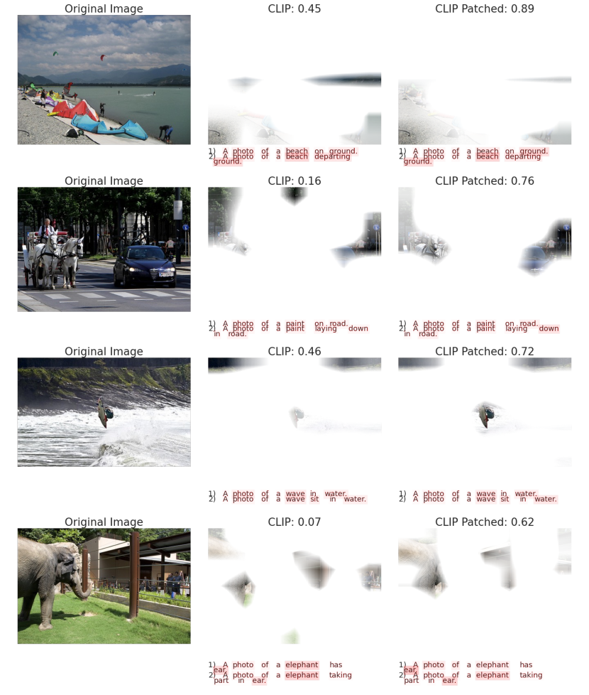
Figure 12: Examples from Probe-R comparing CLIP ViT-B/32 to the same model finetuned on RelComp for both the visual and text encoder, then patched [17]. The values are the softmax confidence for the correct prompt $P_{R_{1}}$ shown as $1)$ vs the incorrect prompt $2)$, where the predicate is swapped, or $P_{R_{2}}$.

Figure 13: Examples from Probe-C comparing CLIP ViT-B/32 to the same model finetuned on RelComp for both the visual and text encoder, then patched [17]. For each group, the first image and its corresponding prompt are on top, and the second image and prompt are on the bottom. The values are the softmax confidence for the corresponding prompt when compared to the alternative prompt.

Figure 14: We design probes that measure relational understanding in V+L models, in this case we compare ViLT [20] that uses cross-attention (top) and CLIP [31] which does not (bottom). With cross-attention, the model can change its focus based on the prompt and performs better when compositions and relations are swapped for unrealistic/non-present ones. Meanwhile, CLIP does not adapt and focuses more highly on objects, like “man” and “skateboard”.

The results for all models for the Probe-R benchmark are shown in Table 4. We include CLIP models we finetuned on RelComp, training either the text encoder (T), visual encoder (V) or both encoders (VT). Training only the text encoder seems to have the highest improvement, but as mentioned in the paper, the largest occurrence of “catastrophic forgetting” when evaluated on ImageNet. A TSNE plot of model features that includes CLIP Patched (VT) is shown in Figure 9. In black we have the image features, in red we have the predicate swapped text features ($P_{R_{2}}$), and in green we have the ground truth relation text features ($P_{R_{1}}$. This finetuned and patched version appears to have tighter clusters compared to the original CLIP model.

A.2 Probe-C: Compositional Understanding

This dataset was generated using MSCOCO [22]. To guarantee that the images had no similarity or overlap, we focused on using antonyms of select attributes. We started by using NLTK POS [3] to find adjective-noun pairs. We then manually cleaned and extracted the adjectives to guarantee the attribute is a visual one such as “red” or “young” as opposed to a subjective one such as “hungry” or “thirsty”. While these are useful attributes, we are primarily interested in visual perception as opposed to subjective inference. We then iterated through all images and mapped each attribute to their corresponding image IDs, and we did the same with objects. Using this collection, we were able to create groups of pairs based on either swapping the attribute to one of its antonyms or swapping the object with one that has the same attribute.

The overall results for Probe-C for all models is in Table 5. The mappings we used to categorize different attributes is shown in Table 6, these were manually generated. A visual break down of different model performances for each attribute is shown in Figure 10. From there, you can see the changes in score based on whether it is matching the caption given the image versus given text. We also see that most models struggle with “visibility” and often “texture”.

A.3 Probe-B: Context Understanding

In set 1, for each image we remove the background using segmentation masks from original annotations. We replace the background with 1 of four fillers: black, gray, Gaussian noise, or a random scene. Random scenery was collected from the Indoor Scenes Dataset [30] and the Kaggle Landscape dataset [34]. These images were manually filtered to ensure none of the 80 MSCOCO classes were present. The total collection is 31,745 images with 4 fillings each for a total of 126,980 images. We filtered images based on a threshold for how much background can be removed to ensure that some context was actually removed. In set 2, for each image we remove all other objects and the background using segmentation masks. In this case, $x_{0}$ is the image with all objects with just the background removed while $\tilde{x_{1}}$ is the image with just one object remaining and all other objects and the background removed. This allows us to isolate whether it is the other objects compared to background removal. Like in set 1, we replace them with the different possible fillers. Images are chosen if they do not have overlapping bounding boxes and if their object area is over a threshold to allow for better visibility. Prompts for set 2 only include objects not present in the original image and the target object.

To better compare CLIP backbones, Figure 11 shows a comparison between the change in confidence from a patched image $\tilde{x_{0}}$ to the image where all other objects and background $\tilde{x_{1}}$ is removed aggregated over CLIP backbones. Table 8 shows what objects are assigned to which category and how many samples are present in the annotations. The main differences are in objects they struggle with by how much and in which order.

Overall results for Probe-B are in Table 9 and 10. In both cases, replacing with scene and noise produces worse results compared to black and gray fillers. For aggregating across filler, we only include CLIP ViT-L/14@336px, CLIP RN50x4, FLAVA, ViLT, and BridgeTower. When comparing individual model results in Table 10, performance tends to increase when only the other object remains, meaning that other objects may actually distract models. BridgeTower is the highest performer and has the lowest robustness from $x_{0}$ to $x_{1}$ meaning that it may be using some level of object relationship understandings to help recognize objects. However, this difference is minor and therefore inconclusive. Other models’ robustness though is higher indicating they perform better when objects are in isolation, indicating they are not using object relationship understanding to help object detection of particular objects. In Table 9, when only background is removed, we see little change. However, in ViLT, which is one transformer that takes both text and visual tokens, adding a patch reduced performance noticeably worse when compared to other models. This may indicate a weakness in a single-stream, transformer based approach.

Appendix B Exploring Improving Dual-Stream Only Conceptual Models

Based on our evaluation of these models, we see that cross-attention between modalities improves the learning of conceptual models about objects and actions in a system and the relationships between them. However, a limitation of this approach is its use for downstream tasks. Both ViLT and BridgeTower require image-text pairs of input, making other tasks like image classification computationally expensive and difficult. Meanwhile, dual-stream encoders like CLIP and FLAVA allow uni-modal feature representations that can be extracted and used for a variety of downstream tasks. Improving models that do not require paired input would provide greater value and stronger representations. To explore this idea, we fine-tune CLIP on a new dataset inspired by this benchmark called RelComp.

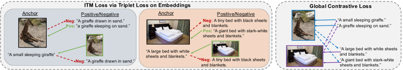
Figure 15: An overview of the training paradigm we propose for improving CLIP’s compositional and relational understanding. Image-text matching (ITM) is used as a triplet loss between an anchor, positive and negative which vary depending on if it is a compositional task or a relational task. A contrastive loss is used to maintain general representations.

B.1 Method

In order to improve CLIP for compositional and relational understanding, we propose using selective negative and positive pairing based on compositional and predicate swaps. We propose using two losses, an image-text matching (ITM) loss and a contrastive loss (C) similar to CLIP [31] and FLAVA [39]. The ITM loss is a triplet loss with two instances [7], maximizing the distance between an anchor and a negative sample while minimizing the distance between an anchor and a positive sample. We use this in order to focus model learning on compositions and relations. The first is where the anchor is the image $x$, the positive is the caption $p$, and the negative $\overline{p}$ is the same caption but with either the predicate or the composition swapped. The second uses a real-world caption $y$ as an anchor and the corresponding image $x$ as a positive. The final ITM loss is the average of the two. For the contrastive loss, we maximize the cosine similarities between image and text pairs and minimize those for the image and negative text pairs. We use two versions, the first uses the real-world captions $y$ and their corresponding images, and the second uses the positive text prompts $p$ and their images. The final contrastive loss is the average of the two. A summary of this approach is shown in Figure 15.

B.2 Dataset: RelComp

We used our existing knowledge of the benchmark to generate a new training and testing dataset. For compositions, we use images and captions from the MSCOCO dataset [22]. For anchor text we use the real-world caption, for positive we replace all compositions with synonyms, and for negatives we replace all compositions with antonyms. No captions seen in this dataset are also seen in Probe-C. For relations, we use images, region descriptions and relationships from the VisualGenome dataset [21]. For each image, we find the region description that has the most overlap with prompts generated in the same way as Probe-R and use this as our anchor caption. For negative, we use the same template but use prompt with the predicate swapped to an unlikely one, as in Probe-R. To prevent exact prompts from the benchmark being included, we filtered for images that are not present in Probe-R. This results in 149,166 groups with 78,155 of those swapping compositions and 71,011 swapping predicates for training. The test set has 15,836 groups and of those, 8,734 are swap compositions and 7,102 swap predicates.

B.3 Implementation

We finetune the CLIP ViT-B/32 model using our proposed ITM and contrastive loss on the proposed dataset RelComp. We use stochastic gradient descent with a cosine learning rate scheduler with a minumum learning rate of .001, momentum 0.9, weight decay of .0001. We train for 40 epochs using an 11GB GPU and a batch size of 128. We use these smaller configurations to show the benefits with just light tuning. One of the many challenges of fine-tuning a large model, is that the distribution shift may lead to a loss of the original feature space. In order to prevent this “catastrophic forgetting” of the original feature space, we linearly interpolate the original CLIP weights with our finetuned weights using an alpha$=0.2$, leaning more towards the original weights, in order to reduce this shift [17, 46]. This is referred to as patching and therefore we call the finetuned and patched version “CLIP Patched”. We finetune three configurations based on which encoders we finetune: visual only (V), text only (T) or both (VT).

B.4 Results

Model	ImageNet	RelComp	Probe-C	Probe-R
ViLT	–	76.00	90.78	69.00
BridgeTower	–	85.00	90.06	82.20
FLAVA	56.83	47.12	83.85	68.29
CLIP ViT B32	63.60	51.93	88.15	53.52
CLIP Patched (T)	57.85	67.85	89.49	71.14
CLIP Patched (V)	61.45	54.66	89.81	61.40
CLIP Patched (VT)	54.61	64.27	90.30	71.20

Figure 16: Overall results for finetuning and patching the CLIP ViT-B/32 on the proposed RelComp dataset. ImageNet accuracy is shown to measure the drift from the original CLIP space. RelComp is the image score for the correct image-to-prompt matching. Probe-C/R are the mean accuracy for the correct image-prompt match. Top scores are in bold while second are underlined.

Overall results for our experiment are shown in Table 3. When finetuning on the new dataset, there is an issue of drift from the original CLIP performance as measured by ImageNet accuracy, even when patching. When finetuning using the visual-encoder only, the drift is less pronounced, but so is the improvement on RelComp. The largest increase in RelComp is seen when just training the text encoder. (1) This may indicate that for non-cross-attention models text is more important for conceptual mapping. Overall, (2) our findings indicate that it is possible by using selective negative sampling to enforce compositional and relational learning without extensive co-attention and computational complexity. Limitations of this experiment is our training data is very small in comparison to recent works, further work should investigate this relationship with a larger dataset with more variation.

Table 11 shows the results based on different alphas for RelComp and ImageNet. There is a definite trade-off between original performance and performance on the new task. We also see that training only the text encoder yields the greatest improvement in these tasks but also the largest “forgetting”. Some examples of where CLIP patched improved over CLIP in Probe-R is shown in Figure 12. The first column are the original images, the second the attention maps of visual and text features for CLIP ViT-B/32 and the third are the attention maps for CLIP Patched (VT). The values are the softmax confidence for the correct prompt $P_{R_{1}}$ shown as $1)$ versus the incorrect prompt $P_{R_{2}}$ where the predicate is switched $2)$. Similar examples for Probe-C are shown in Figure 13. For each group, the first image and its corresponding prompt are on top, and the second image and prompt are on the bottom. The values are the softmax confidence for the corresponding prompt when compared to the alternative prompt.

Appendix C Licensing

In our work we alter the COCO [22] and Visual Genome [21] dataset under the Creative Commons Attribution 4.0 License.This extends to our dataset as they are modifications to these original datasets. BridgeTower [47], FLAVA [39], CLIP [31] and ViLT [20] uses an MIT License. The patching scheme [17] for our exploratory baseline experiment also uses an MIT license. Additionally, code used to implement these models utilizes HuggingFace [45] which has a Pylar AI creative ML License 0.0 license.

Appendix D Model Details

A summary of the model details can be found in Table 12. The highest performing model is BridgeTower but it also had the largest number of parameters and the slowest. Additionally, BridgeTower utilizes a pre-trained CLIP visual encoder, improving upon CLIPs performance. ViLT, BridgeTower and FLAVA all require image-text pairs, making a greater number of comparisons difficult, especially for downstream tasks like image classification on ImageNet where there are 1000 classes. However, because FLAVA merges dual-stream encoder output prior to cross-encoding, it is easier to extract feature embeddings prior to the cross-encoding for a greater number of comparisons. This however does not utilize its full potential for performance. Figure 14 shows examples of how this image-text pair input is a strength for performance in these kinds of tasks. The bottom shows ViLT and how its visual attention changes based on its input while the top shows CLIP which has consistent attention no matter the text, visual input.

Model	MSCOCO				Flicker30
	TR		IR		TR		IR
	R@1	R@5	R@1	R@5	R@1	R@5	R@1	R@5
CLIP ViT-B/16	52.5	76.7	33.0	58.4	82.2	96.6	62.0	85.7
CLIP ViT-L/14@336px	58.4	84.5	37.8	62.4	88.0	98.7	68.7	90.6
FLAVA	42.7	76.8	38.4	67.5	60.9	88.9	56.5	83.6
ViLT	61.5	86.3	42.7	72.9	83.5	96.7	64.4	88.7
BridgeTower	75.0	90.2	62.4	85.1	94.7	99.6	85.8	97.6

Table 13: An overview of image-to-text retrieval (TR) and text-to-image retrieval (IR) results on the MSCOCO [22] and Flicker30 [48] as reported by the authors. CLIP is the only model that is not pre-trained with MSCOCO and has comparable performance.

Table 13 shows the reported results for the selected models and some CLIP models on the MSCOCO [22] and Flicker [48] datasets. We do see correlation between performance on these datasets and performance on the proposed datasets in this benchmark. This indicates that retrieval tasks on datasets like MSCOCO may be a good indicator of “understanding” at a high-level. Code to run these models is

Appendix E Impact

To our understanding, there are no negative societal impacts of our work. The goal of this work was to evaluate the robustness of models that may later be used in real-world settings. We aimed to improve the societal impacts by evaluating these models on real-world distribution shifts including potential bias in text.

Appendix F Limitations

This study has several limitations which include 1) using frequency of co-occurring relationships in annotated datasets can result in pairings that may still be sensible in real-world scenarios. This is mitigated by creating a large dataset such that the noise is not impacting results. 2) Reliance on annotation from the original dataset may leave mistakes in objects or missing objects that should have been annotated. 3) There is much evidence that how a model is prompted can affect performance. Because of computational limitations of these large models, we used “a photo of” consistently through our experiments. However, performance might vary if this template were altered. 4) The analysis is on a limited number of models due to availability of usable code and model weights. The analysis provided is limited to the models we have used in this study. We tried our best to benchmark all publicly available models that provided weights and used both text and video.

Appendix G Dataset Sheet for Dataset

G.1 Motivation

The core motivation for this dataset was to study the underlying understanding of object and their relationships to other objects, attributes, and background information when matching a caption to an image. This could further help moving the field by studying underlying model behavior and where models could be improved.

G.2 Composition

Content and Composition: Probe-R

The instances in this dataset consist of “groups”. Each group consists of one anchor image, ten positive images and ten negative images. Positive images are images with the same object as the anchor image with no other overlapping objects, based on the original COCO annotations. Negative images are images with the swapped object and no other overlapping objects, based on the original COCO annotations. It contains four prompts, the anchor image prompt of “a photo of a $<$subject$>$ $<$predicate$>$ $<$object$>$”, a positive image prompt “a photo of a $<$subject$>$”, a negative predicate prompt “a photo of a $<$subject¿ $<$swapped predicate$>$ $<$object$>$”, and a negative object prompt “a photo of a $<$swapped subject$>$ $<$predicate$>$ $<$object$>$”. There are a total of 99,960 annotated groups. Overall, the dataset consists of 6,006 objects and 2,536 predicates, or relationship aliases.

Content and Composition: Probe-C

The instances in this dataset consists of “groups”. Each group consists of two images and two prompts. There are two set of groups. The first set of groups has one image and prompt and a second image and prompt where the attribute in the image and prompt are the antonym of the first image. There are 79,925 groups in this set. The second set of groups is the same but with the object swapped. There are 385,580 groups. Overall, there are a total of 114 attributes/compositions and 790 objects.

Content and Composition: Probe-B

The instances in this dataset consists of “groups”. There are two sets of groups. The first set of groups contains an image with its background replaced, but all foreground objects in the original COCO annotation remaining, and the original COCO instance annotations. There are 31,765 unique images with four filler types, resulting in 127,060 total images. There are a total of 80 object types. For the second set, there is a single image and one object where the background and all other objects are replaced with a filler. There are a total of 9,375 unique object images from 2,259 unique COCO images, with four fillers, resulting in 37,500 total images. There are a total of 79 objects because there were some noticeable annotation problems with the object “apple”.

Does the dataset contain all possible instances or is it a sample (not necessarily random) of instances from a larger set?

Probe-C and Probe-B are a subset of COCO [22] while Probe-R is a subset of Visual Genome [21].

Are relationships between individual instances made explicit (e.g., users’ movie ratings, social network links)?

No.

Are there recommended data splits (e.g., training, development/validation, testing)?

No, these datasets are used for benchmark evaluation only.

Are there any errors, sources of noise, or redundancies in the dataset?

Any annotation noise from the original COCO [22] and Visual Genome [21] datasets may also be present in this dataset. There may be additional noise from prompt generation in Probe-R where unlikely events may still be possible. We mitigate this by making a large dataset with many samples.

Is the dataset self-contained, or does it link to or otherwise rely on external resources (e.g., websites, tweets, other datasets)?

This dataset is self-contained by our provided download instructions, but its generation relies on the existing datasets COCO [22] and Visual Genome [21].

Is there a label or target associated with each instance?

Yes, each group has a matching prompt(s) to image.

Does the dataset contain data that might be considered sensitive in any way (e.g., data that reveals race or ethnic origins, sexual orientations, religious beliefs, political opinions or union memberships, or locations; financial or health data; biometric or genetic data; forms of government identification, such as social security numbers; criminal history)?

No.

Does the dataset contain data that might be considered sensitive in any way (e.g., data that reveals race or ethnic origins, sexual orientations, religious beliefs, political opinions or union memberships, or locations; financial or health data; biometric or genetic data; forms of government identification, such as social security numbers; criminal history)?

No.

Does the dataset contain data that, if viewed directly, might be offensive, insulting, threatening, or might otherwise cause anxiety?

No.

Does the dataset identify any subpopulations (e.g., by age, gender)?

No.

Is it possible to identify individuals (i.e., one or more natural persons), either directly or indirectly (i.e., in combination with other data) from the dataset?

No, while individuals are visible in images, there is no known way to match the individual to an identity.

G.3 Collection Process

Each instance in the Probe-R, Probe-C, and Probe-B were extracted and modified directly from existing datasets COCO [22] and Visual Genome [21].

What mechanisms or procedures were used to collect the data (e.g., hardware appara tuses or sensors, manual human curation, software programs, software APIs)?

Code and download links were provided by COCO [22] and Visual Genome [21].

If the dataset is a sample from a larger set, what was the sampling strategy (e.g., deterministic, probabilistic with specific sampling probabilities)?

For Probe-R, samples were selected based on if they had a manually refined list of predicates. These were manually cleaned by confirming they were in did describing a relationship/action between two objects. From that selection, we than randomly sampled. For Probe-C, this was similar but for attributes. For example, some attributes were not visible such as “hungry” or “thirsty”. We refined this list based on visible attributes. For Probe-B, we refined based on the object sizes. If when the background is removed and all objects remained, a threshold of image still remains, we discarded the image. If when both the background and the other objects are removed, an object that was below a size threshold or greater than a size threshold was discarded.

Did you collect the data from the individuals in question directly, or obtain it via third parties or other sources (e.g., websites)

Both COCO [22] and Visual Genome [21] are publicaly available for use under the Creative Commons Attribution 4.0 License

G.4 Labelling/Preprocessing/Cleaning

Probe-R

This dataset is built off of Visual Genome [21]. This dataset was created by cleaning the annotations/relationship aliases with relations that are specifically an interaction rather than an attribute which was often an erroneous annotation and grouping relations that are the same despite spelling errors. Objects and predicates are additionally cleaned based on spelling errors. Using the extracted (subject, predicate, object) triplets, unlikely relationships are determined if there is no existing combination of an object-predicate pair or subject-object pair. For each image, the ground truth relation is compared to a highly unlikely swap of subject and predicate. There are set of ”positive” images that are images with the subject being swapped and no other objects from the original image. There are also a set of ”negative” images that are images with the swapped subject and no other objects from the original image. The predicate swapped is based on the predicates that have not been found in the original dataset to be associated with the original subject and therefore are highly unlikely.

Probe-C

This dataset is built of the COCO Validation 2014 [22] dataset. Using the NLP library NLTK [4] and the COCO caption annotations, words are tagged and pairs of adjective and nouns are extracted. These pairs are then manually cleaned to ensure the attribute is indeed an adjective and the object is indeed an object. Instead of using unlikely combinations, antonyms were manually mapped to each attribute in order to ensure that the attribute is not present in the image. For example, if there is a ”a small dog”, the comparison prompt is ”a large dog”. There are two splits for this dataset. The first is where the composition is swapped with an antonym and the other is where an object is switched. Each dataset has two images and two captions and comparisons are based on how well the model can match the captions to the correct images.

Probe-B

This dataset is built off COCO Validation 2014 [22] dataset. Segmentation annotations from the original COCO dataset were used for removing background and/or objects. For set 1, for each image, it removes all other objects using either the segmentation(retaining shape cues). These are replaced with either “black”, “gray”, “scene” or ”noise”. Images are chosen if they do not have overlapping bounding boxes and if their object area is over a threshold to allow for better visibility, making the task easier. “Scene” fillers are extracted from landscape scenery from a subset of the Kaggle Landscape dataset [33] and Indoor Scenes Dataset [30]. The subset of 290 scene filler images were selected based on whether there were any objects in the image that are also in the annotations.

G.5 Uses

Has the dataset been used for any tasks already?

For benchmarking performance on visual-language models for image-text matching.

Is there a repository that links to any or all papers or systems that use the dataset?

The benchmark along with the code and datasets is available at: https://tinyurl.com/vlm-robustness

What (other) tasks could the dataset be used for?

Compositional learning, robust scene graph, and robust object recognition/detection.

Is there anything about the composition of the dataset or the way it was collected and preprocessed/cleaned/labeled that might impact future uses

Not that we are aware of.

Are there tasks for which the dataset should not be used?

No.

G.6 Distribution

Will the dataset be distributed to third parties outside the entity (e.g., company, institution, organization) on behalf of which the dataset was created?

No.

How will the dataset be distributed (e.g., tarball on website, API, GitHub)?

Available at: https://tinyurl.com/vlm-robustness

When will the dataset be distributed?

It is currently available for download.

Will the dataset be distributed under a copyright or other intellectual property (IP) license, and/or under applicable terms of use (ToU)?

Datasets will be distributed under Creative Commons License.

Have any third parties imposed IP-based or other restrictions on the data associated with the instances?

No.

Do any export controls or other regulatory restrictions apply to the dataset or to individual instances?

No.

References

- [1] Jean-Baptiste Alayrac, Jeff Donahue, Pauline Luc, Antoine Miech, Iain Barr, Yana Hasson, Karel Lenc, Arthur Mensch, Katie Millican, Malcolm Reynolds, et al. Flamingo: a visual language model for few-shot learning. arXiv preprint arXiv:2204.14198, 2022.
- [2] Renee Baillargeon. Object permanence in 3-and 4-month-old infants. Developmental psychology, 23(5):655, 1987.
- [3] Steven Bird, Ewan Klein, and Edward Loper. Natural language processing with Python: analyzing text with the natural language toolkit. ” O’Reilly Media, Inc.”, 2009.
- [4] Steven Bird, Ewan Klein, and Edward Loper. Natural language processing with Python: analyzing text with the natural language toolkit. ” O’Reilly Media, Inc.”, 2009.
- [5] Nicholas Carlini, Jamie Hayes, Milad Nasr, Matthew Jagielski, Vikash Sehwag, Florian Tramèr, Borja Balle, Daphne Ippolito, and Eric Wallace. Extracting training data from diffusion models. arXiv preprint arXiv:2301.13188, 2023.
- [6] Soravit Changpinyo, Piyush Sharma, Nan Ding, and Radu Soricut. Conceptual 12m: Pushing web-scale image-text pre-training to recognize long-tail visual concepts. In Proceedings of the IEEE/CVF Conference on Computer Vision and Pattern Recognition, pages 3558–3568, 2021.
- [7] Gal Chechik, Varun Sharma, Uri Shalit, and Samy Bengio. Large scale online learning of image similarity through ranking. Journal of Machine Learning Research, 11(3), 2010.
- [8] for Social Security Administration Disability Determinations; Board on the Health of Select Populations; Institute of Medicine Committee on Psychological Testing, Including Validity Testing. Psychological testing in the service of disability determination, 2015.
- [9] Jia Deng, Wei Dong, Richard Socher, Li-Jia Li, Kai Li, and Li Fei-Fei. Imagenet: A large-scale hierarchical image database. In 2009 IEEE conference on computer vision and pattern recognition, pages 248–255. Ieee, 2009.
- [10] Karan Desai, Gaurav Kaul, Zubin Aysola, and Justin Johnson. Redcaps: Web-curated image-text data created by the people, for the people. arXiv preprint arXiv:2111.11431, 2021.
- [11] Anuj Diwan, Layne Berry, Eunsol Choi, David Harwath, and Kyle Mahowald. Why is winoground hard? investigating failures in visuolinguistic compositionality. arXiv preprint arXiv:2211.00768, 2022.
- [12] Alexey Dosovitskiy, Lucas Beyer, Alexander Kolesnikov, Dirk Weissenborn, Xiaohua Zhai, Thomas Unterthiner, Mostafa Dehghani, Matthias Minderer, Georg Heigold, Sylvain Gelly, Jakob Uszkoreit, and Neil Houlsby. An image is worth 16x16 words: Transformers for image recognition at scale. ICLR, 2021.
- [13] Sivan Doveh, Assaf Arbelle, Sivan Harary, Amit Alfassy, Roei Herzig, Donghyun Kim, Raja Giryes, Rogerio Feris, Rameswar Panda, Shimon Ullman, et al. Dense and aligned captions (dac) promote compositional reasoning in vl models. arXiv preprint arXiv:2305.19595, 2023.
- [14] Sivan Doveh, Assaf Arbelle, Sivan Harary, Eli Schwartz, Roei Herzig, Raja Giryes, Rogerio Feris, Rameswar Panda, Shimon Ullman, and Leonid Karlinsky. Teaching structured vision & language concepts to vision & language models. In Proceedings of the IEEE/CVF Conference on Computer Vision and Pattern Recognition, pages 2657–2668, 2023.
- [15] Steven M. Frankland and Joshua D. Greene. Concepts and compositionality: In search of the brain’s language of thought. Annual Review of Psychology, 71(1):273–303, 2020.
- [16] Robert Geirhos, Patricia Rubisch, Claudio Michaelis, Matthias Bethge, Felix A Wichmann, and Wieland Brendel. Imagenet-trained cnns are biased towards texture; increasing shape bias improves accuracy and robustness. arXiv preprint arXiv:1811.12231, 2018.
- [17] Gabriel Ilharco, Mitchell Wortsman, Samir Yitzhak Gadre, Shuran Song, Hannaneh Hajishirzi, Simon Kornblith, Ali Farhadi, and Ludwig Schmidt. Patching open-vocabulary models by interpolating weights. NeurIPs, 2022.
- [18] Justin Johnson, Bharath Hariharan, Laurens van der Maaten, Li Fei-Fei, C. Lawrence Zitnick, and Ross Girshick. Clevr: A diagnostic dataset for compositional language and elementary visual reasoning. In Proceedings of the IEEE Conference on Computer Vision and Pattern Recognition (CVPR), July 2017.
- [19] Amita Kamath, Jack Hessel, and Kai-Wei Chang. Text encoders are performance bottlenecks in contrastive vision-language models. arXiv preprint arXiv:2305.14897, 2023.
- [20] Wonjae Kim, Bokyung Son, and Ildoo Kim. Vilt: Vision-and-language transformer without convolution or region supervision. In International Conference on Machine Learning, pages 5583–5594. PMLR, 2021.
- [21] Ranjay Krishna, Yuke Zhu, Oliver Groth, Justin Johnson, Kenji Hata, Joshua Kravitz, Stephanie Chen, Yannis Kalanditis, Li-Jia Li, David A Shamma, Michael Bernstein, and Li Fei-Fei. Visual genome: Connecting language and vision using crowdsourced dense image annotations. 2016.
- [22] Tsung-Yi Lin, Michael Maire, Serge Belongie, James Hays, Pietro Perona, Deva Ramanan, Piotr Dollár, and C Lawrence Zitnick. Microsoft coco: Common objects in context. In Computer Vision–ECCV 2014: 13th European Conference, Zurich, Switzerland, September 6-12, 2014, Proceedings, Part V 13, pages 740–755. Springer, 2014.
- [23] Yinhan Liu, Myle Ott, Naman Goyal, Jingfei Du, Mandar Joshi, Danqi Chen, Omer Levy, Mike Lewis, Luke Zettlemoyer, and Veselin Stoyanov. Roberta: A robustly optimized bert pretraining approach. arXiv preprint arXiv:1907.11692, 2019.
- [24] Zixian Ma, Jerry Hong, Mustafa Omer Gul, Mona Gandhi, Irena Gao, and Ranjay Krishna. Crepe: Can vision-language foundation models reason compositionally? In Proceedings of the IEEE/CVF Conference on Computer Vision and Pattern Recognition, pages 10910–10921, 2023.
- [25] Richard E Mayer. Models for understanding. Review of educational research, 59(1):43–64, 1989.
- [26] Mazda Moayeri, Phillip Pope, Yogesh Balaji, and Soheil Feizi. A comprehensive study of image classification model sensitivity to foregrounds, backgrounds, and visual attributes. In Proceedings of the IEEE/CVF Conference on Computer Vision and Pattern Recognition, pages 19087–19097, 2022.
- [27] Letitia Parcalabescu, Michele Cafagna, Lilitta Muradjan, Anette Frank, Iacer Calixto, and Albert Gatt. VALSE: A task-independent benchmark for vision and language models centered on linguistic phenomena. In Proceedings of the 60th Annual Meeting of the Association for Computational Linguistics (Volume 1: Long Papers), pages 8253–8280, Dublin, Ireland, May 2022. Association for Computational Linguistics.
- [28] Genevieve Patterson and James Hays. Coco attributes: Attributes for people, animals, and objects. In Computer Vision–ECCV 2016: 14th European Conference, Amsterdam, The Netherlands, October 11-14, 2016, Proceedings, Part VI 14, pages 85–100. Springer, 2016.
- [29] Luis S Piloto, Ari Weinstein, Peter Battaglia, and Matthew Botvinick. Intuitive physics learning in a deep-learning model inspired by developmental psychology. Nature human behaviour, 6(9):1257–1267, 2022.
- [30] Ariadna Quattoni and Antonio Torralba. Recognizing indoor scenes. In 2009 IEEE conference on computer vision and pattern recognition, pages 413–420. IEEE, 2009.
- [31] Alec Radford, Jong Wook Kim, Chris Hallacy, Aditya Ramesh, Gabriel Goh, Sandhini Agarwal, Girish Sastry, Amanda Askell, Pamela Mishkin, Jack Clark, et al. Learning transferable visual models from natural language supervision. In International conference on machine learning, pages 8748–8763. PMLR, 2021.
- [32] Yongming Rao, Wenliang Zhao, Guangyi Chen, Yansong Tang, Zheng Zhu, Guan Huang, Jie Zhou, and Jiwen Lu. Denseclip: Language-guided dense prediction with context-aware prompting. In Proceedings of the IEEE/CVF Conference on Computer Vision and Pattern Recognition (CVPR), pages 18082–18091, June 2022.
- [33] Arnaud ROUGETET. Kaggle landscape dataset. https://www.kaggle.com/datasets/arnaud58/landscape-pictures/.
- [34] Arnaud Rougetet. Landscape pictures. https://www.kaggle.com/datasets/arnaud58/landscape-pictures, 2021. Accessed: February 16, 2023.
- [35] Pritish Sahu, Michael Cogswell, Yunye Gong, and Ajay Divakaran. Unpacking large language models with conceptual consistency. arXiv preprint arXiv:2209.15093, 2022.
- [36] Christoph Schuhmann, Richard Vencu, Romain Beaumont, Robert Kaczmarczyk, Clayton Mullis, Aarush Katta, Theo Coombes, Jenia Jitsev, and Aran Komatsuzaki. Laion-400m: Open dataset of clip-filtered 400 million image-text pairs. arXiv preprint arXiv:2111.02114, 2021.
- [37] Piyush Sharma, Nan Ding, Sebastian Goodman, and Radu Soricut. Conceptual captions: A cleaned, hypernymed, image alt-text dataset for automatic image captioning. In Proceedings of the 56th Annual Meeting of the Association for Computational Linguistics (Volume 1: Long Papers), pages 2556–2565, Melbourne, Australia, July 2018. Association for Computational Linguistics.
- [38] Piyush Sharma, Nan Ding, Sebastian Goodman, and Radu Soricut. Conceptual captions: A cleaned, hypernymed, image alt-text dataset for automatic image captioning. In Proceedings of the 56th Annual Meeting of the Association for Computational Linguistics (Volume 1: Long Papers), pages 2556–2565, Melbourne, Australia, July 2018. Association for Computational Linguistics.
- [39] Amanpreet Singh, Ronghang Hu, Vedanuj Goswami, Guillaume Couairon, Wojciech Galuba, Marcus Rohrbach, and Douwe Kiela. Flava: A foundational language and vision alignment model. In Proceedings of the IEEE/CVF Conference on Computer Vision and Pattern Recognition, pages 15638–15650, 2022.
- [40] Robyn Speer, Joshua Chin, and Catherine Havasi. Conceptnet 5.5: An open multilingual graph of general knowledge. In Proceedings of the AAAI conference on artificial intelligence, volume 31, 2017.
- [41] Krishna Srinivasan, Karthik Raman, Jiecao Chen, Michael Bendersky, and Marc Najork. Wit: Wikipedia-based image text dataset for multimodal multilingual machine learning. In Proceedings of the 44th International ACM SIGIR Conference on Research and Development in Information Retrieval, pages 2443–2449, 2021.
- [42] Bart Thomee, David A. Shamma, Gerald Friedland, Benjamin Elizalde, Karl Ni, Douglas Poland, Damian Borth, and Li-Jia Li. Yfcc100m: The new data in multimedia research. Commun. ACM, 59(2):64–73, jan 2016.
- [43] Tristan Thrush, Ryan Jiang, Max Bartolo, Amanpreet Singh, Adina Williams, Douwe Kiela, and Candace Ross. Winoground: Probing vision and language models for visio-linguistic compositionality. In Proceedings of the IEEE/CVF Conference on Computer Vision and Pattern Recognition, pages 5238–5248, 2022.
- [44] Zhaoqing Wang, Yu Lu, Qiang Li, Xunqiang Tao, Yandong Guo, Mingming Gong, and Tongliang Liu. Cris: Clip-driven referring image segmentation. In Proceedings of the IEEE/CVF Conference on Computer Vision and Pattern Recognition (CVPR), pages 11686–11695, June 2022.
- [45] Thomas Wolf, Lysandre Debut, Victor Sanh, Julien Chaumond, Clement Delangue, Anthony Moi, Pierric Cistac, Tim Rault, Rémi Louf, Morgan Funtowicz, et al. Transformers: State-of-the-art natural language processing. In Proceedings of the 2020 conference on empirical methods in natural language processing: system demonstrations, pages 38–45, 2020.
- [46] Mitchell Wortsman, Gabriel Ilharco, Jong Wook Kim, Mike Li, Simon Kornblith, Rebecca Roelofs, Raphael Gontijo Lopes, Hannaneh Hajishirzi, Ali Farhadi, Hongseok Namkoong, et al. Robust fine-tuning of zero-shot models. In Proceedings of the IEEE/CVF Conference on Computer Vision and Pattern Recognition, pages 7959–7971, 2022.
- [47] Xiao Xu, Chenfei Wu, Shachar Rosenman, Vasudev Lal, and Nan Duan. Bridge-tower: Building bridges between encoders in vision-language representation learning. arXiv preprint arXiv:2206.08657, 2022.
- [48] Peter Young, Alice Lai, Micah Hodosh, and Julia Hockenmaier. From image descriptions to visual denotations: New similarity metrics for semantic inference over event descriptions. Transactions of the Association for Computational Linguistics, 2:67–78, 2014.
- [49] Mert Yuksekgonul, Federico Bianchi, Pratyusha Kalluri, Dan Jurafsky, and James Zou. When and why vision-language models behave like bag-of-words models, and what to do about it? arXiv preprint arXiv:2210.01936, 2022.
- [50] Mert Yuksekgonul, Federico Bianchi, Pratyusha Kalluri, Dan Jurafsky, and James Zou. When and why vision-language models behave like bags-of-words, and what to do about it? In The Eleventh International Conference on Learning Representations, 2022.
- [51] Tiancheng Zhao, Tianqi Zhang, Mingwei Zhu, Haozhan Shen, Kyusong Lee, Xiaopeng Lu, and Jianwei Yin. Vl-checklist: Evaluating pre-trained vision-language models with objects, attributes and relations. arXiv preprint arXiv:2207.00221, 2022.
- [52] Kaiyang Zhou, Jingkang Yang, Chen Change Loy, and Ziwei Liu. Conditional prompt learning for vision-language models. In Proceedings of the IEEE/CVF Conference on Computer Vision and Pattern Recognition, pages 16816–16825, 2022.