Graphon Estimation in bipartite graphs with observable edge labels and unobservable node labels

Abstract

Many real-world data sets can be presented in the form of a matrix whose entries correspond to the interaction between two entities of different natures (the choice of a product by a customer, the number of times a web user visits a web page, a student’s grade in a subject, a patient’s rating of a doctor, etc.). We assume in this paper that the mentioned interaction is determined by unobservable latent variables describing each entity. Our objective is to estimate the conditional expectation of the data matrix given the unobservable variables. This is presented as a problem of estimation of a bivariate function referred to as graphon. We study the cases of piecewise constant and Hölder-continuous graphons. We establish finite sample risk bounds for the least squares estimator and the exponentially weighted aggregate. These bounds highlight the dependence of the estimation error on the size of the data set, the maximum intensity of the interactions, and the level of noise. As the analyzed least-squares estimator is intractable, we propose an adaptation of Lloyd’s alternating minimization algorithm to compute an approximation of the least-squares estimator. Finally, we present numerical experiments in order to illustrate the empirical performance of the graphon estimator on synthetic data sets.

, , , and

1 Introduction

In this paper, we consider the problem of estimating the conditional mean of a random matrix generated by a bivariate graphon and (unobserved) latent variables. More precisely, let $n$ and $m$ be two positive integers assumed to be large, and $\mathbf{H}$ be an $n\times m$ random matrix with real entries $H_{i,j}$. We assume that the distribution of this matrix $\mathbf{H}$ satisfies the following condition.

Assumption 1.

There is a function $W^{*}:[0,1]^{2}\to\mathbb{R}$, called the graphon, and two random vectors $\boldsymbol{U}=(U_{1},\ldots,U_{n})$ and $\boldsymbol{V}=(V_{1},\ldots,V_{m})$ such that

• the random variables $U_{1},\ldots,U_{n},V_{1},\ldots,V_{m}$ are independent and drawn from the uniform distribution $\mathcal{U}([0,1])$.

• conditionally to $(\boldsymbol{U},\boldsymbol{V})$, the entries $H_{i,j}$ are independent and $\mathbb{E}[H_{i,j}|\boldsymbol{U},\boldsymbol{V}]=W^{*}(U_{i},V_{j})$.

The aforementioned setting corresponds to the practical situation in which there are $n$ customers and $m$ products. Each customer has an unobserved latent feature $U$ and each product has an unobserved latent feature $V$. We observe the label $H$ that characterizes the interaction between the customer and the product (typically, that the customer chose the product). The function $W^{*}$ corresponds to the mean value of the interaction for given values of the latent features.

The scope of applicability for both the aforementioned framework and the results derived in this paper encompasses the following main examples:

1. The entries $H_{i,j}$ take the values $0$ or $1$ and correspond to the presence of an edge in the bipartite graph. In the example of customers and products, one might set $H_{i,j}=1$ if and only if customer $i$ has already bought the product $j$. It is important in this setting to take into consideration the case of large and sparse graphs, in which the probabilities of having an edge between two nodes are small for all pairs of nodes.

2. The provided data is composed of an aggregation of $N$ instances of the customer-product graph outlined in the preceding paragraph. Each entry $H_{i,j}$ signifies the observed frequency of customer $i$ purchasing product $j$. For instance, in a scenario where the customer visited the store $N=10$ times and $H_{i,j}=3/10$, it indicates that the customer acquired product $i$ on three out of ten occasions. In this context, the range of values for $H_{i,j}$ spans from 0 to 1. Assuming independence across the aforementioned $N$ trials, the variance of $H_{i,j}$ scales with the order of $1/N$. As a result, this framework exhibits the distinctive trait of having low-noise variance. This particular instance can be encompassed within a broader context of a sub-Gaussian distribution characterized by a small variance parameter $\sigma^{2}$, which corresponds to $1/N$.

3. The provided data corresponds to observations collected within a time window of duration $T>0$. Each $H_{i,j}$ represents the average occurrences of customer $i$ purchasing product $j$ over the time interval with a length of $T>0$. This scenario can be expressed using the formula $H_{i,j}=N_{i,j}(T)/T$, where $N_{i,j}(T)$ denotes a Poisson random variable characterized by an intensity proportional to $T$. The parameter $T$ may be large, thereby facilitating accurate estimation. It is important to distinguish this example from the prior one in which the values of $H_{i,j}$ were confined to the interval $[0,1]$. In the current context, the values of $H_{i,j}$ are not subject to such constraints and can vary arbitrarily in magnitude.

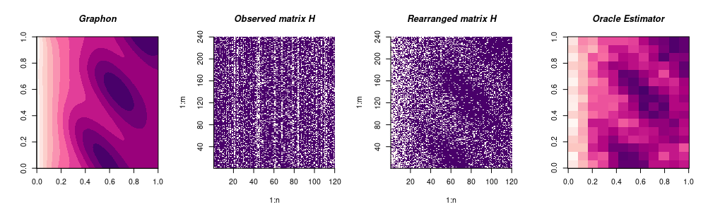
Figure 1: An illustration of the graphon problem. The leftmost graph represents the unknown graphon $W^{*}$. The second leftmost graph is the adjacency matrix observed in the graph where the links are made according to the Bernoulli model. The third graph is the adjacency matrix that would be obtained after a rearrangement of the rows and columns if we had access to the latent variables. The rightmost graph represents the histogram estimator obtained from the rearranged adjacency matrix. Our goal is to design an estimator which is nearly as good as the oracle, without having access to the latent variables.

Our goal is to study the minimax risk of estimating $W^{*}$ and to highlight its dependence on the important parameters of the problem. The sizes $n$ and $m$ of the matrix are among these parameters, but we will also be interested in the dependence on the smoothness of $W^{*}$, on the “sparsity” of interactions (denoted by $\rho$) and on the noise level (denoted by $\sigma$). These parameters $\rho$ and $\sigma$ are positive real numbers such that

$$\|W^{*}\|_{\infty}=\sup_{u,v\in[0,1]}|W^{*}(u,v)|\leqslant\rho\quad\text{and}\quad\mathbf{Var}[H_{i,j}|U_{i},V_{j}]\leqslant\sigma^{2}\ \text{a.s.},\quad\forall i\in[n],\forall j\in[m].$$ (1)

The parameters $\rho$ and $\sigma$ may depend on $n$ and $m$, but we choose to write $\rho$ instead of $\rho_{n,m}$ and $\sigma_{n,m}$ for the sake of simplicity.

During the process of estimating the graphon $W^{*}$, an important intermediate step involves the estimation of the matrix $\boldsymbol{\Theta}^{*}=W^{*}(U_{i},V_{j})$. This matrix estimation holds significant value in its own right. We perform this task by solving the least squares problem over the set of constant-by-block matrices, with blocks generated by partitions of the sets of rows and the columns of the matrix $\mathbf{H}$. It will be further shown that the method of aggregation by exponential weights can be used to ensure adaptivity to the number of blocks. Under the condition that the graphon is piecewise constant or $\alpha$-smooth in the sense of Hölder smoothness, we establish risk bounds for the graphon estimator derived from the estimator of $\boldsymbol{\Theta}^{*}$. These risk bounds are nonasymptotic, and shown to be rate optimal in the minimax sense for a broad range of regimes.

1.1 Measuring the quality of an estimator

Figure 1 provides an illustration of the graphon estimation problem, in the case where $\mathbf{H}$ is the adjacency matrix of the bipartite graph, that is the entries of $\mathbf{H}$ are either 0 or 1. We see in this figure that the absence of knowledge of the latent variables has a strong impact on the recovery of the graphon. Indeed, the adjacency matrix $\mathbf{H}$ depicted in the second leftmost plot carries little information on $W^{*}$, as compared with the rearranged adjacency matrix displayed in the third plot. In fact, when $\boldsymbol{U}$ and $\boldsymbol{V}$ are unknown the graphon $W^{*}$ is unidentifiable. Let us say that two graphons $W$ and $W^{\prime}$ are equivalent, if there exist two bijections that preserve the Lebesgue measure $\tau_{1}:[0,1]\to[0,1]$ and $\tau_{2}:[0,1]\to[0,1]$ such that $W=W^{\prime}\circ(\tau_{1}\otimes\tau_{2})$. One can check that two matrices $\mathbf{H}$ generated by equivalent graphons $W^{*}$ and $\bar{W}^{*}$ have the same distribution. This implies that one can at best estimate the equivalence class containing $W^{*}$. This is the reason underlying the (pseudo)-distance we use in this work for measuring the quality of an estimator $\widehat{W}$ of $W^{*}$, namely

$$\delta(\widehat{W},W^{*}) =\inf_{\tau_{1},\tau_{2}\in\mathcal{M}}\bigg{(}\iint_{[0,1]^{2}}\big{|}\widehat{W}(\tau_{1}(u),\tau_{2}(v))-W^{*}(u,v)\big{|}^{2}du\,dv\bigg{)}^{\nicefrac{{1}}{{2}}}$$ (2)

$$=\inf_{\tau_{1},\tau_{2}\in\mathcal{M}}\|\widehat{W}\circ(\tau_{1}\otimes\tau_{2})-W^{*}\|_{\mathbb{L}^{2}}$$ (3)

where $\mathcal{M}$ is the set of all automorphisms $\tau:[0,1]\to[0,1]$ such that $\tau$ and $\tau^{-1}$ are measurable, and $\tau$ preserves the Lebesgue measure in the sense that $\lambda(\tau^{-1}(B))=\lambda(B)$ for every Borel-set $B\subset[0,1]$. Two graphons $W_{1}$ and $W_{2}$ are called weakly isomorphic if $\delta(W_{1},W_{2})=0$.

1.2 Our contributions

The main contributions of the present paper are the following:

• We present a nonparametric framework based on bivariate graphon functions and unobservable latent variables that offer a flexible way of modeling random matrices and, in particular, adjacency matrices of random bipartite graphs.

• We establish finite sample risk bounds for the estimator minimizing the squared error over piecewise constant matrices with a given number of clusters, as well as for the exponentially weighted aggregate that combines the mentioned least-squares estimators. These results apply to adjacency matrices of bipartite graphs, whose entries are drawn from the Bernoulli distribution, but they are also valid for the binomial distribution, the scaled Poisson distribution and sub-Gaussian distributions.

• We present an adaptation of Lloyd’s algorithm of alternating minimization (including a step of convex relaxation) to our setting, which allows us to obtain a computationally tractable approximation of the least squares estimator.

• In the case of matrices with entries whose conditional distribution given latent variables is the Bernoulli one, we prove lower bounds on the worst-case risk, over the set of piecewise constant graphons, for any graphon estimator. These lower bounds, in the vast majority of cases, are of the same order as the upper bounds obtained for the least-squares estimator.

1.3 Prior work

Statistical analysis of matrix and network data, based on block models similar to those considered in this work, is an active area of research since at least two decades. The stochastic block model, introduced by Holland et al. (1983), is perhaps one of the most studied latent structures for network data, see also (Nowicki and Snijders, 2001) and (Govaert and Nadif, 2003) for early references. Community detection, which is the problem of detecting the underlying block structure, has been the focus of much research effort, as evidenced by studies such as (Zhao et al., 2012; Chin et al., 2015; Lei and Rinaldo, 2015; Lei, 2016; Zhang and Zhou, 2016; Wang and Bickel, 2017; Chen et al., 2018; Xu et al., 2020) and literature reviews such as (Gao et al., 2017; Abbe, 2018). It should be noted that the majority of these studies focused on unipartite graphs with binary or discrete edge-labels, and their optimality was mostly related to identifying the smallest separation rate between the parameters of the communities that enables their consistent recovery. Similar problems for bipartite block models have been investigated in (Feldman et al., 2015; Florescu and Perkins, 2016; Neumann, 2018; Zhou and Amini, 2019a, 2020; Cai et al., 2021; Ndaoud et al., 2022).

In contrast with the aforementioned papers, the focus here is on optimality in terms of the estimation error for a model that encompasses bipartite graphs with real-valued edge labels. Consistency of graphon estimators has been studied in (Airoldi et al., 2013; Wolfe and Olhede, 2013; Olhede and Wolfe, 2014). In the same problem, minimax-rate-optimality of the least squares estimator has been established in (Gao et al., 2015, 2016; Klopp et al., 2017; Klopp and Verzelen, 2019), see also the survey article (Gao and Ma, 2021). To better present our contributions within the current state-of-the-art, it would be beneficial to provide a brief overview of the contents of these papers. Gao et al. (2015) considered the case of binary observations $H_{i,j}$, focusing on the dense case $\rho\asymp 1$, and obtained minimax rates of estimation over the classes of piecewise constant and Hölder continuous graphons. Gao et al. (2016) extended these results to matrices $\mathbf{H}$ with sub-Gaussian entries, some of which might be missing completely at random. However, as discussed in Section 3.1, their results are sub-optimal in some cases w.r.t. the noise variance, for instance when edge-labels are drawn from the binomial distribution. In the case of a unipartite graph with binary edge-labels, (Klopp et al., 2017) established the minimax-optimal rates of estimation for sparsely connected graphs, where $\rho\ll 1$. While (Gao et al., 2015, 2016) measured the estimation error using the normalized Frobenius norm of the difference between the estimated matrix and the true one, (Klopp et al., 2017) additionally considered the $\mathbb{L}_{2}$-distance between the equivalence classes of graphons. In (Klopp and Verzelen, 2019), minimax optimal rates of graphon estimation in the cut distance have been established for unipartite graphs with binary observations.

The problems studied in this work have connections with some recent work in econometrics. Indeed, as a consequence of (Aldous, 1981, Theorem 1.4), if the matrix $\mathbf{H}$ is row and column exchangeable, then there is a function $g^{*}:[0,1]^{4}\to\mathbb{R}$ and independent random variables $\alpha$, $\{U_{i}\}$, $\{V_{j}\}$, $\{\xi_{ij}\}$ uniformly distributed in $[0,1]$ such that the random matrices $\mathbf{H}$ and $\big{(}g^{*}(\alpha,U_{i},V_{j},\xi_{ij});i\in[n],j\in[m]\big{)}$ have the same distribution. The problem under consideration in this paper is equivalent to estimating the random function $W^{*}(u,v)=\int_{0}^{1}g^{*}(\alpha,u,v,z)\,dz$ from the observations $g^{*}(\alpha,U_{i},V_{j},\xi_{ij});i\in[n],j\in[m]$, without assuming any parametric form of the function $g^{*}$. If in addition to $H_{i,j}$, we are also given a feature vector $\boldsymbol{X}_{i,j}$, for every pair of nodes $(i,j)$ then the extended model defined by $g^{*}(\boldsymbol{X}_{i,j},\alpha,U_{i},V_{j},\xi_{i,j})$ can be considered. This approach is adopted, for instance, in (Graham, 2017), where the specific parametric form $g^{*}(\boldsymbol{x},\alpha,u,v,z)=\mathds{1}\big{(}\boldsymbol{x}^{\top}\boldsymbol{\beta}+u+v+\log(z/(1-z))\big{)}$ is considered. In such a parametric context, the parameter of interest is the vector $\boldsymbol{\beta}$. In (Graham, 2020), it is assumed that the regression function $\int_{[0,1]^{3}}g^{*}(\boldsymbol{x},\alpha,u,v,z)\,du\,dv\,dz$ has a parametric form $\exp\{a+\boldsymbol{x}^{\top}\boldsymbol{\beta}\}/(1+\exp\{a+\boldsymbol{x}^{\top}\boldsymbol{\beta}\})$ and the problem of estimating the vector $(a,\boldsymbol{\beta})$ is studied. Asymptotic results (law of large numbers and central limit theorem) for exchangeable arrays have been proved in Davezies et al. (2021).

1.4 Notation

For an integer $n\geqslant 1$, we set $[n]=\{1,\ldots,n\}$. In mathematical formulae, we use bold capitals for matrices and bold italic letters for vectors. The integer part of a real number $x$ is denoted by $\lfloor x\rfloor$, whereas the minimum and the maximum of two real number $x,y$ are denoted by $x\wedge y$ and $x\vee y$, respectively. For two $n\times m$ matrices $\mathbf{B}$ and $\bar{\mathbf{B}}$, the inner product is defined as

$$\langle\mathbf{B},\bar{\mathbf{B}}\rangle=\operatorname{tr}(\mathbf{B}\bar{\mathbf{B}}^{\top})=\sum_{i=1}^{n}\sum_{j=1}^{m}B_{ij}\bar{B}_{ij},$$ (4)

and we denote by $\|\mathbf{B}\|_{\sf F}=\sqrt{\langle\mathbf{B},\mathbf{B}\rangle}$ the Frobenius norm of the matrix $\mathbf{B}$. The sup-norm of $\mathbf{B}$ denoted by $\|\mathbf{B}\|_{\infty}$ is defined as the largest in absolute value entry of $\mathbf{B}$. We write $\boldsymbol{B}_{i,\bullet}$ and $\boldsymbol{B}_{\bullet,j}$ for the $i$th row and the $j$th column of $\mathbf{B}$, respectively. The length of an interval $I\subset\mathbb{R}$ is denoted by $|I|$. For $n\in\mathbb{N}$, $\mathbf{1}_{n}$ is the $n$-vector with all its entries equal to one.

2 Estimators of the mean matrix and the graphon

In this section, we define the estimators of the mean matrix $\boldsymbol{\Theta}^{*}=\mathbf{E}[\mathbf{H}|\boldsymbol{U},\boldsymbol{V}]$ and of the graphon $W^{*}$ that are investigated in this paper. We focus here on mathematical definitions only; computational and algorithmic properties of these estimators and their tractable approximations are deferred to Section 4.

2.1 Least squares estimator of $\boldsymbol{\Theta}^{*}$

Let us start by introducing some notation. For positive integers $n_{0},n,K$ satisfying $Kn_{0}\leqslant n$ and $K\geqslant 2$, we define the set

$$\mathcal{Z}({n,K,n_{0}})=\Big{\{}\mathbf{Z}\in\{0,1\}^{n\times K}:\mathbf{Z}\mathbf{1}_{K}=\mathbf{1}_{n}\text{ and }\min_{k\in[K]}\mathbf{1}_{n}^{\top}\boldsymbol{Z}_{\bullet,k}\geqslant n_{0}\Big{\}}.$$ (5)

The elements of this set can be seen as assignment matrices: each one of the $n$ users is assigned to one (and only one) of the $K$ “communities”, and we have the condition that each community has at least $n_{0}$ “members”. Similarly, we will repeatedly use the set $\mathcal{Z}({m,L,m_{0}})$ of the assignment matrices corresponding to the items. Since the $n$ rows of $\mathbf{H}$ correspond to the users and the $m$ columns of $\mathbf{H}$ correspond to items, the elements of $\mathcal{Z}({n,K,n_{0}})$ will be denoted by $\mathbf{Z}^{\textrm{cust}}$ whereas the elements of $\mathcal{Z}({m,L,m_{0}})$ will be denoted by $\mathbf{Z}^{\textrm{prod}}$. Matrices $\mathbf{Z}^{\textrm{cust}}$ and $\mathbf{Z}^{\textrm{prod}}$ correspond to a biclustering: the clusters of users are specified by the matrix $\mathbf{Z}^{\textrm{cust}}$; in the same way, $\mathbf{Z}^{\textrm{prod}}$ encodes the clusters of items.

Given the observed adjacency matrix $\mathbf{H}$, the least squares estimator is defined by

$$(\widehat{\mathbf{Q}},\widehat{\mathbf{Z}}^{\textrm{cust}},\widehat{\mathbf{Z}}^{\textrm{prod}})^{\sf LS}\in\arg\underset{\begin{subarray}{c}\mathbf{Q}\in\mathbb{R}^{K\times L}\\ \mathbf{Z}^{\textrm{cust}}\in\mathcal{Z}(n,K,n_{0})\\ \mathbf{Z}^{\textrm{prod}}\in\mathcal{Z}(m,L,m_{0})\end{subarray}}{\min}\big{\|}\mathbf{H}-\mathbf{Z}^{\textrm{cust}}\mathbf{Q}(\mathbf{Z}^{\textrm{prod}})^{\top}\big{\|}_{\sf F}^{2}.$$ (6)

Here, $\mathbf{Z}^{\textrm{cust}}\mathbf{Q}(\mathbf{Z}^{\textrm{prod}})^{\top}$ is a $n\times m$ constant-by-block matrix. The idea is thus to find the constant-by-block matrix that is the closest to $\mathbf{H}$ in the metric induced by the Frobenius norm, where the blocs are given by the matrices $\mathbf{Z}^{\textrm{cust}}$ and $\mathbf{Z}^{\textrm{prod}}$, and the sizes of blocks are at least $n_{0}\times m_{0}$.

These estimators computed by (6) lead to the constant-by-block least squares estimator of $\boldsymbol{\Theta}^{*}$ defined by $\widehat{\boldsymbol{\Theta}}{}^{\sf LS}=\widehat{\mathbf{Z}}^{\textrm{cust}}\widehat{\mathbf{Q}}(\widehat{\mathbf{Z}}^{\textrm{prod}})^{\top}$. One can write $\widehat{\boldsymbol{\Theta}}{}^{\sf LS}$ in the following alternative way. Let us consider the class of constant-by-block matrices

$$\mathcal{T}=\mathcal{T}_{n_{0},m_{0}}^{K,L}=\left\{\boldsymbol{\Theta}=\mathbf{Z}^{\textrm{cust}}\mathbf{Q}(\mathbf{Z}^{\textrm{prod}})^{\top}\!\!\!:\ (\mathbf{Q},\mathbf{Z}^{\textrm{cust}},\mathbf{Z}^{\textrm{prod}})\in\mathbb{R}^{K\times L}\!\times\!\mathcal{Z}_{n,K,n_{0}}\!\times\!\mathcal{Z}_{m,L,m_{0}}\!\right\}.$$ (7)

The least squares estimator $\widehat{\boldsymbol{\Theta}}{}^{\sf LS}$ is a solution to

$$\widehat{\boldsymbol{\Theta}}{}^{\sf LS}=\widehat{\boldsymbol{\Theta}}{}^{\sf LS}_{n_{0},m_{0}}[K,L]\in\mathop{\rm arg}\min_{\boldsymbol{\Theta}\in\mathcal{T}_{n_{0},m_{0}}^{K,L}}\|\mathbf{H}-\boldsymbol{\Theta}\|_{\textsf{F}}^{2}.$$ (8)

Our first results, reported in the next section, provide non asymptotic upper bounds on the risk of the estimator $\widehat{\boldsymbol{\Theta}}{}^{\sf LS}$.

2.2 Aggregation by exponential weights

The least squares estimator $\widehat{\boldsymbol{\Theta}}{}^{\sf LS}$ is constant on $KL$ blocks. The number of these blocks, chosen beforehand, is a hyperparameter of the method. If the true matrix $\boldsymbol{\Theta}^{*}$ is far from being blockwise constant on $KL$ blocks, then the quality of estimation by $\widehat{\boldsymbol{\Theta}}{}^{\sf LS}_{n_{0},m_{0}}[K,L]$ might be poor because of the presence of a large bias. One can reduce this bias by computing the least squares estimator for several values of $K,L$ (but also $n_{0}$ and $m_{0}$) and then by aggregating these estimators.

To this end, we consider here the extended framework in which two independent copies $\mathbf{H}$ and $\mathbf{H}^{\prime}$ are observed, both satisfying Assumption A 1.2 (with exactly the same $\boldsymbol{U}$ and $\boldsymbol{V}$). The matrix $\mathbf{H}$ is used to construct estimators, whereas $\mathbf{H}^{\prime}$ is used to define “weights” which are used for computing the exponentially weighted aggregate (EWA). More precisely, we denote by $\widehat{\boldsymbol{\Theta}}{}_{1}^{\sf LS},\ldots,\widehat{\boldsymbol{\Theta}}{}_{s}^{\sf LS}$ least -squares estimators computed by solving (8) for $s$ different values of $(K,L,n_{0},m_{0})$. We define

$$\widehat{\boldsymbol{\Theta}}{}^{\sf EWA}=\sum_{\ell=1}^{s}w_{\ell}\widehat{\boldsymbol{\Theta}}{}^{\sf LS}_{\ell},\quad\text{with}\quad w_{\ell}=\frac{\exp\{\|\mathbf{H}^{\prime}-\widehat{\boldsymbol{\Theta}}{}^{\sf LS}_{\ell}\|_{\sf F}^{2}/\beta\}}{\sum_{r=1}^{s}\exp\{\|\mathbf{H}^{\prime}-\widehat{\boldsymbol{\Theta}}{}^{\sf LS}_{r}\|_{\sf F}^{2}/\beta\}}\$$ (9)

where $\beta>0$ is a parameter often referred to as the temperature. Since $\mathbf{H}^{\prime}$ and $\widehat{\boldsymbol{\Theta}}{}^{\sf LS}_{\ell}$ have been computed on two independent data matrices, they are independent; this will play an important role in the proofs. The choice of $\beta$ depends on the nature of the observations and, more precisely, on the distribution of the noise $\boldsymbol{\xi}$, see the next section for more details.

2.3 Adaptations in the case of missing values

The estimators of $\boldsymbol{\Theta}^{*}$ presented in previous paragraphs use all the entries of the matrix $\mathbf{H}$. However, these estimators, as well as the mathematical results stated in the next sections, are easy to adapt to the case of missing observations. More precisely, assume that we observe some iid random variables $M_{i,j}$ taking values $0$ and $1$ such that the value $H_{i,j}$ is revealed to the statistician if and only if $M_{i,j}=1$. Denoting by $\mathsf{p}=\mathbf{P}(M_{i,j}=1)$ and assuming that $M_{i,j}$ is independent of $(H_{i,j},U_{i},V_{j})$ (this case is commonly referred to as missing completely at random), we can define the adjusted observation matrix $\widetilde{\mathbf{H}}$ by its entries $\widetilde{H}_{i,j}=H_{i,j}M_{i,j}/\mathsf{p}$, for $i\in[n]$ and $j\in[m]$.

Then, to define the least-squares estimator of $\boldsymbol{\Theta}^{*}$, it suffices to replace $\mathbf{H}$ with $\widetilde{\mathbf{H}}$ in (6). Similar modifications can be made for defining the exponentially weighted aggregate. Note that this strategy has been already successfully applied in (Gao et al., 2016). The entries of matrix $\widetilde{\mathbf{H}}$ are all observable, the conditional on $(\boldsymbol{U},\boldsymbol{V})$ expectation of $\widetilde{\mathbf{H}}$ is still $\boldsymbol{\Theta}^{*}$, and $\mathbf{Var}[\widetilde{H}_{i,j}|U_{i},V_{j}]\leqslant\big{(}\sigma^{2}+\rho^{2}(1-\mathsf{p})\big{)}/\mathsf{p}$, where $\sigma^{2}$ is an upper bound on the conditional variance $\mathbf{Var}[H_{i,j}|U_{i},V_{j}]$ and $\rho^{2}$ is an upper bound on $(\Theta_{i,j}^{*})^{2}$.

2.4 Estimating the graphon

Having estimated the matrix $\boldsymbol{\Theta}^{*}$, the focus shifts to developing an estimator for the graphon $W^{*}$. To this end, for any $n\times m$ matrix $\boldsymbol{\Theta}$, we define its associated graphon $W_{\boldsymbol{\Theta}}:[0,1]^{2}\to[0,1]$ as a constant function on each rectangle $I_{i}\times J_{j}=[(i-1)/n,i/n[\times[(j-1)/m,j/m[$, for $(i,j)\in[n]\times[m]$, given by

$$W_{\boldsymbol{\Theta}}(u,v)=\Theta_{i,j},\quad\text{for all}\quad(u,v)\in I_{i}\times J_{j}.$$ (10)

The rationale behind this definition is the following: when $n$ and $m$ are large, the order statistics $U_{(i)}$ and $V_{(j)}$ lie with high probability in the intervals $I_{i}$ and $J_{j}$. Therefore, the matrix $\widetilde{\boldsymbol{\Theta}}$ defined by $\widetilde{\Theta}_{i,j}=W_{\boldsymbol{\Theta}}(U_{i},V_{j})$ coincides, up to a permutation of rows and a permutation of columns, with $\boldsymbol{\Theta}^{*}$. This means that the matrices generated by $W^{*}$ and $W_{\boldsymbol{\Theta}^{*}}$ are equivalent. Hence, one can expect that these two graphons are close.

In addition, for an estimated graphon defined by (10), the estimation error can be easily related to the error, measured by the Frobenius norm, in estimating matrix $\boldsymbol{\Theta}^{*}$. Indeed, one easily checks that $\|W_{\widehat{\boldsymbol{\Theta}}}-W_{\boldsymbol{\Theta}^{*}}\|_{\mathbb{L}_{2}}=\|\widehat{\boldsymbol{\Theta}}-\boldsymbol{\Theta}^{*}\|_{\sf F}/\sqrt{nm}$, which leads to

$$\delta(W_{\widehat{\boldsymbol{\Theta}}},W^{*})\leqslant\|W_{\widehat{\boldsymbol{\Theta}}}-W_{\boldsymbol{\Theta}^{*}}\|_{\mathbb{L}_{2}}+\delta(W_{\boldsymbol{\Theta}^{*}},W^{*})\leqslant\frac{\|\widehat{\boldsymbol{\Theta}}-\boldsymbol{\Theta}^{*}\|_{\sf F}}{\sqrt{nm}}+\delta(W_{\boldsymbol{\Theta}^{*}},W^{*}).$$ (11)

We will use this inequality both for $\widehat{\boldsymbol{\Theta}}=\widehat{\boldsymbol{\Theta}}{}^{\sf LS}$ and $\widehat{\boldsymbol{\Theta}}=\widehat{\boldsymbol{\Theta}}{}^{\sf EWA}$. To ease notation, we often write $\widehat{W}^{\sf LS}$ and $\widehat{W}^{\sf EWA}$ instead of $W_{\widehat{\boldsymbol{\Theta}}{}^{\sf LS}}$ and $W_{\widehat{\boldsymbol{\Theta}}{}^{\sf EWA}}$, respectively. The decomposition provided by (11) splits the graphon estimation error into two components: the error of estimating the conditional mean matrix $\boldsymbol{\Theta}^{*}$ and the bias of approximating $W^{*}$ by the piecewise constant function $W_{\boldsymbol{\Theta}^{*}}$. The former is the only term that depends on the estimation routine and on the probabilistic assumptions on the noise; it will be analyzed in the next section under various such assumptions. The latter depends only on the “smoothness properties” of the graphon. The next result allows us to evaluate this term.

Proposition 1.

Let $\Theta_{ij}^{*}=W^{*}(U_{i},V_{j})$ for $i\in[n]$ and $j\in[m]$, where $W^{*}:[0,1]^{2}\to[A,B]$ for some $A,B$ such that $-\infty\leqslant A<B\leqslant+\infty$.

1. (Piecewise constant graphon) More precisely, for $0=a_{0}<\ldots<a_{K}=1$ and $0=b_{0}<\ldots<b_{L}=1$, the function $W^{*}$ is constant on each rectangle $[a_{k},a_{k+1}[\times[b_{\ell},b_{\ell+1}[$. If we define $W_{\boldsymbol{\Theta}^{*}}:[0,1]^{2}\to[A,B]$ by $W_{\boldsymbol{\Theta}^{*}}(u,v)=\Theta^{*}_{i,j}$ for all $(u,v)\in[(i-1)/n,i/n[\times[(j-1)/n,j/n[$, then

   $$\mathbb{E}[\delta(W_{\boldsymbol{\Theta}^{*}},W^{*})^{2}]^{\nicefrac{{1}}{{2}}}\leqslant\frac{(B-A)}{\sqrt{2}}\bigg{(}\sqrt{\frac{K}{n}}+\sqrt{\frac{L}{m}}\bigg{)}^{\nicefrac{{1}}{{2}}}.$$ (12)

2. (Hölder continuous graphon) If the graphon $W^{*}$ is $\alpha$-smooth, that is $W^{*}$ is in the Hölder class ${\mathbb{H}}_{\alpha,\mathcal{L}}$, for some $\alpha\in(0,1]$ and $\mathcal{L}>0$, then

   $$\mathbb{E}[\delta(W_{\boldsymbol{\Theta}^{*}},W^{*})^{2}]^{\nicefrac{{1}}{{2}}}\leqslant\frac{2\mathcal{L}}{n^{\alpha/2}}+\frac{2\mathcal{L}}{m^{\alpha/2}}.$$ (13)

The proof of this result, postponed to Section 8.1, follows essentially the steps of (Klopp et al., 2017, Proposition 3.2) that deals with symmetric functions only. As a minor remark, the constants in our results are smaller than those available in the literature.

3 Finite sample risk bounds

We have introduced in Section 2 the least-squares estimator and the exponentially weighted aggregate for estimating the matrix $\boldsymbol{\Theta}^{*}$, as well as their associated graphon estimators. We provide in this section upper bounds for the risks of these estimators. The main purpose of these bounds is to highlight the behavior of the estimators when $n,m$ are large and $\rho,\sigma$ are small ($\sigma$ denoting the noise magnitude).

3.1 Risk bounds for the least-squares estimator $\widehat{\boldsymbol{\Theta}}{}^{\sf LS}$

We start by stating risk bounds for estimators of $\boldsymbol{\Theta}^{*}$. To this end, without loss of generality, both in the statements and in the proofs, we treat $\boldsymbol{\Theta}^{*}$ as a deterministic matrix; this is why we require $H_{i,j}$ to be independent instead or requiring conditional independence given $\boldsymbol{U},\boldsymbol{V}$.

Theorem 1.

Let $n,m,n_{0},m_{0},L,K$ be positive integers such that $L\geqslant 2$, $K\geqslant 2$, $3\leqslant n_{0}\leqslant n$ and $3\leqslant m_{0}\leqslant m$. Let $\mathbf{H}$ be an $n\times m$ random matrix with independent entries satisfying $\mathbb{E}[H_{ij}]\in[0,\rho]$ for every $i\in[n]$, $j\in[m]$ and some $\rho>0$. In addition, assume that the random variables $(H_{ij}-\mathbb{E}[H_{ij}])$ satisfy the $(\sigma^{2},b)$-Bernstein condition. Then, the least squares estimator $\widehat{\boldsymbol{\Theta}}{}^{\sf LS}$ of the mean matrix $\boldsymbol{\Theta}^{*}=\mathbb{E}[\mathbf{H}]$, defined by (8), satisfies the exact oracle inequality

$$\frac{\mathbb{E}\big{[}\|\widehat{\boldsymbol{\Theta}}{}^{\sf LS}-\boldsymbol{\Theta}^{*}\|^{2}_{\sf F}\big{]}^{\nicefrac{{1}}{{2}}}}{\sqrt{nm}} \leqslant\inf_{\boldsymbol{\Theta}\in\mathcal{T}_{n_{0},m_{0}}^{K,L}}\frac{\|\boldsymbol{\Theta}-\boldsymbol{\Theta}^{*}\|_{\sf F}}{\sqrt{nm}}+\big{(}25\sigma^{2}+4b\rho\big{)}^{\nicefrac{{1}}{{2}}}r_{n,m}(K,L),$$ (14)

with $r_{n,m}(K,L)$ given by

$$r_{n,m}(K,L)=\Big{(}\frac{3KL}{nm}+\frac{\log K}{m}+\frac{\log L}{n}\Big{)}^{\nicefrac{{1}}{{2}}}$$ (15)

provided that $\psi_{n,m}(n_{0},m_{0}):=\frac{3}{m_{0}}\,\log(en/n_{0})+\frac{3}{n_{0}}\,\log(em/m_{0})\leqslant(\sigma/b)^{2}$.

Lower bounds on the minimax risk of all possible estimators, showing that the risk bound in Theorem 1 is rate optimal under various regimes, will be stated in Section 5. Let us mention here the fact that in the particular case $b=0$ corresponding to a sub-Gaussian distribution, the condition $\mathbf{E}[H_{i,j}]\in[0,\rho]$ can be removed and the claim of the theorem remains true.

Theorem 1 being stated for general distributions, it is helpful to see its consequences in the cases of common distributions of $H_{i,j}$ mentioned in the introduction.

Corollary 1.

We assume that the conditions on $n,m,n_{0},m_{0},L,K$ required in Theorem 1 hold.

1. If $H_{ij}$’s are independent Bernoulli—or any other distribution with support $[0,1]$— random variables with mean $\Theta^{*}_{i,j}\leqslant\rho$, then they satisfy the $(\rho,1/3)$-Bernstein condition and, therefore,

   $$\frac{\mathbb{E}\big{[}\|\widehat{\boldsymbol{\Theta}}{}^{\sf LS}-\boldsymbol{\Theta}^{*}\|^{2}_{\sf F}\big{]}^{\nicefrac{{1}}{{2}}}}{\sqrt{nm}} \leqslant\inf_{\boldsymbol{\Theta}\in\mathcal{T}_{n_{0},m_{0}}^{K,L}}\frac{\|\boldsymbol{\Theta}-\boldsymbol{\Theta}^{*}\|_{\sf F}}{\sqrt{nm}}+9\sqrt{\rho}\,\Big{(}\frac{KL}{nm}+\frac{\log K}{m}+\frac{\log L}{n}\Big{)}^{\nicefrac{{1}}{{2}}}$$ (16)

   provided that $\frac{1}{m_{0}}\,\log(en/n_{0})+\frac{1}{n_{0}}\,\log(em/m_{0})\leqslant 3\rho$.

2. If for some $N\in\mathbb{N}$, $(NH_{ij})$’s are independent binomial random variables with parameters $(N,\Theta^{*}_{i,j})$ such that $\Theta^{*}_{i,j}\leqslant\rho$, then $H_{i,j}$’s satisfy the $(\rho/N,1/3N)$-Bernstein condition and, therefore,

   $$\frac{\mathbb{E}\big{[}\|\widehat{\boldsymbol{\Theta}}{}^{\sf LS}-\boldsymbol{\Theta}^{*}\|^{2}_{\sf F}\big{]}^{\nicefrac{{1}}{{2}}}}{\sqrt{nm}} \leqslant\inf_{\boldsymbol{\Theta}\in\mathcal{T}_{n_{0},m_{0}}^{K,L}}\frac{\|\boldsymbol{\Theta}-\boldsymbol{\Theta}^{*}\|_{\sf F}}{\sqrt{nm}}+9\sqrt{\rho}\,\Big{(}\frac{KL}{Nnm}+\frac{\log K}{Nm}+\frac{\log L}{Nn}\Big{)}^{\nicefrac{{1}}{{2}}}$$ (17)

   provided that $\frac{1}{m_{0}}\,\log(en/n_{0})+\frac{1}{n_{0}}\,\log(em/m_{0})\leqslant 3N\rho$.

3. If $H_{ij}$’s are independent sub-Gaussian random variables with means $\Theta^{*}_{i,j}$ and variance proxies $\tau^{2}_{i,j}\leqslant\sigma^{2}$, then they satisfy the $(\sigma^{2},0)$-Bernstein condition and, therefore,

   $$\frac{\mathbb{E}\big{[}\|\widehat{\boldsymbol{\Theta}}{}^{\sf LS}-\boldsymbol{\Theta}^{*}\|^{2}_{\sf F}\big{]}^{\nicefrac{{1}}{{2}}}}{\sqrt{nm}} \leqslant\inf_{\boldsymbol{\Theta}\in\mathcal{T}_{n_{0},m_{0}}^{K,L}}\frac{\|\boldsymbol{\Theta}-\boldsymbol{\Theta}^{*}\|_{\sf F}}{\sqrt{nm}}+5\sigma\,\Big{(}\frac{KL}{nm}+\frac{\log K}{m}+\frac{\log L}{n}\Big{)}^{\nicefrac{{1}}{{2}}}.$$ (18)

4. If for some $T>0$, $(TH_{ij})$’s are independent Poisson random variables with parameters $T\Theta^{*}_{i,j}\leqslant T\rho$, then $H_{i,j}$ satisfy the $(\rho/T,1/3T)$-Bernstein condition and, therefore,

   $$\frac{\mathbb{E}\big{[}\|\widehat{\boldsymbol{\Theta}}{}^{\sf LS}-\boldsymbol{\Theta}^{*}\|^{2}_{\sf F}\big{]}^{\nicefrac{{1}}{{2}}}}{\sqrt{nm}} \leqslant\inf_{\boldsymbol{\Theta}\in\mathcal{T}_{n_{0},m_{0}}^{K,L}}\frac{\|\boldsymbol{\Theta}-\boldsymbol{\Theta}^{*}\|_{\sf F}}{\sqrt{nm}}+9\sqrt{\rho}\,\Big{(}\frac{KL}{Tnm}+\frac{\log K}{Tm}+\frac{\log L}{Tn}\Big{)}^{\nicefrac{{1}}{{2}}}$$ (19)

   provided that $\frac{1}{m_{0}}\,\log(en/n_{0})+\frac{1}{n_{0}}\,\log(em/m_{0})\leqslant 3T\rho$.

The expression of the remainder term appearing in these risk bounds can be seen as

$$\textsf{noise magnitude}\times\frac{\textsf{size of the parameter space}}{\textsf{sample size}}.$$ (20)

Indeed, $KL+n\log K+m\log L$ is the order of magnitude of the logarithm of the covering number of $\mathcal{T}_{n_{0},m_{0}}^{K,L}$, a common measure of the complexity of the parameter space. In addition to being instructive, this interpretation explains why this upper bound is optimal up to a multiplicative constant under some mild conditions.

Note also that the least-squares estimator for which the risk bounds above are established does not require the knowledge of $\rho$, $\sigma$, and $b$. This explains the presence of a condition on $\rho$ requiring it to be not too small. For small values of $\rho$, our proofs may still be used to get a risk bound for the least-squares estimator. For instance, in the Bernoulli model, when $\rho\leqslant\frac{1}{m_{0}}\,\log(en/n_{0})+\frac{1}{n_{0}}\,\log(em/m_{0})$, the remainder term is the same as in (16) with $\rho$ replaced by $\frac{1}{m_{0}}\,\log(en/n_{0})+\frac{1}{n_{0}}\,\log(em/m_{0})$. However, for such a small value of $\rho$ smaller risk bounds can be obtained either for the estimator that outputs a matrix with all zero entries, or for the constrained least-squares estimator with the constraint $\|\boldsymbol{\Theta}\|_{\infty}\leqslant\rho$ (see Gao et al. (2016); Klopp et al. (2017) for results of this flavor).

Remark 1.

As mentioned in the introduction, an upper bound similar to the one of Theorem 1 has been established in (Gao et al., 2016), under the condition that $H_{i,j}-\mathbb{E}[H_{i,j}]$ are $\sigma$-sub-Gaussian. The remainder term obtained therein is of the order $(\sigma+\rho)r_{n,m}(K,L)$. Since, $\sigma$-sub-Guassianness is equivalent to the $(\sigma^{2},0)$-Bernstein condition, our theorem applies to the same setting and yields a smaller remainder term, $\sigma r_{n,m}(K,L)$ (which is independent of $\rho$). Of particular interest is the case where the entries are scaled binomial random variables, as in the second claim of the last corollary. In this scenario, the risk bound of (Gao et al., 2016) includes a remainder term of order $r_{n,m}(K,L)$ since the sub-Gaussian norm of the averages of independent Bernoulli random variables is of constant order. Interestingly, our upper bound is substantially tighter since its remainder term includes a deflation factor of $\sqrt{\rho/N}$. In Section 5, we demonstrate that this upper bound is tight, at least when $n$ and $m$ are of the same order of magnitude.

3.2 Risk bounds for the EWA $\widehat{\boldsymbol{\Theta}}{}^{\sf EWA}$

In the context of signal denoising, pioneering work by Leung and Barron (2006) established sharp bounds, initially limited to Gaussian noise. Subsequent progress saw extensions to encompass a wider array of noise distributions, as evidenced by works such as (Dalalyan and Tsybakov, 2007, 2008, 2012; Dalalyan, 2020, 2022). The findings presented in this section are derived from those expounded in (Dalalyan, 2022), which, to the best of our knowledge, remain the sole results in the literature applicable to models featuring asymmetric noise distributions—akin to scenarios found in the Bernoulli and binomial models.

Theorem 2.

Let $\mathbf{H}$ an $n\times m$ matrix with independent entries and let $\boldsymbol{\Theta}^{*}=\mathbf{E}[\mathbf{H}]$. Let $\mathbf{H}^{\prime}$ be an independent copy of $\boldsymbol{H}$. Let $\mathfrak{P}$ be a set of quadruplets $(K,L,n_{0},m_{0})=:\mathfrak{p}$ and let $\widehat{\boldsymbol{\Theta}}{}^{\sf LS}[\mathfrak{p}]$ be the least squares estimator defined by (8). Let $\widehat{\boldsymbol{\Theta}}{}^{\sf EWA}[\mathfrak{P}]$ be the exponentially weighted aggregate (9) applied to estimators $\{\widehat{\boldsymbol{\Theta}}{}^{\sf LS}[\mathfrak{p}]:\mathfrak{p}\in\mathfrak{P}\}$ with some temperature parameter $\beta>0$. Let $r_{n,m}(K,L)$ be as in (15).

1. (Bernoulli/binomial model) Assume that for some $N\in\mathbb{N}$, $NH_{i,j}\sim{\sf binomial}(N,\Theta_{i,j}^{*})$ with $\Theta^{*}_{i,j}\leqslant\rho$ for every $i\in[n]$ and $j\in[m]$. For $\beta=8/(3N)$, the estimator $\widehat{\boldsymbol{\Theta}}{}^{\sf EWA}=\widehat{\boldsymbol{\Theta}}{}^{\sf EWA}[\mathfrak{P}]$ satisfies

   $$\frac{\mathbb{E}\big{[}\|\widehat{\boldsymbol{\Theta}}{}^{\sf EWA}-\boldsymbol{\Theta}^{*}\|^{2}_{\sf F}\big{]}^{\nicefrac{{1}}{{2}}}\!\!\!\!}{\sqrt{nm}} \leqslant\min_{\mathfrak{p}\in\mathfrak{P}}\Big{\{}\inf_{\boldsymbol{\Theta}\in\mathcal{T}[\mathfrak{p}]}\frac{\|\boldsymbol{\Theta}-\boldsymbol{\Theta}^{*}\|_{\sf F}\!\!}{\sqrt{nm}}+9\sqrt{\frac{\rho}{N}}\,r_{n,m}(K,L)\Big{\}}+\Big{\{}\frac{8\log|\mathfrak{P}|}{3Nnm}\Big{\}}^{\nicefrac{{1}}{{2}}}$$ (21)

   provided that $\max_{\mathfrak{p}\in\mathfrak{P}}\big{(}\frac{1}{m_{0}}\,\log(en/n_{0})+\frac{1}{n_{0}}\,\log(em/m_{0})\big{)}\leqslant 3N\rho$.

2. (Gaussian model) Assume that $H_{i,j}\sim\mathcal{N}(\Theta_{i,j}^{*},\sigma^{2}_{i,j})$ with $\sigma^{2}_{i,j}\leqslant\sigma^{2}$ for every $i\in[n]$ and $j\in[m]$. For $\beta=4\sigma^{2}$, the estimator $\widehat{\boldsymbol{\Theta}}{}^{\sf EWA}=\widehat{\boldsymbol{\Theta}}{}^{\sf EWA}[\mathfrak{P}]$ satisfies

   $$\frac{\mathbb{E}\big{[}\|\widehat{\boldsymbol{\Theta}}{}^{\sf EWA}-\boldsymbol{\Theta}^{*}\|^{2}_{\sf F}\big{]}^{\nicefrac{{1}}{{2}}}\!\!\!\!}{\sqrt{nm}} \leqslant\min_{\mathfrak{p}\in\mathfrak{P}}\Big{\{}\inf_{\boldsymbol{\Theta}\in\mathcal{T}[\mathfrak{p}]}\frac{\|\boldsymbol{\Theta}-\boldsymbol{\Theta}^{*}\|_{\sf F}\!\!}{\sqrt{nm}}+5\sigma r_{n,m}(K,L)\Big{\}}+\Big{\{}\frac{\log|\mathfrak{P}|}{nm}\Big{\}}^{\nicefrac{{1}}{{2}}}.$$ (22)

To prove the first claim of this theorem, it suffices to combine (Dalalyan, 2022, Cor. 4) with Theorem 1. Similarly, the second claim follows from (Dalalyan, 2022, Cor. 2) and Theorem 1. Similar results can be obtained for arbitrary distribution with bounded support and for the Laplace distribution, using Corollary 3 and Corollary 5 from (Dalalyan, 2022), respectively. Unfortunately, we are currently unaware of any result that facilitate the extension of these bounds to encompass the Poisson distribution and the broader class of sub-Gaussian distributions.

Remark 2.

The upper bounds obtained in Theorem 2 show that the extra error term due to aggregation is not large, when the sample size $nm$ is large. Note that the factor $\log|\mathfrak{P}|$ is usually not large. A reasonable choice for this set is the following: choose geometrically increasing sequences $K_{i}=\lfloor 2^{1+i/2}\rfloor$ and $L_{j}=\lfloor 2^{1+j/2}\rfloor$ for $0\leqslant i\leqslant 2\log_{2}(n/10)$ and $0\leqslant j\leqslant 2\log_{2}(m/10)$. Then, for each $K_{i}$ and $L_{j}$, choose $n_{0}\leqslant n/K_{i}$ and $m_{0}\leqslant m/L_{j}$ to be of the form $\lfloor 2^{2+\ell/2}\rfloor$. This method of choosing $\mathfrak{P}$ ensures that $|\mathfrak{P}|\leqslant 4\log_{2}^{2}(n/7)\log_{2}^{2}(m/7)$. Therefore, the term $\log|\mathfrak{P}|$ is, in almost all settings, of smaller order than $KL$; indeed, one can check that $\log|\mathfrak{P}|\geqslant 12$ implies that $\min(n,m)\geqslant 12\times 10^{4}$.

3.3 Risk bounds for the graphon estimators $\widehat{W}^{\sf LS}$ and $\widehat{W}^{\sf EWA}$

A suitable combination of the risk bounds established in Theorem 1 on the error of estimators of the mean matrix $\boldsymbol{\Theta}^{*}=\mathbf{E}[\mathbf{H}]$ and of inequality (11), allows us to get risk bounds for the graphon estimators $\widehat{W}^{\sf LS}$ and $\widehat{W}^{\sf EWA}$. We will focus on two classes, piecewise constant and Hölder continuous graphons, for which the evaluation of the approximation error is provided in 1. Obviously, using this strategy makes the term $\inf_{\boldsymbol{\Theta}\in\mathcal{T}}\|\boldsymbol{\Theta}-\boldsymbol{\Theta}^{*}\|_{\sf F}$—the oracle error—appear in the error bound, where $\mathcal{T}$ is the set of constant by-block-matrices defined in (7). In the case of the class of piecewise constant graphons, this oracle error vanishes, whereas in the case of Hölder continuous graphons, it needs to be evaluated, which is done in the next proposition. Note that, unlike in Section 3.1 and Section 3.2, we now return to the original framework of random $\boldsymbol{\Theta}^{*}$ and all the expectations comprise integration with respect to the latent variables $\boldsymbol{U}$ and $\boldsymbol{V}$.

Proposition 2.

Let $W^{*}$ be $\alpha$-Hölder continuous, i.e., $W^{*}\in{\mathbb{H}}_{\alpha,\mathcal{L}}$ for some $\alpha\in(0,1]$, $\mathcal{L}>0$. Let $\Theta^{*}_{i,j}=W^{*}(U_{i},V_{j})$ for $i\in[n]$ and $j\in[m]$. Let $n_{0}\geqslant 2$, $m_{0}\geqslant 2$, $K\leqslant n/n_{0}$ and $L\leqslant m/m_{0}$ be four integers. Then, the $n\times m$ matrix $\boldsymbol{\Theta}^{*}$ with entries $\Theta_{i,j}$ satisfies

$$\mathbb{E}\bigg{[}\inf_{\boldsymbol{\Theta}\in\mathcal{T}}\frac{\|\boldsymbol{\Theta}-\boldsymbol{\Theta}^{*}\|_{\sf F}}{\sqrt{nm}}\bigg{]}^{\nicefrac{{1}}{{2}}}\leqslant\frac{3\mathcal{L}}{2}\Big{(}\frac{1}{K^{\alpha}}+\frac{1}{L^{\alpha}}\Big{)},$$ (23)

where $\mathcal{T}=\mathcal{T}_{n_{0},m_{0}}^{K,L}$ is the set of constant-by-block matrices defined in (7).

We have now all the necessary ingredients to state the main results of this paper, quantifying the error of estimating the graphon. We do this first for the least squares estimator, considering in particular that the parameters $K$ and $L$ of the set $\mathcal{T}$ (on which the minimum in Equation 6 is computed) is fixed. We then state the result for the exponentially weighted aggregate.

Theorem 3.

Let $\mathbf{H}$ be a $n\times m$ random matrix satisfying 1 with some graphon $W^{*}:[0,1]^{2}\to[0,\rho]$. Assume that for some constant $\sigma>0$, conditionally to $\boldsymbol{U},\boldsymbol{V}$, the random variables $(H_{ij}-\mathbb{E}[H_{ij}|\boldsymbol{U},\boldsymbol{V}])$ satisfy the $(\sigma^{2},b)$-Bernstein condition.

1. Assume that the graphon $W^{*}$ is $(K,L)$-piecewise constant, meaning that for some integers $K,L\geqslant 2$ and for $0=a_{0}<\ldots<a_{K}=1$, $0=b_{1}<\ldots<b_{L}=1$, such that

   $$\Delta^{(K)}:=\min_{k\in[K]}|a_{k}-a_{k-1}|\geqslant\frac{8\log(nK)}{n},\quad\Delta^{(L)}:=\min_{\ell\in[L]}|b_{\ell}-b_{\ell-1}|\geqslant\frac{8\log(mL)}{m},$$ (24)

   the function $W^{*}$ is constant on each rectangle $[a_{k-1},a_{k}[\times[b_{\ell-1},b_{\ell}[$. Then, the estimator $\widehat{W}{}^{\sf LS}=W_{\widehat{\boldsymbol{\Theta}}{}^{\sf LS}}$ with $\widehat{\boldsymbol{\Theta}}{}^{\sf LS}=\widehat{\boldsymbol{\Theta}}{}_{n_{0},m_{0}}^{\sf LS}[K,L]$ defined by (8) satisfies

   $$\mathbb{E}[\delta(\widehat{W}{}^{\sf LS},W^{*})^{2}]^{\nicefrac{{1}}{{2}}} \leqslant\big{(}27\sigma^{2}+4b\rho\big{)}^{\nicefrac{{1}}{{2}}}\Big{(}\frac{3KL}{nm}+\frac{\log K}{m}+\frac{\log L}{n}\Big{)}^{\nicefrac{{1}}{{2}}}\!\!\!+\rho\bigg{(}\sqrt{\frac{K}{n}}+\sqrt{\frac{L}{m}}\bigg{)}^{\nicefrac{{1}}{{2}}}\!\!,$$ (25)

   provided that $\psi_{n,m}(\Delta^{(K,L)})=\frac{6\log(2e/\Delta^{(K)})}{m\Delta^{(L)}}+\frac{6\log(2e/\Delta^{(L)})}{n\Delta^{(K)}}\leqslant(\sigma/b)^{2}$.

2. Assume that the graphon $W^{*}$ is $\alpha$-Hölder continuous, meaning that $W^{*}\in{\mathbb{H}}_{\alpha,\mathcal{L}}$ for some $\alpha\in(0,1]$ and $\mathcal{L}>0$. Assume that the number of nodes $n,m$ satisfy $n\geqslant m$ and

   $$\frac{m^{2\alpha+1}}{n\log^{4}(2n)}\geqslant\mathcal{L}^{2}\frac{(4b/\sigma)^{4(\alpha+1)}\vee 3}{(25\sigma^{2}+4b\rho)}.$$ (26)

   Let $\beta=\alpha/(2\alpha+2)$. Then, there is a choice of $K,L,n_{0},m_{0}$ such that the least squares estimator $\widehat{W}{}^{\sf LS}=W_{\widehat{\boldsymbol{\Theta}}{}^{\sf LS}}$ with $\widehat{\boldsymbol{\Theta}}{}^{\sf LS}=\widehat{\boldsymbol{\Theta}}{}^{\sf LS}_{n_{0},m_{0}}[K,L]$ satisfies

   $$\mathbb{E}[\delta(\widehat{W}{}^{\sf LS},W^{*})^{2}]^{\nicefrac{{1}}{{2}}}\leqslant 6\mathcal{L}^{1-2\beta}\bigg{(}\frac{25\sigma^{2}+4b\rho}{3nm}\bigg{)}^{\beta}+\Big{(}\frac{(50\sigma^{2}+8b\rho)\log m}{m}\Big{)}^{\nicefrac{{1}}{{2}}}+\frac{4\mathcal{L}}{m^{\alpha/2}}.$$ (27)

In order to ease understanding of these results, let us make some comments. First, one can note that applying the first claim of the theorem to Bernoulli random variables $H_{i,j}$ (the Bernstein condition is then fulfilled with $\sigma^{2}=\rho$, $b=1/3$), we obtain

$$\mathbb{E}[\delta(\widehat{W}{}^{\sf LS},W^{*})^{2}]^{\nicefrac{{1}}{{2}}} \leqslant 10\Big{(}\frac{\rho KL}{nm}+\frac{\rho\log K}{3m}+\frac{\rho\log L}{3n}\Big{)}^{\nicefrac{{1}}{{2}}}+\rho\bigg{(}\sqrt{\frac{K}{n}}+\sqrt{\frac{L}{m}}\bigg{)}^{\nicefrac{{1}}{{2}}},$$ (28)

provided that $\frac{2}{3m\Delta^{(L)}}\log(2e/\Delta^{(K)})+\frac{2}{3n\Delta^{(K)}}\log(2e/\Delta^{(L)})\leqslant\rho$. In the balanced setting $n=m$, $K=L$ and $\Delta^{(K)}=\Delta^{(L)}=1/K$, the upper bound in (28) simplifies to

$$10\sqrt{\rho}\,\frac{K}{n}+9\Big{(}\frac{\rho\log K}{n}\Big{)}^{\nicefrac{{1}}{{2}}}+\sqrt{2}\rho\Big{(}\frac{K}{n}\Big{)}^{\nicefrac{{1}}{{4}}},$$ (29)

provided that $\rho\geqslant{2(K/n)\log(2eK)}$. The last expression is of the same order as the rate established in (Klopp et al., 2017, Corollary 3.3.i)) for graphons of unipartite graphs. Furthermore, it holds under more general conditions on the observations and contains explicit values for the constants.

Second, one can have a closer look at the order of magnitude of the three terms appearing in (27) in the case $n=m$ tending to infinity and assuming $\mathcal{L},\sigma,b$ and $\rho$ to be of order one. Then the first term is of order $(n^{2})^{-\alpha/(2\alpha+2)}$, which is known to be the minimax optimal rate of estimating an $\alpha$-Hölder continuous, $d=2$-variate regression function based on $n^{2}$ observations. The second term, of order $(\log n/n)^{-1/2}$, is dominated by the first term when $\alpha<1$, and has the optimal order up to a logarithmic factor when $\alpha=1$. The third term being of order $n^{-\alpha/2}$, is of optimal order $n^{-1/2}$ when $\alpha=1$, and is the largest term of the sum for all $\alpha<1$.

To the best of our knowledge, the question of whether there are estimators of Hölder-continuous graphons that achieve a faster rate of convergence than $n^{-\alpha/2}$ remains open. The common belief is that this term is unavoidable and it is the price to pay for not observing the covariates $\boldsymbol{U},\boldsymbol{V}$. Note that the deterioration caused by this lack of information, measured by the ratio of the third and the first terms of the risk bound in (27) is of order $n^{\alpha(1-\alpha)/(2\alpha+2)}\leqslant n^{0.086}$, when $n$ and $m$ are of the same order. From a practical point of view, this deterioration is not significant, since even for $n=10^{9}$, $n^{0.086}\leqslant 6$.

One can also draw the consequences of the second claim of the theorem under various (conditional to $\boldsymbol{U}$, $\boldsymbol{V}$) distributions of $H_{i,j}$. For $\alpha=1$ ($\beta=1/4$), that is Lipschitz-continuous graphons, conditions (26) and inequality (27) are reported in Table 1.

Distr. of $H_{ij}$	Values $(\sigma^{2},b)$	Condition (26)	Risk Bound (27)
Bernoulli$(\rho)$	$(\rho,1/3)$	$\rho^{5}\geqslant\displaystyle\frac{\mathcal{L}^{2}n\log^{4}(2n)}{m^{3}}$	$\displaystyle\frac{11\sqrt{\mathcal{L}}\rho^{1/4}}{(nm)^{1/4}}+\frac{8\sqrt{\rho\log m}}{\sqrt{m}}+\frac{4\mathcal{L}}{\sqrt{m}}$
Binomial$(N,\rho)/N$	$(\rho/N,1/3N)$	$\rho^{5}\geqslant\displaystyle\frac{\mathcal{L}^{2}Nn\log^{4}(2n)}{m^{3}}$	$\displaystyle\frac{11\sqrt{\mathcal{L}}\rho^{1/4}}{(Nnm)^{1/4}}+\frac{8\sqrt{\rho\log m}}{\sqrt{Nm}}+\frac{4\mathcal{L}}{\sqrt{m}}$
sub-Gauss$(\sigma^{2})$	$(\sigma^{2},0)$	$\sigma^{2}\geqslant\displaystyle\frac{3\mathcal{L}^{2}n\log^{4}(2n)}{25m^{3}}$	$\displaystyle\frac{11\sqrt{\mathcal{L}\sigma}}{(nm)^{1/4}}+\frac{8\sigma\sqrt{\log m}}{\sqrt{m}}+\frac{4\mathcal{L}}{\sqrt{m}}$
Poisson$(T\rho)/T$	$(\rho/T,1/3T)$	$\rho^{5}\geqslant\displaystyle\frac{\mathcal{L}^{2}Tn\log^{4}(2n)}{m^{3}}$	$\displaystyle\frac{11\sqrt{\mathcal{L}}\rho^{1/4}}{(Tnm)^{1/4}}+\frac{8\sqrt{\rho\log m}}{\sqrt{Tm}}+\frac{4\mathcal{L}}{\sqrt{m}}$

Table 1: Upper bound for Lipschitz-continuous graphons and various distributions.

To close this section, we state the risk bounds that can be obtained by combining Theorem 2 and Theorem 3. To keep the statement simple, only the case of piecewise constant graphon is presented.

Corollary 2.

Let $n\leqslant m$ and let $\mathbf{H}$ be a $n\times m$ random matrix satisfying 1 with some $(K,L)$-piecewise constant graphon $W^{*}:[0,1]^{2}\to[0,\rho]$. This means that for some integers $K,L\geqslant 2$ and for $0=a_{0}<\ldots<a_{K}=1$, $0=b_{1}<\ldots<b_{L}=1$ such that (24) holds, the function $W^{*}$ is constant on each rectangle $[a_{k-1},a_{k}[\times[b_{\ell-1},b_{\ell}[$. Let $\mathfrak{P}$ be chosen as in Remark 2 and let $\widehat{W}{}^{\sf EWA}[\mathfrak{P}]=W_{\widehat{\boldsymbol{\Theta}}{}^{\sf EWA}[\mathfrak{P}]}$.

1. (Bernoulli/binomial model) Assume that for some $N\in\mathbb{N}$, conditionally to $(\boldsymbol{U},\boldsymbol{V}),$$NH_{i,j}$ is drawn from the ${\sf binomial}(N,\Theta_{i,j}^{*})$ distribution with $\Theta^{*}_{i,j}=W^{*}(U_{i},V_{j})\leqslant\rho$ for every $i\in[n]$ and $j\in[m]$. For $\beta=8/(3N)$, we have

$$\mathbb{E}[\delta(\widehat{W}{}^{\sf EWA},W^{*})^{2}]^{\nicefrac{{1}}{{2}}} \leqslant 9\Big{(}\frac{2\rho KL+\log\log_{2}m}{nm}+\frac{\rho\log K}{m}+\frac{\rho\log L}{n}\Big{)}^{\nicefrac{{1}}{{2}}}\!\!\!+{\rho}\bigg{(}\sqrt{\frac{K}{n}}+\sqrt{\frac{L}{m}}\bigg{)}^{\nicefrac{{1}}{{2}}}$$ (30)

1. provided that $\frac{\log(3e/\Delta^{(K)})}{m\Delta^{(L)}}+\frac{\log(3e/\Delta^{(L)})}{n\Delta^{(K)}}\leqslant N\rho$.

1. (Gaussian model) Assume that, conditionally to $(\boldsymbol{U},\boldsymbol{V})$, the entries $H_{i,j}$ are drawn from the Gaussian $\mathcal{N}(W^{*}(U_{i},V_{j}),\sigma^{2}(U_{i},V_{j}))$ distribution with $|W^{*}(u,v)|\leqslant\rho$ and $\sigma^{2}(u,v)\leqslant\sigma^{2}$ for every $u,v\in[0,1]$. For $\beta=4\sigma^{2}$, we have

$$\mathbb{E}[\delta(\widehat{W}{}^{\sf EWA},W^{*})^{2}]^{\nicefrac{{1}}{{2}}} \leqslant 5\sigma\Big{(}\frac{2KL+\log\log_{2}m}{nm}+\frac{\log K}{m}+\frac{\log L}{n}\Big{)}^{\nicefrac{{1}}{{2}}}\!\!\!+{2\rho}\bigg{(}\sqrt{\frac{K}{n}}+\sqrt{\frac{L}{m}}\bigg{)}^{\nicefrac{{1}}{{2}}}\!\!\!.$$ (31)

4 Tractable approximation of the least-squares estimator

The least squares estimator introduced in (6) and studied in previous sections is a solution to a combinatorial optimization problem that is computationally intractable. It is impossible to compute this estimator in polynomial time. The goal of this section is to present a tractable algorithm that computes an approximation to $\widehat{\boldsymbol{\Theta}}{}^{\sf LS}$. Of course, there is no guarantee that the presented algorithm provides an estimator that is always close to $\widehat{\boldsymbol{\Theta}}{}^{\sf LS}$, but it is plausible that this is true in many cases.

The proposed approximation can be seen as a version of Lloyd’s algorithm for $k$-means clustering (Lloyd, 1982). To describe it, let us recall that the least square estimator is defined by

$$(\widehat{\mathbf{Q}},\widehat{\mathbf{Z}}^{\textrm{cust}},\widehat{\mathbf{Z}}^{\textrm{prod}})^{\sf LS}\in\arg\min_{\begin{subarray}{c}\mathbf{Q}\in\mathbb{R}^{K\times L}\\ \mathbf{Z}^{\textrm{cust}}\in\mathcal{Z}(n,K,n_{0})\\ \mathbf{Z}^{\textrm{prod}}\in\mathcal{Z}(m,L,m_{0})\end{subarray}}\big{\|}\mathbf{H}-\mathbf{Z}^{\textrm{cust}}\mathbf{Q}(\mathbf{Z}^{\textrm{prod}})^{\top}\big{\|}_{\sf F}^{2}.$$ (32)

It turns out that when we fix two of the three arguments $\mathbf{Q},\mathbf{Z}^{\textrm{cust}},\mathbf{Z}^{\textrm{prod}}$ of $\mathcal{L}$, the minimization problem with respect to the third becomes tractable. We can therefore use the alternating minimization algorithm below, with the guarantee that the cost function $\mathcal{L}(\mathbf{Z}^{\textrm{cust}},\mathbf{Q},\mathbf{Z}^{\textrm{prod}})=\|\mathbf{H}-\mathbf{Z}^{\textrm{cust}}\mathbf{Q}(\mathbf{Z}^{\textrm{prod}})^{\top}\|_{\sf F}^{2}$ decreases at each iteration. Different versions of this algorithm have been studied in the literature on estimation and detection in the presence of a latent structure (Coja-Oghlan, 2010; Lei and Rinaldo, 2015; Lu and Zhou, 2016; Giraud and Verzelen, 2019).

Algorithm 1 Lloyd’s algorithm of alternating minimization for approximating the LSE (32)

$\mathbf{Z}^{\textrm{cust}}$, $\mathbf{Z}^{\textrm{prod}}$ the left and right cluster matrices with entries in $\{0,1\}$, $\bf H$ the data matrix.

$(\mathbf{Z}^{\textrm{cust}},\mathbf{Q},\mathbf{Z}^{\textrm{prod}})$ local minimizer of $\mathcal{L}(\cdot,\cdot,\cdot)$.

Repeat:

1. Compute $\mathbf{Q}=(\mathbf{Z}^{\textrm{cust}}_{\sf{norm}})^{\top}\mathbf{H}\mathbf{Z}^{\textrm{prod}}_{\sf{norm}}$ where $\mathbf{Z}^{\textrm{cust}}_{\sf{norm}}$ is the matrix $\mathbf{Z}^{\textrm{cust}}$ with normalized columns with respect to $\ell^{1}$-norm (the number of 1 in the column), and similarly for $\mathbf{Z}^{\textrm{prod}}_{\sf{norm}}$.

2. Update $\mathbf{Z}^{\textrm{cust}}$ that minimize $\mathbf{Z}\mapsto\mathcal{L}(\mathbf{Z},\mathbf{Q},\mathbf{Z}^{\textrm{prod}})$

3. Update $\mathbf{Z}^{\textrm{prod}}$ that minimize $\mathbf{Z}\mapsto\mathcal{L}(\bf\mathbf{Z}^{\textrm{cust}},\mathbf{Q},\mathbf{Z})$

The rest of this section provides more details on each step of this algorithm, as well as on the initialization and on the stopping criterion.

Minimization in the second argument $\mathbf{Q}$

When the clusters are known, meaning that we know matrices $\mathbf{Z}^{\textrm{cust}}\in\mathcal{Z}(n,K,n_{0})$ and $\mathbf{Z}^{\textrm{prod}}\in\mathcal{Z}(m,L,m_{0})$, see (5), the solution to

$$\widehat{\mathbf{Q}}=\arg\underset{\mathbf{Q}\in\mathbb{R}^{K\times L}}{\min}\,\mathcal{L}(\mathbf{Z}^{\textrm{cust}},\mathbf{Q},\mathbf{Z}^{\textrm{prod}})$$ (33)

is easy to compute: each entry $\widehat{Q}_{kl}$ is the average of the coefficients $H_{ij}$ belonging to the $(k,l)$-block defined by $\mathbf{Z}^{\textrm{cust}}$ and $\mathbf{Z}^{\textrm{prod}}$ (a coefficient $(i,j)$ is in the block $(k,l)$ if $Z^{\textrm{cust}}_{ik}=1$ and $Z^{\textrm{prod}}_{jl}=1$). Formally, this is equivalent to $\mathbf{Q}=(\mathbf{Z}^{\textrm{cust}}_{\sf{norm}})^{\top}\mathbf{H}\mathbf{Z}^{\textrm{prod}}_{\sf{norm}}$ where $\mathbf{Z}_{\sf{norm}}=(\mathbf{Z}^{\top}\mathbf{Z})^{-1}\mathbf{Z}$ for $\mathbf{Z}\in\{\mathbf{Z}^{\textrm{cust}},\mathbf{Z}^{\textrm{prod}}\}$.

Minimization with respect to $\mathbf{Z}^{\textrm{cust}}$

We focus now on the problem of minimizing the cost function $\mathcal{L}(\mathbf{Z}^{\textrm{cust}},\mathbf{Q},\mathbf{Z}^{\textrm{prod}})$ over $\mathbf{Z}^{\textrm{cust}}\in\mathcal{Z}(n,K,n_{0})$. Let us first consider the relatively simple case $n_{0}=0$ when there is no constraint on the cardinality of left clusters. We aim to find $\widehat{\mathbf{Z}}^{\textrm{cust}}\in\mathbb{R}^{n\times K}$ that minimizes $\mathbf{Z}\mapsto\mathcal{L}(\mathbf{Z},\mathbf{Q},\mathbf{Z}^{\textrm{prod}})$ under the constraints that ${\mathbf{Z}}\in\{0,1\}^{n\times K}$ and ${\mathbf{Z}}{\mathbf{1}}_{K}={\mathbf{1}}_{n}$ (i.e., each row of $\mathbf{Z}$ has only one entry equal to $1$). Let us define $C^{\textrm{prod}}_{\ell}=\{j\in[m],Z^{\textrm{prod}}_{i\ell}=1\}$ to be the $\ell$-th right cluster and introduce notation

$$\quad\bar{H}^{\rm item}_{i\ell}=\frac{1}{|C^{\textrm{prod}}_{\ell}|}\sum_{j\in C^{\textrm{prod}}_{\ell}}H_{ij}\quad\text{ and }\quad\mathbf{D}=\textsf{diag}(|C^{\textrm{prod}}_{\ell}|)_{\ell\in[L]}.$$ (34)

Simple algebra yields

$$\mathcal{L}(\mathbf{Z},\mathbf{Q},\mathbf{Z}^{\textrm{prod}}) =\sum_{i=1}^{n}\|H_{i,\bullet}-\boldsymbol{Z}_{i,\bullet}^{\top}\mathbf{Q}(\mathbf{Z}^{\textrm{prod}})^{\top}\|_{2}^{2},$$ (35)

where $\boldsymbol{Z}_{i,\bullet}$ is $i$th row of $\mathbf{Z}$. Since $\boldsymbol{Z}_{i,\bullet}$ is allowed to have only one nonzero entry, and it should be equal to one, $\boldsymbol{Z}_{i,\bullet}^{\top}\mathbf{Q}(\mathbf{Z}^{\textrm{prod}})^{\top}$ is merely equal to one row of $\mathbf{Q}(\mathbf{Z}^{\textrm{prod}})^{\top}$. This implies that $\widehat{Z}^{\textrm{cust}}_{i\,j}=\mathds{1}(j=k_{i})$, where

$$\widehat{k}_{i} =\arg\min_{k\in[K]}\big{\|}H_{i,\bullet}-\mathbf{Q}_{k,\bullet}(\mathbf{Z}^{\textrm{prod}})^{\top}\big{\|}_{2}^{2}=\arg\min_{k\in[K]}\sum_{\ell=1}^{L}\sum_{j\in C^{\textrm{prod}}_{\ell}}(H_{ij}-Q_{kl})^{2}.$$ (36)

We can rewrite the above expression of $\widehat{k}_{i}$ as

$$\widehat{k}_{i} =\arg\min_{k\in[K]}\,\|\mathbf{D}^{1/2}(\bar{\boldsymbol{H}}_{i,\bullet}^{\rm item}-\boldsymbol{Q}_{k,\bullet})^{\top}\|_{2}^{2}.$$ (37)

Thus, in order to determine $\mathbf{Z}^{\textrm{cust}}$, it suffices to compute the matrix $\bar{\mathbf{H}}^{\rm item}\in\mathbb{R}^{n\times L}$ and then find for each row of $\bar{\mathbf{H}}^{\rm item}$ the closest row of $\mathbf{Q}$. Of course, the same procedure is valid for minimizing $\mathcal{L}$ with respect to $\mathbf{Z}^{\textrm{prod}}$ for known $\mathbf{Z}^{\textrm{cust}}$ and $\mathbf{Q}$.

Let us return to the general case $n_{0}\geqslant 0$. In this case, we show that the minimization of $\mathcal{L}$ with respect to $\mathbf{Z}^{\textrm{cust}}$ can be done by solving a linear program. Indeed, let is define

$$\phi(\mathbf{Z}) =-2\operatorname{tr}(\mathbf{Z}\mathbf{Q}(\mathbf{Z}^{\textrm{prod}})^{\top}\mathbf{H}^{\top})+\sum_{k=1}^{K}\mathbf{1}_{n}^{\top}\boldsymbol{Z}_{\bullet,k}\boldsymbol{Q}_{k,\bullet}\mathbf{D}\boldsymbol{Q}_{k,\bullet}$$ (38)

$$\widetilde{\mathcal{Z}}(n,K,n_{0}) =\Big{\{}\mathbf{Z}\in[0,1]^{n\times K}:\mathbf{Z}\mathbf{1}_{K}=\mathbf{1}_{n}\text{ and }\min_{k\in[K]}\mathbf{1}_{n}^{\top}\boldsymbol{Z}_{\bullet,k}\geqslant n_{0}\Big{\}}.$$ (39)

Note that $\phi$ is a linear function of $\mathbf{Z}^{\textrm{cust}}$, whereas $\widetilde{\mathcal{Z}}(n,K,n_{0})$ is a convex polytope containing $\mathcal{Z}(n,K,n_{0})$.

Proposition 3.

The following two claims hold true.

1. The function $\mathcal{L}(\mathbf{Z},\mathbf{Q},\mathbf{Z}^{\textrm{prod}})-\phi(\mathbf{Z})=\|\mathbf{H}\|_{\sf F}^{2}$ is independent of $\mathbf{Z}$.

2. The set of extreme points of $\widetilde{\mathcal{Z}}(n,K,n_{0})$ is $\mathcal{Z}(n,K,n_{0})$. Equivalently, an element of $\widetilde{\mathcal{Z}}(n,K,n_{0})$ is an extreme point if and only if all its entries are either 0 or 1.

The set $\widetilde{\mathcal{Z}}(n,K,n_{0})$ is a convex polytope because it is defined by linear constraints. A well known result (Bertsimas and Tsitsiklis, 1997, p 65, Thm 2.7) implies that if $\cal L(\cdot,\mathbf{Q},\mathbf{Z}^{\textrm{prod}})$ has a minimizer in the polytope $\widetilde{\mathcal{Z}}(n,K,n_{0})$, then it has at least one solution in the set of its extreme points $\mathcal{Z}(n,K,n_{0})$. There are many efficient solvers for finding such a solution.

Initialization

The initialization of Algorithm 1 might have a strong impact on the final result. One possible strategy is to run in parallel $N$ instances of the algorithm with different initial values, chosen at random. The final estimator is the one that minimizes $\mathcal{L}$ among the resulting ($N$) candidates.

Another strategy, often used in conjunction with Lloyd’s algorithm, is based on spectral initialization. When the graphon is piecewise constant, the problem under consideration is nothing else but the bi-stochastic block model for bipartite networks. Therefore, initial values $(\mathbf{Z}^{\textrm{cust}},\mathbf{Z}^{\textrm{prod}})$ can be obtained, for instance, by the spectral method from (Zhou and Amini, 2019b). It consists in computing the $K$-truncated singular value decomposition of a regularized version of matrix $\mathbf{H}$, and then, in applying $k$-means clustering to the $K$-truncated left singular vectors to obtain an initialization for $\mathbf{Z}^{\textrm{cust}}$. The procedure is similar for $\mathbf{Z}^{\textrm{prod}}$.

Stopping rule

As mentioned, the cost function is non increasing over the iterations, and it takes its values in a finite set since there is only a finite number of configurations for $(\mathbf{Z}^{\textrm{cust}},\mathbf{Z}^{\textrm{prod}})$. This is why, from a certain iteration onwards, the values of the cost function remain constant. However, the algorithm may require a large number of iterations to achieve consistency. This suggests to stop iterating if either two consecutive values of the cost function are equal or the maximum number of iterations is attained.

To conclude this section, we stress once again that there is no guarantee that the computationally tractable algorithms we presented here provide the global minimum of the cost function $\mathcal{L}$. However, as can be seen from the numerical examples in Section 6, results are quite satisfactory.

5 Lower bounds on the minimax risk

We show in this section, that the least squares estimator $\widehat{W}{}^{\sf LS}$ is optimal, among all possible estimators, in the sense of its rate of convergence in the worst case over the class

$$\mathcal{W}_{\rho}[K,L]=\bigg{\{}W:[0,1]^{2}\to[0,\rho]:\exists\ \{I_{k}\}_{k=1}^{K},\{J_{\ell}\}_{\ell=1}^{L}\text{ s.t. }W=\sum_{k=0}^{K-1}\sum_{\ell=0}^{L-1}W(a_{k},b_{\ell})\mathds{1}_{I_{k}\times J_{\ell}}\bigg{\}},$$ (40)

where $I_{k}=[a_{k},a_{k+1})$ and $J_{\ell}=[b_{\ell},b_{\ell+1})$ form a partition of $[0,1)$ into intervals. The lower bound will be proven for the binomial model, but all the techniques used in the proof can be extended to the other models presented in the introduction.

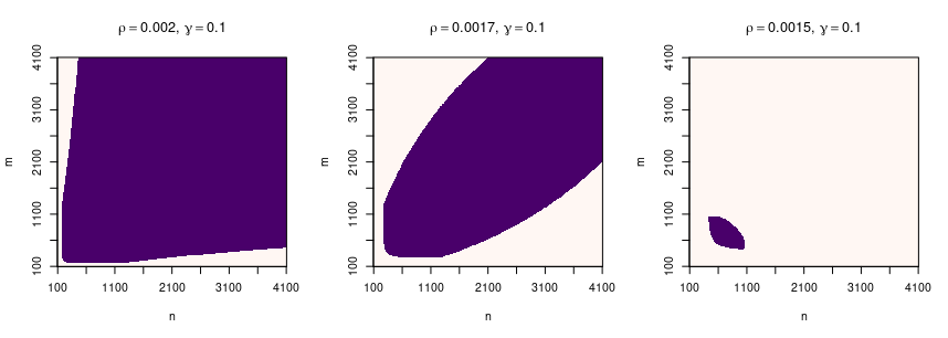
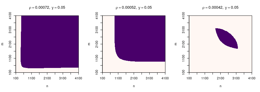
Figure 2: Illustration of the optimality of the least squares estimator for $N=1$. The purple area corresponds to the values of $n$ and $m$, for some fixed values of $\rho$ and $\gamma=K/n=L/m$, for which the lower bound is within a constant factor of the upper bound. More precisely, when $\rho\gamma^{2}\wedge\rho^{2}+\rho(nm)^{-1/2}\wedge\rho^{2}+2\rho^{2}\sqrt{\gamma}$ is larger than half of $\rho\gamma^{2}+(\rho\log K)/(3m)+(\rho\log L)/(3n)+2\rho^{2}\sqrt{\gamma}$. We observe that unless $\rho$ is very small, the upper bound established for the least-squares estimator is within a constant factor of the lower bound for all estimators for most values of $n$ and $m$.

Theorem 4.

Assume that conditionally to $(\boldsymbol{U},\boldsymbol{V})$, the entries $H_{i,j}$ of the observed $n\times m$ matrix $\mathbf{H}$ are independent and drawn from the Binomial distribution with parameter $(N,W^{*}(U_{i},V_{j}))$. There exist universal constants $c,C>0$, such that for any $K,L>C$ satisfying $KL\geqslant L\log^{2}L+K\log^{2}K$ and for any $\rho>0$,

$$\inf_{\widehat{W}}\sup_{W^{*}}\mathbb{E}\big{[}\delta^{2}(\widehat{W},W^{*})\big{]}^{\nicefrac{{1}}{{2}}}\geqslant c\sqrt{\rho}\bigg{(}\frac{KL}{Nnm}\wedge\rho+\frac{1}{N\sqrt{nm}}\wedge\rho\bigg{)}^{\nicefrac{{1}}{{2}}}\!\!\!\!+c\rho\bigg{(}\sqrt{\frac{K}{n}}+\sqrt{\frac{L}{m}}\bigg{)}^{\nicefrac{{1}}{{2}}}\!\!\!\!,$$ (41)

where the inf is over all possible estimators $\widehat{W}$ and the sup is over all $W^{*}\in\mathcal{W}_{\rho}[K,L]$.

The right-hand side of (41) should be compared to (28). One can observe that if the values of $n$,$m$, $K$, $L$ and $\rho$ are such that the dominating term in the upper bound is one of the terms $\rho(K/n)^{1/4}$ and $\rho(L/m)^{1/4}$, then the lower bound in (41) is of the same order as the upper bound. Therefore, in this case, the least squares estimator of the graphon is minimax-rate-optimal. Similarly, if the dominating term is $(\rho KL/(Nnm))^{1/2}$ and $\rho\geqslant KL/(Nnm)$, then the LSE is minimax-rate-optimal. Note also that if $\rho$ is very small, that is smaller than both $KL/(Nnm)$ and $(N^{2}nm)^{-1/2}$, then the lower bound in (41) is of order $\rho$, which might be much smaller than the upper bound established for the LSE. This is not an artifact of the proof, but reflects the fact that in this situation the naive estimator $\widehat{K}\equiv 0$ is better than the LSE. Furthermore, this naive estimator turns out to be minimax-rate-optimal under the mentioned constraint on $\rho$. This basically means that for such small values of $\rho$ the problem of estimating the graphon is not meaningful from a statistical point of view. Figure 2 depicts the regions of the values of $n$ and $m$ where the lower and the upper bounds are of the same order, illustrating thus the optimality of the least-squares estimator. Similarly, Figure 3 shows the regions of the values of $\rho$ and $\gamma=K/n=L/m$, for fixed values of $n$ and $m$, where the lower bound is larger than half of the upper bound. We clearly see that even for very unbalanced graphs ($m$ much larger than $n$), the purple region covers almost the whole square, which means that the least-squares estimator is minimax-rate-optimal in this region.

Figure 3: Illutration of the optimality of the least squares estimator. The purple area corresponds to the values of $\rho$ and $\gamma=K/n=L/m$, for some fixed values of $n$ and $m$, for which the lower bound is within a constant factor of the upper bound. We observe that unless $\rho$ is very small, the upper bound and the lower bound for are of the same order.

6 Numerical experiments

In this section, we present the results of some numerical experiments illustrating the behavior of the error of the estimated graphon $\widehat{W}{}^{\sf LS}$ and its dependence on different parameters of the model. We first consider the case of piecewise constant graphons and study the estimation error of the matrix $\boldsymbol{\Theta}^{*}$. We explore the dependence of this error on $n$ for different values of $(\rho,K,L)$ (assuming that $m=n/2$) as well as on the sparsity parameter $\rho$ for different values of $(n,m,K,L)$. We then show the results of the estimation for a Hölder-continuous graphon, when parameters $K$ and $L$ are chosen as functions of $n$ and $m$ respectively, as recommended by our theoretical results.

6.1 Estimation error of the piecewise constant matrix $\boldsymbol{\Theta}^{*}$

We report the results of two different experimental set-ups, referred to as rand-graphon and cos-graphon. The two set-ups differ in the choice of the graphon only. In both cases, the partitions on which the graphon is piecewise constant is the regular partition induced by the rectangles of the form $[(k-1)/K,k/K)\times[(\ell-1)/L,\ell/L)$ for $k\in[K]$ and $\ell\in[L]$. In the rand-graphon set-up, the values of $W^{*}$ are chosen at random between $0$ and $\rho$, while in the cos-graphon set-up, $W^{*}$ is defined as

$$W^{*}(u,v)=\frac{2\rho}{3}+\frac{\rho}{3}\cos\big{(}3\pi\lfloor Ku\rfloor\lfloor Lv\rfloor\big{)},\qquad\forall u,v\in[0,1].$$ (42)

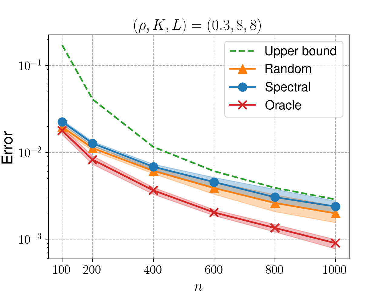
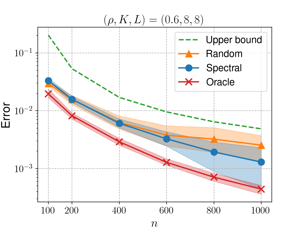
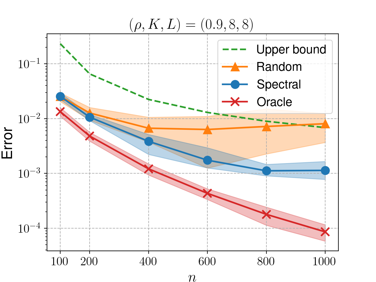
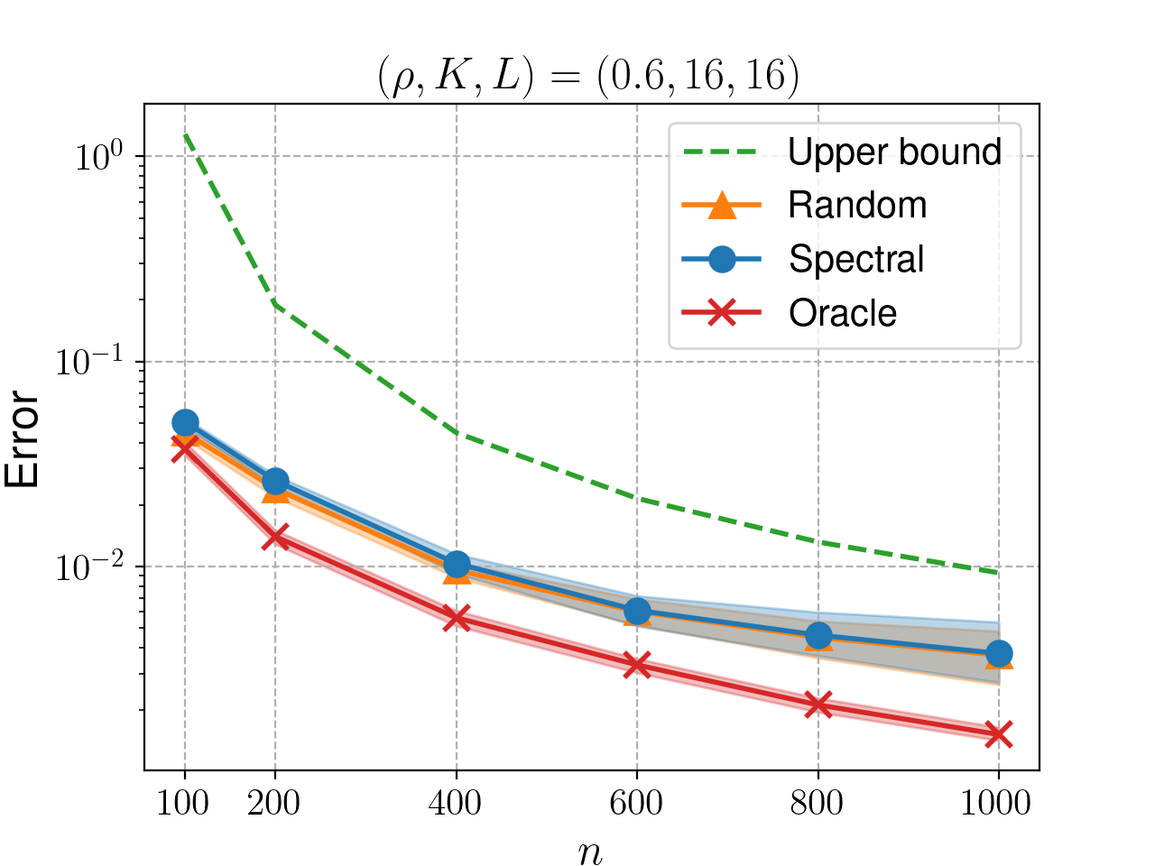
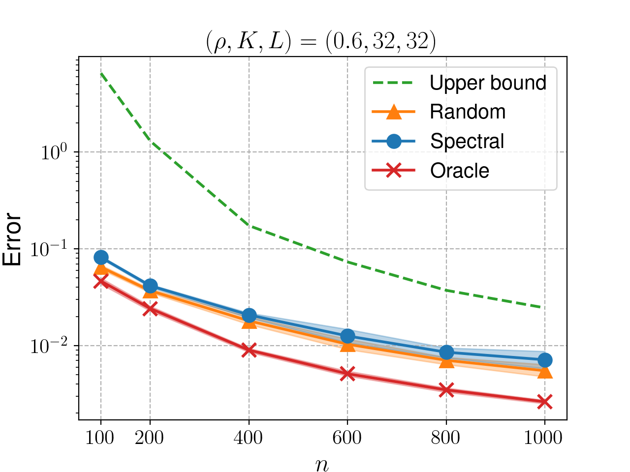
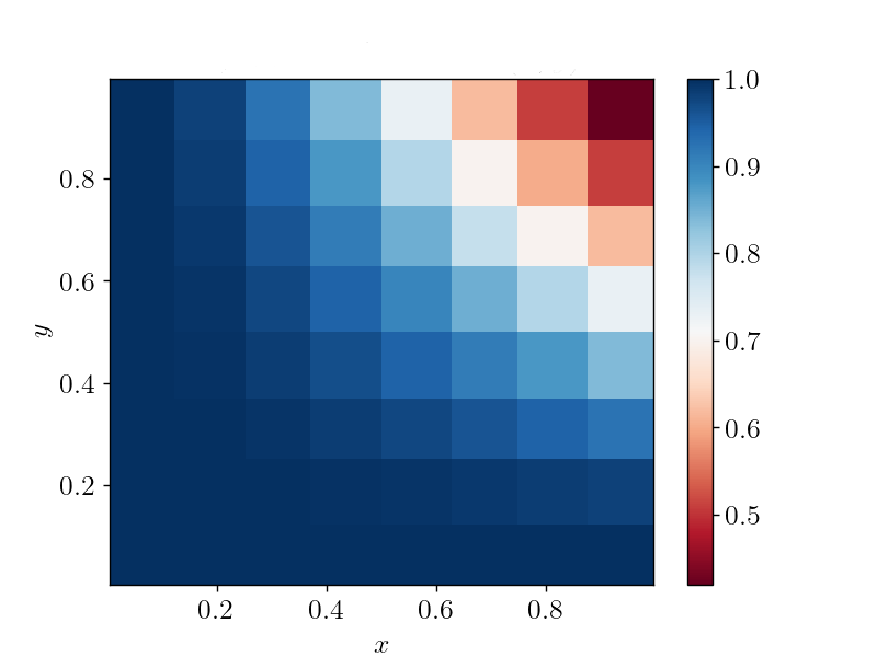
Figure 5: Graphon estimation in the cos-graphon set-up, $W^{*}(x,y)=\frac{2\rho}{3}+\frac{\rho}{3}\cos\big{(}3\pi\lfloor Kx\rfloor\lfloor Ly\rfloor\big{)}$.

The results obtained in these two set-ups are depicted in Figure 4 and Figures 5 and 6, respectively. In each experiment, we chose $m=n/2$ and computed the median of the squared error $\frac{1}{nm}\|\widehat{\boldsymbol{\Theta}}-\boldsymbol{\Theta}^{*}\|^{2}_{\sf F}$ for 50 independent repetitions. The estimator $\widehat{\boldsymbol{\Theta}}$ was computed by Algorithm 1.

For better legibility, the errors in the plots are presented using a log-scale. To check the consistency of the numerical results with our theoretical results, we plotted (in green) the remainder term appearing in the upper-bound in theorem 1. We also displayed the oracle error (red curve) corresponding to the error of the best pseudo-estimator that is built with the knowledge of the true left and right cluster matrices. We only computed the block averages in this case. The labels “spectral” and “random” refer to the initialization process used for the algorithm. To display the uncertainty, we plotted colored areas corresponding to the quantiles of order 0.1 and 0.9 respectively. (One may be surprised by the fact that this area grows with $n$ in some cases; this is an artifact of the log-scale). In Algorithm 1, we chose $\gamma=10^{-3}$ and the maximum number of iterations equal to $40$.

In these experimental results, an evident trend emerges: the error of the “spectral” version consistently diminishes as $n$ increases. Additionally, as $\rho$ assumes larger values and when both $n/K$ and $m/L$ are elevated, the error of the estimator is close to the error of the oracle, a pattern that aligns with intuitive expectations. A larger $\rho$ implies a greater number of links, consequently yielding more accurate estimations. Similarly, heightened values of $n/K$ and $m/L$ correspond to improved accuracy in estimations.

Conversely, the “random” version of the algorithm exhibits a more erratic behavior. In the majority of instances, its error surpasses that of the “spectral” version, particularly when $n/K$ and $m/L$ are large enough.

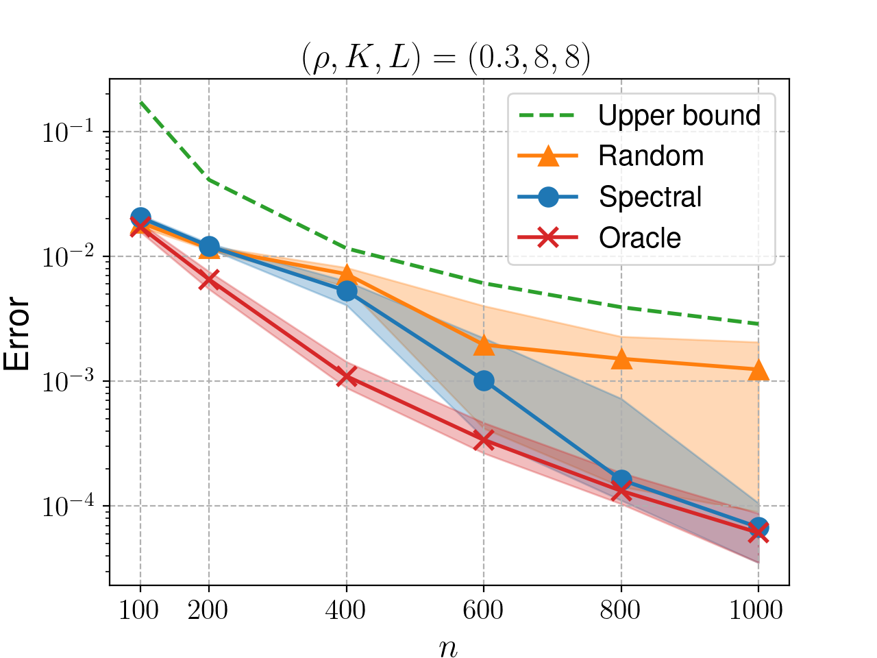
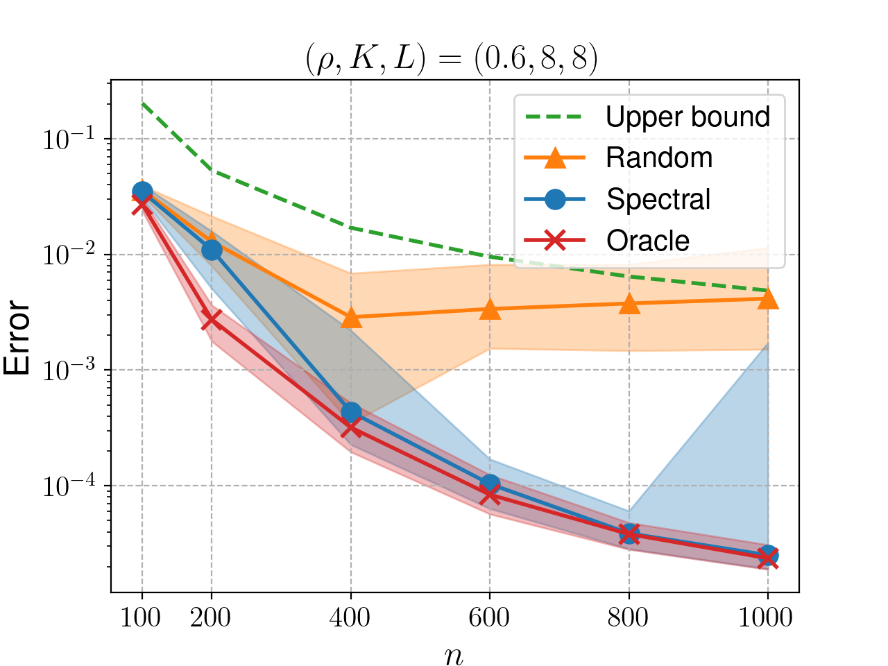
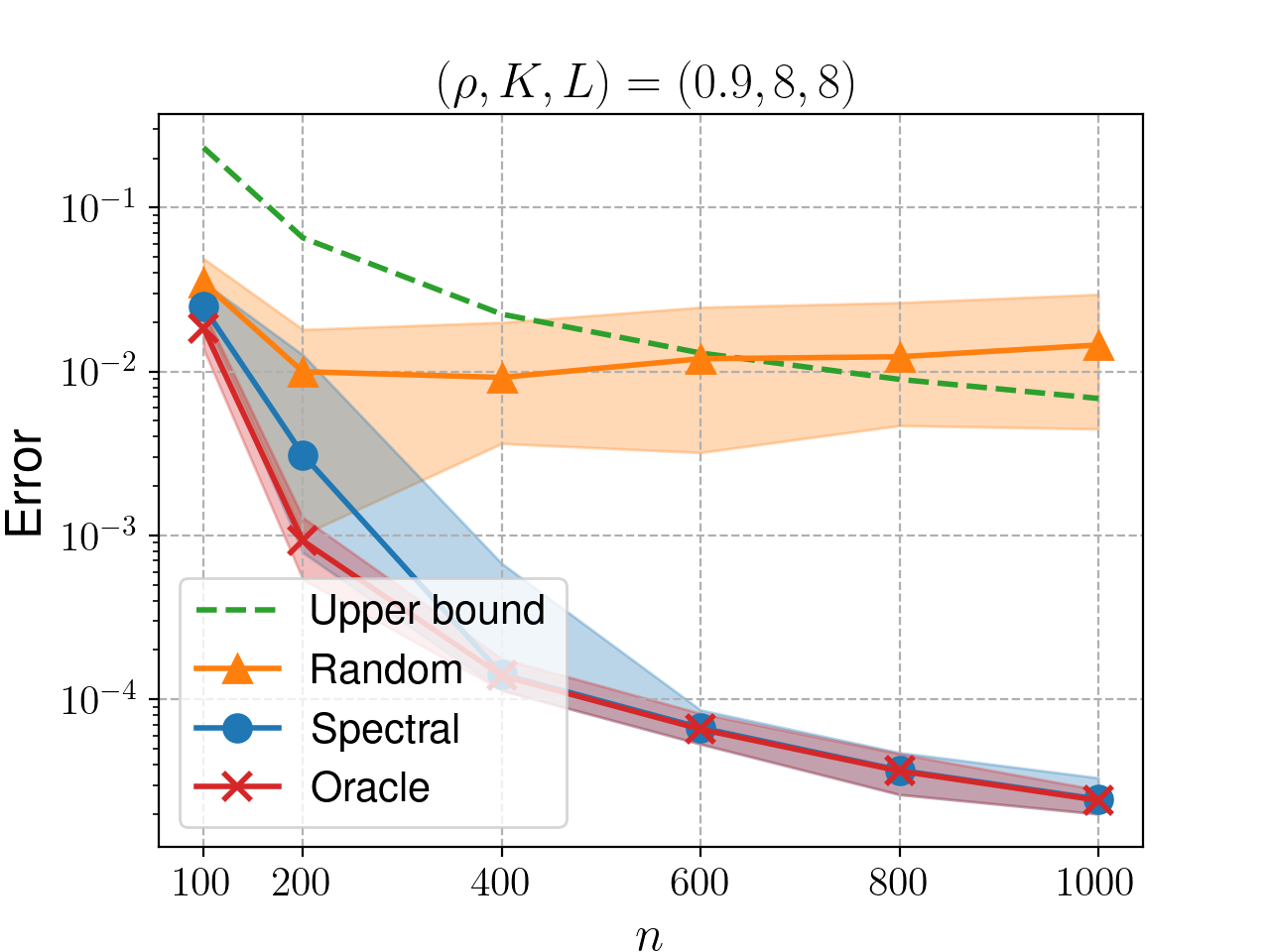
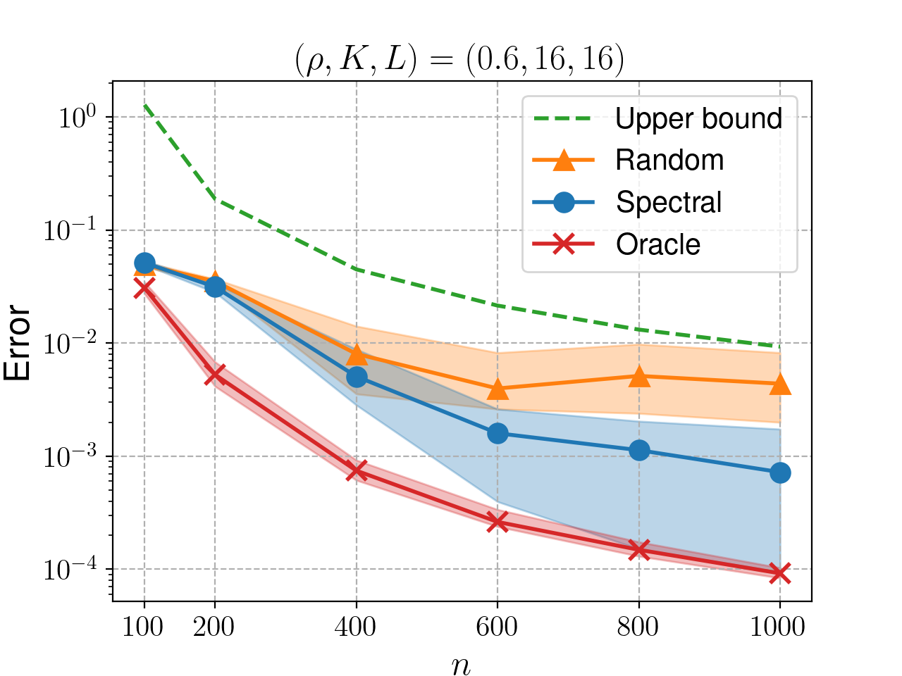
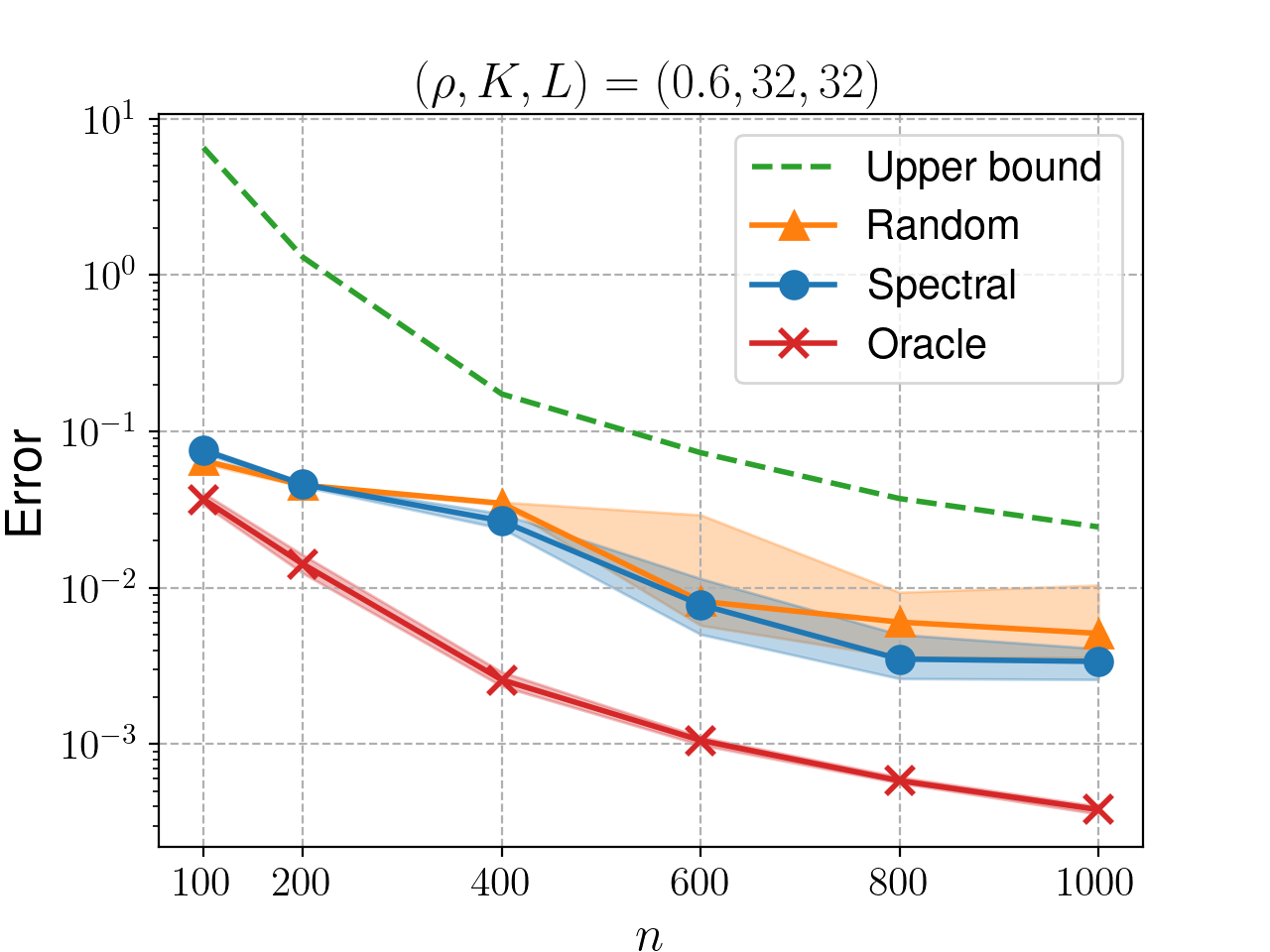
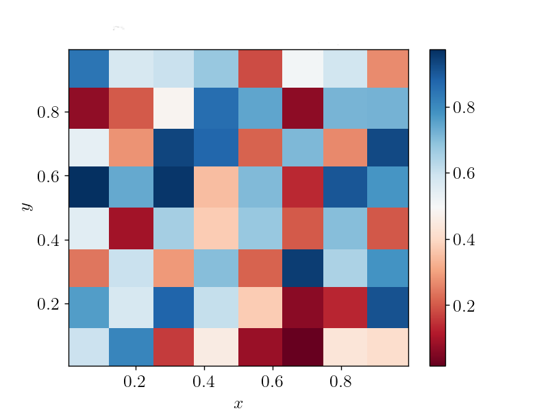
Figure 4: Graphon estimation in the rand-graphon set-up.

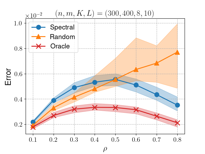
Figure 6: Estimation error as a function of $\rho$, for $W^{*}(x,y)=\frac{2\rho}{3}+\frac{\rho}{3}\cos(3\pi\lfloor Kx\rfloor\lfloor Ly\rfloor)$.

In the set-up of cos-graphon, we displayed in Figure 6 the behavior of the error as a function of $\rho$. For small values of $\rho$, the random initialization appears to be better than the spectral one. Moreover, the error is increasing for $\rho\in[0,\nicefrac{{1}}{{2}}]$ for both initializations. The reason for such a behavior is that the estimator we computed tries to mimic the oracle estimator, which knows the clusters and estimates the matrix $\boldsymbol{\Theta}^{*}$ by computing cluster-wise averages. Thus, if $\boldsymbol{\Theta}^{*}=(\mathbf{Z}^{\textrm{cust}})^{*}\mathbf{Q}^{*}(\mathbf{Z}^{\textrm{prod}})^{*}$, where matrices $(\mathbf{Z}^{\textrm{cust}})^{*}$ and $(\mathbf{Z}^{\textrm{prod}})^{*}$ represent the clusters, then the oracle $\widehat{\boldsymbol{\Theta}}_{o}=(\mathbf{Z}^{\textrm{cust}})^{*}\widehat{\mathbf{Q}}_{o}(\mathbf{Z}^{\textrm{prod}})^{*}$ satisfies

$$\frac{\mathbb{E}\big{[}\|\widehat{\boldsymbol{\Theta}}_{o}-\boldsymbol{\Theta}^{*}\|_{\sf F}^{2}\big{]}}{nm} =\sum_{k,l}\frac{Q_{kl}^{*}(1-Q_{kl}^{*})}{nm}=\sum_{k,l}\frac{\rho\widetilde{Q}_{kl}(1-\rho\widetilde{Q}_{kl})}{nm}=\frac{\rho(\|\widetilde{\mathbf{Q}}\|_{1,1}-\rho\|\widetilde{\mathbf{Q}}\|_{\sf F}^{2})}{nm}$$ (43)

In the above formula, we used the matrix $\widetilde{\mathbf{Q}}=\mathbf{Q}^{*}/\rho$, which has all its entries in $[0,1]$, and denoted by $\|\widetilde{\mathbf{Q}}\|_{1,1}$ the sum of entries of the matrix $\widetilde{\mathbf{Q}}$. The right-hand side of (43) is a function of $\rho$ that increases for $\rho\in[0,\|\widetilde{\mathbf{Q}}\|_{1,1}/2\|\widetilde{\mathbf{Q}}\|^{2}_{\sf F}]$, and decreases outside this interval.

6.2 Estimation error for Hölder-continuous graphons

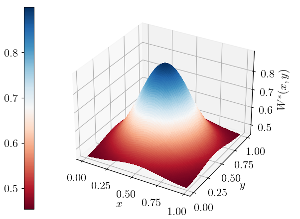
(a) True graphon $W^{*}$

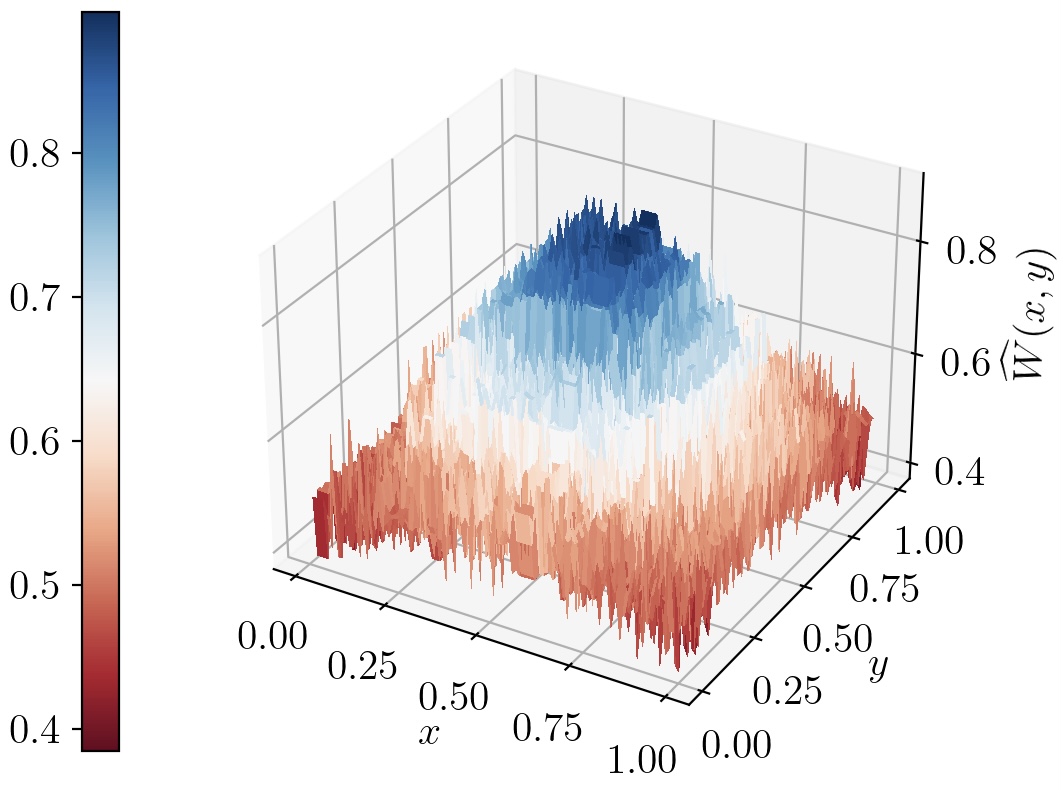
(b) Estimated graphon $\widehat{W}$

Figure 7: Graphon representation for $\rho=0.9$.

To illustrate the behavior of the estimator of the graphon in the case where the latter is Hölder-continuous, we consider the function displayed in Figure 7 and given by

$$W^{*}(u,v)=\frac{\rho}{2}\Big{(}1+\exp\big{\{}-10\big{(}(u-\nicefrac{{1}}{{2}})^{2}+(v-\nicefrac{{1}}{{2}})^{2}\big{)}\big{\}}\Big{)}.$$ (44)

This function being Lipschitz-continuous, we have $\alpha=1$.

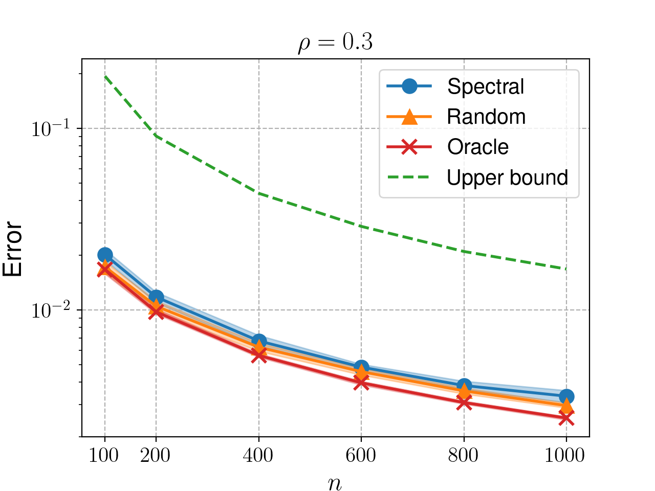
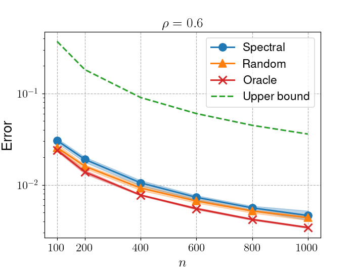
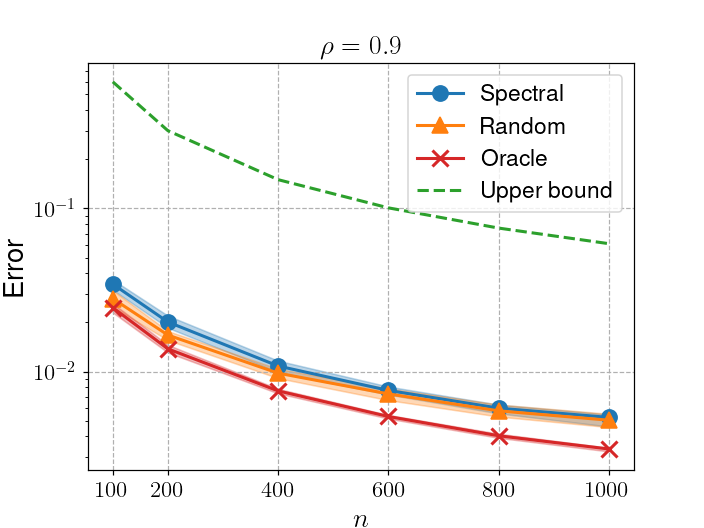
Figure 8: Evolution of the estimation error for a Lipschitz graphon, $m={n}/{2}$.

The average squared error of estimation over 50 repetitions for different values of $n$ and $\rho$ is depicted in Figure 8. Since the true distance $\delta$ is prohibitively hard to compute (because of the minimization over all measure preserving bijections), we computed an approximation of it denoted by $\widetilde{\delta}$. Roughly speaking, $\widetilde{\delta}$ is obtained from $\delta$ by replacing the minimum over all bijections $\tau_{1},\tau_{2}$ by the value of the cost function at the particular instances of bijections, $\tau_{\sigma_{1}}$ and $\tau_{\sigma_{2}}$, used in the proof of 1. More precisely, if $\sigma_{1}$ and $\sigma_{2}$ are permutations of $[n]$ and $[m]$, respectively, such that the sequences $(U_{\sigma_{1}^{-1}(i)})_{i\in[n]}$ and $(V_{\sigma_{2}^{-1}(j)})_{j\in[m]}$ are nondecreasing, then

$$\tau_{\sigma_{1}}(u)=\sum_{i=1}^{n}\Big{(}\frac{\sigma_{1}(i)-1}{n}-u-\frac{i-1}{n}\Big{)}\mathds{1}_{[i-1,i)}(nu),\qquad\tau_{\sigma_{1}}(1)=\frac{\sigma_{1}(n)}{n},$$ (45)

$$\tau_{\sigma_{2}}(v)=\sum_{j=1}^{m}\Big{(}\frac{\sigma_{2}(j)-1}{m}-v-\frac{j-1}{m}\Big{)}\mathds{1}_{[j-1,j)}(nu),\qquad\tau_{\sigma_{2}}(1)=\frac{\sigma_{2}(m)}{m}.$$ (46)

Then, we define

$$\widetilde{\delta}^{2}(\widehat{W},W^{*}) =\big{\|}W^{*}\circ(\tau_{\sigma_{1}}\otimes\tau_{\sigma_{2}})-\widehat{W}\|^{2}_{\mathbb{L}_{2}}$$ (47)

$$=\big{\|}W^{*}\|^{2}_{\mathbb{L}_{2}}-2\sum_{i=1}^{n}\sum_{j=1}^{m}\widehat{\Theta}_{ij}\int_{\frac{\sigma_{1}(i)-1}{n}}^{\frac{\sigma_{1}(i)}{n}}\int_{\frac{\sigma_{2}(j)-1}{m}}^{\frac{\sigma_{2}(j)}{m}}W^{*}(x,y)dxdy+\|\widehat{\boldsymbol{\Theta}}\|_{\sf F}^{2}.$$ (48)

In numerical experiments, the integrals appearing in the right-hand side of the last display are approximated by the Riemann sums. In this case also we observe that the error curves obtained by Monte Carlo simulations are of the same shape as those predicted by the theory. Interestingly, and somewhat surprisingly, the random initialization behaves as well as the spectral one. We do not have any explanation for this observation at this stage.

subsection

7 Proofs of results stated in previous sections

7.1 Proof of Theorem 1 (risk bound for $\widehat{\boldsymbol{\Theta}}{}^{\sf LS}$)

Let us define

$$\Pi_{\mathcal{T}}(\boldsymbol{\Theta}^{*})=\arg\min_{\boldsymbol{\Theta}\in\mathcal{T}}\|\boldsymbol{\Theta}-\boldsymbol{\Theta}^{*}\|_{\sf F},$$ (49)

the best approximation of $\boldsymbol{\Theta}^{*}$ in Frobenius norm by a constant-by-block matrix. Note that the matrix $\Pi_{\mathcal{T}}(\boldsymbol{\Theta}^{*})$ has at most $KL$ distinct entries each of which is the average of the entries of a submatrix of $\boldsymbol{\Theta}^{*}$. Since $\widehat{\boldsymbol{\Theta}}=\widehat{\mathbf{Z}}^{\textrm{cust}}\widehat{\mathbf{Q}}(\widehat{\mathbf{Z}}^{\textrm{prod}})^{\top}$ is the least square estimator, we have

$$\big{\|}\mathbf{H}-\widehat{\boldsymbol{\Theta}}\big{\|}_{\sf F}^{2}\leqslant\big{\|}\mathbf{H}-\Pi_{\mathcal{T}}(\boldsymbol{\Theta}^{*})\big{\|}_{\sf F}^{2}.$$ (50)

Let us define the mean-zero “noise” matrix $\mathbf{E}=\mathbf{H}-\mathbb{E}[\mathbf{H}]=\mathbf{H}-\boldsymbol{\Theta}^{*}$ and rewrite (50) in the following form

$$\|\widehat{\boldsymbol{\Theta}}-\boldsymbol{\Theta}^{*}\|_{\sf F}^{2}\leqslant\|\boldsymbol{\Theta}^{*}-\Pi_{\mathcal{T}}(\boldsymbol{\Theta}^{*})^{\prime}.\|_{\sf F}^{2}+2\langle\widehat{\boldsymbol{\Theta}}-\boldsymbol{\Theta}^{*},\mathbf{E}\rangle+2\langle\boldsymbol{\Theta}^{*}-\Pi_{\mathcal{T}}(\boldsymbol{\Theta}^{*}),\mathbf{E}\rangle.$$ (51)

The expectation of $\mathbf{E}$ being zero, the same is true for the last term in the right-hand. We want to bound the expectation of $\langle\widehat{\boldsymbol{\Theta}}-\boldsymbol{\Theta}^{*},\mathbf{E}\rangle$. To this end, we define

$$\widehat{\mathcal{T}}=\left\{\boldsymbol{\Theta}:\,\exists\mathbf{Q}\in\mathbb{R}^{K\times L}\text{ such that }\boldsymbol{\Theta}=\widehat{\mathbf{Z}}^{\textrm{cust}}\mathbf{Q}(\widehat{\mathbf{Z}}^{\textrm{prod}})^{\top}\right\}\subset\mathcal{T},$$ (52)

and let $\Pi_{\widehat{\mathcal{T}}}(\boldsymbol{\Theta}^{*})=\arg\min_{{\boldsymbol{\Theta}\in\widehat{\mathcal{T}}}}\|\boldsymbol{\Theta}-\boldsymbol{\Theta}^{*}\|_{\sf F}$ be the best Frobenius approximation of $\boldsymbol{\Theta}^{*}$ in $\widehat{\mathcal{T}}$. We use the decomposition

$$\langle\widehat{\boldsymbol{\Theta}}-\boldsymbol{\Theta}^{*},\mathbf{E}\rangle=\underbrace{\langle\Pi_{\widehat{\mathcal{T}}}(\boldsymbol{\Theta}^{*})-\boldsymbol{\Theta}^{*},\mathbf{E}\rangle}_{\Xi_{1}}+\underbrace{\langle\widehat{\boldsymbol{\Theta}}-\Pi_{\widehat{\mathcal{T}}}(\boldsymbol{\Theta}^{*}),\mathbf{E}\rangle}_{\Xi_{2}}.$$ (53)

Lemma 1.

Under the conditions of Theorem 1, we have

$$\mathbb{E}(\Xi_{1}) \leqslant\sigma\sqrt{2(n\log K+m\log L+1)}\,\mathbb{E}[\|\widehat{\boldsymbol{\Theta}}-\boldsymbol{\Theta}^{*}\|_{\sf F}^{2}]^{\nicefrac{{1}}{{2}}}+b\rho(n\log K+m\log L+1).$$ (54)

Proof.

The main steps of the proof consist in applying the Bernstein inequality to $\Xi_{1}$ for a fixed $\boldsymbol{\Theta}$ instead of $\Pi_{\widehat{T}}(\boldsymbol{\Theta}^{*})$, using the union bound and then integrating the high-probability bound. For the first step, let $\boldsymbol{\Theta}\in\mathbb{R}^{n\times m}$ satisfy $\Theta_{i,j}\in[0,\rho]$ for every $(i,j)\in[n]\times[m]$. By definition of the inner product, we have $\langle\boldsymbol{\Theta}-\boldsymbol{\Theta}^{*},\mathbf{E}\rangle=\sum_{(i,j)\in[n]\times[m]}(\boldsymbol{\Theta}-\boldsymbol{\Theta}^{*})_{ij}E_{ij}$. The random variables $E_{ij}$ are independent and satisfy the $(\sigma^{2},b)$-Bernstein condition. The $nm$-vector with entries $(\boldsymbol{\Theta}-\boldsymbol{\Theta}^{*})_{ij}$ has an infinity norm bounded by $\rho$. Therefore, the version of the Bernstein inequality stated in Lemma 12 implies that for all $x>0$, we have

$$\mathbb{P}\Big{(}\langle\boldsymbol{\Theta}-\boldsymbol{\Theta}^{*},\mathbf{E}\rangle\geqslant\sqrt{2x}\,\sigma\|\boldsymbol{\Theta}-\boldsymbol{\Theta}^{*}\|_{\sf F}+b\rho x\Big{)}\leqslant e^{-x}.$$ (55)

Let us define $\Omega_{\mathbf{Z},\mathbf{Z}^{\prime}}=\{(\widehat{\mathbf{Z}}^{\textrm{cust}},\widehat{\mathbf{Z}}^{\textrm{prod}})=(\mathbf{Z},\mathbf{Z}^{\prime})\}$, for each pair of matrices $\mathbf{Z}\in\mathcal{Z}_{n,K,n_{0}}$ and $\mathbf{Z}^{\prime}\in\mathcal{Z}_{m,L,m_{0}}$. On the event $\Omega_{\mathbf{Z},\mathbf{Z}^{\prime}}$, the matrix $\Pi_{\widehat{\mathcal{T}}}(\boldsymbol{\Theta}^{*})$ is deterministic and its elements are averages of the elements of $\boldsymbol{\Theta}^{*}$. Hence, $0\leqslant(\Pi_{\widehat{\mathcal{T}}}(\boldsymbol{\Theta}^{*}))_{ij}\leqslant\|\boldsymbol{\Theta}^{*}\|_{\infty}$ and

$$\mathbb{P}\left(\big{\{}\langle\Pi_{\widehat{\mathcal{T}}}(\boldsymbol{\Theta}^{*})-\boldsymbol{\Theta}^{*},\mathbf{E}\rangle\geqslant\sqrt{2x}\,\sigma\|\Pi_{\widehat{\mathcal{T}}}(\boldsymbol{\Theta}^{*})-\boldsymbol{\Theta}^{*}\|_{\sf F}+b\rho x\big{\}}\cap\Omega_{\mathbf{Z},\mathbf{Z}^{\prime}}\right)\leq e^{-x}.$$ (56)

Note also that the cardinality of $\mathcal{Z}_{n,K,n_{0}}$ is at most $K^{n}$. Combining the last display with the union bound, we get

$$\mathbb{P}\Big{(}\langle\Pi_{\widehat{\mathcal{T}}}(\boldsymbol{\Theta}^{*}) -\boldsymbol{\Theta}^{*},\mathbf{E}\rangle\geqslant\sqrt{2x\rho}\,\sigma\|\Pi_{\widehat{\mathcal{T}}}(\boldsymbol{\Theta}^{*})-\boldsymbol{\Theta}^{*}\|_{\sf F}+b\rho\sigma^{2}x\Big{)}$$ (57)

$$\leqslant\sum_{(\mathbf{Z},\mathbf{Z}^{\prime})}\mathbb{P}\left(\big{\{}\langle\Pi_{\widehat{\mathcal{T}}}(\boldsymbol{\Theta}^{*})-\boldsymbol{\Theta}^{*},\mathbf{E}\rangle\geqslant\sqrt{2x}\,\sigma\|\Pi_{\widehat{\mathcal{T}}}(\boldsymbol{\Theta}^{*})-\boldsymbol{\Theta}^{*}\|_{\sf F}+b\rho x\big{\}}\cap\Omega_{\mathbf{Z},\mathbf{Z}^{\prime}}\right)$$ (58)

$$\leqslant K^{n}L^{m}e^{-x},$$ (59)

where in the first inequality in the above display the sum is over $(\mathbf{Z},\mathbf{Z}^{\prime})$ from the set $\mathcal{Z}_{n,K,n_{0}}\times\mathcal{Z}_{m,L,m_{0}}$ and the factor $K^{n}L^{m}$ corresponds to an upper bound on the cardinality of this set. Finally, choosing $x=n\log K+m\log L+t$ for some $t>0$ and using the basic inequality $uv\leqslant\lambda u^{2}+v^{2}/(4\lambda)$ entails

$$\mathbb{P}\left(\Xi_{1}\geqslant\lambda\|\Pi_{\widehat{\mathcal{T}}}(\boldsymbol{\Theta}^{*})-\boldsymbol{\Theta}^{*}\|_{\sf F}^{2}+\Big{(}\frac{\sigma^{2}}{2\lambda}+b\rho\Big{)}(n\log K+m\log L+t)\right)\leqslant e^{-t}\,$$ (60)

for any $\lambda>0$. Lemma 11 below ensures that

$$\mathbb{E}(\Xi_{1}) \leqslant\lambda\mathbb{E}\Big{[}\|\Pi_{\widehat{\mathcal{T}}}(\boldsymbol{\Theta}^{*})-\boldsymbol{\Theta}^{*}\|_{\sf F}^{2}\Big{]}+\Big{(}\frac{\sigma^{2}}{2\lambda}+b\rho\Big{)}(n\log K+m\log L+1)$$ (61)

$$\leqslant\lambda\mathbb{E}\Big{[}\|\widehat{\boldsymbol{\Theta}}-\boldsymbol{\Theta}^{*}\|_{\sf F}^{2}\Big{]}+\Big{(}\frac{\sigma^{2}}{2\lambda}+b\rho\Big{)}(n\log K+m\log L+1).$$ (62)

Optimizing with respect to $\lambda>0$, we get

$$\mathbb{E}(\Xi_{1}) \leqslant\sigma\sqrt{2(n\log K+m\log L+1)}\,\mathbb{E}[\|\widehat{\boldsymbol{\Theta}}-\boldsymbol{\Theta}^{*}\|_{\sf F}^{2}]^{\nicefrac{{1}}{{2}}}+b\rho(n\log K+m\log L+1).$$ (63)

This completes the proof of the lemma. ∎

We now switch to the evaluation of $\mathbb{E}(\Xi_{2})$. To this end, we first notice that

$$\mathbb{E}(\Xi_{2})=\mathbb{E}\big{[}\langle\Pi_{\widehat{\mathcal{T}}}(\mathbf{H})-\Pi_{\widehat{\mathcal{T}}}(\boldsymbol{\Theta}^{*}),\mathbf{E}\rangle\big{]}=\mathbb{E}\big{[}\langle\Pi_{\widehat{\mathcal{T}}}(\mathbf{E}),\mathbf{E}\rangle\big{]}=\mathbb{E}\big{[}\|\Pi_{\widehat{\mathcal{T}}}(\mathbf{E})\|_{\sf F}^{2}\big{]}.$$ (64)

Lemma 2.

Under the conditions of Theorem 1, we have

$$\mathbb{E}\big{[}\|\Pi_{\widehat{\mathcal{T}}}(\mathbf{E})\|_{\sf F}^{2}\big{]}\leqslant 4(b+\sigma^{2})\big{(}3KL+n\log K+m\log L\big{)}\big{(}2\rho+b\psi_{n,m}(n_{0},m_{0})\big{)}.$$ (65)

Proof.

Recall that $\psi_{n,m}(n_{0},m_{0})=\frac{3\log(en/n_{0})}{m_{0}}+\frac{3\log(em/m_{0})}{n_{0}}$. The scheme of the proof is to apply successively Lemma 14 and Lemma 15. We will proceed by vectorizing the matrices in order to work with vectors only. To this end, let us consider an arbitrary bijection

$$\phi:[n]\times[m]\to[nm]\,.$$ (66)

Let $\mathcal{N}$ and $\mathcal{M}$ be partitions of $[n]$ and $[m]$, respectively, satisfying

$$|\mathcal{N}|=K,\quad|\mathcal{M}|=L\qquad\text{and}\qquad\min_{A\in\mathcal{N}}|A|\geqslant n_{0}\quad\min_{B\in\mathcal{M}}|B|\geqslant m_{0}.$$ (67)

We define $\mathcal{N}\times\mathcal{M}=\{A\times B:\,A\in\mathcal{N},\,B\in\mathcal{M}\}$ which is a partition of $[n]\times[m]$ of cardinality $|\mathcal{N}\times\mathcal{M}|=KL$ satisfying $|A\times B|\geqslant n_{0}m_{0}$ for every $A\times B\in\mathcal{N}\times\mathcal{M}$. We denote by $\mathcal{G}$ the family of all partitions $\phi(\mathcal{N}\times\mathcal{M})$, where $\mathcal{N}$ and $\mathcal{M}$ are as above.

Since the entries of $\Pi_{\widehat{\mathcal{T}}}(\mathbf{E})$ are averages of coefficients of $\mathbf{E}$, if we vectorize $\mathbf{E}$ according to the map $\phi$, meaning that we define $(\vec{\mathbf{E}})_{i}=E_{\phi^{-1}(i)}$ for all $i\in[nm]$, we have that

$$\|\Pi_{\widehat{\mathcal{T}}}(\mathbf{E})\|_{\sf F}^{2} \leqslant\max_{G\in\mathcal{G}}\|\Pi_{G}\vec{\mathbf{E}}\|_{2}^{2}$$ (68)

with entries $(\vec{\mathbf{E}})_{i}$ satisfying the assumptions of Lemma 14. So by the union bound on $\mathcal{G}$, we obtain that

$$\|\Pi_{\widehat{\mathcal{T}}}(\mathbf{E})\|_{\sf F}^{2}\leqslant 4\big{(}t+\log(2M|\mathcal{G}|)\big{)}\big{(}2\sigma^{2}+b\max_{G\in\mathcal{G}}\|\Pi_{G}\vec{\mathbf{E}}\|_{\infty}\big{)}$$ (69)

with probability at least $1-0.5e^{-t}$, where $\log M\leqslant KL\log 12\leqslant 2.5KL$.

Let $\mathcal{A}$ be the family of all the cells of the partitions in $\mathcal{G}$, and let $\mathcal{A}_{(s,l)}=\{\phi(A\times B)\in\mathcal{A}:\,|A|=s\text{ and }|B|=l\}$ for $j=(s,l)\in[n]\times[m]$. Define

$$\mathfrak{F}=\frac{\log(4nm)}{n_{0}m_{0}}+\max_{s,l}\frac{\log|\mathcal{A}_{(s,l)}|}{sl}\geqslant\frac{\log(4nm)}{n_{0}m_{0}}+\frac{\log|\mathcal{A}_{(n_{0},m_{0})}|}{n_{0}m_{0}}\geqslant\frac{7}{n_{0}m_{0}},\qquad\forall n,m\geqslant 3.$$ (70)

According to Lemma 15, on an event of probability at least $1-0.5e^{-t}$,

$$\max_{G\in\mathcal{G}}\|\Pi_{G}\vec{\mathbf{E}}\|_{\infty} \leqslant\max_{A\in\mathcal{A}}\frac{1}{|A|}\Big{|}\sum_{\ell\in A}(\vec{\mathbf{E}})_{\ell}\Big{|}\leqslant\sigma\sqrt{2\Big{(}\frac{t}{n_{0}m_{0}}+\mathfrak{F}\Big{)}}+b\Big{(}\frac{t}{n_{0}m_{0}}+\mathfrak{F}\Big{)}$$ (71)

$$\leqslant\sigma\sqrt{2\mathfrak{F}(1+t/7)}+b\mathfrak{F}(1+t/7)$$ (72)

$$\leqslant\sigma\sqrt{2\mathfrak{F}}\,(1+t/14)+b\mathfrak{F}(1+t/7).$$ (73)

Finally, combining (69) and (73), we have that with probability at least $1-e^{-t}$,

$$\|\Pi_{\widehat{\mathcal{T}}}(\mathbf{E})\|_{\sf F}^{2} \leqslant 4\big{(}t+\log(2M|\mathcal{G}|)\big{)}\big{(}2\sigma^{2}+b\sigma\sqrt{2\mathfrak{F}}\,(1+t/14)+b^{2}\mathfrak{F}(1+t/7)\big{)}.$$ (74)

Using Lemma 11, we obtain the following upper bound on the expectation

$$\mathbb{E}\big{[}\|\Pi_{\widehat{\mathcal{T}}}(\mathbf{E})\|_{\sf F}^{2}\big{]} \leqslant 4\big{(}1+\log(2M|\mathcal{G}|)\big{)}\big{(}2\sigma^{2}+b\sigma\sqrt{2\mathfrak{F}}\,(1+1/7)+b^{2}\mathfrak{F}(1+2/7)\big{)}$$ (75)

$$\leqslant\big{(}1+\log(2M|\mathcal{G}|)\big{)}\big{(}9\sigma^{2}+16\mathfrak{F}b^{2}\big{)}.$$ (76)

For any $(s,l)$ such that $n_{0}\leqslant s\leqslant n$ and $m_{0}\leqslant l\leqslant m$, we have $|\mathcal{A}_{(s,l)}|\leqslant\binom{n}{s}\binom{m}{l}$, which implies

$$|\mathcal{A}_{(s,l)}|\leqslant\Big{(}\frac{en}{s}\Big{)}^{s}\Big{(}\frac{em}{l}\Big{)}^{l}.$$ (77)

Therefore, taking the logarithm of the two sides, we get

$$\frac{\log|\mathcal{A}_{(s,l)}|}{sl} \leqslant\frac{\log(en/s)}{l}+\frac{\log(em/l)}{s}\leqslant\frac{\log(en/n_{0})}{m_{0}}+\frac{\log(em/m_{0})}{n_{0}}\,.$$ (78)

This implies that $\mathfrak{F}\leqslant(1/2)\psi_{n,m}(n_{0},m_{0})$. Therefore,

$$\mathbb{E}\big{[}\|\Pi_{\widehat{\mathcal{T}}}(\mathbf{E})\|_{\sf F}^{2}\big{]} \leqslant\big{(}1+\log(2M|\mathcal{G}|)\big{)}\big{(}9\sigma^{2}+8b^{2}\psi_{n,m}(n_{0},m_{0})\big{)}$$ (79)

where $|\mathcal{G}|=|\mathcal{F}|\leqslant K^{n}L^{m}$ and $M\leqslant 12^{KL}$. Taking into account the fact that $K\geqslant 2$ and $L\geqslant 2$, this leads to

$$1+\log(2M|\mathcal{G}|) \leqslant 1+\log 2+KL\log 12+n\log K+m\log L$$ (80)

$$\leqslant 3KL+n\log K+m\log L.$$ (81)

The term $\mathbb{E}\big{[}\|\Pi_{\widehat{\mathcal{T}}}(\mathbf{E})\|_{\sf F}^{2}\big{]}$ is eventually bounded as follows:

$$\mathbb{E}\big{[}\|\Pi_{\widehat{\mathcal{T}}}(\mathbf{E})\|_{\sf F}^{2}\big{]}\leqslant\big{(}3KL+n\log K+m\log L\big{)}\big{(}9\sigma^{2}+8b^{2}\psi_{n,m}(n_{0},m_{0})\big{)}.$$ (82)

This completes the proof of the lemma. ∎

In order to ease notation in the rest of the proof, let us set $A=n\log K+m\log L$. To conclude, we use the bounds on $\Xi_{1}$ and $\Xi_{2}$ obtained in Lemma 1 and Lemma 2, respectively, as well as decompositions (51) and (53). Since $\mathbb{E}[\langle\boldsymbol{\Theta}^{*}-\Pi_{\mathcal{T}}(\boldsymbol{\Theta}^{*}),\mathbf{E}\rangle]=\langle\boldsymbol{\Theta}^{*}-\Pi_{\mathcal{T}}(\boldsymbol{\Theta}^{*}),\mathbb{E}[\mathbf{E}]\rangle=0$, we arrive at

$$\mathbb{E}[\|\widehat{\boldsymbol{\Theta}}-\boldsymbol{\Theta}^{*}\|_{\sf F}^{2}] \leqslant\|\boldsymbol{\Theta}^{*}-\Pi_{\mathcal{T}}\boldsymbol{\Theta}^{*}\|_{\sf F}^{2}+2\mathbb{E}[\Xi_{1}]+2\mathbb{E}[\Xi_{2}]$$ (83)

$$\leqslant\|\boldsymbol{\Theta}^{*}-\Pi_{\mathcal{T}}\boldsymbol{\Theta}^{*}\|_{\sf F}^{2}+2\sigma\sqrt{2(A+1)}\,\mathbb{E}[\|\widehat{\boldsymbol{\Theta}}-\boldsymbol{\Theta}^{*}\|_{\sf F}^{2}]^{\nicefrac{{1}}{{2}}}+2b\rho(A+1)+2\mathbb{E}[\Xi_{2}].$$ (84)

One can check that the last inequality leads to

$$\big{(}\mathbb{E}[\|\widehat{\boldsymbol{\Theta}}-\boldsymbol{\Theta}^{*}\|_{\sf F}^{2}]^{\nicefrac{{1}}{{2}}}-\sigma\sqrt{2(A+1)}\big{)}^{2} \leqslant\|\boldsymbol{\Theta}^{*}-\Pi_{\mathcal{T}}(\boldsymbol{\Theta}^{*})\|_{\sf F}^{2}+2(A+1)(\sigma^{2}+b\rho)+2\mathbb{E}[\Xi_{2}].$$ (85)

This readily yields

$$\mathbb{E}[\|\widehat{\boldsymbol{\Theta}}-\boldsymbol{\Theta}^{*}\|_{\sf F}^{2}]^{\nicefrac{{1}}{{2}}} \leqslant\|\boldsymbol{\Theta}^{*}-\Pi_{\mathcal{T}}(\boldsymbol{\Theta}^{*})\|_{\sf F}+\sigma\sqrt{2(A+1)}+\big{(}2(A+1)(\sigma^{2}+b\rho)+2\mathbb{E}[\Xi_{2}]\big{)}^{\nicefrac{{1}}{{2}}}$$ (86)

$$\leqslant\|\boldsymbol{\Theta}^{*}-\Pi_{\mathcal{T}}(\boldsymbol{\Theta}^{*})\|_{\sf F}+\big{(}(A+1)(8\sigma^{2}+4b\rho)+4\mathbb{E}[\Xi_{2}]\big{)}^{\nicefrac{{1}}{{2}}}$$ (87)

$$\leqslant\|\boldsymbol{\Theta}^{*}-\Pi_{\mathcal{T}}(\boldsymbol{\Theta}^{*})\|_{\sf F}+\big{(}17\sigma^{2}+4b\rho+8b^{2}\psi_{n,m}(n_{0},m_{0})\big{)}^{\nicefrac{{1}}{{2}}}(3KL+A)^{\nicefrac{{1}}{{2}}},$$ (88)

where in the second line we have used the inequality $\sqrt{x}+\sqrt{y}\leqslant\sqrt{2x+2y}$. Finally, under the condition $\psi_{n,m}(n_{0},m_{0})\leqslant(\sigma/b)^{2}$, we get the claim of the theorem.

7.2 Proof of Theorem 3 (risk bound for $\widehat{W}^{\sf LS}$)

First claim: piecewise constant graphon

In view of (11), the fact that $\widehat{W}=W_{\widehat{\boldsymbol{\Theta}}}$ and 1, we have

$$\mathbb{E}[\delta(W_{\widehat{\boldsymbol{\Theta}}},W^{*})^{2}]^{\nicefrac{{1}}{{2}}} \leqslant\frac{\mathbb{E}[\|\widehat{\boldsymbol{\Theta}}-\boldsymbol{\Theta}^{*}\|_{\sf F}^{2}]^{\nicefrac{{1}}{{2}}}}{\sqrt{nm}}+\mathbb{E}[\delta(W_{\boldsymbol{\Theta}^{*}},W^{*})^{2}]^{\nicefrac{{1}}{{2}}}$$ (89)

$$\leqslant\frac{\mathbb{E}[\|\widehat{\boldsymbol{\Theta}}-\boldsymbol{\Theta}^{*}\|_{\sf F}^{2}]^{\nicefrac{{1}}{{2}}}}{\sqrt{nm}}+\frac{\rho}{\sqrt{2}}\,\bigg{(}\sqrt{\frac{K}{n}}+\sqrt{\frac{L}{m}}\bigg{)}^{\nicefrac{{1}}{{2}}}.$$ (90)

Let $\widehat{\mathcal{T}}$ and $\mathcal{T}^{*}$ be the sets of all $n\times m$ matrices with real entries that are constant by block on the same blocks as $\widehat{\boldsymbol{\Theta}}$ and $\boldsymbol{\Theta}^{*}$, respectively. Clearly, $\widehat{\mathcal{T}}$ and $\mathcal{T}^{*}$ are linear subspaces of the space of $n\times m$ real matrices equipped with the scalar product $\langle\mathbf{M}_{1},\mathbf{M}_{2}\rangle=\operatorname{tr}(\mathbf{M}_{1}^{\top}\mathbf{M}_{2})$. Let $\Pi_{\widehat{\mathcal{T}}}$ be the orthogonal projections onto $\widehat{\mathcal{T}}$. We have $\Pi_{\widehat{\mathcal{T}}}\mathbf{H}=\widehat{\boldsymbol{\Theta}}$. Therefore,

$$\|\widehat{\boldsymbol{\Theta}}-\boldsymbol{\Theta}^{*}\|_{\sf F}=\|\Pi_{\widehat{\mathcal{T}}}\mathbf{H}-\boldsymbol{\Theta}^{*}\|_{\sf F} \stackrel{{\scriptstyle\leavevmode\hbox to10.08pt{\vbox to10.08pt{\text{[drawing]}}}}}{{\leqslant}}\|\Pi_{\widehat{\mathcal{T}}}(\mathbf{H}-\boldsymbol{\Theta}^{*})\|_{\sf F}+\|\Pi_{\widehat{\mathcal{T}}}\boldsymbol{\Theta}^{*}-\boldsymbol{\Theta}^{*}\|_{\sf F}$$ (91)

$$\stackrel{{\scriptstyle\leavevmode\hbox to10.08pt{\vbox to10.08pt{\text{[drawing]}}}}}{{\leqslant}}\|\mathbf{H}-\boldsymbol{\Theta}^{*}\|_{\sf F}+\|(\rho/2)\mathbf{1}_{n}\mathbf{1}_{m}^{\top}-\boldsymbol{\Theta}^{*}\|_{\sf F}.$$ (92)

Above, is a consequence of the triangle inequality, whereas follows from the fact that $\Pi_{\widehat{\mathcal{T}}}$ is an orthogonal projection (hence, a contraction) and the matrix $(\rho/2)\mathbf{1}_{n}\mathbf{1}_{m}^{\top}$ belongs to the image of $\Pi_{\widehat{\mathcal{T}}}$. Hence

$$\frac{1}{nm}\mathbb{E}\big{[}\|\widehat{\boldsymbol{\Theta}}-\boldsymbol{\Theta}^{*}\|_{\sf F}^{2}\,\big{|}\,\boldsymbol{U},\boldsymbol{V}\big{]}\leqslant(\sigma+0.5\rho)^{2}.$$ (93)

For every $k\in[K]$ and $\ell\in[L]$, we define $n_{k}=n|a_{k}-a_{k-1}|$, $N_{k}=\#\{i:U_{i}\in[a_{k-1},a_{k}[\}$, $m_{\ell}=m|b_{\ell}-b_{\ell-1}|$ and $M_{\ell}=\#\{j:V_{j}\in[b_{\ell-1},b_{\ell}[\}$. We also define the event $\Omega_{0}=\{N_{k}\geqslant n_{k}/2;M_{\ell}\geqslant m_{\ell}/2\ \text{for all}\ k\in[K]\ \text{and}\ \ell\in[L]\}$. Since the event $\Omega_{0}^{c}$ is $(\boldsymbol{U},\boldsymbol{V})$-measurable, we get

$$\frac{1}{nm}\mathbb{E}\big{[}\|\widehat{\boldsymbol{\Theta}}-\boldsymbol{\Theta}^{*}\|_{\sf F}^{2}\mathds{1}_{\Omega_{0}^{c}}\big{]}=\frac{1}{nm}\mathbb{E}\Big{(}\mathbb{E}\big{[}\|\widehat{\boldsymbol{\Theta}}-\boldsymbol{\Theta}^{*}\|_{\sf F}^{2}\,\big{|}\,\boldsymbol{U},\boldsymbol{V}\big{]}\mathds{1}_{\Omega_{0}^{c}}\Big{)}\leqslant(\sigma+0.5\rho)^{2}\mathbb{P}(\Omega_{0}^{c}).$$ (94)

Using the union bound and the Chernoff inequality, one can check that

$$\mathbb{P}(\Omega_{0}^{c}) \leqslant\sum_{k=1}^{K}\mathbb{P}(N_{k}\leqslant n_{k}/2)+\sum_{\ell=1}^{L}\mathbb{P}(M_{\ell}\leqslant m_{\ell}/2)\leqslant\sum_{k=1}^{K}e^{-n_{k}/8}+\sum_{\ell=1}^{L}e^{-m_{\ell}/8}.$$ (95)

Since we have assumed that $n_{k}\geqslant 8\log(nK)$ and $m_{\ell}\geqslant 8\log(mL)$, we get $\mathbb{P}(\Omega_{0}^{c})\leqslant n^{-1}+m^{-1}$. If the parameters $n_{0}$ and $m_{0}$ used in the definition of the least squares estimator $\widehat{\boldsymbol{\Theta}}$ satisfy $n_{0}=\min_{k}n_{k}/2=n\Delta^{(K)}/2$ and $m_{0}=\min_{\ell}m_{\ell}/2=m\Delta^{(L)}/2$, then on the event $\Omega_{0}$ we ca apply Theorem 1. One can check that $\psi_{n,m}(n_{0},m_{0})=\psi_{n,m}(\Delta^{(K,L)})$. This, in conjunction with the previous inequalities, implies that

$$\frac{\mathbb{E}[\|\widehat{\boldsymbol{\Theta}}-\boldsymbol{\Theta}^{*}\|_{\sf F}^{2}]}{{nm}} =\frac{\mathbb{E}[\|\widehat{\boldsymbol{\Theta}}-\boldsymbol{\Theta}^{*}\|_{\sf F}^{2}\mathds{1}_{\Omega_{0}}]+\mathbb{E}[\|\widehat{\boldsymbol{\Theta}}-\boldsymbol{\Theta}^{*}\|_{\sf F}^{2}\mathds{1}_{\Omega_{0}^{c}}]}{nm}$$ (96)

$$\leqslant\big{(}25\sigma^{2}+4b\rho\big{)}\Big{(}\frac{3KL}{nm}+\frac{\log K}{m}+\frac{\log L}{n}\Big{)}+\frac{(\sigma+0.5\rho)^{2}}{n}+\frac{(\sigma+0.5\rho)^{2}}{m}$$ (97)

$$\leqslant\Big{\{}\big{(}27\sigma^{2}+4b\rho\big{)}^{\nicefrac{{1}}{{2}}}\Big{(}\frac{3KL}{nm}+\frac{\log K}{m}+\frac{\log L}{n}\Big{)}^{\nicefrac{{1}}{{2}}}+\frac{\rho}{2}\sqrt{\frac{1}{n}+\frac{1}{m}}\Big{\}}^{2},$$ (98)

under condition that $\psi_{n,m}(\Delta^{(K,L)})\leqslant(\sigma/b)^{2}$. One can also check that if $K,L\geqslant 2$ and $n,m\geqslant 5$, it holds

$$\frac{1}{n}+\frac{1}{m}\leq\frac{1}{3}\bigg{(}\sqrt{\frac{K}{n}}+\sqrt{\frac{L}{m}}\bigg{)}.$$ (99)

This inequality, combined with (90), completes the proof of the theorem.

Second claim: Hölder continuous graphons

Using (11) and the Minkowski inequality, we get

$$\mathbb{E}[\delta(\widehat{W}{}^{\sf LS},W^{*})^{2}]^{\nicefrac{{1}}{{2}}} =\mathbb{E}[\delta(W_{\widehat{\boldsymbol{\Theta}}{}^{\sf LS}},W^{*})^{2}]^{\nicefrac{{1}}{{2}}}\leqslant\frac{\mathbb{E}[\|\widehat{\boldsymbol{\Theta}}{}^{\sf LS}-\boldsymbol{\Theta}^{*}\|_{\sf F}^{2}]^{\nicefrac{{1}}{{2}}}}{\sqrt{nm}}+\mathbb{E}[\delta(W_{\boldsymbol{\Theta}^{*}},W^{*})^{2}]^{\nicefrac{{1}}{{2}}}.$$ (100)

Let us set

$$K=L=\bigg{\lfloor}\bigg{(}\frac{3nm\mathcal{L}^{2}}{25\sigma^{2}+4b\rho}\bigg{)}^{1/2(\alpha+1)}\bigg{\rfloor}.$$ (101)

In view of (26), we have

$$(K/m)^{2(\alpha+1)}\leqslant\frac{3n\mathcal{L}^{2}}{(25\sigma^{2}+4b\rho)m^{2\alpha+1}}\leqslant\frac{3(\sigma/2b)^{4(\alpha+1)}\wedge 1}{\log^{4}(2n)}.$$ (102)

Let us choose $n_{0}=\lfloor n/K\rfloor$ and $m_{0}=\lfloor m/K\rfloor$. Thanks to (102), we have

$$\frac{m}{K}\geqslant\big{(}\log^{4}(2n)\big{)}^{1/2(\alpha+1)}\geqslant\log 8>2.$$ (103)

This implies that $m_{0}\geqslant 2$ and, therefore $n_{0}\geqslant 2$. Using once again (102), one can check that

$$\frac{6\log(em/2)}{n_{0}}\leqslant\frac{6\log(en/2)}{m_{0}}\leqslant(\sigma/b)^{2}.$$ (104)

This implies that

$$\psi_{n,m}(n_{0},m_{0}) =\frac{3\log(en/n_{0})}{m_{0}}+\frac{3\log(em/m_{0})}{n_{0}}\leqslant\frac{3\log(en/2)}{m_{0}}+\frac{3\log(em/2)}{n_{0}}\leqslant(\sigma/b)^{2}.$$ (105)

Combining Theorem 1, 2 and claim 2 of 1, we arrive at

$$\mathbb{E}\big{[}\delta(\widehat{W}{}^{\sf LS},W^{*})^{2}\big{]}^{\nicefrac{{1}}{{2}}} \leqslant\frac{3\mathcal{L}}{2K^{\alpha}}+\frac{3\mathcal{L}}{2L^{\alpha}}+\big{(}25\sigma^{2}+4b\rho\big{)}^{\nicefrac{{1}}{{2}}}\Big{(}\frac{3KL}{nm}+\frac{\log K}{m}+\frac{\log L}{n}\Big{)}^{\nicefrac{{1}}{{2}}}$$ (106)

$$\qquad+\frac{2\mathcal{L}}{n^{\alpha/2}}+\frac{2\mathcal{L}}{m^{\alpha/2}}$$ (107)

$$\leqslant\frac{3\mathcal{L}}{K^{\alpha}}+\big{(}25\sigma^{2}+4b\rho\big{)}^{\nicefrac{{1}}{{2}}}\Big{(}\frac{3K^{2}}{nm}+\frac{2\log K}{m}\Big{)}^{\nicefrac{{1}}{{2}}}+\frac{4\mathcal{L}}{m^{\alpha/2}}$$ (108)

$$\leqslant\frac{3\mathcal{L}}{K^{\alpha}}+3K\Big{(}\frac{25\sigma^{2}+4b\rho}{3nm}\Big{)}^{\nicefrac{{1}}{{2}}}+\Big{(}\frac{(50\sigma^{2}+8b\rho)\log K}{m}\Big{)}^{\nicefrac{{1}}{{2}}}+\frac{4\mathcal{L}}{m^{\alpha/2}}.$$ (109)

In the last display, replacing $K$ with its expression (102), we get the claim of the theorem.

This work was partially supported by the grant Investissements d’Avenir (ANR-11-IDEX0003/Labex Ecodec/ANR-11-LABX-0047), funding from the European Research Council (ERC) under the European Union’s Horizon 2020 research and innovation programme grant agreement 741467-FIRMNET and the center Hi! PARIS.

8 Proofs of the propositions

8.1 Proof of 1 (approximation error for a graphon)

First claim (piecewise constant graphon)

In what follows, $\lambda$ refers to the Lebesgue measure on $\mathbb{R}$ and $\lambda_{2}$ is the Lebesgue measure on $\mathbb{R}^{2}$. Let $W^{*}$ be a graphon such that for some $K\times L$ matrix $\mathbf{Q}^{*}$ and some sequences $a_{0}<\ldots<a_{K}$, $b_{0}<\ldots<b_{L}$ satisfying $a_{0}=b_{0}=0$ and $a_{K}=b_{L}=1$, we have $W^{*}(u,v)=Q^{*}_{k,\ell}$ for every $u\in[a_{k-1},a_{k})$ and $v\in[b_{\ell-1},b_{\ell})$. Equivalently,

$$W^{*}(u,v)=\sum_{k=1}^{K}\sum_{\ell=1}^{L}\mathbf{Q}_{k,\ell}^{*}\mathds{1}_{[a_{k-1},a_{k})\times[b_{\ell-1},b_{\ell})}(u,v).$$ (110)

Let us also define the “weight” sequences $w_{k}^{(1)}=a_{k}-a_{k-1}$, $w_{\ell}^{(2)}=b_{\ell}-b_{\ell-1}$ and

$$\widehat{w}_{k}^{(1)}=\frac{1}{n}\sum_{i=1}^{n}\mathds{1}_{[a_{k-1},a_{k}[}(U_{i})\qquad\text{and}\qquad\widehat{w}_{\ell}^{(2)}=\frac{1}{m}\sum_{j=1}^{m}\mathds{1}_{[b_{\ell-1},b_{\ell}[}(V_{j}).$$ (111)

Notice that all the four weight sequences $w^{(1)}$, $w^{(2)}$, $\widehat{w}^{(1)}$ and $\widehat{w}^{(2)}$ are positive and sum to one. As proved in (Klopp et al., 2017, p16), there exist two functions $\psi_{1}:[0,1]\to[K]$ and $\psi_{2}:[0,1]\to[L]$ such that

1. For all $k\in[K]$ and $x\in\big{[}a_{k-1},(a_{k-1}+\widehat{w}_{k}^{(1)})\wedge a_{k}\big{)}$, we have $\psi_{1}(x)=k$

2. For all $\ell\in[L]$ and $x\in\big{[}b_{\ell-1},(b_{\ell-1}+\widehat{w}_{\ell}^{(2)})\wedge b_{\ell}\big{)}$, we have $\psi_{2}(x)=\ell$

3. $\lambda(\psi_{1}^{-1}(k))=\widehat{w}_{k}^{(1)}$ for all $k\in[K]$

4. $\lambda(\psi_{2}^{-1}(\ell))=\widehat{w}_{\ell}^{(2)}$ for all $\ell\in[L]$ .

Using these mappings $\psi_{1}$ and $\psi_{2}$, we construct the graphon $W_{\psi}^{*}(u,v)=\mathbf{Q}^{*}_{\psi_{1}(u),\psi_{2}(v)}$ which satisfies $\delta(W_{\boldsymbol{\Theta}^{*}},W_{\psi}^{*})=0$. This leads to

$$\delta^{2}(W_{\boldsymbol{\Theta}^{*}},W^{*})=\delta^{2}(W_{\psi}^{*},W^{*})\leqslant\|W_{\psi}^{*}-W^{*}\|^{2}_{\mathbb{L}_{2}}\leqslant(B-A)^{2}\lambda_{2}\big{(}(u,v):W^{*}_{\psi}(u,v)\neq W^{*}(u,v)\big{)}.$$ (112)

Our choice of $W_{\psi}^{*}$ ensures that $W^{*}(u,v)=W_{\psi}^{*}(u,v)$ except if $u\in\big{[}(a_{k-1}+\widehat{w}_{k}^{(1)})\wedge a_{k},a_{k}\big{)}$ or $v\in\big{[}(b_{\ell-1}+\widehat{w}_{\ell}^{(2)})\wedge b_{\ell},b_{\ell}\big{)}$. This implies that

$$\delta^{2}(W_{\boldsymbol{\Theta}^{*}},W^{*})\leqslant(B-A)^{2}\bigg{(}\sum_{k=1}^{K}(w_{k}^{(1)}-\widehat{w}_{k}^{(1)})_{+}+\sum_{\ell=1}^{L}(w_{\ell}^{(2)}-\widehat{w}_{\ell}^{(2)})_{+}\bigg{)}.$$ (113)

Since $U_{i}$ are i.i.d. random variables uniformly distributed in $[0,1]$, $n\widehat{w}_{k}^{(1)}$ follows the binomial distribution $\mathcal{B}(n,w_{k}^{(1)})$. This implies that $\mathbb{E}[\widehat{w}_{k}^{(1)}]=w_{k}^{(1)}$ for every $k$. Therefore,

$$\mathbb{E}[(w_{k}^{(1)}-\widehat{w}_{k}^{(1)})_{\pm}]=\frac{1}{2}\mathbb{E}[|w_{k}^{(1)}-\widehat{w}_{k}^{(1)}|]\leqslant\bigg{(}\frac{w_{k}^{(1)}(1-w_{k}^{(1)})}{4n}\bigg{)}^{\nicefrac{{1}}{{2}}}\leqslant\frac{(w_{k}^{(1)})^{\nicefrac{{1}}{{2}}}}{2\sqrt{n}}.$$ (114)

A similar upper bound can be obtained for $\mathbb{E}[(w_{\ell}^{(2)}-\widehat{w}_{\ell}^{(2)})_{+}]$. Therefore, combining (113), (114), the Cauchy-Schwarz inequality and the fact that the weights $w^{(1)}$ sum to one, we get

$$\mathbb{E}[\delta^{2}(W_{\boldsymbol{\Theta}^{*}},W^{*})] \leqslant(B-A)^{2}\bigg{(}\sum_{k=1}^{K}\mathbb{E}[(w_{k}^{(1)}-\widehat{w}_{k}^{(1)})_{+}]+\sum_{\ell=1}^{L}\mathbb{E}[(w_{\ell}^{(2)}-\widehat{w}_{\ell}^{(2)})_{+}]\bigg{)}$$ (115)

$$\leqslant\frac{(B-A)^{2}}{2}\bigg{(}\sqrt{\frac{K}{n}}+\sqrt{\frac{L}{m}}\bigg{)}.$$ (116)

We thus conclude the proof by taking the square root of the obtained inequality.

Second claim (Hölder continuous graphon)

To make the subsequent formulae more compact, we set $a_{n}(i)=i/n$ and assume that $\mathcal{L}=1$. We introduce $I_{i}=\big{[}a_{n}(i-1),a_{n}(i)\big{[}$ and $J_{j}=\big{[}a_{m}(j-1),a_{m}(j)\big{[}$. For every positive $k\in\mathbb{N}$, let $\mathfrak{S}_{n}$ be the set of the permutations of $[k]$. For $\sigma\in\mathfrak{S}_{k}$, let $\tau_{\sigma}$ be the specific measure-preserving application

$$\tau_{\sigma}(x) =\sum_{i=1}^{k}\Big{(}\frac{\sigma(i)-1}{k}+x-\frac{i-1}{k}\Big{)}\mathds{1}_{I_{i}}(x)\qquad\forall x\in[0,1[,\qquad\tau_{\sigma}(1)=\frac{\sigma(k)}{k}.$$ (117)

Notice that $\tau_{\sigma}$ corresponds to permutation of intervals $\{I_{i}:i\in[k]\}$ in accordance with $\sigma$.

Using the definition of $\delta$, we have

$$\delta^{2}(W_{\boldsymbol{\Theta}^{*}},W^{*}) \leqslant\inf_{\begin{subarray}{c}\sigma_{1}\in\mathfrak{S}_{n}\\ \sigma_{2}\in\mathfrak{S}_{m}\end{subarray}}\sum_{i\in[n],j\in[m]}\iint_{I_{i}\times J_{j}}\big{(}\Theta^{*}_{ij}-W^{*}(\tau_{\sigma_{1}}(x),\tau_{\sigma_{2}}(y))\big{)}^{2}dxdy$$ (118)

$$=\inf_{\begin{subarray}{c}\sigma_{1}\in\mathfrak{S}_{n}\\ \sigma_{2}\in\mathfrak{S}_{m}\end{subarray}}\sum_{i\in[n],j\in[m]}\iint_{I_{\sigma_{1}(i)}\times J_{\sigma_{2}(j)}}\big{(}\Theta^{*}_{ij}-W^{*}(x,y)\big{)}^{2}dxdy\,.$$ (119)

Let $\sigma_{1}$ be a random permutation satisfying $U_{(\sigma_{1}(i))}=U_{i}$; for example, let $\sigma_{1}$ be such that $U_{\sigma_{1}^{-1}(1)}\leqslant U_{\sigma_{1}^{-1}(2)}\leqslant\dots\leqslant U_{\sigma_{1}^{-1}(n)}$. We choose $\sigma_{2}$ similarly, so that $V_{(\sigma_{2}(j))}=V_{j}$. Recall that $\Theta^{*}_{ij}=W^{*}(U_{i},V_{j})$. Setting $i^{\prime}=\sigma_{1}(i)$, $j^{\prime}=\sigma_{2}(j)$ and applying the triangle inequality, we get

$$|\Theta^{*}_{i,j}-W^{*}(x,y)| =|W^{*}(x,y)-W^{*}(U_{(i^{\prime})},V_{(j^{\prime})})|$$ (120)

$$\leqslant\big{|}W^{*}(x,y)-W^{*}\big{(}a_{n+1}(i^{\prime}),a_{m+1}(j^{\prime})\big{)}\big{|}$$ (121)

$$\qquad+\big{|}W^{*}\big{(}a_{n+1}(i^{\prime}),a_{m+1}(j^{\prime})\big{)}-W^{*}(U_{(i^{\prime})},V_{(j^{\prime})})\Big{|}.$$ (122)

If $(x,y)\in I_{\sigma_{1}(i)}\times J_{\sigma_{2}(j)}=I_{i^{\prime}}\times J_{j^{\prime}}$, as $\big{(}a_{n+1}(i^{\prime}),a_{m+1}(j^{\prime})\big{)}$ belongs to the same set $I_{i^{\prime}}\times J_{j^{\prime}}$, the Hölder property yields

$$\Big{(}W^{*}(x,y)-W^{*}\big{(}a_{n+1}(i^{\prime}),a_{m+1}(j^{\prime})\big{)}\Big{)}^{2}\leqslant\Big{(}\frac{1}{n^{2}}+\frac{1}{m^{2}}\Big{)}^{\alpha}.$$ (123)

For the second term in (122), we use again the Hölder property, which leads to

$$\big{\{}W^{*}\big{(}a_{n+1}(i^{\prime}),a_{m+1}(j^{\prime})\big{)}-W^{*}(U_{(i^{\prime})},V_{(j^{\prime})})\big{\}}^{2}\leqslant\big{\{}\big{|}a_{n+1}(i^{\prime})-U_{(i^{\prime})}\big{|}^{2}+\big{|}a_{m+1}(j^{\prime})-V_{(j^{\prime})}\big{|}^{2}\big{\}}^{\alpha}.$$ (124)

Then, denoting by $\sum_{i,j}$ the double sum $\sum_{i\in[n]}\sum_{j\in[m]}$, we have

$$\mathbb{E}\Bigg{[}\sum_{i,j}\iint_{I_{i^{\prime}}\times J_{j^{\prime}}}\Big{(}\frac{i^{\prime}}{n+1}-U_{(i^{\prime})}\Big{)}^{2}\Bigg{]} =\frac{1}{n}\mathbb{E}\bigg{[}\sum_{i=1}^{n}\Big{(}\frac{i^{\prime}}{n+1}-U_{(i^{\prime})}\Big{)}^{2}\bigg{]}=\frac{1}{n}\mathbb{E}\bigg{[}\sum_{i=1}^{n}\Big{(}\frac{i}{n+1}-U_{(i)}\Big{)}^{2}\bigg{]}$$ (125)

$$\leqslant\max_{i=1,\dots,n}[\mathbf{Var}(U_{(i)})]\leqslant\frac{1}{4n}$$ (126)

where we used the fact that $U_{(i)}$ is drawn from the beta distribution $\beta(i,n+1-i)$. The term with $V_{(j^{\prime})}$ is treated similarly. Combining (119), the Minkowski inequality, (123) and (126), we get

$$\mathbb{E}[\delta^{2}(W_{\boldsymbol{\Theta}^{*}},W^{*})]^{\nicefrac{{1}}{{2}}} \leqslant\Big{(}\frac{1}{n^{2}}+\frac{1}{m^{2}}\Big{)}^{\alpha/2}\!+\mathbb{E}\Bigg{[}\sum_{i,j}\iint_{I_{i^{\prime}}\times J_{j^{\prime}}}\Big{(}\frac{i^{\prime}}{n+1}-U_{(i^{\prime})}\Big{)}^{2}+\Big{(}\frac{j^{\prime}}{m+1}-V_{(j^{\prime})}\Big{)}^{2}\Bigg{]}^{\alpha/2}$$ (127)

$$\leqslant\Big{(}\frac{1}{n^{2}}+\frac{1}{m^{2}}\Big{)}^{\alpha/2}+\Big{(}\frac{1}{4n}+\frac{1}{4m}\Big{)}^{\alpha/2}\leqslant 2\Big{(}\frac{1}{n}+\frac{1}{m}\Big{)}^{\alpha/2}.$$ (128)

This completes the proof.

8.2 Proof of 2 (approximation error for the matrix $\boldsymbol{\Theta}^{*}$)

Without loss of generality, we prove the desired inequality in the case where $K=\lfloor n/n_{0}\rfloor$ and $L=\lfloor m/m_{0}\rfloor$. Indeed, if the inequality is true for some value of $K$, it is necessarily true for any smaller value as well. The same is true for $L$. Furthermore, we assume $\mathcal{L}=1$.

We construct the constant-by-block matrix $\widetilde{\boldsymbol{\Theta}}\in\mathcal{T}$, where $\mathcal{T}$ is defined by (7) as follows. Let $n=n_{0}K+r$ with $0\leqslant r<n_{0}$ and $m=m_{0}L+s$ with $0\leqslant s<m_{0}$. For all $k\in[K]$ and $\ell\in[L]$, set

$$I_{k}=[(k-1)n_{0}+1,(kn_{0})\wedge n] \qquad\text{and}\qquad J_{\ell}=[(\ell-1)m_{0}+1,(\ell m_{0})\wedge m].$$ (129)

The number of integers contained in each set of the form $I_{k}\times J_{\ell}$ is denoted by $n_{k,\ell}$. We set

$$\widetilde{Q}_{k,\ell}=\frac{1}{n_{k,\ell}}\sum_{i\in I_{k},j\in J_{\ell}}W^{*}(U_{(i)},V_{(j)}).$$ (130)

Finally, for every $(i,j)\in[n]\times[m]$, we set

$$\widetilde{\Theta}_{i,j}=\widetilde{Q}_{\lceil\sigma_{U}(i)/n_{0}\rceil,\lceil\sigma_{V}(j)/m_{0}\rceil}=\sum_{k,\ell}\widetilde{Q}_{k,\ell}\mathds{1}_{\{\sigma_{U}(i)\in I_{k}\}}\mathds{1}_{\{\sigma_{V}(j)\in J_{\ell}\}},$$ (131)

where $\sigma_{U}$ (resp. $\sigma_{V}$) is a permutation of $[n]$ (resp. $[m]$) transforming $(U_{i}:i\in[n])$ (resp. $(V_{j}:j\in[m])$) into a nondecreasing sequence. In other terms, $U_{\sigma_{U}(i)}=U_{(i)}$ and $V_{\sigma_{V}(j)}=V_{(j)}$ for all $i$ and $j$. To bound the approximation error we are interested in, note that ($\sum_{k,\ell}$ stands for $\sum_{k\in[K]}\sum_{\ell\in[L]}$)

$$\mathbb{E}\bigg{[}\frac{1}{nm}\|\widetilde{\boldsymbol{\Theta}}-\boldsymbol{\Theta}^{*}\|_{\sf F}^{2}\bigg{]} =\frac{1}{nm}\sum_{k,\ell}\sum_{i:\sigma_{U}(i)\in I_{k}}\sum_{j:\sigma_{V}(j)\in J_{\ell}}\mathbb{E}\big{[}(\widetilde{Q}_{k,\ell}-\Theta^{*}_{ij})^{2}\big{]}$$ (132)

$$=\frac{1}{nm}\sum_{k,\ell}\sum_{i\in I_{k}}\sum_{j\in J_{\ell}}\mathbb{E}\bigg{[}\bigg{(}\frac{1}{n_{k,\ell}}\sum_{i^{\prime}\in I_{k}}\sum_{j^{\prime}\in J_{\ell}}W^{*}(U_{(i^{\prime})},V_{(j^{\prime})})-W^{*}(U_{(i)},V_{(j)})\bigg{)}^{2}\bigg{]}$$ (133)

(Jensen) $$\leqslant\frac{1}{nm}\sum_{k,\ell}\sum_{i\in I_{k}}\sum_{j\in J_{\ell}}\bigg{(}\frac{1}{n_{k,\ell}}\sum_{i^{\prime}\in I_{k}}\sum_{j^{\prime}\in J_{\ell}}\mathbb{E}\Big{[}\big{(}W^{*}(U_{(i^{\prime})},V_{(j^{\prime})})-W^{*}(U_{(i)},V_{(j)})\big{)}^{2}\Big{]}\bigg{)}.$$ (134)

Using the Hölder property and the Jensen inequality we obtain

$$\mathbb{E}\Big{[}\big{(}W^{*}(U_{(i^{\prime})},V_{(j^{\prime})})-W^{*}(U_{(i)},V_{(j)})\big{)}^{2}\Big{]} \leqslant\mathbb{E}\bigg{[}\bigg{\|}\begin{bmatrix}U_{(i^{\prime})}-U_{(i)}\\ V_{(j^{\prime})}-V_{(j)}\end{bmatrix}\bigg{\|}^{2\alpha}\bigg{]}\leqslant\bigg{\{}\mathbb{E}\bigg{[}\bigg{\|}\begin{bmatrix}U_{(i^{\prime})}-U_{(i)}\\ V_{(j^{\prime})}-V_{(j)}\end{bmatrix}\bigg{\|}^{2}\bigg{]}\bigg{\}}^{\alpha}.$$ (135)

Since $|i-i^{\prime}|<n_{0}+1\leqslant(3/2)n_{0}\leqslant(3n)/(2K)$, (Klopp et al., 2017, Lemma 4.10, p27) leads to

$$\mathbb{E}\big{[}|U_{(i^{\prime})}-U_{(i)}|^{2}\big{]}\leqslant 9/(2K)^{2}.$$ (136)

Similarly, $\mathbb{E}\big{[}|V_{(j^{\prime})}-U_{(j)}|^{2}\big{]}\leqslant 9/(2L)^{2}$. Therefore,

$$\mathbb{E}\Big{[}\frac{1}{nm}\|\widetilde{\boldsymbol{\Theta}}-\boldsymbol{\Theta}^{*}\|_{\sf F}^{2}\Big{]}^{\nicefrac{{1}}{{2}}} \leqslant\mathcal{L}\Big{[}\Big{(}\frac{3}{2K}\Big{)}^{2}+\Big{(}\frac{3}{2L}\Big{)}^{2}\Big{]}^{\alpha/2}\leqslant\frac{3\mathcal{L}}{2}\Big{(}\frac{1}{K^{\alpha}}+\frac{1}{L^{\alpha}}\Big{)},$$ (137)

where we have used the inequality $(a+b)^{c}\leqslant a^{c}+b^{c}$ for $a,b\geqslant 0$ and for $c\in(0,1]$.

8.3 Proof of 3 (relaxation to a linear program)

For further reference, we recall that we are interested in solving the problem

$$\min_{\mathbf{Z}\in\mathcal{Z}(n,K,n_{0})}\mathcal{L}(\mathbf{Z},\mathbf{Q},\mathbf{Z}^{\textrm{prod}}).$$ (OPT 1)

First claim (linearization of the cost function)

We have

$$\mathcal{L}(\mathbf{Z},\mathbf{Q},\mathbf{Z}^{\textrm{prod}})-\|\mathbf{H}\|_{\sf F}^{2} =-2\operatorname{tr}(\mathbf{Z}\mathbf{Q}(\mathbf{Z}^{\textrm{prod}})^{\top}\mathbf{H}^{\top})+\operatorname{tr}(\mathbf{Z}\mathbf{Q}(\mathbf{Z}^{\textrm{prod}})^{\top}\mathbf{Z}^{\textrm{prod}}\mathbf{Q}^{\top}\mathbf{Z}^{\top})$$ (138)

$$=-2\operatorname{tr}(\mathbf{Z}\mathbf{Q}(\mathbf{Z}^{\textrm{prod}})^{\top}\mathbf{H}^{\top})+\operatorname{tr}(\mathbf{Q}\mathbf{D}\mathbf{Q}^{\top}\mathbf{Z}^{\top}\mathbf{Z}).$$ (139)

We will show that $\phi(\mathbf{Z})=-2\operatorname{tr}(\mathbf{Z}\mathbf{Q}(\mathbf{Z}^{\textrm{prod}})^{\top}\mathbf{H}^{\top})+\operatorname{tr}(\mathbf{Q}\mathbf{D}\mathbf{Q}^{\top}\mathbf{Z}^{\top}\mathbf{Z})$. We notice that because of the constraint on the rows of $\mathbf{Z}$, its columns are orthogonal, and $\mathbf{Z}^{\top}\mathbf{Z}=\textsf{diag}(n_{k};k\in[K])$, where $n_{k}=\boldsymbol{Z}_{\bullet\,k}^{\top}{\mathbf{1}}_{n}$ is the number of nonzero entries in the $k$-th column of $\mathbf{Z}$. So we get

$$\operatorname{tr}(\mathbf{Q}\mathbf{D}\mathbf{Q}^{\top}\mathbf{Z}^{\top}\mathbf{Z})=\sum_{k=1}^{K}n_{k}\boldsymbol{Q}_{k,\bullet}\mathbf{D}\boldsymbol{Q}_{k,\bullet}^{\top}=\sum_{k=1}^{K}\boldsymbol{Z}_{\bullet\,k}^{\top}{\mathbf{1}}_{n}\,\boldsymbol{Q}_{k,\bullet}\mathbf{D}\boldsymbol{Q}_{k,\bullet}^{\top}.$$ (140)

This completes the proof of the first claim and entails that (OPT 1) is equivalent to

$$\arg\underset{\mathbf{Z}\in\mathcal{Z}(n,K,n_{0})}{\min}\phi(\mathbf{Z}).$$ (OPT 2)

Second claim (characterization of extreme points)

An extreme point of a convex polytope $\mathcal{P}$ is defined as a point in $\mathcal{P}$ that can not be written as a nontrivial convex combination of two elements in $\mathcal{P}$. First, let us prove that any point in $\mathcal{Z}(n,K,n_{0})$ is an extreme point. Let $\mathbf{Z}\in\mathcal{Z}(n,K,n_{0})$, $\lambda\in(0,1)$, $\mathbf{Z}_{1}$ and $\mathbf{Z}_{2}\in\widetilde{\mathcal{Z}}(n,K,n_{0})$ such that

$$\mathbf{Z} =\lambda\mathbf{Z}_{1}+(1-\lambda)\mathbf{Z}_{2}\,.$$ (141)

Fix some $i\in[n]$, because of the constrain on the lines of $\mathbf{Z}$, there exist $j\in[K]$ such that

$$1=Z_{ij}=\lambda(Z_{1})_{ij}+(1-\lambda)(Z_{2})_{ij}\,.$$ (142)

The only way to satisfy (142) is to have $(Z_{1})_{ij}=(Z_{2})_{ij}=1$ because $\lambda\in(0,1)$. Then $(Z_{1})_{i,\bullet}=(Z_{2})_{i,\bullet}=Z_{i,\bullet}$ because of the row constraints. Finally, this holds for each $i\in[n]$, so $\mathbf{Z}=\mathbf{Z}_{1}=\mathbf{Z}_{2}$, which ensures that $\mathbf{Z}$ is an extreme point.

Now it remains to prove that any extreme point of $\widetilde{\mathcal{Z}}(n,K,n_{0})$ has all its entries in $\{0,1\}$. Let $\mathbf{Z}\in\widetilde{\mathcal{Z}}(n,K,n_{0})$ which has at least one entry in $(0,1)$. Let us prove that $\mathbf{Z}$ can not be an extreme point, that is, we can write $\mathbf{Z}$ as a convex combination of two elements in $\widetilde{\mathcal{Z}}(n,K,n_{0})$. The proof uses the next two lemmas.

Lemma 3.

Let $i_{0}\in[n]$ , $k_{0}\in[K]$ such that $Z_{i_{0}k_{0}}\in(0,1)$. Then

1. There exists $k_{0}^{\prime}\in[K]$ such that $Z_{i_{0},k_{0}^{\prime}}\in(0,1)$.

2. Either $\sum_{i=1}^{n}Z_{i,k_{0}}\notin\mathbb{N}$, or there exists $i_{0}^{\prime}\in[n]$ such that $Z_{i_{0}^{\prime}k_{0}}\in(0,1)$.

Proof of Lemma 3.

The proof is a straightforward consequence of the row and column constraints. Indeed, as the sum of the elements of each line is an integer, if a coefficient is not 0 or 1, then there is another coefficient that lives in $(0,1)$ on the same line, which proves $(i)$. Moreover, if $\sum_{i=1}^{n}Z_{i,k_{0}}\in\mathbb{N}$, the same argument gives that there is another coefficient in $(0,1)$ on the column $k_{0}$. ∎

If we see matrix $\mathbf{Z}$ as a bi-adjacency matrix of a bipartite graph $\mathcal{G}$, with weighted edges given by the entries of $\mathbf{Z}$, the next lemma formally says that either $\mathcal{G}$ contains a cycle, or it has a path with extreme points that correspond to a column that sums to a number strictly greater than $n_{0}$ (see Figure 9).

Lemma 4.

Let $\mathbf{Z}\in\widetilde{\mathcal{Z}}(n,K,n_{0})\backslash\{0,1\}^{n\times K}$. There exists $T\geqslant 1$, and two sequences $(i_{t})_{t=1}^{T}$ and $(k_{t})_{t=0}^{T}$ of different indices (with possibly $k_{0}=k_{T}$) such that

1. $Z_{i_{t}k_{t}}\in(0,1)$ for all $1\leqslant t\leqslant T$.

2. $Z_{i_{t+1}k_{t}}\in(0,1)$ for all $0\leqslant t\leqslant T-1$.

3. Either $\sum_{i=1}^{n}Z_{ik_{t}}>n_{0}$ for $t\in\{0,T\}$ (we say that $\mathbf{Z}$ has a dead end path), or $k_{T}=k_{0}$ ($\mathbf{Z}$ has a cycle).

Proof of Lemma 4.

Let us first assume that all columns of $\mathbf{Z}$ sum to some integers. We denote $Z_{i_{1}k_{0}}$ one element of $\mathbf{Z}$ that is in $(0,1)$ According to part $(i)$ of Lemma 3, there exists $k_{1}\neq k_{0}$ such that $Z_{i_{1}k_{1}}\in(0,1)$. Following the same Lemma 3, we can find $i_{2}\neq i_{1}$, and $k_{2}\neq k_{1}$ such that $Z_{i_{2}k_{1}}\in(0,1)$ and $Z_{i_{2}k_{2}}\in(0,1)$ (so $T\geqslant 2$). We iterate the same process until iteration $T$, with $T$ define as the first time at which we have $i_{T}=i_{t_{0}}$ or $k_{T}=k_{t_{0}}$ for some $0\leqslant t_{0}\leqslant T-1$, meaning that we met a row or a column we already had in the previous iterations. Notice that $t_{0}\leqslant T-2$ because we always have $i_{t}\neq i_{t+1}$ and $k_{t}\neq k_{t+1}$. Then we consider the following shifted sequences.

• $i^{\#}=(i_{t+t_{0}-1})_{t=1}^{T-t_{0}}$ and $k^{\#}_{t}=k_{t+t_{0}}$ for $t\in\{0,\dots,T-t_{0}-1\}$ and $k^{\#}_{T-t_{0}}=k_{t_{0}}$ in the case where $i_{T}=i_{t_{0}}$, meaning that we first met a row we already had in the previous iterations. In this case, $t_{0}\geqslant 1$.

• $i^{\#}=(i_{t+t_{0}})_{t=1}^{T-t_{0}}$ and $k^{\#}=(k_{t+t_{0}})_{t=0}^{T-t_{0}}$ in the case where $k_{T}=k_{t_{0}}$ meaning that we first met a column we already had in the previous iterations.

These sequences $i^{\#}$ and $k^{\#}$ satisfy the cycle conditions of the lemma by construction.

Now we assume that there is a column $k_{0}$ which has a sum not in $\mathbb{N}$. Then it has a coordinate $Z_{i_{1}k_{0}}\in(0,1)$. Applying part $(i)$ of Lemma 3 gives $k_{1}\neq k_{0}$ such that $Z_{i_{1}k_{1}}\in(0,1)$.

• If $\sum_{i=1}^{n}Z_{ik_{1}}>n_{0}$, then lemma is proven for $T=1$ and the dead end path setting.

• Else, $\sum_{i=1}^{n}Z_{ik_{1}}=n_{0}$ then we can iterate similarly the previous process until iteration $T$ define as the first time at which we have $i_{T}=i_{t_{0}}$ or $k_{T}=k_{t_{0}}$ for some $0\leqslant t_{0}\leqslant T-2$ or $\sum_{i=1}^{n}Z_{ik_{T}}>n_{0}$. In the first two cases, we consider the shifted sequences $i^{\#}$ and $k^{\#}$ as before, that satisfy the conditions of the lemma. In the last case, the sequences $(i_{t})_{t=1}^{T}$ and $(k_{t})_{t=0}^{T}$ satisfy the desired dead end path conditions.

Notice that $T<+\infty$ because the number of rows and columns is finite. ∎

The end of the proof of 3 is similar to the one in (Peyré and Cuturi, 2019, Prop 3.4), if we see $\mathbf{Z}$ as the bi-adjacency matrix of a bipartite graph. Let us rewrite the proof adapted for our purpose. We introduce

$$\varepsilon_{1} =\underset{k\in[K]}{\min}\Big{\{}\sum_{i=1}^{n}\frac{Z_{i,k}-n_{0}}{2}:\sum_{i=1}^{n}Z_{i,k}>n_{0}\Big{\}}\wedge 1,\quad\varepsilon_{2}=\min_{i,k}\Big{\{}\frac{Z_{ik}}{2}:Z_{ik}>0\Big{\}}$$ (143)

and $\varepsilon_{3}=(1/2)\min_{i,k}\big{\{}1-Z_{ik}:Z_{ik}<1\big{\}}$. So $\varepsilon_{1}$, $\varepsilon_{2}$ and $\varepsilon_{3}$ are positive real numbers. By convention, the minimum of the empty set is $+\infty$. We finally define $\varepsilon=\min(\varepsilon_{1},\varepsilon_{2},\varepsilon_{3})\in(0,1)$. Hence, when we add or subtrack $\varepsilon$ to one entry of $\mathbf{Z}$ that is in $(0,1)$, it remains in $(0,1)$. Moreover, if this entry is in a column that sums to strictly more than $n_{0}$, if we subtract $\varepsilon$ from this entry, the sum of the column remains strictly greater than $n_{0}$. We apply Lemma 4 which gives to sequences $(i_{t})_{t=1}^{T}$ and $(k_{t})_{t=0}^{T}$ that satisfy the conditions of the lemma. Then we define $\mathbf{Z}_{\varepsilon}$ such that (see Figure 9 for a visual construction of $\mathbf{Z}_{\varepsilon}$)

$$(Z_{\varepsilon})_{ij}=\begin{cases}0&\text{ if }\qquad i\neq i_{t}\text{ or }k\neq k_{t}\\ +\varepsilon&\text{ if }\qquad i=i_{t+1},k=k_{t}\qquad\text{ for some }0\leqslant t\leqslant T-1\\ -\varepsilon&\text{ if }\qquad i=i_{t},k=k_{t}\qquad\text{ for some }1\leqslant t\leqslant T\,.\end{cases}$$ (144)

(a) Cylcle

(b) Dead end path

Figure 9: The starting point is depicted as a red square. In the left-hand side illustration, we encounter a row identical to one we previously encountered, akin to the procedure outlined in Lemma 4. Subsequently, we disregard the preceding steps, symbolized by the crossed-out square. This process generates the sequences necessary for the construction of $\mathbf{Z}_{\varepsilon}$. On the right-hand side illustration, we have not encountered any previously encountered lines or columns. Nonetheless, the procedure halts due to the last column summing to a value exceeding $n_{0}$. This occurrence provides the pathway for constructing $\mathbf{Z}_{\varepsilon}$.

The properties of the sequences imply that

• $\mathbf{Z}_{\varepsilon}{\mathbf{1}}_{K}={\bf 0}_{n}$. Indeed, the $i$-th row of $\mathbf{Z}$ sums to 0 when $i\notin\{i_{1},\dots,i_{T}\}$. But if $i=i_{t}$ for some $t\in[T]$, then there is a $+\varepsilon$ on the $k_{t}$-th column, and a $-\varepsilon$ on the $k_{t-1}$-th column, and 0 anywhere else.

• Moreover we have $\mathbf{Z}_{\varepsilon}^{\top}{\mathbf{1}}_{n}=\delta_{\varepsilon}{\mathbf{1}}_{K}$ where $\delta_{\varepsilon}\in\{0,\pm\varepsilon\}$. Indeed, the $k$-th column sums to 0 for $k\notin\{k_{0},\dots,k_{T}\}$. For $k=k_{t}$ with $t\in[T-1]$, then there is a $+\varepsilon$ on the $i_{t+1}$-th row and a $-\varepsilon$ on the $i_{t}$-th row and 0 anywhere else. For $t\in\{0,T\}$ we have two cases. If $k_{T}=k_{0}$, then the $k_{0}$-th column sums to 0. If $k_{T}\neq k_{0}$, there is only a $+\varepsilon$ on the $k_{0}$-th column and only a $-\varepsilon$ on the $k_{T}$-th column.

The choice of $\varepsilon$ ensures that $\mathbf{Z}_{+}=\mathbf{Z}+\mathbf{Z}_{\varepsilon}$ and $\mathbf{Z}_{-}=\mathbf{Z}-\mathbf{Z}_{\varepsilon}$ live in $\widetilde{\mathcal{Z}}(n,K,n_{0})$. Finally, $\displaystyle\mathbf{Z}=(\mathbf{Z}_{+}+\mathbf{Z}_{-})/2$ and $\mathbf{Z}$ can not be an extreme point.

9 Proof of Theorem 4 (lower bounds)

Although the general structure of the proof and some important parts of it are similar to those of the proof of (Klopp et al., 2017, Proposition 3.4), there are some technical differences that are due to the fact that the graphon and the observed matrix are not symmetric. Furthermore, the bounds involve some terms depending on $L$ and $m$, which was not the case in lower bounds proved in the literature.

To get the desired lower bound, we divide the problem into the following three minimax lower bounds

$$\inf_{\widehat{W}}\sup_{W^{*}\in\mathcal{W}_{\rho}[K,L]}\mathbb{E}_{W^{*}}\big{[}\delta^{2}(\widehat{W},W^{*})\big{]} \geqslant c\rho^{2}\Big{(}\sqrt{\frac{K}{n}}+\sqrt{\frac{L}{m}}\Big{)}$$ (145)

$$\inf_{\widehat{W}}\sup_{W^{*}\in\mathcal{W}_{\rho}[K,L]}\mathbb{E}_{W^{*}}\big{[}\delta^{2}(\widehat{W},W^{*})\big{]} \geqslant c\rho\Big{(}\frac{KL}{Nnm}\wedge\rho\Big{)}$$ (146)

$$\inf_{\widehat{W}}\sup_{W^{*}\in\mathcal{W}_{\rho}[2,2]}\mathbb{E}_{W^{*}}\big{[}\delta^{2}(\widehat{W},W^{*})\big{]} \geqslant c\rho\Big{(}\frac{1}{N\sqrt{nm}}\wedge\rho\Big{)}$$ (147)

If these three inequalities hold true, then the desired result will be true with the constant $c/3$. The rest of this section is split into three subsections, each of which contains the proof of one of the inequalities (145), (146) and (147).

9.1 Proof of (145): error due to the unknown partition

Since $(K,n)$ and $(L,m)$ play symmetric roles, we will only prove the lower bound $\rho^{2}\sqrt{{K}/{n}}$. The same arguments will lead to the lower bound $\rho^{2}\sqrt{{L}/{m}}$. As a consequence, we will get the lower bound $\rho^{2}(\sqrt{{K}/{n}}\vee\sqrt{{L}/{m}})\geqslant\rho^{2}(\sqrt{{K}/{n}}+\sqrt{{L}/{m}})/2$.

Without loss of generality, we can assume that $K$ is a multiple of 16. Indeed, by choosing $C>17$, for any $K>17$, setting $K^{\prime}=16\lfloor K/16\rfloor$, the inequality

$$\inf_{\widehat{W}}\sup_{W^{*}\in\mathcal{W}_{\rho}[K^{\prime},L]}\mathbb{E}_{W^{*}}\big{[}\delta^{2}(\widehat{W},W^{*})\big{]}\geqslant c\rho^{2}\sqrt{\frac{K^{\prime}}{n}}$$ (148)

would imply

$$\inf_{\widehat{W}}\sup_{W^{*}\in\mathcal{W}_{\rho}[K,L]}\mathbb{E}_{W^{*}}\big{[}\delta^{2}(\widehat{W},W^{*})\big{]} \geqslant\inf_{\widehat{W}}\sup_{W^{*}\in\mathcal{W}_{\rho}[K^{\prime},L]}\mathbb{E}_{W^{*}}\big{[}\delta^{2}(\widehat{W},W^{*})\big{]}\geqslant\frac{c}{4}\rho^{2}\sqrt{\frac{K}{n}}.$$ (149)

To establish the desired lower bound, we follow the standard recipe (Tsybakov, 2008, Theorem 2.7) consisting in designing a finite set of graphons that has the following two properties: the graphons from this set are well separated when the distance is measured by the metric $\delta^{2}$ and, in the same time, the distributions generated by these graphons are close, which makes it difficult to differentiate them based on the data matrix $\mathbf{H}$.

To define this set, we choose a $K\times L$ matrix $\mathbf{Q}$ with entries from $\{0,\rho\}$ and two positive numbers $\varepsilon,\varepsilon^{\prime}$; conditions on $\mathbf{Q}$, $\varepsilon$ and $\varepsilon^{\prime}$ will be specified later. For any $K\in\mathbb{N}$, define

$$\mathcal{C}^{K}=\Big{\{}\boldsymbol{s}\in\{-1,+1\}^{K}:\sum_{k=1}^{K}s_{k}=0\Big{\}},\quad I_{\boldsymbol{s},\varepsilon}^{a}=\bigg{[}\sum_{k=1}^{a-1}\Big{(}\frac{1}{K}+\varepsilon s_{k}\Big{)},\sum_{k=1}^{a}\Big{(}\frac{1}{K}+\varepsilon s_{k}\Big{)}\bigg{)}$$ (150)

for $a\in[K]$ and $\boldsymbol{s}\in\mathcal{C}^{K}$, with the convention that $\sum_{k=1}^{0}=0$. Similarly, for every $\boldsymbol{t}\in\mathcal{C}^{L}$, we set $J_{\boldsymbol{t},\varepsilon^{\prime}}^{b}=\big{[}\sum_{\ell=1}^{b-1}\big{(}\frac{1}{L}+\varepsilon^{\prime}t_{\ell}\big{)},\sum_{\ell=1}^{b}\big{(}\frac{1}{L}+\varepsilon^{\prime}t_{\ell}\big{)}\big{)}$. The length of an interval $I$ will be denoted by $|I|$. We can now define the class of graphons $W_{\boldsymbol{s},\boldsymbol{t},\varepsilon}$ for each $\boldsymbol{s}\in\mathcal{C}^{K}$ and $\boldsymbol{t}\in\mathcal{C}^{L}$ by

$$W_{\boldsymbol{s},\boldsymbol{t},\varepsilon}(u,v)=\sum_{k=1}^{K}\sum_{\ell=1}^{L}Q_{k,\ell}\mathds{1}_{I_{\boldsymbol{s},\varepsilon}^{k}}(u)\mathds{1}_{J_{\boldsymbol{t},\varepsilon^{\prime}}^{\ell}}(v).$$ (151)

We denote by $\mathbf{P}_{W_{\boldsymbol{s},\boldsymbol{t},\varepsilon}}$ the distribution of $\mathbf{H}=(H_{ij},i\in[n],j\in[m])$, where $\mathbf{H}$ is sampled according to the Binomial model with graphon $W_{\boldsymbol{s},\boldsymbol{t},\varepsilon}$. The next three lemmas, the proofs of which are postponed to the end of this subsection, provide the main technical tools necessary to establish the desired lower bound.

Lemma 5.

If $4K\varepsilon\leqslant 1$, then for all $\boldsymbol{s}$ and $\boldsymbol{s}^{\prime}$ from $\mathcal{C}^{K}$ and all $\boldsymbol{t}\in\mathcal{C}^{L}$, the following inequality $D_{\sf KL}(\mathbf{P}_{W_{\boldsymbol{s},\boldsymbol{t},\varepsilon}}||\mathbf{P}_{W_{\boldsymbol{s}^{\prime},\boldsymbol{t},\varepsilon}})\leqslant 6n(K\varepsilon)^{2}$ holds true.

Lemma 6.

Assume that $K,L$ are large enough integers multiple of 16 and satisfying $KL\geqslant L\log^{2}L+K\log^{2}K$. There exists $\mathbf{B}\in\{-1,1\}^{K\times L}$ satisfying the following two properties.

1. For all $(k_{1},k_{2})\in[K]^{2}$, $k_{1}\neq k_{2}$, and for all $(\ell_{1},\ell_{2})\in[L]^{2}$, $\ell_{1}\neq\ell_{2}$, it holds that

   $$|\langle\mathbf{B}_{k_{1}\,\bullet},\mathbf{B}_{k_{2}\,\bullet}\rangle| \leqslant L/4\qquad\text{and}\qquad|\langle\mathbf{B}_{\bullet\,\ell_{1}},\mathbf{B}_{\bullet\,\ell_{2}}\rangle|\leqslant K/4$$ (152)

2. Let $\pi_{i}:[K/16]\to[K]$ and $\nu_{i}:[L/16]\to[L]$, $i=1,2$ be arbitrary bijections such that either $\mathop{\rm Im}(\pi_{1})\cap\mathop{\rm Im}(\pi_{2})=\varnothing$ or $\mathop{\rm Im}(\nu_{1})\cap\mathop{\rm Im}(\nu_{2})=\varnothing$. Then

   $$\sum_{k=1}^{K/16}\sum_{\ell=1}^{L/16}\big{(}B_{\pi_{1}(k),\nu_{1}(\ell)}-B_{\pi_{2}(k),\nu_{2}(\ell)}\big{)}^{2}\geqslant\frac{KL}{512}.$$ (153)

For each $\boldsymbol{s}\in\mathcal{C}^{K}$, let us define $\mathcal{A}_{\boldsymbol{s}}=\{k\in[K]:s_{k}=1\}$. Notice that $|\mathcal{A}_{\boldsymbol{s}}|=K/2$.

Lemma 7.

Choose $\mathbf{Q}=\mathbf{B}+\mathbf{1}_{K}\mathbf{1}_{L}\!\!\!{}^{\top}$, where $\mathbf{B}$ is given by Lemma 6. Let $\boldsymbol{s}$ and $\boldsymbol{s}^{\prime}$ be two distinct vectors from $\mathcal{C}^{K}$ such that $|\mathcal{A}_{\boldsymbol{s}}\Delta\mathcal{A}_{\boldsymbol{s}^{\prime}}|\geqslant{K}/{4}$. For $\varepsilon^{\prime}=1/(4L)$, for any $K\in\mathbb{N}$, $\varepsilon\in[0,1/(4K)]$ and $\boldsymbol{t}\in\mathcal{C}^{L}$, we have

$$\delta^{2}(W_{\boldsymbol{s},\boldsymbol{t},\varepsilon},W_{\boldsymbol{s}^{\prime},\boldsymbol{t},\varepsilon})\geqslant\frac{\varepsilon K\rho^{2}}{512}.$$ (154)

Lemma 4.4 in (Klopp et al., 2017) implies that there exists a subset $\widetilde{\mathcal{C}}^{K}\subset\mathcal{C}^{K}$ such that $\log|\widetilde{\mathcal{C}}^{K}|\geqslant{K}/{16}$ and $|\mathcal{A}_{\boldsymbol{s}}\triangle\mathcal{A}_{\boldsymbol{s}^{\prime}}|\geqslant{K}/{4}$ for any $\boldsymbol{s}\neq\boldsymbol{s}^{\prime}$ from $\widetilde{\mathcal{C}}^{K}$. We consider the set $\{W_{\boldsymbol{s},\boldsymbol{t},\varepsilon}:\boldsymbol{s}\in\widetilde{\mathcal{C}}^{K}\}$ for a fixed $\boldsymbol{t}\in\mathcal{C}^{L}$ and for $\varepsilon^{-1}=2^{4}\sqrt{6nK}$. In view of Lemma 5 and Lemma 7, for any $\boldsymbol{s},\boldsymbol{s}^{\prime}\in\widetilde{\mathcal{C}}^{K}$ such that $\boldsymbol{s}\neq\boldsymbol{s}^{\prime}$, we have

$$\delta^{2}(W_{\boldsymbol{s},\varepsilon},W_{\boldsymbol{s}^{\prime},\varepsilon}) \geqslant\frac{\rho^{2}}{2^{13}}\sqrt{\frac{K}{6n}}\quad\text{and}\quad D_{\sf KL}(\mathbf{P}_{W_{\boldsymbol{s},\varepsilon}}||\,\mathbf{P}_{W_{\boldsymbol{s}^{\prime},\varepsilon}})\leqslant\frac{1}{16^{2}}K\leqslant\frac{1}{16}\log|\widetilde{\mathcal{C}}^{K}|.$$ (155)

Therefore, we can apply (Tsybakov, 2008, Theorem 2.7) to get

$$\inf_{\widehat{W}}\sup_{W^{*}\in\mathcal{W}_{\rho}[K,L]}\mathbb{E}_{W^{*}}\big{[}\delta^{2}(\widehat{W},W^{*})\big{]}\geqslant c\rho^{2}\sqrt{\frac{K}{n}}\,$$ (156)

for some universal constant $c>0$. This completes the proof of (145), modulo the proofs of three technical lemmas appended below.

Proof of Lemma 5.

One can check that, for every matrix $\mathbf{A}\in[N]^{n\times m}$, and for every $\boldsymbol{s}\in\mathcal{C}^{K}$,

$$\mathbf{P}_{W_{\boldsymbol{s},\boldsymbol{t},\varepsilon}}(\mathbf{H}=\mathbf{A}) =\prod_{i=1}^{n}\prod_{j=1}^{m}\int_{[0,1]^{2}}\binom{N}{A_{ij}}W_{\boldsymbol{s},\boldsymbol{t},\varepsilon}(u_{i},v_{j})^{A_{ij}}(1-W_{\boldsymbol{s},\boldsymbol{t},\varepsilon}(u_{i},v_{j}))^{N-A_{ij}}\,du_{i}\,dv_{j}.$$ (157)

Using the fact that $W_{\boldsymbol{s},\boldsymbol{t},\varepsilon}$ is piecewise constant, we get

$$\mathbf{P}_{W_{\boldsymbol{s},\boldsymbol{t},\varepsilon}}(\mathbf{H}=\mathbf{A}) =\prod_{i,j}\sum_{k=1}^{K}\sum_{\ell=1}^{L}\int_{I_{\boldsymbol{s},\varepsilon}^{k}}\int_{J_{\boldsymbol{t},\varepsilon^{\prime}}^{\ell}}\binom{N}{A_{ij}}Q_{k\ell}^{A_{i,j}}(1-Q_{k\ell})^{N-A_{i,j}}\,du_{i}\,dv_{j}$$ (158)

$$=\prod_{i,j}\sum_{k,\ell}\binom{N}{A_{ij}}Q_{k\ell}^{A_{i,j}}(1-Q_{k\ell})^{N-A_{i,j}}\big{|}I_{\boldsymbol{s},\varepsilon}^{k}\big{|}\cdot\big{|}J_{\boldsymbol{t},\varepsilon^{\prime}}^{\ell}\big{|}$$ (159)

$$=\sum_{\mathbf{K},\mathbf{L}}\prod_{i,j}\binom{N}{A_{ij}}Q_{K_{ij}L_{ij}}^{A_{ij}}(1-Q_{K_{ij}L_{ij}})^{N-A_{ij}}\big{|}I_{\boldsymbol{s},\varepsilon}^{K_{ij}}\big{|}\cdot\big{|}J_{\boldsymbol{t},\varepsilon^{\prime}}^{L_{ij}}\big{|},$$ (160)

where the outer sum of the last line is over all matrices $\mathbf{K}$ and $\mathbf{L}$ having entries respectively in $[K]$ and in $[L]$. Let us define

$$\Psi(\mathbf{K},\mathbf{L},\mathbf{A}) =\prod_{i,j}\binom{N}{A_{ij}}Q_{K_{ij}L_{ij}}^{A_{ij}}(1-Q_{K_{ij}L_{ij}})^{N-A_{ij}},\quad w_{\boldsymbol{s},\boldsymbol{t},\varepsilon}(\mathbf{K},\mathbf{L})=\prod_{i,j}\big{|}I_{\boldsymbol{s},\varepsilon}^{K_{ij}}\big{|}\cdot\big{|}J_{\boldsymbol{t},\varepsilon^{\prime}}^{L_{ij}}\big{|}.$$ (161)

The computations above imply that

$$D_{\sf KL}(\mathbf{P}_{W_{\boldsymbol{s},\boldsymbol{t},\varepsilon}}||\,\mathbf{P}_{W_{\boldsymbol{s}^{\prime},\boldsymbol{t},\varepsilon}}) =\sum_{\mathbf{A}\in\{0,1\}^{n\times m}}\mathbf{P}_{W_{\boldsymbol{s},\boldsymbol{t},\varepsilon}}(\mathbf{H}=\mathbf{A})\,\log\Big{(}\frac{\mathbf{P}_{W_{\boldsymbol{s},\boldsymbol{t},\varepsilon}}(\mathbf{H}=\mathbf{A})}{\mathbf{P}_{W_{\boldsymbol{s}^{\prime},\boldsymbol{t},\varepsilon}}(\mathbf{H}=\mathbf{A})}\Big{)}$$ (162)

$$=\sum_{\mathbf{A},\mathbf{K},\mathbf{L}}\Psi(\mathbf{K},\mathbf{L},\mathbf{A})w_{\boldsymbol{s},\boldsymbol{t},\varepsilon}(\mathbf{K},\mathbf{L})\log\bigg{(}\frac{\sum_{\mathbf{K}^{\prime},\mathbf{L}^{\prime}}\Psi(\mathbf{K}^{\prime},\mathbf{L}^{\prime},\mathbf{A})w_{\boldsymbol{s},\boldsymbol{t},\varepsilon}(\mathbf{K}^{\prime},\mathbf{L}^{\prime})}{\sum_{\mathbf{K}^{\prime},\mathbf{L}^{\prime}}\Psi(\mathbf{K}^{\prime},\mathbf{L}^{\prime},\mathbf{A})w_{\boldsymbol{s}^{\prime},\boldsymbol{t},\varepsilon}(\mathbf{K}^{\prime},\mathbf{L}^{\prime})}\bigg{)}.$$ (163)

It is clear that $w_{\boldsymbol{s},\boldsymbol{t},\varepsilon}(\mathbf{K},\mathbf{L})\geqslant 0$ and $\sum_{\mathbf{K},\mathbf{L}}w_{\boldsymbol{s},\boldsymbol{t},\varepsilon}(\mathbf{K},\mathbf{L})=1$. Since the function $(x,y)\mapsto x\log(x/y)$ is convex, we apply the Jensen inequality to get

$$D_{\sf KL}(\mathbf{P}_{W_{\boldsymbol{s},\boldsymbol{t}\varepsilon}}||\,\mathbf{P}_{W_{\boldsymbol{s}^{\prime},\boldsymbol{t},\varepsilon}}) \leqslant\sum_{\mathbf{A},\mathbf{K},\mathbf{L}}\Psi(\mathbf{K},\mathbf{L},\mathbf{A})w_{\boldsymbol{s},\boldsymbol{t},\varepsilon}(\mathbf{K},\mathbf{L})\log\bigg{(}\frac{\Psi(\mathbf{K},\mathbf{L},\mathbf{A})w_{\boldsymbol{s},\boldsymbol{t},\varepsilon}(\mathbf{K},\mathbf{L})}{\Psi(\mathbf{K},\mathbf{L},\mathbf{A})w_{\boldsymbol{s}^{\prime},\boldsymbol{t},\varepsilon}(\mathbf{K},\mathbf{L})}\bigg{)}$$ (164)

$$=\sum_{\boldsymbol{K},\mathbf{L}}w_{\boldsymbol{s},\boldsymbol{t},\varepsilon}(\mathbf{K},\mathbf{L})\log\bigg{(}\frac{w_{\boldsymbol{s},\boldsymbol{t},\varepsilon}(\mathbf{K},\mathbf{L})}{w_{\boldsymbol{s}^{\prime},\boldsymbol{t},\varepsilon}(\mathbf{K},\mathbf{L})}\bigg{)}.$$ (165)

The last expression can be seen as the Kullback-Leibler divergence between two product distributions on $[K]^{n\times m}\times[L]^{n\times m}$. Since the Kullback-Leibler divergence between product distributions is the sum of Kullback-Leibler divergences, we get

$$\sum_{\mathbf{K},\mathbf{L}}w_{\boldsymbol{s},\boldsymbol{t},\varepsilon}(\mathbf{K},\mathbf{L})\log\bigg{(}\frac{w_{\boldsymbol{s},\boldsymbol{t},\varepsilon}(\mathbf{K},\mathbf{L})}{w_{\boldsymbol{s}^{\prime},\boldsymbol{t},\varepsilon}(\mathbf{K},\mathbf{L})}\bigg{)} =n\sum_{k=1}^{K}\big{|}I_{\boldsymbol{s},\varepsilon}^{k}\big{|}\log\bigg{(}\frac{|I_{\boldsymbol{s},\varepsilon}^{k}|}{|I_{\boldsymbol{s}^{\prime},\varepsilon}^{k}|}\bigg{)}\leqslant n\sum_{k=1}^{K}\frac{\big{(}|I_{\boldsymbol{s},\varepsilon}^{k}|-|I_{\boldsymbol{s}^{\prime},\varepsilon}^{k}|\big{)}^{2}}{|I_{\boldsymbol{s}^{\prime},\varepsilon}^{k}|},$$ (166)

where the last inequality follows from the fact that the Kullback-Leibler divergence does not exceed the chi-square divergence. Since $|I_{\boldsymbol{s}^{\prime},\varepsilon}^{k}|=(1/K)+\varepsilon s^{\prime}_{k}\geqslant(1/K)-\varepsilon\geqslant 3/(4K)$, we get

$$\sum_{\mathbf{K},\mathbf{L}}w_{\boldsymbol{s},\boldsymbol{t},\varepsilon}(\mathbf{K},\mathbf{L})\log\bigg{(}\frac{w_{\boldsymbol{s},\boldsymbol{t},\varepsilon}(\mathbf{K},\mathbf{L})}{w_{\boldsymbol{s}^{\prime},\boldsymbol{t},\varepsilon}(\mathbf{K},\mathbf{L})}\bigg{)} \leqslant n\sum_{k=1}^{K}\frac{(\varepsilon s_{k}-\varepsilon s^{\prime}_{k}\big{)}^{2}}{3/(4K)}\leqslant 6nK^{2}\varepsilon^{2}.$$ (167)

This completes the proof of the lemma. ∎

Proof of Lemma 6.

Let $\boldsymbol{\Xi}$ be a $K\times L$ random matrix with iid Rademacher entries $\xi_{k,\ell}$, i.e, $\mathbf{P}(\xi_{k,\ell}=\pm 1)=1/2$. Then $\langle\boldsymbol{\Xi}_{k_{1}\,\bullet},\boldsymbol{\Xi}_{k_{2}\,\bullet}\rangle=\sum_{\ell=1}^{L}\xi_{k_{1},\ell}\xi_{k_{2},\ell}$. By the Hoeffding inequality

$$\mathbf{P}(|\langle\boldsymbol{\Xi}_{k_{1}\,\bullet},\boldsymbol{\Xi}_{k_{2}\,\bullet}\rangle|\geqslant L/4)\leqslant 2e^{-L/32}\,.$$ (168)

By the union bound, we obtain that for all $k_{1}\neq k_{2}\in[K],|\,\langle\boldsymbol{\Xi}_{k_{1}\,\bullet},\boldsymbol{\Xi}_{k_{2}\,\bullet}\rangle|\leqslant L/4$ with probability larger than $1-2K^{2}e^{-L/32}$, which is larger than $3/4$ for $L\geqslant 480$. Similarly, one checks that

$$\mathbf{P}(\max_{\ell_{1}\neq\ell_{2}}|\langle\boldsymbol{\Xi}_{\bullet,\ell_{1}},\boldsymbol{\Xi}_{\bullet,\ell_{2}}\rangle|\leqslant K/4)>3/4.$$ (169)

Thus, we get

$$\mathbf{P}\Big{(}\max_{\ell_{1}\neq\ell_{2}}|\langle\boldsymbol{\Xi}_{\bullet,\ell_{1}},\boldsymbol{\Xi}_{\bullet,\ell_{2}}\rangle|\leqslant K/4\text{ and }\max_{k_{1}\neq k_{2}}|\langle\boldsymbol{\Xi}_{k_{1},\bullet},\boldsymbol{\Xi}_{k_{2},\bullet}\rangle|\leqslant L/4\Big{)}>1/2.$$ (170)

For the second property stated in the lemma, we fix some $\mathcal{X}_{i},\mathcal{Y}_{i}$ and $\pi_{i},\nu_{i}$ as in the statement and define

$$T(\pi_{1:2},\nu_{1:2},\boldsymbol{\Xi})=\frac{1}{4}\sum_{k=1}^{K/16}\sum_{\ell=1}^{L/16}\big{(}\xi_{\pi_{1}(k),\nu_{1}(\ell)}-\xi_{\pi_{2}(k),\nu_{2}(\ell)}\big{)}^{2}.$$ (171)

Clearly, $T[\pi_{1:2},\nu_{1:2},\boldsymbol{\Xi}]$ is a sum of $KL/2^{8}$ i.i.d Bernouilli random variables with parameter 1/2. Applying again the Hoeffding inequality, we have

$$\mathbf{P}\Big{(}T[\pi_{1:2},\nu_{1:2},\boldsymbol{\Xi}]\leqslant\frac{KL}{2^{11}}\Big{)} =\mathbf{P}\Big{(}\frac{KL}{2^{9}}-T\geqslant\frac{3KL}{2^{11}}\Big{)}\leqslant e^{-{9KL}/{2^{13}}}\,.$$ (172)

There are no more than $(K/16)!^{2}(L/16)!^{2}$ functions $\pi_{1},\pi_{2},\nu_{1},\nu_{2}$ satisfying conditions of ii). Therefore, the union bound implies that with probability at least $1-(K/16)!^{2}(L/16)!^{2}e^{-9KL/2^{13}}$, we have $T[\pi_{1:2},\nu_{1:2},\boldsymbol{\Xi}]\geqslant KL/2^{11}$ for all $\pi_{1},\pi_{2},\nu_{1},\nu_{2}$. Choosing $K$ and $L$ large enough, and using the condition $KL\geqslant K\log^{2}K+L\log^{2}L$, we get that

$$\mathbf{P}\bigg{(}\min_{\pi_{1},\pi_{2},\nu_{1},\nu_{2}}\sum_{k=1}^{K/16}\sum_{\ell=1}^{L/16}\big{(}\xi_{\pi_{1}(k),\nu_{1}(\ell)}-\xi_{\pi_{2}(k),c\nu_{2}(\ell)}\big{)}^{2}\geqslant\frac{KL}{512}\bigg{)}>1/2.$$ (173)

Combining (170) and (173), we get that the probability that the random matrix $\boldsymbol{\Xi}$ satisfies properties i) and ii) is strictly positive. This implies that the set of such matrices is not empty. ∎

Proof of Lemma 7.

Without loss of generality, throughout this proof, we assume that $\rho=1$. Furthermore, since $\boldsymbol{t}$ is fixed, we will often drop it in the notation and write $W_{\boldsymbol{s},\varepsilon}$ instead of $W_{\boldsymbol{s},\boldsymbol{t},\varepsilon}$.

It suffices to prove that for all measure preserving bijections $\tau_{1}:[0,1]\to[0,1]$ and $\tau_{2}:[0,1]\to[0,1]$,

$$\|W_{\boldsymbol{s},\varepsilon}-W_{\boldsymbol{s}^{\prime},\varepsilon}\circ(\tau_{1}\otimes\tau_{2})\|^{2}_{\mathbb{L}_{2}}\geqslant\frac{\varepsilon K}{512}.$$ (174)

If $u\in I_{\boldsymbol{s},\varepsilon}^{k}$ and $u^{\prime}\in I_{\boldsymbol{s},\varepsilon}^{k^{\prime}}$ for some $k,k^{\prime}\in[K]$, then

$$\bigg{|}\int_{0}^{1}(W_{\boldsymbol{s},\varepsilon}(u,v)-1/2)(W_{\boldsymbol{s},\varepsilon}(u^{\prime},v)-1/2)dv\bigg{|} =\bigg{|}\sum_{\ell=1}^{L}(1/L+\varepsilon^{\prime}t_{\ell})\bigg{(}Q_{k,\ell}-\frac{1}{2}\bigg{)}\bigg{(}Q_{k^{\prime},\ell}-\frac{1}{2}\bigg{)}\bigg{|}$$ (175)

$$\leqslant\frac{1}{4L}|\langle\mathbf{B}_{k,\bullet},\mathbf{B}_{k^{\prime},\bullet}\rangle|+\frac{L\varepsilon^{\prime}}{4}\leqslant\frac{1}{8}.$$ (176)

For $k,k^{\prime}\in[K]$, let $\omega_{kk^{\prime}}=\lambda\big{\{}I_{\boldsymbol{s},\varepsilon}^{k}\cap\tau_{1}^{-1}\big{(}I_{\boldsymbol{s}^{\prime},\varepsilon}^{k^{\prime}}\big{)}\big{\}}$ where $\lambda$ is the Lebesgue measure on $\mathbb{R}$ . Notice that $\sum_{k=1}^{K}\omega_{kk^{\prime}}=({1}/{K})+\varepsilon s^{\prime}_{k^{\prime}}$ and $\sum_{k^{\prime}=1}^{K}\omega_{kk^{\prime}}=({1}/{K})+\varepsilon s_{k}$. We also introduce $h_{\boldsymbol{s},k}(v)=W_{\boldsymbol{s},\varepsilon}(u_{\boldsymbol{s},\varepsilon}^{k},v)-1/2$, where $u_{\boldsymbol{s},\varepsilon}^{k}$ is any point from $I_{\boldsymbol{s},\varepsilon}^{k}$. We have

$$\|W_{\boldsymbol{s},\varepsilon}-W_{\boldsymbol{s}^{\prime},\varepsilon}(\tau_{1}\otimes\tau_{2})\|_{\mathbb{L}_{2}}^{2} =\sum_{k=1}^{K}\sum_{k^{\prime}=1}^{K}\omega_{k,k^{\prime}}\|h_{\boldsymbol{s},k}-h_{\boldsymbol{s}^{\prime},k^{\prime}}\circ\tau_{2}\|_{\mathbb{L}_{2}}^{2}.$$ (177)

In view of the fact that $|h_{\boldsymbol{s}^{\prime},k^{\prime}}(v)|=1/2$ for all $v\in[0,1]$ and (176), for any $k^{\prime}\neq k$, we have

$$\|h_{\boldsymbol{s}^{\prime},k^{\prime}}\circ\tau_{2}-h_{\boldsymbol{s}^{\prime},k^{\prime\prime}}\circ\tau_{2}\|_{\mathbb{L}_{2}}^{2} =\|h_{\boldsymbol{s}^{\prime},k^{\prime}}\|_{\mathbb{L}_{2}}^{2}+\|h_{\boldsymbol{s}^{\prime},k^{\prime\prime}}\|_{\mathbb{L}_{2}}^{2}-2\langle h_{\boldsymbol{s}^{\prime},k^{\prime}},h_{\boldsymbol{s}^{\prime},k^{\prime\prime}}\rangle\geqslant 1/2-1/4=1/4.$$ (178)

By the triangle inequality

$$\|h_{\boldsymbol{s},k}-h_{\boldsymbol{s}^{\prime},k^{\prime}}\circ\tau_{2}\|_{\mathbb{L}_{2}}+\|h_{\boldsymbol{s},k}-h_{\boldsymbol{s}^{\prime},k^{\prime\prime}}\circ\tau_{2}\|_{\mathbb{L}_{2}}\geqslant\|h_{\boldsymbol{s}^{\prime},k^{\prime}}\circ\tau_{2}-h_{\boldsymbol{s}^{\prime},k^{\prime\prime}}\circ\tau_{2}\|_{\mathbb{L}_{2}}\geqslant 1/2\,.$$ (179)

As a consequence, for any $k\in[K]$, there exists at most one $k^{\prime}\in[K]$ such that $\|h_{\boldsymbol{s},k}-h_{\boldsymbol{s}^{\prime},k^{\prime}}\circ\tau_{2}\|_{\mathbb{L}_{2}}<1/4$. If such a $k^{\prime}$ exists, we denote it by $\pi(k)$. If it does not exist, we set $\pi(k)=k$. Using the same arguments, for any $k^{\prime}\in[K]$, there is at most one $k\in[K]$ such that $\|h_{\boldsymbol{s},k}-h_{\boldsymbol{s}^{\prime},k^{\prime}}\circ\tau_{2}\|_{\mathbb{L}_{2}}<1/4$. This implies that $\pi$ is injective and then it is a permutation of $[K]$. Furthermore, we get

$$\|W_{\boldsymbol{s},\varepsilon}-W_{\boldsymbol{s}^{\prime},\varepsilon}\circ(\tau_{1}\otimes\tau_{2})\|_{\mathbb{L}_{2}}^{2} \geqslant\frac{1}{16}\sum_{k=1}^{K}\sum_{k^{\prime}\neq\pi(k)}\omega_{k,k^{\prime}}=\frac{1}{16}\sum_{k=1}^{K}(1/K+\varepsilon s_{k}-\omega_{k,\pi(k)})\,.$$ (180)

If the sum $\sum_{k=1}^{K}(1/K+\varepsilon s_{k}-\omega_{k,\pi(k)})$ is larger than $K\varepsilon/16$, then the lemma is proved.

In the sequel, we check that the same is true if $\sum_{k=1}^{K}(1/K+\varepsilon s_{k}-\omega_{k,\pi(k)})<K\varepsilon/16$ as well. Note that the last inequality can be rewritten as $\sum_{k=1}^{K}\omega_{k,\pi(k)}>1-{K\varepsilon}/{16}$. Let us show that the cardinality of the set $A=\{k\in\mathcal{A}_{\boldsymbol{s}}:s^{\prime}_{\pi(k)}>0\text{ and }\omega_{k,\pi(k)}\geqslant 1/K\}$ is at least ${7K}/{16}$. Indeed, notice that because $\omega_{k,k^{\prime}}\leqslant\big{(}1/K+\varepsilon s_{k}\big{)}\wedge\big{(}1/K+\varepsilon s_{k^{\prime}}\big{)}$, $\omega_{k,\pi(k)}\geqslant 1/K$ implies $s_{k}>0$ and $s^{\prime}_{\pi(k)}>0$. Therefore,

$$1-\frac{K\varepsilon}{16} \leqslant\sum_{k=1}^{K}\omega_{k,\pi(k)}=\sum_{k:s_{k}<0}\omega_{k,\pi(k)}+\sum_{k\in A}\omega_{k,\pi(k)}+\sum_{\begin{subarray}{c}k\notin A\\ s_{k}>0\end{subarray}}\omega_{k,\pi(k)}$$ (181)

$$\leqslant\frac{K}{2}\Big{(}\frac{1}{K}-\varepsilon\Big{)}+|A|\Big{(}\frac{1}{K}+\varepsilon\Big{)}+\Big{(}\frac{K}{2}-|A|\Big{)}\frac{1}{K}=1+\varepsilon\Big{(}|A|-\frac{K}{2}\Big{)},$$ (182)

which leads to $|A|\geqslant 7K/16$.

Since $\boldsymbol{s},\boldsymbol{s}^{\prime}\in\widetilde{\mathcal{C}}^{K}$ are such that $|\mathcal{A}_{\boldsymbol{s}}\triangle\mathcal{A}_{\boldsymbol{s}^{\prime}}|\geqslant K/4$, we have $|\mathcal{A}_{\boldsymbol{s}}\cap\mathcal{A}_{\boldsymbol{s}^{\prime}}|\leqslant{3K}/{8}$. Let us choose $B\subset A\cap\mathcal{A}_{\boldsymbol{s}^{\prime}}^{c}$ of cardinality $K/16$ and set $C=\pi(B)$. Such a choice is possible since

$$|A\cap\mathcal{A}_{\boldsymbol{s}^{\prime}}^{c}|=|A|-|A\cap\mathcal{A}_{\boldsymbol{s}^{\prime}}|\geqslant\frac{7K}{16}-|\mathcal{A}_{\boldsymbol{s}}\cap\mathcal{A}_{\boldsymbol{s}^{\prime}}|\geqslant\frac{7K}{16}-\frac{3K}{8}=\frac{K}{16}.$$ (183)

Note also that $B\cap C=\varnothing$. Indeed, if $k\in B$, then $\pi(k)\in\mathcal{A}_{\boldsymbol{s}^{\prime}}$. Therefore, $\pi(k)\notin B$ meaning that $k\notin C$.

For $\ell,\ell^{\prime}\in[L]$, let $\omega^{\prime}_{\ell,\ell^{\prime}}=\lambda\big{\{}J_{\boldsymbol{t},\varepsilon^{\prime}}^{\ell}\cap\tau_{2}^{-1}(J_{\boldsymbol{t},\varepsilon^{\prime}}^{\ell^{\prime}})\big{\}}$. Using the same arguments as above, we obtain the existence of a permutation $\nu:[L]\to[L]$ such that, akin to (180),

$$\|W_{\boldsymbol{s},\varepsilon}-W_{\boldsymbol{s}^{\prime},\varepsilon}\circ(\tau_{1}\otimes\tau_{2})\|_{\mathbb{L}_{2}}^{2} \geqslant\frac{1}{16}\sum_{b=1}^{L}(1/L+\varepsilon^{\prime}t_{\ell}-\omega^{\prime}_{\ell,\nu(\ell)}).$$ (184)

Define the set $A^{\prime}=\{\ell\in[L]:t_{\ell}>0,\omega^{\prime}_{\ell,\nu(\ell)}\geqslant 1/L\}$. If $|A^{\prime}|\leqslant L/16$, then

$$\sum_{\ell=1}^{L}(1/L+\varepsilon^{\prime}t_{\ell}-\omega^{\prime}_{\ell,\nu(\ell)}) \geqslant 1-\sum_{t_{\ell}<0}\omega^{\prime}_{\ell,\nu(\ell)}-\sum_{t_{\ell}>0}\omega^{\prime}_{\ell,\nu(\ell)}(\mathds{1}_{\ell\notin A^{\prime}}+\mathds{1}_{\ell\in A^{\prime}})$$ (185)

$$\geqslant 1-\frac{L}{2}\Big{(}\frac{1}{L}-\varepsilon^{\prime}\Big{)}-\Big{(}\frac{L}{2}-|A^{\prime}|\Big{)}\frac{1}{L}-|A^{\prime}|\Big{(}\frac{1}{L}+\varepsilon^{\prime}\Big{)}=\Big{(}\frac{L}{2}-|A^{\prime}|\Big{)}\varepsilon^{\prime}$$ (186)

$$\geqslant\frac{7L\varepsilon^{\prime}}{16}\geqslant 1/16$$ (187)

and therefore $\|W_{\boldsymbol{s},\varepsilon}-W_{\boldsymbol{s}^{\prime},\varepsilon}\circ(\tau_{1}\otimes\tau_{2})\|_{\mathbb{L}_{2}}^{2}\geqslant 1/256\geqslant K\varepsilon/64$, where we used that $4K\varepsilon<1$.

Suppose now that $|A^{\prime}|>L/16$. Let $B^{\prime}$ be an arbitrary subset of $A^{\prime}$ of cardinality $L/16$. We have

$$\|W_{\boldsymbol{s},\varepsilon}-W_{\boldsymbol{s}^{\prime},\varepsilon}\circ(\tau_{1}\otimes\tau_{2})\|_{\mathbb{L}_{2}}^{2} \geqslant\sum_{k\in B}\sum_{\ell\in B^{\prime}}\int_{I_{\boldsymbol{s},\varepsilon}^{k}\times J_{\boldsymbol{s}^{\prime},\varepsilon}^{\ell}}\big{(}W_{\boldsymbol{s},\varepsilon}-W_{\boldsymbol{s}^{\prime},\varepsilon}(\tau_{1}\otimes\tau_{2})\big{)}^{2}(u,v)\,du\,dv$$ (188)

$$\geqslant\sum_{k\in B}\sum_{\ell\in B^{\prime}}\omega_{k,\pi(k)}\omega^{\prime}_{\ell,\nu(\ell)}(Q_{k,\ell}-Q_{\pi(k),\nu(\ell)})^{2}$$ (189)

$$\geqslant\frac{1}{4KL}\sum_{k\in B}\sum_{\ell\in B^{\prime}}(B_{k,\ell}-B_{\pi(k),\nu(\ell)})^{2}.$$ (190)

By Lemma 6, the last term is larger than $1/(4\times 512)\geqslant K\varepsilon/512$, and the claim of the lemma follows. ∎

9.2 Proof of (146): error due to the unknown values of the graphon

Similarly to the previous proof, we will use (Tsybakov, 2008, Theorem 2.7), which needs a class of graphons that are well separated for the distance $\delta$ and that generate similar distributions on the space of $n\times m$ matrices. In this proof, all the graphons of the set will have the same partitions and will differ only by the values of the function taken on this partition.

Let $\mathcal{Q}_{0}=\{(\rho/2)(1-\varepsilon),(\rho/2)(1+\varepsilon)\}^{K\times L}$ be the set of all $K\times L$ matrices with entries equal either $(\rho/2)(1-\varepsilon)$ or $(\rho/2)(1+\varepsilon)$, where $\varepsilon\in(0,1/2)$ will be specified later. For any $\mathbf{Q}\in\mathcal{Q}_{0}$, we define the graphon

$$W_{\mathbf{Q}}(u,v)=\sum_{k=1}^{K}\sum_{\ell=1}^{L}Q_{k,\ell}\mathds{1}_{[(k-1)/K,k/K)}(u)\mathds{1}_{[(\ell-1)/L,\ell/L)}(v)\,.$$ (191)

We need two technical lemmas for completing the proof. These lemmas are stated below, whereas their proofs are postponed to the end of this subsection. For any pair of permutations $\pi:[K]\to[K]$ and $\nu:[L]\to[L]$, and any matrix $\mathbf{Q}$, we denote by $\mathbf{Q}^{\pi,\nu}$ the matrix with permuted rows and columns $Q^{\pi,\nu}_{k,\ell}=Q_{\pi(k),\nu(\ell)}$.

Lemma 8.

For $K$ and $L$ large enough satisfying $KL\geqslant L\log^{2}L+K\log^{2}K$, there exists a set $\mathcal{Q}\subset\mathcal{Q}_{0}$ satisfying $\log|\mathcal{Q}|\geqslant{KL}/{32}$ and $\min_{\pi,\nu}\|\mathbf{Q}_{1}-\mathbf{Q}^{\pi,\nu}_{2}\|_{\sf F}^{2}\geqslant{\rho^{2}\varepsilon^{2}KL}/{8}$ for every ${\mathbf{Q}_{1},\mathbf{Q}_{2}\in\mathcal{Q}}$ such that $\mathbf{Q}_{1}\neq\mathbf{Q}_{2}$.

Lemma 9.

The following assertions hold true

1. If $\mathbf{Q}_{1}$ and $\mathbf{Q}_{2}$ are such that $\min_{\pi,\nu}\|\mathbf{Q}_{1}-\mathbf{Q}_{2}^{\pi,\nu}\|_{\sf F}^{2}\geqslant\rho^{2}\varepsilon^{2}KL/8$, then $\delta^{2}(W_{\mathbf{Q}_{1}},W_{\mathbf{Q}_{2}})\geqslant\rho^{2}\varepsilon^{2}/8$.

2. For any pair of matrices $\mathbf{Q}_{1}$ and $\mathbf{Q}_{2}$ from $\mathcal{Q}$, we have $D_{\sf KL}(\mathbf{P}_{W_{\mathbf{Q}_{1}}}||\,\mathbf{P}_{W_{\mathbf{Q}_{2}}})\leqslant 6Nnm\rho\varepsilon^{2}$.

We set $\varepsilon^{2}=\frac{1}{54\times 32}\big{(}\frac{KL}{Nnm\rho}\wedge 1\big{)}$, which allows us to apply (Tsybakov, 2008, Theorem 2.7), since in view of Lemma 9 and Lemma 8,

$$D_{\sf KL}(\mathbf{P}_{W_{\mathbf{Q}_{1}}}||\,\mathbf{P}_{W_{\mathbf{Q}_{2}}}) \leqslant\frac{1}{9}\log|\mathcal{Q}|,\qquad\delta^{2}(W_{\mathbf{Q}_{1}},W_{\mathbf{Q}_{2}})\geqslant\frac{1}{13824}\Big{(}\frac{\rho KL}{Nnm}\wedge\rho^{2}\Big{)},$$ (192)

for every $\mathbf{Q}_{1},\mathbf{Q}_{2}\in\mathcal{Q}$. This completes the proof of (146).

Proof of Lemma 8.

Without loss of generality, we assume in this proof that $\rho=2$. We define the pseudo-distance $\delta(\mathbf{Q}_{1},\mathbf{Q}_{2})=\min_{\pi,\nu}\|\mathbf{Q}_{1}-\mathbf{Q}^{\pi,\nu}_{2}\|_{\sf F}$, where the minimum is taken over all the permutations of $[K]$ and $[L]$. Let $\mathcal{Q}$ be a maximal subset of $\mathcal{Q}$ of matrices $\mathbf{Q}$ that are $r:=\rho\varepsilon\sqrt{{KL}/{2}}$-separated with respect to $\delta$. By maximality of $\mathcal{Q}$, we have the inclusion

$$\mathcal{Q}\subset\bigcup_{\mathbf{Q}\in\mathcal{Q}}\mathbb{B}_{\delta}(\mathbf{Q},r),$$ (193)

where $\mathbb{B}_{\delta}(\mathbf{Q},r)$ is the ball centered at $\mathbf{Q}$ with radius $r$ with respect to the $\delta$-distance. Hence, $|\mathcal{Q}|\cdot|\mathbb{B}_{\delta}(\mathbf{Q},r)|\geqslant 2^{KL}$ since all the balls have a the same cardinality. Notice that $\mathbb{B}_{\delta}(\mathbf{Q},r)\subset\bigcup_{\pi,\nu}\mathbb{B}_{\sf F}(\mathbf{Q}^{\pi,\nu},r)$ yielding $|\mathbb{B}_{\delta}(\mathbf{Q},r)|\leqslant K!L!\,|\mathbb{B}_{\sf F}(\mathbf{Q},r)|$. If $\mathbf{Q}_{1},\mathbf{Q}_{2}\in\mathcal{Q}$, we have $\|\mathbf{Q}_{1}-\mathbf{Q}_{2}\|_{\sf F}^{2}=4\rho^{2}\varepsilon^{2}d_{\sf H}(\mathbf{Q}_{1},\mathbf{Q}_{2})$ with $d_{\sf H}$ the Hamming distance. Then $\mathbb{B}_{\sf F}(\mathbf{Q},r)=\mathbb{B}_{\sf H}(\mathbf{Q},{r^{2}}/{(2\rho\varepsilon)^{2}})$ with ${r^{2}}/{(2\rho\varepsilon)^{2}}={KL}/{8}$. The Varshamov-Gilbert lemma (Tsybakov, 2008, Lemma 2.9) yields

$$|\mathcal{Q}^{\prime}|\cdot|\mathbb{B}_{\sf H}(\mathbf{Q},KL/8)|\leqslant 2^{KL}$$ (194)

with $\mathcal{Q}^{\prime}$ a maximal subset of matrices $\mathbf{Q}$ that are ${KL}/{8}$-separated, and $|\mathcal{Q}^{\prime}|\geqslant 2^{KL/8}$. Thus we obtain

$$|\mathcal{Q}| \geqslant\frac{2^{KL}}{|\mathbb{B}_{\delta}(\mathbf{Q},r)|}\geqslant\frac{2^{KL}}{K!L!\,|\mathbb{B}_{\sf F}(\mathbf{Q},r)|}=\frac{2^{KL}}{K!L!\,|\mathbb{B}_{\sf H}(\mathbf{Q},KL/8)|}\geqslant\frac{2^{KL}}{K!L!2^{KL}2^{-KL/8}}$$ (195)

$$=\exp\Big{(}\frac{KL}{8}\log 2-\log(K!L!)\Big{)}\geqslant\exp\Big{(}\frac{KL}{16}-K\log K-L\log L\Big{)}\,.$$ (196)

The last term is greater than $e^{KL/32}$ for $K$ and $L$ greater than some constants. ∎

Proof of Lemma 9.

First claim

Let $\tau_{1},\tau_{2}:[0,1]\to[0,1]$ be two measure preserving bijections. We want to prove that

$$\|W_{\mathbf{Q}_{1}}-W_{\mathbf{Q}_{2}}\circ(\tau_{1}\otimes\tau_{2})\|_{\mathbb{L}_{2}}^{2}\geqslant\varepsilon^{2}/8.$$ (197)

For any $k,k^{\prime}\in[K]$, let $\omega_{k,k^{\prime}}=\lambda\big{(}[(k-1)/K,k/K]\cap\tau_{1}^{-1}\big{(}[(k^{\prime}-1)/K,k^{\prime}/K]\big{)}\big{)}$ where $\lambda$ is the Lebesgue measure on $[0,1]$. Similarly, for any $\ell,\ell^{\prime}\in[L]$, let $\omega_{\ell,\ell^{\prime}}^{\prime}=\lambda\big{(}[(\ell-1)/L,\ell/L]\cap\tau_{2}^{-1}\big{(}[(\ell^{\prime}-1)/L,\ell^{\prime}/L]\big{)}\big{)}$.

We have that $\sum_{k}\omega_{k,k^{\prime}}={1}/{K}=\sum_{k^{\prime}}\omega_{k,k^{\prime}}$, that is the matrix $M\omega$ is doubly stochastic. For any permutation $\pi$ of $[K]$, denote $A(\pi)$ the corresponding permutation matrix. By the Birkhoff-von Neumann theorem, $M\omega$ is a convex combination of permutation matrices, so there exist positive numbers $\gamma_{\pi}$ such that $\omega=\sum_{\pi}\gamma_{\pi}A(\pi)$ and $\sum_{\pi}\gamma_{\pi}={1}/{K}$, where the sums are taken over all the permutations of $[K]$. Thus

$$\|W_{\mathbf{Q}_{1}}-W_{\mathbf{Q}_{2}}\circ(\tau_{1}\otimes\tau_{2})\|^{2}_{\mathbb{L}_{2}} =\sum_{k,k^{\prime}\in[K]}\sum_{\ell,\ell^{\prime}\in[L]}\omega_{k,k^{\prime}}\omega^{\prime}_{\ell,\ell^{\prime}}|Q_{1,k,\ell}-Q_{2,k^{\prime},\ell^{\prime}}|^{2}$$ (198)

$$=\sum_{\pi,\nu}\sum_{k,k^{\prime}\in[K]}\sum_{\ell,\ell^{\prime}\in[L]}\gamma_{\pi}\gamma_{\nu}A(\pi)_{k,k^{\prime}}A(\nu)_{\ell,\ell^{\prime}}|Q_{1,k,\ell}-Q_{2,k^{\prime},\ell^{\prime}}|^{2}$$ (199)

$$=\sum_{\pi,\nu}\sum_{k\in[K]}\sum_{\ell\in[L]}\gamma_{\pi}\gamma_{\nu}|Q_{1,k,\ell}-Q_{2,\pi(k),\nu(\ell)}|^{2}$$ (200)

$$=\sum_{\pi,\nu}\gamma_{\pi}\gamma_{\nu}\underbrace{\|\mathbf{Q}_{1}-\mathbf{Q}_{2}^{\pi,\nu}\|_{\sf F}^{2}}_{\geqslant\rho^{2}\varepsilon^{2}KL/{8}}\geqslant\frac{\rho^{2}\varepsilon^{2}}{8}$$ (201)

and the claim of the lemma follows.

Second claim

Let $\boldsymbol{\zeta}=(\zeta_{1},\dots,\zeta_{n})$ be a vector of $n$ i.i.d random variables uniformly distributed on $[K]$. We also denote by $\boldsymbol{\chi}=(\chi_{1},\dots,\chi_{m})$ a vector of $m$ i.i.d random variables uniformly distributed on $[L]$. Let $\boldsymbol{\Theta}_{1}\in[0,1]^{n\times m}$ with entries $(\Theta_{1})_{ij}=(\mathbf{Q}_{1})_{\zeta_{i},\chi_{j}}$. Assume that $\mathbf{H}_{1}$ is, conditionally on $\boldsymbol{\zeta}$ and $\boldsymbol{\chi}$, a matrix sampled according to the binomial model with parameter $N$ and the probability matrix $\boldsymbol{\Theta}_{1}$. Notice that $\mathbf{H}_{1}$ has distribution $\mathbf{P}_{W_{\mathbf{Q}_{1}}}$. We introduce $\alpha_{\mathbf{a}}=\mathbf{P}(\boldsymbol{\zeta}=\mathbf{a})$, $\beta_{\mathbf{b}}=\mathbf{P}(\boldsymbol{\chi}=\mathbf{b})$ and $p_{\mathbf{H}\mathbf{a}\mathbf{b}}^{(1)}=\mathbf{P}(\mathbf{H}_{1}=\bf H|\boldsymbol{\zeta}=\mathbf{a},\boldsymbol{\xi}=\mathbf{b})$ for any $\mathbf{a}\in[K]^{n},\mathbf{b}\in[L]^{m}$ and $\mathbf{H}\in\{0,1\}^{n\times m}$. We have similar notation $p_{\mathbf{H}\mathbf{a}\mathbf{b}}^{(2)}$ replacing the indices above. Then

$$D_{\sf KL}(\mathbf{P}_{W_{\mathbf{Q}_{1}}},\mathbf{P}_{W_{\mathbf{Q}_{2}}}) =\sum_{\mathbf{H}}\sum_{\mathbf{a}}\sum_{\mathbf{b}}\alpha_{\mathbf{a}}\beta_{\mathbf{b}}p_{\mathbf{H}\mathbf{a}\mathbf{b}}^{(1)}\log\bigg{(}\frac{\sum_{\mathbf{a}}\sum_{\mathbf{b}}\alpha_{\mathbf{a}}\beta_{\mathbf{b}}p_{\mathbf{H}\mathbf{a}\mathbf{b}}^{(1)}}{\sum_{\mathbf{a}}\sum_{\mathbf{b}}\alpha_{\mathbf{a}}\beta_{\mathbf{b}}p_{\mathbf{H}\mathbf{a}\mathbf{b}}^{(2)}}\bigg{)}$$ (202)

(Jensen) $$\leqslant\sum_{\mathbf{a}}\sum_{\mathbf{b}}\alpha_{\mathbf{a}}\beta_{\mathbf{b}}\sum_{\mathbf{H}}p_{\mathbf{H}\mathbf{a}\mathbf{b}}^{(1)}\log\bigg{(}\frac{p_{\mathbf{H}\mathbf{a}\mathbf{b}}^{(1)}}{p_{\mathbf{H}\mathbf{a}\mathbf{b}}^{(2)}}\bigg{)}\,.$$ (203)

When $\mathbf{a}$ and $\mathbf{b}$ are fixed, the sum over $\mathbf{H}$ is the Kullback-Leibler divergence between two $nm$-product of Binomial measures, each of which has as parameter either $(N,p)$ or $(N,q)$ with $p:=\rho(1+\varepsilon)/2$ and $q:=\rho(1-\varepsilon)/2$. This gives

$$D_{\sf KL}(\mathbf{P}_{W_{\mathbf{Q}_{1}}}||\,\mathbf{P}_{W_{\mathbf{Q}_{2}}})\leqslant Nnm\kappa(p,q)$$ (204)

where $\kappa(p,q)$ is the Kullback-Leibler divergence between two Bernoulli measures with parameter $p$ and $q$ respectively. We have $\kappa(p,q)\leqslant(p-q)^{2}(p^{-1}+q^{-1})=4\rho\varepsilon^{2}/(1-\varepsilon^{2})\leqslant 16\rho\varepsilon^{2}/3$. This completes the proof of the lemma. ∎

9.3 Proof of (147)

Fix some $\varepsilon\in(0,1/4)$, and let $W_{1}\equiv\rho/2$ be a constant graphon. We define also $W_{2}(u,v)=\rho(1/2+\varepsilon)$ if $(u,v)\in[0,1/2)^{2}\cup[1/2,1]^{2}$ and $W_{2}(u,v)=\rho(1/2-\varepsilon)$ elsewhere. We get

$$\delta(W_{1},W_{2})=\rho\varepsilon\,.$$ (205)

Thus we have

$$\inf_{\widehat{W}}\max_{W^{*}\in\{W_{1},W_{2}\}}\mathbb{E}_{W^{*}}\big{[}\delta^{2}(\widehat{W},W^{*})\big{]} \geqslant\frac{1}{2}\bigg{(}\int\delta^{2}(\widehat{W},W_{1})\,d\mathbf{P}_{W_{1}}+\int\delta^{2}(\widehat{W},W_{2})\,d\mathbf{P}_{W_{2}}\bigg{)}$$ (206)

$$\geqslant\frac{1}{2}\int\delta^{2}(\widehat{W},W_{1})+\delta^{2}(\widehat{W},W_{2})\,\min(d\mathbf{P}_{W_{1}},d\mathbf{P}_{W_{2}})$$ (207)

$$\geqslant\frac{\delta^{2}(W_{2},W_{1})}{4}\int\min(d\mathbf{P}_{W_{1}},d\mathbf{P}_{W_{2}})$$ (208)

$$\geqslant\frac{\rho^{2}\varepsilon^{2}}{8}\exp(-\chi^{2}(\mathbf{P}_{W_{1}}||\,\mathbf{P}_{W_{2}})),$$ (209)

where $\chi^{2}(\mathbf{P}_{W_{1}}||\,\mathbf{P}_{W_{2}})$ stands for the chi-square divergence between $\mathbf{P}_{W_{1}}$ and $\mathbf{P}_{W_{1}}$. In the last inequality, we used (2.24) and (2.26) from (Tsybakov, 2008). Finally, the next lemma gives an upper-bound on the chi-square divergence, which allows us to complete the proof, taking $\varepsilon^{2}={c_{0}}/{12\rho N\sqrt{nm}}$.

Lemma 10.

If $14\sqrt{nm}N\rho\varepsilon^{2}\leqslant 1$, then $\chi^{2}(\mathbf{P}_{W_{1}}||\,\mathbf{P}_{W_{2}})\leqslant 1/4$.

Proof.

Let $L(\mathbf{H})$ be the Radon-Nikodym derivative of $\mathbf{P}_{W_{2}}$ with respect to $\mathbf{P}_{W_{1}}$. We have that $\chi^{2}(\mathbf{P}_{W_{1}}||\,\mathbf{P}_{W_{2}})=\mathbb{E}_{W_{1}}[L(\mathbf{H})^{2}]-1$, so it remains to prove that $\mathbb{E}_{W_{1}}[L(\mathbf{H})^{2}]\leqslant 5/4$. In the sequel, $\mathbb{E}[\,\cdot\,]$ will refer to $\mathbb{E}_{W_{1}}[\,\cdot\,]$. We also introduce $p_{0}=\rho/2$, $p_{1}=\rho(1/2+\varepsilon)$ and $p_{2}=\rho(1/2-\varepsilon)$. To avoid too long formulae, we will use notation $\bar{p}_{j}=1-p_{j}$ for $j=0,1,2$.

As the graphon $W_{2}\in\mathcal{W}_{\rho}[2,2]$, we can assume that $\{U_{i}\}$ are i.i.d. Bernouilli random variables with parameter 1/2, and similarly for $\{V_{j}\}$. Given $\{U_{i}\}$ and $\{V_{j}\}$, define the set $S=\{(a,b):U_{a}=V_{b}\}$. For $(i,j)\in S$ (resp. $S^{c}$), $H_{ij}$ has the binomial distribution of parameters $(N,p_{1})$ (resp. $(N,p_{2})$). Let $\mu$ be the distribution of $S$, then we have

$$L(\mathbf{H})=\int L_{S}(\mathbf{H})\,d\mu(S)$$ (210)

with

$$L_{S}(\mathbf{H})=\bigg{(}\frac{\bar{p}_{1}}{\bar{p}_{0}}\bigg{)}^{N|S|}\bigg{(}\frac{\bar{p}_{2}}{\bar{p}_{0}}\bigg{)}^{Nnm-N|S|}\prod_{(a,b)\in S}\bigg{(}\frac{p_{1}\bar{p}_{0}}{p_{0}\bar{p}_{1}}\bigg{)}^{H_{a,b}}\prod_{(a,b)\in S^{c}}\bigg{(}\frac{p_{2}\bar{p}_{0}}{p_{0}\bar{p}_{2}}\bigg{)}^{H_{a,b}}\,.$$ (211)

By Fubini theorem, we can write $\displaystyle\mathbb{E}[L(\mathbf{H})^{2}]=\int\mathbb{E}[L_{S_{1}}(\mathbf{H})L_{S_{2}}(\mathbf{H})]\,d\mu(S_{1})d\mu(S_{2})$ with

$$\mathbb{E}[L_{S_{1}}(\mathbf{H})L_{S_{2}}(\mathbf{H})]= \Big{(}\frac{\bar{p}_{1}}{\bar{p}_{0}}\Big{)}^{(|S_{1}|+|S_{2}|)N}\Big{(}\frac{\bar{p}_{2}}{\bar{p}_{0}}\Big{)}^{(2nm-|S_{1}|-|S_{2}|)N}\mathbb{E}\Bigg{[}\prod_{(a,b)\in S_{1}\cap S_{2}}\Big{(}\frac{p_{1}\bar{p}_{0}}{p_{0}\bar{p}_{1}}\Big{)}^{2H_{a,b}}$$ (212)

$$\times\prod_{(a,b)\in S_{1}^{c}\cap S_{2}^{c}}\bigg{(}\frac{p_{2}\bar{p}_{0}}{p_{0}\bar{p}_{2}}\bigg{)}^{2H_{a,b}}\times\prod_{(a,b)\in S_{1}\Delta S_{2}}\bigg{(}\frac{p_{1}p_{2}\bar{p}_{0}^{2}}{p_{0}^{2}\bar{p}_{1}\bar{p}_{2}}\bigg{)}^{H_{a,b}}\Bigg{]}.$$ (213)

We write

$$\Big{(}\frac{\bar{p}_{1}}{\bar{p}_{0}}\Big{)}^{N|S_{1}|+N|S_{2}|} =\Big{(}\frac{\bar{p}_{1}}{\bar{p}_{0}}\Big{)}^{2N|S_{1}\cap S_{2}|+N|S_{1}\Delta S_{2}|}$$ (214)

$$\Big{(}\frac{\bar{p}_{2}}{\bar{p}_{0}}\Big{)}^{2Nnm-N|S_{1}|-N|S_{2}|} =\Big{(}\frac{\bar{p}_{2}}{\bar{p}_{0}}\Big{)}^{2N|S_{1}^{c}\cap S_{2}^{c}|+N|S_{1}\Delta S_{2}|}.$$ (215)

Furthermore, since the expectation is taken with respect to $\mathbf{P}_{W_{1}}$ and variables $H_{ij}$ are independent conditionally on $\{U_{i}\},\{V_{j}\}$, we have

$$\mathbb{E}\bigg{[}\prod_{(a,b)\in S}\Big{(}\frac{q_{1}q_{2}\bar{p}_{0}^{2}}{p_{0}^{2}\bar{q}_{1}\bar{q}_{2}}\Big{)}^{H_{a,b}}\bigg{]} =\Big{\{}\Big{(}\frac{q_{1}q_{2}\bar{p}_{0}^{2}}{p_{0}^{2}\bar{q}_{1}\bar{q}_{2}}\Big{)}p_{0}+\bar{p}_{0}\Big{\}}^{N|S|}$$ (216)

$$=\Big{\{}\frac{\bar{p}_{0}^{2}}{\bar{q}_{1}\bar{q}_{2}}\Big{(}1+\frac{(q_{1}-p_{0})(q_{2}-p_{0}))}{p_{0}\bar{p}_{0}}\Big{)}\Big{\}}^{N|S|}$$ (217)

for any subset $S$ of $[n]\times[m]$ and for any $q_{1},q_{2}\in[0,1]$. Applying this formula to the triplets $(S_{1}\cap S_{2},p_{1},p_{1})$, $(S_{1}^{c}\cap S_{2}^{c},p_{2},p_{2})$ and $S_{1}\Delta S_{2},p_{1},p_{2}$, we get

$$\mathbb{E}\bigg{[}\prod_{(a,b)\in S_{1}\cap S_{2}}\Big{(}\frac{p_{1}\bar{p}_{0}}{p_{0}\bar{p}_{1}}\Big{)}^{2H_{a,b}}\bigg{]} =\Big{\{}\frac{\bar{p}_{0}^{2}}{\bar{p}_{1}^{2}}\Big{(}1+\frac{(p_{1}-p_{0})^{2}}{p_{0}\bar{p}_{0}}\Big{)}\Big{\}}^{N|S_{1}\cap S_{2}|},$$ (218)

$$\mathbb{E}\bigg{[}\prod_{(a,b)\in S_{1}^{c}\cap S_{2}^{c}}\Big{(}\frac{p_{2}\bar{p}_{0}}{p_{0}\bar{p}_{2}}\Big{)}^{2H_{a,b}}\bigg{]} =\Big{\{}\frac{\bar{p}_{0}^{2}}{\bar{p}_{2}^{2}}\Big{(}1+\frac{(p_{2}-p_{0})^{2}}{p_{0}\bar{p}_{0}}\Big{)}\Big{\}}^{N|S_{1}^{c}\cap S_{2}^{c}|},$$ (219)

$$\mathbb{E}\bigg{[}\prod_{(a,b)\in S_{1}\Delta S_{2}}\Big{(}\frac{p_{1}p_{2}\bar{p}_{0}^{2}}{p_{0}^{2}\bar{p}_{1}\bar{p}_{2}}\Big{)}^{H_{a,b}}\bigg{]} =\Big{\{}\frac{\bar{p}_{0}^{2}}{\bar{p}_{1}\bar{p}_{2}}\Big{(}1+\frac{(p_{1}-p_{0})(p_{2}-p_{0}))}{p_{0}\bar{p}_{0}}\Big{)}\Big{\}}^{N|S_{1}\Delta S_{2}|}.$$ (220)

Combining these results, we arrive at the expression

$$\mathbb{E}[L_{S_{1}}(\mathbf{H})L_{S_{2}}(\mathbf{H})]= A^{N|S_{1}\cap S_{2}|}B^{N|S_{1}^{c}\cap S_{2}^{c}|}C^{N|S_{1}\Delta S_{2}|}$$ (221)

with

$$A =1+\frac{(p_{1}-p_{0})^{2}}{p_{0}(1-p_{0})}=1+\frac{\rho^{2}\varepsilon^{2}}{p_{0}(1-p_{0})}\leqslant 1+4\rho\varepsilon^{2}$$ (222)

$$B =1+\frac{(p_{2}-p_{0})^{2}}{p_{0}(1-p_{0})}=1+\frac{\rho^{2}\varepsilon^{2}}{p_{0}(1-p_{0})}=A$$ (223)

$$C =1+\frac{(p_{1}-p_{0})(p_{2}-p_{0})}{p_{0}(1-p_{0})}=1-\frac{\rho^{2}\varepsilon^{2}}{p_{0}(1-p_{0})}\leqslant\frac{1}{A}.$$ (224)

This leads to

$$\mathbb{E}[L_{S_{1}}(\mathbf{H})L_{S_{2}}(\mathbf{H})] =A^{N|S_{1}\cap S_{2}|+N|S_{1}^{c}\cap S_{2}^{c}|}C^{N|S_{1}\Delta S_{2}|}\leqslant A^{N|S_{1}\cap S_{2}|+N|S_{1}^{c}\cap S_{2}^{c}|-N|S_{1}\Delta S_{2}|}$$ (225)

$$=A^{2N|S_{1}\cap S_{2}|+2N|S_{1}^{c}\cap S_{2}^{c}|-Nnm}$$ (226)

$$\leqslant\exp\Big{[}\Big{(}2|S_{1}\cap S_{2}|+2|S_{1}^{c}\cap S_{2}^{c}|-nm\Big{)}4N\rho\varepsilon^{2}\Big{]}\,.$$ (227)

Thus, it remains to bound an exponential moment of $T=|S_{1}\cap S_{2}|+|S_{1}^{c}\cap S_{2}^{c}|$ where $S_{1}$ and $S_{2}$ are independent and distributed according to $\mu$. We denote by $(\{U_{i}\},\{V_{j}\})$ and $(\{U_{i}^{\prime}\},\{V_{j}^{\prime}\})$ the independent collections of variables that generate $S_{1}$ and $S_{2}$ respectively. This means that $S_{1}=\{(i,j)\in[n]\times[m]:U_{i}=V_{j}\}$ and $S_{2}=\{(i,j)\in[n]\times[m]:U^{\prime}_{i}=V^{\prime}_{j}\}$.

Let us also introduce the random variables

$$X=\sum_{i=1}^{n}U_{i}U_{i}^{\prime}+(1-U_{i})(1-U_{i}^{\prime}),\quad Y=\sum_{j=1}^{m}V_{j}V_{j}^{\prime}+(1-V_{j})(1-V_{j}^{\prime}).$$ (228)

One can check that $X$ and Y are independent, drawn respectively from the binomial distributions $\mathcal{B}(n,1/2)$ and $\mathcal{B}(m,1.2)$, and that

$$T =XY+(n-X)(m-Y)=2(X-n/2)(Y-m/2)+nm/2.$$ (229)

The Hoeffding inequality (Hoeffding, 1963, Eq. 4.16) implies that

$$\mathbb{E}[e^{\lambda(X-n/2)(Y-m/2)}] \leqslant\mathbb{E}[e^{m\lambda^{2}(X-n/2)^{2}/8}].$$ (230)

Furthermore, the fact that $X-n/2$ is $n/8$-sub-Gaussian (once again, according to the Hoeffding inequality) entails that $(X-n/2)^{2}-n/4$ is sub-exponential with the parameter $2n$ (Rigollet and Hütter, 2015, Lemma 1.12). Hence,

$$\mathbb{E}[e^{m\lambda^{2}(X-n/2)^{2}/8}] \leqslant e^{nm\lambda^{2}/32}e^{n^{2}m^{2}\lambda^{4}/32}\leqslant e^{5nm\lambda^{2}/32}$$ (231)

provided that $\lambda\leqslant 2/\sqrt{nm}$. Combining all these results, we arrive at

$$\mathbb{E}[L(\mathbf{H})^{2}]=\mathbb{E}[e^{(2T-nm)4N\rho\varepsilon^{2}}]=\mathbb{E}[e^{(X-n/2)(Y-m/2)16N\rho\varepsilon^{2}}]$$ (232)

$$\leqslant e^{40nmN^{2}\rho^{2}\varepsilon^{4}}\leqslant 5/4$$ (233)

provided that $14\sqrt{nm}N\rho\varepsilon^{2}\leqslant 14\sqrt{(1/40)\log(5/4)}\approx 1.04$. This completes that proof of the lemma. ∎

Since all three lower bounds have been proved, the proof of Theorem 4 is complete.

10 Auxiliary results

Lemma 11.

Let $X$ be a random variable and $a\in\mathbb{R}$, $b,c,d\geqslant 0$ be some constants. If

$$\mathbb{P}(X\geqslant a+bt+ct^{2}) \leqslant de^{-t}\qquad\text{for all $t\geqslant 0$},$$ (234)

then $\mathbb{E}[X]\leqslant a+bd+2cd$.

Proof.

In the case $c=0$, this inequality is well-known. Therefore, we consider only the case $c>0$. Without loss of generality, we assume that $a=0$ and $c=1$. Indeed, we can always reduce to this case by considering the random variable $X^{\prime}=(X-a)_{+}/c$ with $b^{\prime}=b/c$. Thus, we know that $\mathbb{P}(X\geqslant t^{2}+bt)\leqslant de^{-t}$ for every $t\geqslant 0$. Note that the condition $b\geqslant 0$ entails that the mapping $t\mapsto t^{2}+bt$ defined on $[0,+\infty)$ is bijective. Setting $z=t^{2}+bt$, this implies that

$$\mathbb{P}\big{(}X\geqslant z\big{)}\leqslant d\exp\big{\{}(b/2)-\sqrt{z+(b/2)^{2}}\big{\}},\qquad\forall z\geq 0.$$ (235)

This inequality yields

$$\mathbb{E}[X] \leqslant d\int_{0}^{\infty}\exp\big{\{}(b/2)-\sqrt{z+(b/2)^{2}}\big{\}}\,dz$$ (236)

$$=d\int_{0}^{\infty}e^{-t}(2t+b)\,dt$$ (237)

$$=bd+2d.$$ (238)

This completes the proof. ∎

We say that a zero-mean random variable $\zeta$ satisfies the $(a,b)$-Bernstein condition, if we have

$$\mathbb{E}[e^{\lambda\zeta}]\leqslant\exp\bigg{\{}\frac{\lambda^{2}a}{2(1-b|\lambda|)}\bigg{\}}\qquad\text{provided that}\quad|\lambda|\leqslant 1/b.$$ (239)

One can show that if $\xi$ satisfies the $(a,b)$-Bernstein condition, then the variance of $\xi$ is bounded from above by $a$. Indeed, since $x^{2}\leqslant 2(e^{x}-1-x-x^{3}/6)$ for every $x\in\mathbb{R}$, replacing $x$ by $\lambda\xi$ for $\lambda$ small enough and taking the expectation, we get

$$\lambda^{2}\mathbb{E}[\xi^{2}] \leqslant 2(\mathbb{E}[e^{\lambda\xi}]-1-\lambda\mathbb{E}[\xi]-(\lambda^{3}/6)\mathbb{E}[\xi^{3}])$$ (240)

$$\leqslant 2\bigg{(}\exp\bigg{\{}\frac{\lambda^{2}a}{2(1-b|\lambda|)}\bigg{\}}-1\bigg{)}-(\lambda^{3}/3)\mathbb{E}[\xi^{3}]=\frac{\lambda^{2}a}{1-b|\lambda|}+o(\lambda^{2})$$ (241)

as $\lambda\to 0$. Dividing the two sides of the last inequality by $\lambda^{2}$ and letting $\lambda$ go to zero, we get $\mathbf{Var}[\xi]=\mathbb{E}[\xi^{2}]\leqslant a$.

Lemma 12 (Bernstein inequality).

Let $\boldsymbol{\xi}=(\xi_{1},\ldots,\xi_{n})$ be a zero-mean random vector with independent coordinates and let $\boldsymbol{\alpha}\in\mathbb{R}^{n}$ be a deterministic vector. Assume that for some $a,b>0$, all $\xi_{i}$’s satisfy the $(a,b)$-Bernstein condition. Then, for every $\delta\in(0,1)$, we have

$$\mathbb{P}\Big{(}\boldsymbol{\alpha}\!^{\top}\boldsymbol{\xi}\leqslant\sqrt{2a\log(1/\delta)}\,\|\boldsymbol{\alpha}\|_{2}+b\|\boldsymbol{\alpha}\|_{\infty}\log(1/\delta)\Big{)}\geqslant 1-\delta,$$ (242)

$$\mathbb{P}\Big{(}|\boldsymbol{\alpha}\!^{\top}\boldsymbol{\xi}|\leqslant\sqrt{2a\log(2/\delta)}\,\|\boldsymbol{\alpha}\|_{2}+b\|\boldsymbol{\alpha}\|_{\infty}\log(2/\delta)\Big{)}\geqslant 1-\delta.$$ (243)

Proof.

Without loss of generality, we assume that $\|\boldsymbol{\alpha}\|_{\infty}=1$. The Markov inequality implies that for any $\lambda$ satisfying $|\lambda|\leqslant 1/b$,

$$\mathbb{P}(\boldsymbol{\alpha}\!^{\top}\boldsymbol{\xi}\geqslant t)\leqslant e^{-\lambda t}\mathbb{E}[e^{\lambda\boldsymbol{\alpha}\!^{\top}\boldsymbol{\xi}}]=e^{-\lambda t}\prod_{i\in[n]}\mathbb{E}[e^{\lambda\alpha_{i}\xi_{i}}]\leqslant\exp\Big{(}-\lambda t+\frac{\lambda^{2}a\|\boldsymbol{\alpha}\|_{2}^{2}}{2(1-b|\lambda|)}\Big{)}.$$ (244)

One can check that, for $h(u)=1+u-\sqrt{1+2u}$, $u>0$,

$$\sup_{|\lambda|\leqslant 1/b}\Big{(}\lambda t-\frac{\lambda^{2}A}{2(1-b|\lambda|)}\Big{)}=\frac{A}{b^{2}}h\bigg{(}\frac{bt}{A}\bigg{)}\geqslant\frac{t^{2}}{2(A+bt)},\qquad\forall t>0.$$ (245)

Hence, we get

$$\mathbb{P}(\boldsymbol{\alpha}\!^{\top}\boldsymbol{\xi}\geqslant t)\leqslant\exp\bigg{\{}-\frac{a\|\boldsymbol{\alpha}\|_{2}^{2}}{b^{2}}h\bigg{(}\frac{bt}{a\|\boldsymbol{\alpha}\|_{2}^{2}}\bigg{)}\bigg{\}},\qquad\forall t\in\mathbb{R}.$$ (246)

Thus, if $bt/a\|\boldsymbol{\alpha}\|_{2}^{2}\geqslant h^{-1}(b^{2}z/a\|\boldsymbol{\alpha}\|_{2}^{2})$, we have $\mathbb{P}(\boldsymbol{\alpha}\!^{\top}\boldsymbol{\xi}\geqslant t)\leqslant e^{-z}$. One can check that $h^{-1}(v)=v+\sqrt{2v}$, which implies that the above condition of $t$ is equivalent to

$$t\geqslant\frac{a\|\boldsymbol{\alpha}\|_{2}^{2}}{b}\bigg{(}\frac{b^{2}z}{a\|\boldsymbol{\alpha}\|_{2}^{2}}+\frac{b\sqrt{2z}}{\sqrt{a}\|\boldsymbol{\alpha}\|_{2}}\bigg{)}=bz+\|\boldsymbol{\alpha}\|_{2}\sqrt{2az}.$$ (247)

Replacing $z$ by $\log(1/\delta)$, we get the first inequality of the lemma.

For the second inequality, we simply remark that the moment generating function of the random variables $-\xi_{i}$ satisfy the same assumption as the one of $\xi_{i}$’s. Therefore, we have

$$\mathbb{P}\Big{(}\boldsymbol{\alpha}\!^{\top}\boldsymbol{\xi}\leqslant\sqrt{2a\log(1/\delta)}\,\|\boldsymbol{\alpha}\|_{2}+b\log(1/\delta)\Big{)}\geqslant 1-\delta,$$ (248)

$$\mathbb{P}\Big{(}-\boldsymbol{\alpha}\!^{\top}\boldsymbol{\xi}\leqslant\sqrt{2a\log(1/\delta)}\,\|\boldsymbol{\alpha}\|_{2}+b\log(1/\delta)\Big{)}\geqslant 1-\delta.$$ (249)

Using the union bound and replacing $\delta$ by $\delta/2$, we get the second claim of the lemma. ∎

Lemma 13.

Let $B>0$ and $N\in\mathbb{N}$.

1. If $\zeta$ is a zero mean random variable such that $\mathbb{P}(|\zeta|\leqslant B)=1$, then it satisfies the $(a,b)$-Bernstein condition with $a=\mathbf{Var}[\zeta]$ and $b=B/3$.

2. If $\zeta$ is a the average of $N$ independent zero-mean random variables each of which takes values in $[-B,B]$, then it satisfies the $(a,b)$-Bernstein condition with $a=\mathbf{Var}[\zeta]$ and $b=B/(3N)$.

3. If $\zeta=(\zeta^{\prime}-\mathbb{E}[\zeta^{\prime}])/N$ with $\zeta^{\prime}$ drawn from a Poisson distribution with intensity $N\theta$, then it satisfies the $(a,b)$-Bernstein condition with $a=\mathbf{Var}[\zeta]$ and $b=1/(3N)$.

Proof.

The proof of these claims is quite standard and based on the inequality $e^{z}-z-1\leqslant 3z^{2}/(3-|z|)$ provided that $|z|<3$. ∎

Lemma 14.

Let $\xi_{1},\dots,\xi_{N}$ be centered and independent random variables satisfying $(\sigma_{\xi}^{2},b_{\xi})$-Bernstein condition. For every partition $G=\{A_{1},\dots,A_{k}\}$ of $[N]$, let us define the projection matrix $\Pi_{G}$ by

$$(\Pi_{G}\boldsymbol{v})_{i}=\frac{1}{|A_{j}|}\sum_{\ell\in A_{j}}v_{\ell}\,\quad\text{if}\quad i\in A_{j},\quad\forall\boldsymbol{v}\in\mathbb{R}^{N}.$$ (250)

We have that with probability at least $1-e^{-t}$ for all $t>0$

$$\forall{\boldsymbol{v}},\ \boldsymbol{v}^{\top}\Pi_{G}\boldsymbol{\xi}\leqslant\frac{1}{2}\|\Pi_{G}\boldsymbol{\xi}\|_{2}\|\boldsymbol{v}\|_{2}+\sigma_{\xi}\sqrt{2(t+\log M)}\|\boldsymbol{v}\|_{2}+b_{\xi}(t+\log M)\|\boldsymbol{v}\|_{\infty}.$$ (251)

where $\log M\leqslant k\log 12\leqslant 2.5k$. On the same event, we have

$$\|\Pi_{G}\boldsymbol{\xi}\|_{2}^{2}\leqslant 4(t+\log M)\big{(}2\sigma_{\xi}^{2}+b_{\xi}\|\Pi_{G}\boldsymbol{\xi}\|_{\infty}\big{)}.$$ (252)

Proof.

Let $\boldsymbol{w}\in\mathbb{R}^{N}$ be a vector such that $\|\Pi_{G}\boldsymbol{w}\|_{2}=1$. We have $\boldsymbol{w}^{\top}\Pi_{G}\boldsymbol{\xi}=\sum_{i\in[N]}(\Pi_{G}\boldsymbol{w})_{i}\xi_{i}$ where the terms of the last sum are independent. The Bernstein inequality yields

$$\mathbb{P}\big{(}\boldsymbol{w}^{\top}\Pi_{G}\boldsymbol{\xi}\leqslant\sigma_{\xi}\sqrt{2t}+b_{\xi}t\|\Pi_{G}\boldsymbol{w}\|_{\infty}\big{)}\geqslant 1-e^{-t},\qquad t\geqslant 0.$$ (253)

Let $V_{G}$ be the image of the unit ball of $\mathbb{R}^{N}$ by $\Pi_{G}$ and let $\mathcal{N}_{G}=\{\boldsymbol{w}_{1},\ldots,\boldsymbol{w}_{M}\}$ be an $\varepsilon$-net of $V_{G}$ for $\varepsilon=1/4$. The set $V_{G}$ being included in the unit ball of a linear space of dimension $k$, (van Handel, 2016, Lemma 5.13) shows that $M\leqslant 12^{k}$. Define

$$\boldsymbol{u}_{m}=\underset{u\in V_{G}}{\arg\min}\{\|\boldsymbol{u}\|_{\infty}:\|\boldsymbol{u}-\boldsymbol{w}_{m}\|_{2}\leq 1/4\},\qquad m=1,\ldots,M.$$ (254)

Using (253) and the union bound, we get

$$\mathbb{P}\Big{(}\forall m\in[M],\ \boldsymbol{u}_{m}^{\top}\Pi_{G}\boldsymbol{\xi}\leqslant\sigma_{\xi}\sqrt{2(t+\log M)}+b_{\xi}(t+\log M)\|\boldsymbol{u}_{m}\|_{\infty}\Big{)}\geqslant 1-e^{-t},\qquad t\geqslant 0,$$ (255)

where we used the fact that $\Pi_{G}\boldsymbol{u}_{m}=\boldsymbol{u}_{m}$. Let $\boldsymbol{w}$ be an arbitrary vector from $V_{G}$. Let $\boldsymbol{w}_{m}$ be any point from the net $\mathcal{N}_{G}$ such that $\|\boldsymbol{w}-\boldsymbol{w}_{m}\|_{2}\leq 1/4$. We have

$$\|\boldsymbol{u}_{m}\|_{\infty}\leq\|\boldsymbol{w}\|_{\infty}\qquad\text{and}\qquad\|\boldsymbol{w}-\boldsymbol{u}_{m}\|_{2}\leq 1/2.$$ (256)

This implies that, with probability at least $1-e^{-t}$, for any vector $\boldsymbol{w}\in V_{G}$,

$$\boldsymbol{w}^{\top}\Pi_{G}\boldsymbol{\xi} =(\boldsymbol{w}-\boldsymbol{u}_{m})^{\top}\Pi_{G}\boldsymbol{\xi}+\boldsymbol{u}_{m}^{\top}\Pi_{G}\boldsymbol{\xi}$$ (257)

$$\leqslant\|\boldsymbol{w}-\boldsymbol{u}_{m}\|_{2}\|\Pi_{G}\boldsymbol{\xi}\|_{2}+\boldsymbol{u}_{m}^{\top}\Pi_{G}\boldsymbol{\xi}$$ (258)

$$\leqslant(\nicefrac{{1}}{{2}})\|\Pi_{G}\boldsymbol{\xi}\|_{2}+\sigma_{\xi}\sqrt{2(t+\log M)}+b_{\xi}(t+\log M)\|\boldsymbol{u}_{m}\|_{\infty}$$ (259)

$$\leqslant(\nicefrac{{1}}{{2}})\|\Pi_{G}\boldsymbol{\xi}\|_{2}+\sigma_{\xi}\sqrt{2(t+\log M)}+b_{\xi}(t+\log M)\|\boldsymbol{w}\|_{\infty}.$$ (260)

Since this inequality is valid for any vector $\boldsymbol{w}$ in the image of the unit ball ball by $\Pi_{G}$, it is also valid for $\boldsymbol{w}=\boldsymbol{v}/\|\Pi_{G}\boldsymbol{v}\|_{2}$. Replacing this into the last display, then multiplying the two sides of the inequality by $\|\Pi_{G}\boldsymbol{v}\|_{2}$, we get the first claim of the lemma.

For the second claim, we take $v=\boldsymbol{\xi}$ to get

$$\|\Pi_{G}\boldsymbol{\xi}\|_{2}^{2} \leqslant 2\sigma_{\xi}\sqrt{2(t+\log M)}\|\Pi_{G}\boldsymbol{\xi}\|_{2}+2b_{\xi}(t+\log M)\|\Pi_{G}\boldsymbol{\xi}\|_{\infty}$$ (261)

$$\leqslant(\nicefrac{{1}}{{2}})\|\Pi_{G}\boldsymbol{\xi}\|_{2}^{2}+4\sigma_{\xi}^{2}(t+\log M)+2b_{\xi}(t+\log M)\|\Pi_{G}\boldsymbol{\xi}\|_{\infty},$$ (262)

where we used the inequality $2uv\leqslant{(\nicefrac{{1}}{{2}})u^{2}+2v^{2}}$ for all $u,v\in\mathbb{R}$. Rearranging the terms of the last display, we obtain the claim of the lemma. ∎

Lemma 15.

Let $\xi_{1},\dots,\xi_{N}$ be independent zero-mean random variables satisfying the $(\sigma_{\xi}^{2},b_{\xi})$-Bernstein condition with $\sigma^{2}_{\xi},b_{\xi}>0$. Let $\{\mathcal{A}_{j}:j\in J\}$ be families of subsets of $\{1,\ldots,N\}$ such that $N_{j}=\min_{A\in\mathcal{A}_{j}}|A|\geqslant N_{0}$. With probability at least $1-e^{-t}$, for all $j\in J$, we have

$$\max_{A\in\mathcal{A}_{j}}\frac{1}{|A|}\Big{|}\sum_{\ell\in A}\xi_{\ell}\Big{|}\leqslant\sigma_{\xi}\sqrt{\frac{2(t+\log(2|J|))}{N_{0}}+\frac{2\log|\mathcal{A}_{j}|}{N_{j}}}+\frac{b_{\xi}(t+\log(2|J|))}{N_{0}}+\frac{b_{\xi}\log|\mathcal{A}_{j}|}{N_{j}}.$$ (263)

Proof.

Using the version of Lemma 12 of the Bernstein inequality, we find

$$\mathbb{P}\Big{(}\Big{|}\sum_{\ell\in A}\xi_{\ell}\Big{|}\leqslant\sigma_{\xi}\sqrt{2|A|t}+b_{\xi}t\Big{)}\geqslant 1-2e^{-t},$$ (264)

which yields

$$\mathbb{P}\bigg{(}\frac{1}{|A|}\Big{|}\sum_{\ell\in A}\xi_{\ell}\Big{|}\leqslant\sigma_{\xi}\sqrt{\frac{2t}{|A|}}+\frac{b_{\xi}t}{|A|}\bigg{)}\geqslant 1-2e^{-t}.$$ (265)

It follows from the last display and the union bound that

$$\mathbb{P}\bigg{(}\max_{A\in\mathcal{A}_{j}}\frac{1}{|A|}\Big{|}\sum_{\ell\in A}\xi_{\ell}\Big{|}\leqslant\sigma_{\xi}\sqrt{\frac{2(t+\log|\mathcal{A}_{j}|)}{N_{j}}}+\frac{b_{\xi}(t+\log|\mathcal{A}_{j}|)}{N_{j}}\bigg{)}\geqslant 1-2e^{-t}.$$ (266)

Taking the union bound over $j\in J$, we get that with probability at least $1-e^{-t}$, for all $j\in J$, it holds that

$$\max_{A\in\mathcal{A}_{j}}\frac{1}{|A|}\Big{|}\sum_{\ell\in A}\xi_{\ell}\Big{|}\leqslant\sigma_{\xi}\sqrt{\frac{2(t+\log(2|J|)+\log|\mathcal{A}_{j}|)}{N_{j}}}+\frac{b_{\xi}(t+\log(2|J|)+\log|\mathcal{A}_{j}|)}{N_{j}}.$$ (267)

This completes the proof of the lemma. ∎

References

• Holland et al. (1983) Paul W. Holland, Kathryn Blackmond Laskey, and Samuel Leinhardt. Stochastic blockmodels: First steps. Social Networks, 5(2):109–137, 1983.
• Nowicki and Snijders (2001) Krzysztof Nowicki and Tom A. B. Snijders. Estimation and prediction for stochastic blockstructures. Journal of the American Statistical Association, 96(455):1077–1087, 2001.
• Govaert and Nadif (2003) Gérard Govaert and Mohamed Nadif. Clustering with block mixture models. Pattern Recognition, 36(2):463–473, 2003. Biometrics.
• Zhao et al. (2012) Yunpeng Zhao, Elizaveta Levina, and Ji Zhu. Consistency of community detection in networks under degree-corrected stochastic block models. Ann. Statist., 40(4):2266–2292, 2012.
• Chin et al. (2015) Peter Chin, Anup Rao, and Van Vu. Stochastic block model and community detection in sparse graphs: A spectral algorithm with optimal rate of recovery. In Conference on Learning Theory, pages 391–423. PMLR, 2015.
• Lei and Rinaldo (2015) Jing Lei and Alessandro Rinaldo. Consistency of spectral clustering in stochastic block models. Ann. Statist., 43(1):215–237, 2015.
• Lei (2016) Jing Lei. A goodness-of-fit test for stochastic block models. Ann. Statist., 44(1):401–424, 2016.
• Zhang and Zhou (2016) Anderson Y. Zhang and Harrison H. Zhou. Minimax rates of community detection in stochastic block models. Ann. Statist., 44(5):2252–2280, 2016.
• Wang and Bickel (2017) Y. X. Rachel Wang and Peter J. Bickel. Likelihood-based model selection for stochastic block models. Ann. Statist., 45(2):500–528, 2017.
• Chen et al. (2018) Yudong Chen, Xiaodong Li, and Jiaming Xu. Convexified modularity maximization for degree-corrected stochastic block models. Ann. Statist., 46(4):1573–1602, 2018.
• Xu et al. (2020) Min Xu, Varun Jog, and Po-Ling Loh. Optimal rates for community estimation in the weighted stochastic block model. Ann. Statist., 48(1):183–204, 2020.
• Gao et al. (2017) Chao Gao, Zongming Ma, Anderson Y. Zhang, and Harrison H. Zhou. Achieving optimal misclassification proportion in stochastic block models. Journal of Machine Learning Research, 18(60):1–45, 2017.
• Abbe (2018) Emmanuel Abbe. Community detection and stochastic block models: Recent developments. Journal of Machine Learning Research, 18(177):1–86, 2018. URL http://jmlr.org/papers/v18/16-480.html.
• Feldman et al. (2015) Vitaly Feldman, Will Perkins, and Santosh S. Vempala. Subsampled power iteration: a unified algorithm for block models and planted CSP’s. In Advances in Neurips 2015, pages 2836–2844, 2015.
• Florescu and Perkins (2016) Laura Florescu and Will Perkins. Spectral thresholds in the bipartite stochastic block model. In Proceedings of COLT 2016, volume 49 of JMLR Workshop and Conference Proceedings, pages 943–959. JMLR.org, 2016.
• Neumann (2018) Stefan Neumann. Bipartite stochastic block models with tiny clusters. In Advances in NeurIPS 2018, pages 3871–3881, 2018.
• Zhou and Amini (2019a) Zhixin Zhou and Arash A. Amini. Analysis of spectral clustering algorithms for community detection: the general bipartite setting. J. Mach. Learn. Res., 20:47:1–47:47, 2019a.
• Zhou and Amini (2020) Zhixin Zhou and Arash A. Amini. Optimal bipartite network clustering. J. Mach. Learn. Res., 21:40:1–40:68, 2020.
• Cai et al. (2021) Changxiao Cai, Gen Li, Yuejie Chi, H. Vincent Poor, and Yuxin Chen. Subspace estimation from unbalanced and incomplete data matrices: ${\ell_{2,\infty}}$ statistical guarantees. The Annals of Statistics, 49(2):944 – 967, 2021.
• Ndaoud et al. (2022) Mohamed Ndaoud, Suzanne Sigalla, and Alexandre B. Tsybakov. Improved clustering algorithms for the bipartite stochastic block model. IEEE Trans. Inf. Theory, 68(3):1960–1975, 2022.
• Airoldi et al. (2013) Edoardo M. Airoldi, Thiago B. Costa, and Stanley H. Chan. Stochastic blockmodel approximation of a graphon: Theory and consistent estimation. In Advances in Neurips 2013, pages 692–700, 2013.
• Wolfe and Olhede (2013) Patrick J. Wolfe and Sofia C. Olhede. Nonparametric graphon estimation, 2013.
• Olhede and Wolfe (2014) Sofia C Olhede and Patrick J Wolfe. Network histograms and universality of blockmodel approximation. Proceedings of the National Academy of Sciences, 111(41):14722–14727, 2014.
• Gao et al. (2015) Chao Gao, Yu Lu, and Harrison H. Zhou. Rate-optimal graphon estimation. The Annals of Statistics, 43(6):2624–2652, 2015.
• Gao et al. (2016) Chao Gao, Yu Lu, Zongming Ma, and Harrison H. Zhou. Optimal estimation and completion of matrices with biclustering structures. J. Mach. Learn. Res., 17:161:1–161:29, 2016.
• Klopp et al. (2017) Olga Klopp, Alexandre B. Tsybakov, and Nicolas Verzelen. Oracle inequalities for network models and sparse graphon estimation. The Annals of Statistics, 45(1):316 – 354, 2017.
• Klopp and Verzelen (2019) Olga Klopp and Nicolas Verzelen. Optimal graphon estimation in cut distance. Probability Theory and Related Fields, 174:1033–1090, 2019.
• Gao and Ma (2021) Chao Gao and Zongming Ma. Minimax Rates in Network Analysis: Graphon Estimation, Community Detection and Hypothesis Testing. Statistical Science, 36(1):16 – 33, 2021.
• Aldous (1981) David J. Aldous. Representations for partially exchangeable arrays of random variables. J. Multivariate Anal., 11(4):581–598, 1981.
• Graham (2017) Bryan S. Graham. An econometric model of network formation with degree heterogeneity. Econometrica, 85(4):1033–1063, 2017. ISSN 0012-9682.
• Graham (2020) Bryan S. Graham. Sparse network asymptotics for logistic regression. Journal of Multivariate Analysis, October 2020. URL https://arxiv.org/pdf/2010.04703.pdf.
• Davezies et al. (2021) Laurent Davezies, Xavier D’Haultfœuille, and Yannick Guyonvarch. Empirical process results for exchangeable arrays. The Annals of Statistics, 49(2):845 – 862, 2021.
• Leung and Barron (2006) G. Leung and A.R. Barron. Information theory and mixing least-squares regressions. IEEE Transactions on Information Theory, 52(8):3396–3410, 2006.
• Dalalyan and Tsybakov (2007) Arnak S. Dalalyan and Alexandre B. Tsybakov. Aggregation by exponential weighting and sharp oracle inequalities. In Learning theory, volume 4539 of Lecture Notes in Comput. Sci., pages 97–111. Springer, Berlin, 2007.
• Dalalyan and Tsybakov (2008) Arnak S. Dalalyan and Alexandre B. Tsybakov. Aggregation by exponential weighting, sharp pac-bayesian bounds and sparsity. Machine Learning, 72(1-2):39–61, 2008.
• Dalalyan and Tsybakov (2012) A. S. Dalalyan and A. B. Tsybakov. Sparse regression learning by aggregation and Langevin Monte-Carlo. J. Comput. System Sci., 78(5):1423–1443, 2012.
• Dalalyan (2020) Arnak S. Dalalyan. Exponential weights in multivariate regression and a low-rankness favoring prior. Annales de l’Institut Henri Poincaré, Probabilités et Statistiques, 56(2):1465 – 1483, 2020.
• Dalalyan (2022) Arnak S. Dalalyan. Simple proof of the risk bound for denoising by exponential weights for asymmetric noise distributions. Preprint, Arxiv, December 2022.
• Lloyd (1982) S. Lloyd. Least squares quantization in pcm. IEEE Transactions on Information Theory, 28(2):129–137, 1982.
• Coja-Oghlan (2010) Amin Coja-Oghlan. Graph partitioning via adaptive spectral techniques. Combinatorics, Probability and Computing, 19(2):227–284, 2010.
• Lu and Zhou (2016) Yu Lu and Harrison H Zhou. Statistical and computational guarantees of lloyd’s algorithm and its variants. arXiv preprint arXiv:1612.02099, 2016.
• Giraud and Verzelen (2019) Christophe Giraud and Nicolas Verzelen. Partial recovery bounds for clustering with the relaxed $k$-means. Mathematical Statistics and Learning, 1(3):317–374, 2019.
• Bertsimas and Tsitsiklis (1997) Dimitris Bertsimas and John N Tsitsiklis. Introduction to linear optimization. Athena Scientific, 1997.
• Zhou and Amini (2019b) Zhixin Zhou and Arash A. Amini. Analysis of spectral clustering algorithms for community detection: the general bipartite setting. Journal of Machine Learning Research, 20:1–47, February 2019b. URL https://jmlr.org/papers/volume20/18-170/18-170.pdf.
• Peyré and Cuturi (2019) Gabriel Peyré and Marco Cuturi. Computational optimal transport: With applications to data science. Foundations and Trends® in Machine Learning, 11(5-6):355–607, 2019.
• Tsybakov (2008) Alexandre B Tsybakov. Introduction to Nonparametric Estimation. Springer, 2008.
• Hoeffding (1963) Wassily Hoeffding. Probability inequalities for sums of bounded random variables. Journal of the American Statistical Association, 58(301):13–30, 1963.
• Rigollet and Hütter (2015) Phillippe Rigollet and Jan-Christian Hütter. High dimensional statistics. Lecture notes for course 18S997, 813(814):46, 2015.
• van Handel (2016) Ramon van Handel. Probability in High Dimension. APC 550 Lecture Notes, Princeton University, December 2016. URL https://web.math.princeton.edu/~rvan/APC550.pdf.