Kinetic Simulations of the Filamentation Instability in Pair Plasmas

Abstract

The nonlinear interaction between electromagnetic waves and plasmas attracts significant attention in astrophysics because it can affect the propagation of Fast Radio Bursts (FRBs)—luminous millisecond-duration pulses detected at radio frequency. The filamentation instability (FI)— a type of nonlinear wave-plasma interaction—is considered to be dominant near FRB sources, and its nonlinear development may also affect the inferred dispersion measure of FRBs. In this paper, we carry out fully kinetic particle-in-cell simulations of the FI in unmagnetized pair plasmas. Our simulations show that the FI generates transverse density filaments, and that the electromagnetic wave propagates in near vacuum between them, as in a waveguide. The density filaments keep merging until force balance between the wave ponderomotive force and the plasma pressure gradient is established. We estimate the merging timescale and discuss the implications of filament merging for FRB observations.

1 Introduction

The nonlinear interaction between electromagnetic waves and plasmas has been widely studied in laboratory plasmas. It is well-known that the nonlinear interaction induces numerous plasma instabilities, such as stimulated/induced Brillouin scattering (SBS), stimulated/induced Raman scattering, filamentation instability (FI), modulation instability, two-plasmon decay instability, and oscillating two-stream instability (e.g., Kaw et al., 1973; Max, 1973b; Max et al., 1974; Drake et al., 1974; Forslund et al., 1975; Mima & Nishikawa, 1975, 1984; Cohen & Max, 1979; Kruer, 1988). The SBS is also referred to as induced Compton scattering when kinetic effects are important. These nonlinear phenomena play a crucial role for various laser-plasma experiments, like wakefield acceleration (Tajima & Dawson, 1979) and fast ignition of inertial confinement fusion (Tabak et al., 1994; Deutsch et al., 1996).

Recently, the nonlinear wave-plasma interaction has attracted significant attention from astrophysics in the context of Fast Radio Bursts (FRBs). FRBs are extremely bright millisecond duration pulses at radio frequency and often show a high degree of linear polarization (e.g., Lorimer et al., 2007; Michilli et al., 2018; Day et al., 2020; Luo et al., 2020; Nimmo et al., 2021). Magnetars have emerged as one of the leading FRB progenitors (e.g., Andersen et al., 2020; Bochenek et al., 2020; Lyubarsky, 2021). In the magnetar scenario, the FRB radio pulse propagates through the magnetar wind, which consists of a pair (electron-positron) plasma. The stimulated/induced Raman scattering, two-plasmon decay instability, oscillating two-stream instability, and modulation instability do not occur for linearly polarized pump waves propagating through pair plasmas because of the lack of electrostatic plasma waves (cf., Matsukiyo & Hada, 2003). Therefore, only the SBS and FI can operate near FRB progenitors. Recently, Ghosh et al. (2022) demonstrated that the SBS is suppressed for realistic pump waves with a broad spectrum and the FI is then the prevailing process. On the other hand, the development of the FI can profoundly affect the wave propagation. Sobacchi et al. (2023) pointed out that the FI generates transverse density filaments separated by near-vacuum regions. The FRB waves propagate in the near-vacuum regions like in a waveguide, and this can significantly affect the inferred dispersion measure of FRBs. The FI must be taken into account for the propagation of the FRB radio pulses.

The excitation of the FI is confirmed by particle-in-cell (PIC) simulations of relativistic magnetized shocks (Iwamoto et al., 2017; Iwamoto et al., 2022; Plotnikov et al., 2018; Babul & Sironi, 2020; Sironi et al., 2021), in which the electromagnetic waves are excited self-consistently in the shock transition. Relativistic magnetized shocks are often considered to be one of the candidates for the origin of the coherent FRB emission (e.g., Lyubarsky, 2014; Beloborodov, 2017, 2020; Metzger et al., 2019; Plotnikov & Sironi, 2019; Margalit et al., 2020a; Margalit et al., 2020b). The wave emission from the shock front is very strong, in the sense that the wave strength parameter is much greater than unity, $a_{0}=eE_{0}/m_{e}c\omega_{0}\gg 1$ (Iwamoto et al., 2017), where $E_{0}$ is the wave amplitude and $\omega_{0}$ is the wave frequency, indicating that the radio pulses satisfy $a_{0}\gg 1$ in the vicinity of the FRB progenitors (see, e.g., Beloborodov, 2020). Although the wave amplitude drastically decreases with distance from the sources, the previous studies (Sobacchi et al., 2022, 2023) showed that the FI has significant influence on the propagation process of the radio pulses even for $a_{0}\ll 1$. In this paper, we focus on the regime $a_{0}\ll 1$ in which the radio pulses are far away from the sources.

The FI is caused by the ponderomotive force, which expels particles from the regions of high wave intensity. The refractive index increases in the low density region, where the electromagnetic waves are in turn accumulated and the wave intensity is further enhanced, completing the feedback loop. The plasma temperature in the resulting high density region gradually increases due to adiabatic heating and this loop ceases—equivalently, the instability saturates—when force balance between the wave ponderomotive force and the plasma pressure gradient is achieved (Kaw et al., 1973; Sobacchi et al., 2023). When the initial particle thermal energy $m_{e}c^{2}\beta_{th0}^{2}$ is much smaller than the pump wave ponderomotive potential $m_{e}c^{2}a_{0}^{2}/4$,

$$\beta_{th0}\ll a_{0},$$ (1)

a high density compression is required for the force balance and so the density fluctuation achieves substantial amplitudes. Here, $\beta_{th0}$ is the thermal velocity normalized by the speed of light $c$. Therefore, the FI leads to a significant density contrast for $\beta_{th0}\ll a_{0}$, a condition which can be satisfied in FRB environments (Sobacchi et al., 2023).

The plasma temperature plays an important role for the linear evolution of the FI as well. It is well-known that the linear growth rate transitions from weak to strong coupling (e.g., Drake et al., 1974; Forslund et al., 1975; Cohen & Max, 1979; Kruer, 1988). In the strong coupling regime, the nonlinear effect is quite significant and the density fluctuation is no longer a normal mode of the plasma. Considering the cold plasma condition (Equation 1), we obtain the threshold for the weak and strong coupling regimes (see Section 2 for the detailed derivation), respectively,

$$\sqrt{a_{0}\frac{\omega_{pe}}{\omega_{0}}}\ll\beta_{s}\ll a_{0}\ {\rm(weak\ coupling)},$$ (2)

$$\beta_{s}\ll\sqrt{a_{0}\frac{\omega_{pe}}{\omega_{0}}}\ {\rm(strong\ coupling)},$$ (3)

where $\beta_{s}$ is the sound speed normalized by the speed of light and $\omega_{pe}$ is the plasma frequency. Here we have assumed the limit of a high frequency pump wave with $\omega_{0}\gg\omega_{pe}/a_{0}$, which is valid for FRB environments (Sobacchi et al., 2023). In the strong (respectively, weak) coupling regime the e-folding time of the FI is shorter (respectively, longer) than the sound crossing time of the density filaments, as discussed in Section 2. We investigate the FI for these two cases.

In this paper, we perform PIC simulations and study the FI in pair plasmas, a composition which is still under-explored because laboratory plasmas are generally ion-electron plasmas. Although Ghosh et al. (2022) carried out PIC simulations of the FI in pair plasmas, they focused on the linear phase. We follow the long-term evolution of the FI and discuss the saturation mechanism in more detail. This paper is organized as follows. We reproduce the linear analysis of the FI for the sake of completeness in Section 2. Section 3 describes our simulation results. We compare them with the linear analysis and describe the saturation mechanism of the FI. In Section 4, we summarize this study and discuss its implications for FRBs.

2 Linear Analysis

We here reproduce the linear growth rate of the FI for the sake of completeness. This linear analysis is based on previous works (Edwards et al., 2016; Schluck et al., 2017; Sobacchi et al., 2021, 2022; Ghosh et al., 2022).

2.1 Fluid Approximation

The linearly polarized electromagnetic pump wave is described by the wave equation,

$$\left[\Delta-\frac{1}{c^{2}}\frac{\partial^{2}}{\partial t^{2}}\right]\mbox{\boldmath$A$}=-\frac{4\pi}{c}\mbox{\boldmath$J$},$$ (4)

where the Coulomb gauge condition $\nabla\cdot\mbox{\boldmath$A$}=0$ is applied. Let us assume an unmagnetized pair plasma governed by fluid equations,

$$\frac{\partial}{\partial t}(\gamma_{j}n_{j})+\mbox{\boldmath$\nabla$}\cdot(\gamma_{j}n_{j}\mbox{\boldmath$v_{j}$})=0,$$ (5)

$$\frac{\partial}{\partial t}(\gamma_{j}\mbox{\boldmath$v_{j}$})+(\mbox{\boldmath$v_{j}$}\cdot\mbox{\boldmath$\nabla$})\gamma_{j}\mbox{\boldmath$v_{j}$}=$$

$$-c_{s}^{2}\frac{\mbox{\boldmath$\nabla$}n_{j}}{\gamma_{j}n_{j}}+\frac{q_{j}}{m_{j}c}\left[-\frac{\partial\mbox{\boldmath$A$}}{\partial t}+\mbox{\boldmath$v_{j}$}\times(\mbox{\boldmath$\nabla$}\times\mbox{\boldmath$A$})\right],$$ (6)

$$\mbox{\boldmath$J$}=\sum_{j}q_{j}n_{j}\mbox{\boldmath$v_{j}$},$$ (7)

where the subscript $j=e,p$ represents particle species (i.e., electron and positron) and $\gamma_{j}$ is the Lorentz factor. We assume that the electron temperature is equal to the positron one and non-relativistic $c_{s}\ll c$. The vector potential of the pump wave $A_{0}$ is given by

$$\mbox{\boldmath$A_{0}$}=(0,A_{0}\sin\phi_{0},0)$$ (8)

where $\phi_{0}=k_{0}x-\omega_{0}t$. We assume that the wave frequency $\omega_{0}$ is much higher than the electron plasma frequency $\omega_{pe}=\sqrt{4\pi n_{0}e^{2}/m_{e}}$ (i.e., $\omega_{0}\simeq ck_{0}$), where $n_{0}$ is the unperturbed electron density and $n_{e}=n_{p}=n_{0}$ is initially satisfied. The wave amplitude is small in the sense that the wave strength parameter $a_{0}$ is sufficiently smaller than unity,

$$a_{0}=\frac{eA_{0}}{m_{e}c}\ll 1.$$ (9)

By substituting $A_{0}$ into the basic equations, we obtain the zeroth-order three velocity $v_{0}$ and density $n_{0}+\delta n_{0}$,

$$v_{0jx} =\frac{1}{4}ca_{0}^{2}(1-\cos 2\phi_{0}),$$ (10)

$$v_{0jy} =\pm ca_{0}\sin\phi_{0}\left(1-\frac{1}{4}a_{0}^{2}+\frac{1}{4}a_{0}^{2}\cos 2\phi_{0}\right),$$ (11)

$$\delta n_{0} =-\frac{1}{4}n_{0}a_{0}^{2}\cos 2\phi_{0},$$ (12)

where the positive (negative) sign corresponds to the electron (positron). The dispersion relation including the lowest-order nonlinear correction is (e.g., Sluijter & Montgomery, 1965; Max et al., 1974)

$$\omega_{0}^{2}-c^{2}k_{0}^{2}-2\omega_{pe}^{2}\left(1-\frac{1}{4}a_{0}^{2}\right)=0.$$ (13)

Although the zeroth-order solution is valid only for weak, high-frequency electromagnetic waves and does not represent an exact steady-state solution, which can not be analytically derived (see, e.g., Kaw & Dawson, 1970; Max, 1973a), we now perturb this quasi-equilibrium and study the nonlinear interaction between the pump wave and the unmagnetized pair plasma. Considering only the lowest-order coupling $(\omega_{\pm},\mbox{\boldmath$k_{\pm}$})=(\omega_{0}\pm\omega,\mbox{\boldmath$k_{0}$}\pm\mbox{\boldmath$k$})$, which is valid for $a_{0}\ll 1$, the perturbed quantities are written as

$$A =\mbox{\boldmath$A_{0}$}+\mbox{\boldmath$\delta A_{+}$}e^{i\phi_{+}}+\mbox{\boldmath$\delta A_{-}$}e^{i\phi_{-}}+c.c.$$ (14)

$$v_{e} =\mbox{\boldmath$v_{0e}$}+\mbox{\boldmath$\delta v$}e^{i\phi}+\mbox{\boldmath$\delta v_{+}$}e^{i\phi_{+}}+\mbox{\boldmath$\delta v_{-}$}e^{i\phi_{-}}+c.c.,$$ (15)

$$v_{p} =\mbox{\boldmath$v_{0p}$}+\mbox{\boldmath$\delta v$}e^{i\phi}-\mbox{\boldmath$\delta v_{+}$}e^{i\phi_{+}}-\mbox{\boldmath$\delta v_{-}$}e^{i\phi_{-}}+c.c.,$$ (16)

$$n_{e} =n_{0}+\delta n_{0}+\delta ne^{i\phi}+c.c.,$$ (17)

$$n_{p} =n_{0}+\delta n_{0}+\delta ne^{i\phi}+c.c..$$ (18)

where $c.c.$ indicates the complex conjugate, $\phi=\mbox{\boldmath$k$}\cdot\mbox{\boldmath$x$}-\omega t$, $|\omega|\ll\omega_{0}$, and $\phi_{\pm}=\mbox{\boldmath$k_{\pm}$}\cdot\mbox{\boldmath$x$}-\omega_{\pm}t=\phi_{0}\pm\phi$. We assume that no charge separation is excited, which is valid for a linear polarized pump wave (cf., Matsukiyo & Hada, 2003). Substituting these into the linearized equations and neglecting the non-resonant terms $\propto e^{i(2\phi_{0}\pm\phi)},e^{i(3\phi_{0}\pm\phi)}$, we finally obtain the dispersion relation,

$$\frac{1}{2}a_{0}^{2}\omega_{pe}^{2}(Q_{fluid}-1)\left(\frac{\cos^{2}\theta_{+}}{D_{+}}+\frac{\cos^{2}\theta_{-}}{D_{-}}\right)=1,$$ (19)

where

$$\cos\theta_{\pm}=\frac{\mbox{\boldmath$A_{0}$}\cdot\mbox{\boldmath$\delta A_{\pm}$}}{|\mbox{\boldmath$A_{0}$}||\mbox{\boldmath$\delta A_{\pm}$}|},$$ (20)

$$Q_{fluid}=\frac{c^{2}k^{2}}{D_{a}},$$ (21)

$$D_{\pm}=\omega_{\pm}^{2}-c^{2}k_{\pm}^{2}-2\omega_{pe}^{2}\left(1-\frac{1}{4}a_{0}^{2}\right),$$ (22)

$$D_{a}=\omega^{2}-c_{s}^{2}k^{2}.$$ (23)

$D_{\pm}=0$ and $D_{a}=0$ describe the dispersion relation of the scattered electromagnetic waves and sound waves, respectively. We here assume that the scattering occurs only in the $x-y$ plane (i.e., $\delta A_{\pm}$ lies in the $x-y$ plane). Considering $\mbox{\boldmath$\mbox{\boldmath$k_{0}$}$}\perp\mbox{\boldmath$A_{0}$}$ and $\mbox{\boldmath$\mbox{\boldmath$k_{\pm}$}$}\perp\mbox{\boldmath$\delta A_{\pm}$}$, $\cos\theta_{\pm}$ satisfies

$$\cos\theta_{\pm}=\frac{\mbox{\boldmath$k_{0}$}\cdot\mbox{\boldmath$k_{\pm}$}}{|\mbox{\boldmath$k_{0}$}||\mbox{\boldmath$k_{\pm}$}|}.$$ (24)

The FI can be interpreted as the four-wave coupling (e.g., Drake et al., 1974; Kruer, 1988),

$$D_{+}=D_{-}=0.$$ (25)

Equation 25 can be satisfied only for $k\ll k_{0}$, showing that the FI originates from two forward-scattered electromagnetic waves. The wavevector geometry of the FI is sketched in Figure 1. We can evaluate the real frequency of the FI from Equation 25,

$${\rm Re}(\omega)=\frac{c^{2}\mbox{\boldmath$k_{0}$}\cdot\mbox{\boldmath$k$}}{\omega_{0}},$$ (26)

where $c^{2}\mbox{\boldmath$k_{0}$}/\omega_{0}$ is the group velocity of the pump wave. Since ${\rm Re}(\omega)\sim 0$ is satisfied for $\mbox{\boldmath$k_{0}$}\cdot\mbox{\boldmath$k$}\sim 0$, the FI is a purely growing mode.

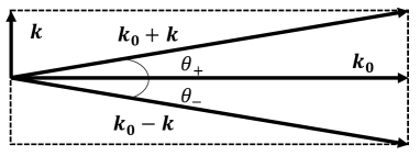
Figure 1: Wavevector diagram for the FI.

We now estimate the maximum growth rate of the FI. For the FI, we can safely assume $\mbox{\boldmath$k$}\cdot\mbox{\boldmath$k_{0}$}\sim 0$ and $\cos\theta_{\pm}\sim 1$. For $|\omega|\ll ck$, Equation 19 reduces to

$$\left(\omega^{2}-c_{s}^{2}k^{2}\right)\left(\omega^{2}-\frac{c^{4}k^{4}}{4\omega_{0}^{2}}\right)=\frac{a_{0}^{2}\omega_{pe}^{2}c^{4}k^{4}}{4\omega_{0}^{2}}.$$ (27)

Substituting $\omega=i\Gamma$, where $\Gamma\ll c_{s}k$, into Equation 27, we obtain

$$\Gamma^{2}+\frac{c^{4}k^{4}}{4\omega_{0}^{2}}=\frac{a_{0}^{2}\omega_{pe}^{2}c^{2}k^{2}}{4\omega_{0}^{2}\beta_{s}^{2}}.$$ (28)

The condition $\Gamma\ll c_{s}k$ is generally referred to as the weak coupling regime (e.g., Drake et al., 1974; Forslund et al., 1975; Cohen & Max, 1979; Kruer, 1988). We can find the maximum growth rate and corresponding wavevector,

$$\Gamma_{max}=\frac{a_{0}^{2}\omega_{pe}^{2}}{4\beta_{s}^{2}\omega_{0}}\ {\rm(weak\ coupling)},$$ (29)

$$k_{y}=\frac{a_{0}\omega_{pe}}{\sqrt{2}c\beta_{s}}\ {\rm(weak\ coupling)}.$$ (30)

The validity condition $\Gamma\ll c_{s}k$ is

$$\beta_{s}\gg\sqrt{a_{0}\frac{\omega_{pe}}{\omega_{0}}}\ {\rm(weak\ coupling)}.$$ (31)

For $\Gamma\gg c_{s}k$, which is the so-called strong coupling regime, Equation 27 reduces to

$$\Gamma^{4}+\frac{c^{4}k^{4}}{4\omega_{0}^{2}}\Gamma^{2}=\frac{a_{0}^{2}\omega_{pe}^{2}c^{4}k^{4}}{4\omega_{0}^{2}}.$$ (32)

The growth rate increases with $k$ and the asymptotic solution is written as

$$\Gamma_{max}=a_{0}\omega_{pe}\ {\rm(strong\ coupling)}.$$ (33)

$\Gamma$ is then expanded for large $k$,

$$\Gamma=\left(1-\frac{4a_{0}^{2}\omega_{0}^{2}\omega_{pe}^{2}}{c^{4}k^{4}}\right)\Gamma_{max}.$$ (34)

Thus $\Gamma$ asymptotically approaches the maximum for

$$k\gg\frac{\sqrt{a_{0}\omega_{0}\omega_{pe}}}{c}.$$ (35)

We have neglected factors of order of unity. The validity condition is

$$\frac{\sqrt{a_{0}\omega_{0}\omega_{pe}}}{c}\ll k_{y}\ll\frac{a_{0}\omega_{pe}}{c\beta_{s}}\ {\rm(strong\ coupling)},$$ (36)

$$\beta_{s}\ll\sqrt{a_{0}\frac{\omega_{pe}}{\omega_{0}}}\ {\rm(strong\ coupling)}.$$ (37)

This condition and maximum growth rate show that the e-folding time of the FI $\tau_{grow}\sim 1/\Gamma_{max}\sim 1/a_{0}\omega_{pe}$ is much shorter than the sound crossing time of the density filaments $\tau_{cross}\sim 1/c_{s}k_{y}\gg 1/a_{0}\omega_{pe}$ for the strong coupling regime. On the other hand, $\tau_{cross}/\tau_{grow}\sim a_{0}\omega_{pe}/\beta_{s}^{2}\omega_{0}\ll 1$ is satisfied for the weak coupling regime. This difference affects the heating physics during the linear and nonlinear evolution of the FI (see Section 3.3).

2.2 Fully Kinetic Formulation

We here assume an unmagnetized pair plasma governed by the Vlasov equation,

$$\frac{\partial f_{j}}{\partial t}+\mbox{\boldmath$v_{j}$}\cdot\frac{\partial f_{j}}{\partial\mbox{\boldmath$x$}}+\frac{q_{j}}{m_{j}c}\left[-\frac{\partial\mbox{\boldmath$A$}}{\partial t}+\mbox{\boldmath$v_{j}$}\times(\mbox{\boldmath$\nabla$}\times\mbox{\boldmath$A$})\right]\cdot\frac{\partial f_{j}}{\partial\mbox{\boldmath$u$}}=0,$$ (38)

$$\mbox{\boldmath$J$}=\sum_{j}q_{j}\int\mbox{\boldmath$v$}f_{j}{\rm d}\mbox{\boldmath$u$},$$ (39)

where $u=\gamma\mbox{\boldmath$v$}$ is the particle four velocity. Let us assume that the zeroth-order distribution function $f_{0j}$ satisfies

$$\int f_{0j}{\rm d}\mbox{\boldmath$u$}=n_{0}\left(1-\frac{1}{4}a_{0}^{2}\cos 2\phi_{0}\right),$$ (40)

which is motivated by the fluid approximation in Equation 12. $f_{0j}$ is then written as

$$f_{0j}=n_{0}\left(1-\frac{1}{4}a_{0}^{2}\cos 2\phi_{0}\right)F_{0}(\mbox{\boldmath$u_{j\perp}$})\delta\left(\mbox{\boldmath$u_{j\parallel}$}+\frac{q_{j}\mbox{\boldmath$A$}}{m_{j}}\right),$$ (41)

where $u_{j\parallel}$ and $u_{j\perp}$ are the four velocity components of parallel and perpendicular to the vector potential $A$, respectively. The $\delta$ is the Dirac delta function and this term comes from the conservation of the canonical momentum. For $a_{0}\ll 1$, $F_{0}$ is given by the non-relativistic 1D Maxwellian distribution,

$$F_{0}=\frac{1}{\sqrt{2\pi}v_{th0}}\exp\left[-\frac{v_{x}^{2}}{2v_{th0}^{2}}\right],$$ (42)

where $v_{th0}=\sqrt{k_{B}T_{e}/m_{e}}$ is the thermal velocity and the electron temperature $T_{e}$ is equal to the positron one $T_{p}$. Substituting $A_{0}$ and $f_{0j}$ into the Vlasov and wave equations, we obtain the dispersion relation

$$\omega_{0}^{2}-c^{2}k_{0}^{2}-2\omega_{pe}^{2}\left(1-\frac{1}{4}a_{0}^{2}\right)=0,$$ (43)

which is identical to the fluid approximation. Considering only the lowest-order coupling, which is valid for $a_{0}\ll 1$, the perturbed quantities can be expressed as

$$\mbox{\boldmath$A$}=\mbox{\boldmath$A_{0}$}+\mbox{\boldmath$\delta A_{+}$}e^{i\phi_{+}}+\mbox{\boldmath$\delta A_{-}$}e^{i\phi_{-}}+c.c.,$$ (44)

$$f_{j}=n_{0}\left(1-\frac{1}{4}a_{0}^{2}\cos 2\phi_{0}\right)(F_{0}+\delta Fe^{i\phi})\delta\left(\mbox{\boldmath$u_{j\parallel}$}+\frac{q_{j}\mbox{\boldmath$A$}}{m_{j}}\right)+c.c.,$$ (45)

where $\delta F$ is independent of $u_{j\parallel}$. Linearizing the basic equations, we finally obtain the fully kinetic dispersion relation,

$$\frac{1}{2}a_{0}^{2}\omega_{pe}^{2}(Q_{kin}-1)\left(\frac{\cos^{2}\theta_{+}}{D_{+}}+\frac{\cos^{2}\theta_{-}}{D_{-}}\right)=1,$$ (46)

where

$$Q_{kin}=\frac{c^{2}}{2v_{th0}^{2}}\frac{{\rm d}Z}{{\rm d}\zeta},$$ (47)

$$\zeta=\frac{\omega}{\sqrt{2}v_{th0}k}.$$ (48)

$Z(\zeta)$ is the plasma dispersion function given by

$$Z(\zeta)=\frac{1}{\sqrt{\pi}}\int_{-\infty}^{\infty}\frac{e^{-z^{2}}}{z-\zeta}{\rm d}z,$$ (49)

$$\frac{{\rm d}Z}{{\rm d}\zeta}=-2(1+\zeta Z).$$ (50)

The difference from the fluid approximation is that the sound wave dispersion relation in Equation 19 is replaced by the kinetic one.

We numerically derive the linear growth rate of the FI and show it in Figure 2 for $(a_{0},\omega_{0}/\omega_{pe},\beta_{th0})=(0.3,30,0.01)$ (left) and $(0.3,30,0.1)$ (right). Our simulations are performed for these two cases. The black solid lines in Figure 2 indicate the kinetic growth rates. We also show the fluid ones with the adiabatic index $\gamma_{ad}=1$ (isothermal) and $\gamma_{ad}=3$ (1D gas) in red and blue dashed lines, respectively. The left panel refers to the strong coupling regime $|\omega|\gg c_{s}k$. Since the results of fluid and kinetic calculations are comparable as further discussed below, we can safely use the analytical estimates from the fluid approximation and Equation 33 and 36 give, for the strong coupling regime,

$$\frac{\Gamma_{max}}{\omega_{0}}\sim 1.0\times 10^{-2},$$ (51)

$$0.1\ll\frac{k_{y}}{k_{0}}\ll 1.$$ (52)

In contrast, for the weak coupling regime $|\omega|\ll c_{s}k$ in the right panel, the maximum growth rate and the corresponding wavevector are estimated from Equation 29 and 30,

$$\frac{\Gamma_{max}}{\omega_{0}}\sim 2.5\times 10^{-3},$$ (53)

$$\frac{k_{y}}{k_{0}}\sim 0.07.$$ (54)

Here we have assumed $\beta_{s}\sim\beta_{th0}$. These analytical estimates are roughly consistent with the numerical results.

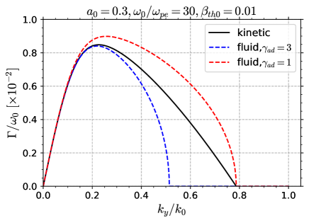
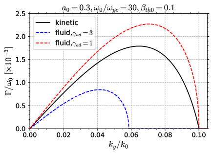
Figure 2: Linear growth rate of the FI for the strong (left) and weak (right) coupling cases.

We now expand why the fluid and kinetic calculations give comparable results. This is not surprising because the density fluctuation is a non-propagating mode and the FI is almost unaffected by the Landau damping as already discussed by Cohen & Max (1979). The derivative of the plasma dispersion function is expressed by the expansion (see, e.g., Fried & Conte, 1961) for $|\zeta|\gg 1$ (i.e., strong coupling regime $|\omega|\gg c_{s}k$),

$$\frac{{\rm d}Z}{{\rm d}\zeta}=\frac{1}{\zeta^{2}}+\frac{3}{2}\frac{1}{\zeta^{4}}+\frac{15}{4}\frac{1}{\zeta^{6}}+\cdots,$$ (55)

and for $|\zeta|\ll 1$,

$$\frac{{\rm d}Z}{{\rm d}\zeta}=-2\sqrt{\pi}i\zeta e^{-\zeta^{2}}-2+4\zeta^{2}-\frac{8}{3}\zeta^{4}+\cdots.$$ (56)

Here we have used ${\rm Im}(\zeta)>0$. $Q_{kin}$ is thus approximately expressed as for the strong coupling regime $|\omega|\gg c_{s}k$,

$$Q_{kin}\simeq\frac{c^{2}k^{2}}{\omega^{2}}\left(1+\frac{3v_{th0}^{2}k^{2}}{\omega^{2}}\right).$$ (57)

and for the weak coupling regime $|\omega|\ll c_{s}k$,

$$Q_{kin}\simeq-\frac{c^{2}}{v_{th0}^{2}}.$$ (58)

$Q_{fluid}$ is expressed as for $|\omega|\gg c_{s}k$,

$$Q_{fluid}\simeq\frac{c^{2}k^{2}}{\omega^{2}}\left(1+\frac{c_{s}^{2}k^{2}}{\omega^{2}}\right).$$ (59)

and for $|\omega|\ll c_{s}k$,

$$Q_{fluid}\simeq-\frac{c^{2}}{c_{s}^{2}}.$$ (60)

If we assume the adiabatic index $\gamma_{ad}=3$ for $|\omega|\gg c_{s}k$ and $\gamma_{ad}=1$ for $|\omega|\ll c_{s}k$, $Q_{kin}$ is identical to $Q_{fluid}$. Therefore, the fluid approximation for the FI is reasonable.

On the other hand, the effect of the Landau damping is not negligible for the SBS because the SBS induces sound-like waves which are heavily damped unless a strong temperature difference between electrons and positrons is induced. The fluid approximation for the SBS is then valid only for the strong coupling regime (see Appendix A).

3 Numerical Simulation

3.1 Setup

We use a fully kinetic particle-in-cell (PIC) code (Matsumoto et al., 2015, 2017), which employs an implicit Maxwell solver without any digital filters (Ikeya & Matsumoto, 2015), a charge conservation scheme for the electric current deposition (Esirkepov, 2001), and a second-order shape function for computational macroparticles. We consider a rectangular simulation box in $x$-$y$ plane and the boundary condition in all directions is periodic for both the fields and the particles. All three components of fields and velocities are tracked in our simulations. The initial condition is based on Ghosh et al. (2022). The plane monochromatic pump wave is initially introduced,

$$E_{0} =(0,E_{0}\cos{k_{0}x},0),$$ (61)

$$B_{0} =\left(0,0,\frac{ck_{0}}{\omega_{0}}E_{0}\cos{k_{0}x}\right).$$ (62)

We also study the case of a pump wave vector potential perpendicular to simulation plane (see Appendix B). This pump wave propagates through homogeneous, unmagnetized pair plasmas with a Maxwellian distribution. We calculate the initial thermal spread $\beta_{th0}$ in the proper frame. The initial bulk four velocity satisfies

$$\bar{u}_{0jx} =\frac{1}{2}ca_{0}^{2}\sin^{2}{k_{0}x},$$ (63)

$$\bar{u}_{0jy} =\pm ca_{0}\sin{k_{0}x},$$ (64)

$$\bar{u}_{0jz} =0,$$ (65)

where the positive (negative) sign corresponds to the electron (positron). The SBS generally grows faster than the FI for monochromatic pump waves (Ghosh et al., 2022). The simulation domain in the $x$ direction is just one wavelength of the pump wave $L_{x}=\lambda_{0}$, where $\lambda_{0}$ is the wavelength of the pump wave. Since the backward SBS is most unstable and the wavenumber of the back-scattered wave can be estimated as $\mbox{\boldmath$k_{s}$}=\mbox{\boldmath$k_{0}$}-\mbox{\boldmath$k$}\simeq-(1-2\beta_{s})k_{0}\mbox{\boldmath$\hat{x}$}$ (e.g., Kruer, 1988), the SBS can be suppressed by a small box as already discussed by Ghosh et al. (2022). This is the case for the weak coupling case, however, the SBS grows into an substantial amplitude for the strong coupling case (see Appendix A). The simulation domain in the $y$ direction is $L_{y}=120\lambda_{0}=8\pi c/\omega_{pe}$ to follow the filament mergers. The grid size and time step are respectively set as $\Delta x/\lambda_{0}=0.005$ and $\omega_{0}\Delta t=0.0314$. The number of particles per cell per species is $n_{0}\Delta x^{2}=32$. Tests of numerical convergence are shown in Appendix C.

We fix the pump wave frequency $\omega_{0}/\omega_{pe}=30$ and the wave strength parameter $a_{0}=0.3$ throughout this study. We carry out our simulations for strong and weak coupling cases: $\beta_{th0}=0.01$ and $0.1$, which satisfy the condition 1.

3.2 Simulation Results

Figure 3 shows the time evolution of the transverse electron density fluctuations $\delta n_{e}(y)=\sqrt{\langle n_{e}-n_{0}\rangle_{x}^{2}}$ for $\beta_{th0}=0.01$ (left) and $0.1$ (right), where $\langle\rangle_{x}$ indicates the physical quantities averaged over the $x$ (pump wave propagation) direction. We compute the power spectrum of $\delta n_{e}(y)$ and then take its square root for Figure 3. Note that the horizontal axis range in units of $\omega_{0}$ is different. The most unstable modes are shown in blue. The total of all modes (i.e., the spectrum-integrated signal), which is shown in red, is strongly dominated by the most unstable mode at the linear phase $\Gamma_{max}t\lesssim 10$, where $\Gamma_{max}$ is the maximum growth rate numerically determined from the linear theory (Equation 46 for $k_{x}=0$). In both cases, the density filaments exponentially grow until $\Gamma_{max}t\sim 10$ and then they get saturated. The maximum growth rates $\Gamma_{max}$ determined from linear theory (black dashed lines) give a good agreement with our simulation results. In the nonlinear phase $\Gamma_{max}t\gtrsim 10$, the time evolution of the most unstable mode gradually deviates from the total because the filaments begin to merge and the wavenumber of the mode with the highest power gradually decreases, as further discussed below.

The time history of the electron thermal velocity $\langle\beta_{th}\rangle$ averaged over the whole simulation domain is shown in green (axis on the right of each panel). The thermal velocity is calculated in the fluid rest frame for each species. Note that the vertical axis for $\langle\beta_{th}\rangle$ is in linear scale. For the strong coupling regime (left in Figure 3), $\langle\beta_{th}\rangle$ increases for $\omega_{0}t\lesssim 200$ due to the SBS (see Appendix A). However, most of the heating happens during the nonlinear evolution of the FI and we thus think that the SBS has little impact on the FI growth. The increase of $\langle\beta_{th}\rangle$ at early times is not seen for the weak coupling regime (right in Figure 3), demonstrating that the SBS is well-suppressed for $\beta_{th0}=0.1$.

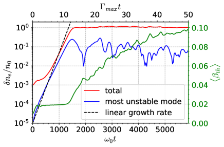
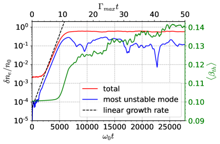
Figure 3: Time evolution of the amplitude of the transverse electron density fluctuations $\delta n_{e}$ for $\beta_{th0}=0.01$ (left) and $0.1$ (right). The most unstable modes (blue) and total of all Fourier modes (red) are shown. The black dashed lines represent $\propto e^{\Gamma_{max}t}$, where $\Gamma_{max}$ is the maximum growth rate determined from linear theory (Equation 46 for $k_{x}=0$). The time history of the box-averaged thermal velocity $\langle\beta_{th}\rangle$ is shown in green (axis on the right of each panel).

Figure 4 shows the temporal evolution of the $x$-averaged electron density $\langle n_{e}\rangle_{x}$ (top panels) and $x$ component of the Poynting flux $\langle S_{x}\rangle_{x}$ (bottom panels) for $\beta_{th0}=0.01$ (left column) and $0.1$ (right column), where $\langle S_{x}\rangle_{x}$ is normalized by the initial mean flux $S_{0}=E_{0}^{2}/8\pi$. In the linear phase $\Gamma_{max}t\lesssim 10$, the amplitude of the density filaments for $\beta_{th0}=0.01$ is larger than for $\beta_{th0}=0.1$, because colder plasmas are more easily compressed by the wave ponderomotive force due to their weaker pressure gradients. In the final state of our simulations, the density amplitudes are comparable between the two cases, because the plasma gets heated during the nonlinear evolution of the FI and the temperatures become comparable in the two cases, as shown with the grey lines in Figure 3 and further discussed in Section 3.3. The density filaments gradually merge for $\Gamma_{max}t\gtrsim 10$ and the filament merging continues until the wavelength of the filament reaches $\sim 2\pi c/\omega_{pe}$, i.e., comparable to the electron skin depth. We discuss the saturation of the filament merging in Section 3.3. The wave Poynting flux peaks in the lower density regions, i.e., the wave power accumulates in the density cavities. The electromagnetic waves then propagate between the density filaments as in a waveguide.

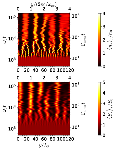
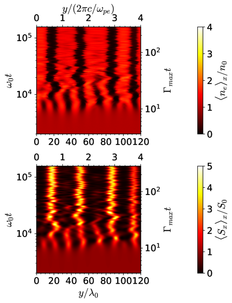
Figure 4: Time evolution of the $x$-averaged electron density (top panels) and $x$ component of the $x$-averaged Poynting flux (bottom panels) for $\beta_{th0}=0.01$ (left column) and $0.1$ (right column).

Figure 5 shows the time evolution of the power spectra of the $x$-averaged electron density fluctuations for $\beta_{th0}=0.01$ (left) and $0.1$ (right). The blue lines correspond to the wavenumber of the theoretical fastest-growing modes: $k_{y}/k_{0}\sim 0.2$ for $\beta_{th0}=0.01$ and $k_{y}/k_{0}\sim 0.07$ for $\beta_{th0}=0.1$ in Figure 2. The observed peaks at the linear stage $\Gamma_{max}t\lesssim 10$ are consistent with the theoretical estimates. The most unstable wavenumber gradually decreases down to $\sim\omega_{pe}/c$.

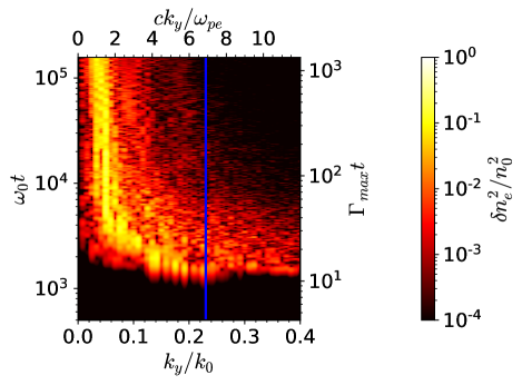
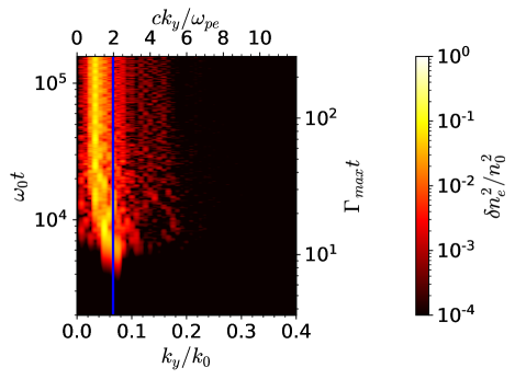
Figure 5: Time evolution of the power spectra of the $x$-averaged electron density fluctuations for $\beta_{th0}=0.01$ (left) and $0.1$ (right). The blue lines indicate the theoretical fastest-growing modes.

3.3 Saturation Mechanism of Filament Merging

The FI saturates when force balance between the pressure gradient and ponderomotive force is achieved (Kaw et al., 1973; Sobacchi et al., 2023). The ponderomotive force exerted by the electromagnetic wave expels particles from the region of high intensity. The pressure gradient is gradually amplified by the compression and it finally balances the ponderomotive force. Figure 6 shows snapshots of the $x$-averaged ponderomotive force (blue) and plasma pressure (red) normalized by $eE_{0}$ at the final state of our simulations $\omega_{0}t=157254$ for $\beta_{th0}=0.01$ (left) and $0.1$ (right). The pressure gradient $\nabla p_{e}$ is the $y$ derivative of the $yy$ component of the pressure tensor and averaged over the $x$ direction. The ponderomotive force is by definition the sum of the advection and nonlinear Lorentz force averaged over the wave period. We determine the $y$ component of the ponderomotive force $F_{pond}$ for electrons from the snapshots averaged over the $x$ direction (i.e., one wavelength of the pump wave),

$$F_{pond}=\left\langle-(\mbox{\boldmath$v_{e}$}\cdot\mbox{\boldmath$\nabla$})v_{ey}-\frac{e}{m_{e}c}(v_{ez}B_{x}-v_{ex}B_{z})\right\rangle_{x}$$ (66)

The green lines indicate the $x$-averaged electron density. The electromagnetic waves escape from the higher density region as shown in the bottom panels of Figure 4, and thus the ponderomotive force vanishes there. The force balance between the pressure gradient and ponderomotive force is clearly achieved across the whole transverse direction.

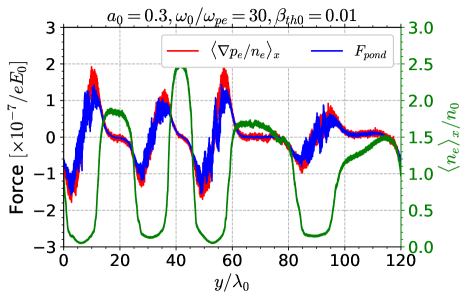
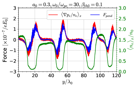
Figure 6: Snapshots of the ponderomotive force (blue) and pressure gradient (red) at the final state $\omega_{0}t=157254$ for $\beta_{th0}=0.01$ (left) and $0.1$ (right). The green lines indicate the $x$-averaged electron density.

Sobacchi et al. (2023) discussed the saturation mechanism of the FI based on the assumption that the adiabatically-compressed density filaments are supported by the ponderomotive force in the steady state. They pointed out that non-adiabatic heating can be important for the strong coupling regime and it can raise the plasma temperature because the force balance between the ponderomotive force and the pressure gradient does not have time to be established for $\tau_{grow}\ll\tau_{cross}$, where $\tau_{grow}$ is the e-folding time of the FI and $\tau_{cross}$ is the sound crossing time of the density filaments. To investigate the effect of the non-adiabatic heating, we measure the thermal velocity in our simulations. Figure 7 shows the electron thermal velocity (black) at the final state of our simulations $\omega_{0}t=157254$, which is the same time as Figure 6, for $\beta_{th0}=0.01$ (left) and $0.1$ (right). The green lines indicate the $x$-averaged electron density. If only the adiabatic compression contributes to the plasma heating, the thermal velocity satisfies

$$\frac{\beta_{th}^{2}}{n_{e}^{\gamma_{ad}-1}}=const.,$$ (67)

The adiabatic thermal velocity is determined from the measured density profile adopting a choice of $\gamma_{ad}=3$ and shown in blue. For the weak coupling case $\beta_{th0}=0.1$ (right in Figure 7), the thermal velocity in the higher density region is well-explained by the adiabatic heating. The non-adiabatic heating operates in the density cavity and is associated with the filament mergers. For the strong coupling regime $\beta_{th0}=0.01$ (left in Figure 7), the thermal velocity at the final time is much larger than the adiabatic heating, indicating that the non-adiabatic heating is dominant.

The non-adiabatic heating may saturate when the equipartition between the ponderomotive potential and total (electron + positron) thermal energy is achieved. Since the initial ponderomotive potential is $m_{e}c^{2}a_{0}^{2}/4$, the equipartition thermal energy is $m_{e}c^{2}a_{0}^{2}/8$ and the thermal velocity is thus

$$\beta_{th}\sim\frac{a_{0}}{2\sqrt{2}},$$ (68)

which is shown in red in Figure 7. This estimate is roughly consistent with the measured thermal velocity at the final time. The filament merging continues until the wavelength of the filament reaches $\sim 2\pi c/\omega_{pe}$ as already shown. The saturation wavelength may be explained by an argument relying as well on the saturation thermal velocity. If the linear analysis is still valid at the saturation stage, Equation 30 for $\beta_{s}\sim a_{0}/2\sqrt{2}$ reduces to $k_{y}\sim\omega_{pe}/c$ in the weak coupling case. In the strong coupling case, Equation 36 reduces to

$$\frac{\omega_{pe}}{c}<k_{y}<\frac{2\sqrt{2}\omega_{pe}}{c},$$ (69)

where $\omega_{0}\gg\omega_{pe}/a_{0}$ is applied. The wavenumber of the most unstable mode may gradually approach the inverse skin depth due to the non-adiabatic heating.

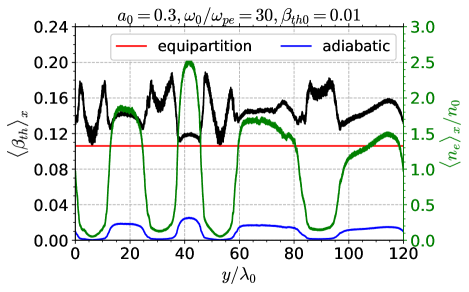
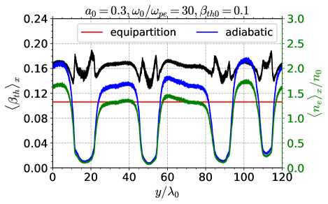
Figure 7: Snapshots of the electron thermal velocity (black) at the final state $\omega_{0}t=157254$ for $\beta_{th0}=0.01$ (left) and $0.1$ (right). The $x$-averaged electron density is shown in green. The thermal velocity determined from the adiabatic relation $\beta_{th}^{2}/n_{e}^{2}=const.$ is shown in blue. The red lines indicate the thermal velocity for the energy equipartition.

4 Summary and Discussion

We study the nonlinear evolution of the filamentation instability (FI) of strong electromagnetic waves in pair plasmas using 2D PIC simulations. Our simulations show that the FI generates transverse density filaments and that the electromagnetic waves propagate in near vacuum between the density filaments, as in a waveguide. We find that the density filaments merge until the filament wavelength reaches the electron skin depth. The filament merging ceases when force balance between the ponderomotive force and the pressure gradient is established. Non-adiabatic heating operates during the evolution of the FI and can be important especially in the strong coupling regime, i.e. when the e-folding time of the FI is shorter than the sound travel time across the filaments. Non-adiabatic heating may saturate when equipartition between the ponderomotive potential and the plasma thermal energy is achieved.

We now discuss the implications of our results for Fast Radio Bursts (FRBs). The FRB propagation has four important time scales: (i) the time scale on which the FI exponentially grows, $\tau_{FI}$, (ii) the filament merging time scale $\tau_{merge}$, (iii) the pulse duration time $\tau_{pulse}$, and (iv) the expansion time of the wave front $\tau_{exp}$. We estimate $\tau_{merge}$ from our simulations in the strong coupling regime, as appropriate for FRBs (Sobacchi et al., 2023). Figure 8 shows the time evolution of the peak wavenumber of the power spectrum (taken from the left panel of Figure 5). The blue solid line indicates the fastest-growing modes from linear theory, which agrees with the simulation results in the linear phase $t\lesssim\tau_{FI}\sim 10/\Gamma_{max}$. Since the peak wavenumber exponentially decreases until $\Gamma_{max}t\sim 40$, we define the merging time as $\tau_{merge}\sim 4\tau_{FI}\sim 40/\Gamma_{max}$. Evaluating $\Gamma_{max}$ from linear theory, the merging time $\tau_{merge}$ in the rest frame of the magnetar wind can then be estimated as

$$\tau_{merge}\sim 80\,{\rm ms}\left(\frac{L}{10^{42}{\rm\;erg\ s^{-1}}}\right)^{-\frac{1}{2}}\left(\frac{\dot{N}}{10^{39}{\rm\;s^{-1}}}\right)^{-\frac{1}{2}}\\ \times\left(\frac{\gamma_{w}}{10^{2}}\right)^{\frac{1}{2}}\left(\frac{\nu_{obs}}{1{\rm\;GHz}}\right)\left(\frac{R}{10^{14}{\rm\;cm}}\right)^{2},$$ (70)

where $L$ is the observed radio luminosity, $\dot{N}$ is the particle outflow rate, $\gamma_{w}$ is the wind bulk Lorentz factor, $\nu_{obs}$ is the obserbed radio frequency, and $R$ is the distance from the source (Beloborodov, 2020; Sobacchi et al., 2023). The time duration of the radio pulse in the wind rest frame $\tau_{pulse}$ is

$$\tau_{pulse}=2\gamma_{w}\tau_{obs}\sim 200\,{\rm ms}\left(\frac{\gamma_{w}}{10^{2}}\right)\left(\frac{\tau_{obs}}{1{\rm\;ms}}\right),$$ (71)

where $\tau_{obs}$ is the observed pulse duration. The expansion time of the wave front in the wind frame is

$$\tau_{exp}=\frac{R}{2\gamma_{w}c}\sim 20\,{\rm s}\left(\frac{R}{10^{14}{\rm\;cm}}\right)\left(\frac{\gamma_{w}}{10^{2}}\right)^{-1}.$$ (72)

Since $\tau_{FI}\lesssim\tau_{merge}\lesssim\tau_{pulse}\ll\tau_{exp}$, the radio wave is filamented, and the filaments merge before the radio pulse can propagate through the unperturbed plasma ahead of the wave front.

The merging time may get longer for the realistic case in which the peak wavenumber in the linear stage is $\gg\omega_{pe}/c$, a case we cannot achieve due to computational limitations. Then the filamentation instability may develop in the regime where the merging time is longer than the duration of the radio pulse, i.e. $\tau_{FI}\lesssim\tau_{pulse}\lesssim\tau_{merge}\ll\tau_{exp}$. In this regime the evolution of the filaments on the time scale $\tau_{merge}$ is unclear. Our simulations employ a periodic boundary condition in the wave propagation direction, so the radio pulse continuously interacts with density filaments. In contrast, for realistic FRB conditions the density filaments are non-propagating and stop interacting with the radio pulse after the time scale $\tau_{pulse}$. Then the pulse should propagate through an unperturbed plasma ahead of the wave front. We will study the effect of more realistic boundary conditions—including a self-consistent description of wave propagation—in a future publication.

We assumed that the initial velocity distribution is isotropic in this study. When plasmas are highly magnetized, which is the case for the magnetar wind, a temperature anisotropy is generally expected. Sobacchi et al. (2022) discussed the effect of the ambient magnetic field and demonstrated that the FI is independent on the thermal velocity in the direction perpendicular to the ambient magnetic field because the ponderomotive force preferentially pushes particles along the parallel direction. Therefore, we expect that the FI should be primarily affected by the parallel temperature for the anisotropic velocity distribution.

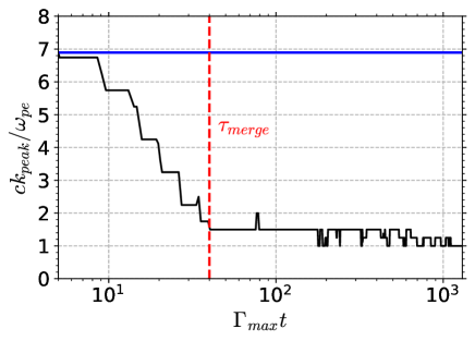
Figure 8: Time evolution of the peak wavenumber for the strong coupling regime $\beta_{th0}=0.01$ in the left panel of Figure 5. The blue solid line indicates the fastest-growing mode from the linear theory.

Our results are valid for the weak pump wave condition $a_{0}\ll 1$, in which the particle oscillation velocities in the wave fields are much smaller than the speed of light. The radio pulses are much stronger near the FRB progenitors and $a_{0}\gtrsim 1$ can be satisfied for $R\lesssim 10^{13}{\rm cm}$ (Luan & Goldreich, 2014; Beloborodov, 2020). In this relativistic regime, higher order couplings $(\omega_{n},\mbox{\boldmath$k_{n}$})=(\omega+n\omega_{0},\mbox{\boldmath$k$}+n\mbox{\boldmath$k_{0}$})$, where $n=\pm 2,\pm 3,\pm 4,...$ is an integer, are no longer negligible. We will explore the relativistic regime $a_{0}\gtrsim 1$ in a future publication.

DATA AVAILABILITY

The simulation code is available on request.

Appendix A Stimulated Brillouin Scattering

The maximum growth rate of the SBS can be derived from the same dispersion relation as the FI. $\cos\theta_{\pm}=-1$ is satisfied for the backward scattering and $D_{+}$ is non-resonant for the SBS. The dispersion relation 19 reduces to

$$(\omega^{2}-c_{s}^{2}k^{2})\left[\omega+\frac{c^{2}}{2\omega_{0}}(k-2k_{0})k\right]=-\frac{a_{0}^{2}\omega_{pe}^{2}c^{2}k^{2}}{4\omega_{0}}$$ (73)

Substituting $\omega=c_{s}k+i\Gamma$, where $\Gamma\ll c_{s}k$ for the weak coupling, we obtain

$$\Gamma^{2}-\frac{a_{0}^{2}\omega_{pe}^{2}c^{2}k}{8c_{s}\omega_{0}}-\frac{i\Gamma c^{2}}{2\omega_{0}}\left[k-2\left(k_{0}-\frac{c_{s}\omega_{0}}{c^{2}}\right)\right]k=0.$$ (74)

The maximum growth rate and corresponding wavevector are written as

$$\Gamma_{max}^{SBS}=\frac{a_{0}\omega_{pe}}{2\sqrt{\beta_{s}}},$$ (75)

$$k_{x}^{SBS}=2(1-\beta_{s})k_{0}.$$ (76)

The validity condition $\Gamma\ll c_{s}k$ now becomes

$$\beta_{s}\gg\left(a_{0}\frac{\omega_{pe}}{\omega_{0}}\right)^{\frac{2}{3}}.$$ (77)

Here we have neglected factors of order of unity. For the strong coupling $\Gamma\gg c_{s}k$, we obtain

$$\omega^{3}+\frac{c^{2}}{2\omega_{0}}(k-2k_{0})k\omega^{2}+\frac{a_{0}^{2}\omega_{pe}^{2}c^{2}k^{2}}{4\omega_{0}}=0$$ (78)

The growth rate takes its maximum at around $k=2k_{0}$ and we find

$$\omega=(a_{0}^{2}\omega_{pe}^{2}\omega_{0})^{\frac{1}{3}}e^{\frac{\pi i}{3}}.$$ (79)

We finally obtain

$$\Gamma_{max}^{SBS}=\frac{\sqrt{3}}{2}(a_{0}^{2}\omega_{pe}^{2}\omega_{0})^{\frac{1}{3}},$$ (80)

$$k_{x}^{SBS}=2k_{0},$$ (81)

and the validity condition is

$$\beta_{s}\ll\left(a_{0}\frac{\omega_{pe}}{\omega_{0}}\right)^{\frac{2}{3}}.$$ (82)

Our parameters $(a_{0},\omega_{0}/\omega_{pe},\beta_{th0})=(0.3,30,0.1)$ and $(0.3,30,0.01)$ satisfy the weak (Equation 77) and strong (Equation 82) coupling conditions for the SBS, respectively. We numerically derive the linear growth rate of the SBS and show it in Figure 9 for the strong (left) and weak (right) coupling cases. The SBS grows faster than the FI for both cases. For the weak coupling case, the kinetic growth rate is much smaller than the fluid one because the fluid growth rate is always overestimated due to the absence of Landau damping. The unstable wavevector is smaller than $2k_{0}$, indicating that the backscattered waves propagating the $-x$ direction are not resolved in our simulation box $L_{x}\times L_{y}=\lambda_{0}\times 120\lambda_{0}$, which helps to suppress the SBS as already discussed by Ghosh et al. (2022). In fact, for hot plasmas with $\beta_{th0}=0.1$, we find that the amplitude of the SBS-generated density fluctuations is vary small ($\delta n_{e}/n_{0}\sim 10^{-2}$), i.e., the SBS is suppressed.

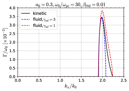
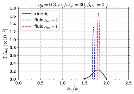
Figure 9: Linear growth rate of the SBS for strong (left) and weak (right) coupling cases.

In contrast, in the strong coupling case the unstable wavevector can exceed $2k_{0}$ and thus SBS operates even for our simulation setting. Figure 10 shows the snapshot of the electron density at $\omega_{0}t=629$ for $\beta_{th0}=0.01$ (left). The density fluctuation at the wavenumber $k_{x}\sim 2k_{0}$ is clearly seen, indicating that the SBS indeed operates for the strong coupling regime. The time evolution of the $y$-averaged electron density is shown in the right panel of Figure 10. The white dashed line represents fluctuations propagating with the sound speed $c_{s}$, where the adiabatic index $\gamma_{ad}=3$ is assumed, showing that the the density fluctuation at $k_{x}\sim 2k_{0}$ is propagating in the $+\mbox{\boldmath$x$}$ direction with the sound speed. Since the SBS is expected to generate the forward-propagating sound-like waves, this provides a clear proof of the SBS.

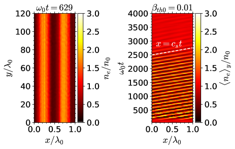
Figure 10: Left: snapshot of the electron density at $\omega_{0}t=629$. Right: time evolution of the $y$-averaged electron density. The white dashed line represents fluctuations propagating with the sound speed $c_{s}$.

Figure 11 shows the time evolution of Fourier components of the $y$-averaged density fluctuations for the strong coupling case $\beta_{th0}=0.01$. The black dashed lines are maximum growth rates $\Gamma_{max}$ of the SBS determined from the linear theory (Equation 46 for $k_{y}=0$), showing a good agreement with our simulation result. Based on the above analysis, we conclude that the longitudinal density fluctuation with $k_{x}\sim 2k_{0}$ originates from the SBS and that the SBS is not fully suppressed by our numerical setting for the strong coupling case.

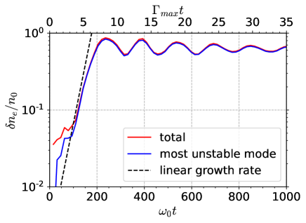
Figure 11: Time evolution of the SBS. The amplitude is calculated from the Fourier components of the $y$-averaged density fluctuations for $\beta_{th0}=0.01$. The most unstable modes (blue) and integral of all modes (red) are shown. The black dashed lines correspond to $\propto e^{\Gamma_{max}t}$, where $\Gamma_{max}$ is determined from the linear theory (Equation 46 for $k_{y}=0$).

Appendix B Out-of-plane Vector Potential

In the main text, we focus on the pump wave vector potential lying in the $y$ direction. One can choose the out-of-plane vector potential ($z$ direction in our coordinates) and the corresponding wave fields are

$$E_{0} =(0,0,E_{0}\cos{k_{0}x}),$$ (83)

$$B_{0} =\left(0,\frac{ck_{0}}{\omega_{0}}E_{0}\cos{k_{0}x},0\right).$$ (84)

In this case, $\mbox{\boldmath$A_{0}$}\parallel\mbox{\boldmath$\delta A_{\pm}$}$ (i.e, $\cos\theta_{\pm}=1$) is always satisfied regardless of the scattering direction, and thus side scattering ($\mbox{\boldmath$k_{0}$}\perp\mbox{\boldmath$k_{\pm}$}$) survives unlike in the in-plane configuration.

Figure 12 shows the time evolution of the $x$-averaged power spectrum for $\beta_{th0}=0.01$ in the out-of-plane configuration. The numerical parameters are identical to the in-plane configuration in the main text and only the direction of the initial vector potential changes. The clear peak can be no longer seen near the theoretical most unstable mode of the FI (the blue line in Figure 12). The filaments merge much earlier than the in-plane configuration. Furthermore, the mode with $k_{y}\sim 2k_{0}$ apparently grows faster than others, which is not observed the in-plane configuration. We think that the side-scattered wave plays the role of a pump wave and the peak at $k_{y}\sim 2k_{0}$ can be attributed to a secondary SBS of the side-scattered wave. In fact, the green line indicates the most unstable mode of the secondary SBS, showing a good agreement with the observed peak. Although the secondary SBS may induce the side-scattered wave again, the wavevector is almost identical to the pump wave and these waves cannot be distinguished. We here assumed that the wavenumber of the side-scattered wave, which plays a role for the pump wave of the secondary SBS, satisfies $\mbox{\boldmath$k_{s}$}\simeq\pm k_{0}\mbox{\boldmath$\hat{y}$}$. We confirmed this for $\beta_{th0}=0.1$ and the secondary SBS works for both strong and weak coupling cases. Note that our simulation setting can numerically suppress only the back-scattering which is the dominant mode of the SBS (Ghosh et al., 2022). The side-scattering survives even for the weak coupling regime in which the backward SBS is well-suppressed.

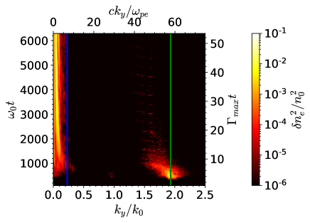
Figure 12: Time evolution of the power spectrum of the $x$-averaged electron density fluctuations for $\beta_{th0}=0.01$ with the out-of-plane vector potential. The blue and green lines correspond to the most unstable mode of the FI and SBS, respectively.

Figure 13 shows the time evolution of the $y$ component of the $x$-averaged Poynting flux $\langle S_{y}\rangle_{x}$ for $\beta_{th0}=0.01$, where $\langle S_{y}\rangle_{x}$ is normalized by the initial mean flux $S_{0}=E_{0}^{2}/8\pi$. The grid-like structures are clearly seen in addition to the transverse filamentary structures from the FI. The black dashed line represents the electromagnetic waves propagating in the $y$ direction, indicating that the grid-like structures originate from side-scattered waves traveling toward the $\pm y$ direction. It has been argued that side scattering for the out-of-plane vector potentials is numerically enhanced due to the periodic boundary condition in the $y$ direction (e.g., Cohen et al., 2005). We find that the side scattering preferentially works and dominates over the FI for the out-of-plane vector potentials.

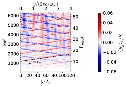
Figure 13: Time evolution of the $y$ component of the $x$-averaged Poynting flux for $\beta_{th0}=0.01$ with the out-of-plane vector potential. The black dashed line indicates the electromagnetic waves propagating in the $y$ direction.

Appendix C Numerical Convergence

Here, we demonstrate the convergence of the growth rate and saturation level with respect to the number of particles per cell per species $n_{0}\Delta x^{2}$.

Figure 14 shows the time evolution of the spectrum-integrated signal of $\delta n_{e}(y)$ for $\beta_{th0}=0.1$ for $n_{0}\Delta x^{2}=8$ (red), $16$ (green), $32$ (blue), and $64$ (purple). The black dashed line represents the fastest-growing mode from the linear theory. It is natural that the initial noise level should decrease as $n_{0}\Delta x^{2}$ increases. Both growth rate and saturation level converge for $n_{0}\Delta x^{2}\geq 32$. Based on this result, we choose $n_{0}\Delta x^{2}=32$ in the main text. In fact, the blue line shown in Figure 14 is the same as the red line in the right panel of Figure 3.

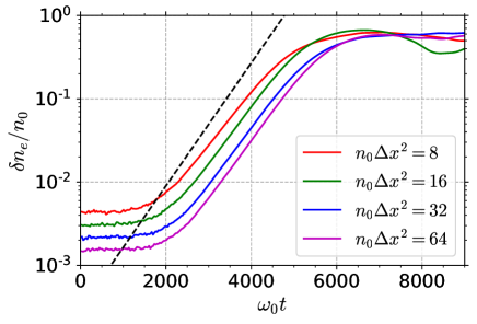
Figure 14: Numerical convergence with respect to the number of particles per cell per species for $\beta_{th0}=0.1$. The total of all Fourier modes of the transverse electron density fluctuations $\delta n_{e}$ is shown for $n_{0}\Delta x^{2}=8$ (red), $16$ (green), $32$ (blue), and $64$ (purple). The black dashed lines represent $\propto e^{\Gamma_{max}t}$.

References

- Andersen et al. (2020) Andersen B. C., et al., 2020, Nature, 587, 54
- Babul & Sironi (2020) Babul A.-N., Sironi L., 2020, MNRAS, 499, 2884
- Beloborodov (2017) Beloborodov A. M., 2017, ApJ, 843, L26
- Beloborodov (2020) Beloborodov A. M., 2020, ApJ, 896, 142
- Bochenek et al. (2020) Bochenek C. D., Ravi V., Belov K. V., Hallinan G., Kocz J., Kulkarni S. R., McKenna D. L., 2020, Nature, 587, 59
- Cohen & Max (1979) Cohen B. I., Max C. E., 1979, Phys. Fluids, 22, 1115
- Cohen et al. (2005) Cohen B. I., Divol L., Langdon A. B., Williams E. A., 2005, Phys. Plasmas, 12, 1
- Day et al. (2020) Day C. K., et al., 2020, MNRAS, 497, 3335
- Deutsch et al. (1996) Deutsch C., Furukawa H., Mima K., Murakami M., Nishihara K., 1996, Phys. Rev. Lett., 77, 2483
- Drake et al. (1974) Drake J. F., Kaw P. K., Lee Y. C., Schmid G., Liu C. S., Rosenbluth M. N., 1974, Phys. Fluids, 14, 778
- Edwards et al. (2016) Edwards M. R., Fisch N. J., Mikhailova J. M., 2016, Phys. Rev. Lett., 116, 015004
- Esirkepov (2001) Esirkepov T., 2001, Comput. Phys. Commun., 135, 144
- Forslund et al. (1975) Forslund D. W., Kindel J. M., Lindman E. L., 1975, Phys. Fluids, 18, 1002
- Fried & Conte (1961) Fried B. D., Conte S. D., 1961, The Plasma Dispersion Function: The Hilbert Transform of the Gaussian. Academic Press, New York
- Ghosh et al. (2022) Ghosh A., Kagan D., Keshet U., Lyubarsky Y., 2022, ApJ, 930, 106
- Ikeya & Matsumoto (2015) Ikeya N., Matsumoto Y., 2015, PASJ, 67, 64
- Iwamoto et al. (2017) Iwamoto M., Amano T., Hoshino M., Matsumoto Y., 2017, ApJ, 840, 52
- Iwamoto et al. (2022) Iwamoto M., Amano T., Matsumoto Y., Matsukiyo S., Hoshino M., 2022, ApJ, 924, 108
- Kaw & Dawson (1970) Kaw P., Dawson J., 1970, Phys. Fluids, 13, 472
- Kaw et al. (1973) Kaw P. K., Schmid G., Wilcox T., 1973, Phys. Fluids, 16, 1522
- Kruer (1988) Kruer W. L., 1988, The Physics of Laser Plasma Interactions. Addison-Wesley, Boston
- Lorimer et al. (2007) Lorimer D. R., Bailes M., McLaughlin M. A., Narkevic D. J., Crawford F., 2007, Science, 318, 777
- Luan & Goldreich (2014) Luan J., Goldreich P., 2014, ApJ, 785, L26
- Luo et al. (2020) Luo R., et al., 2020, Nature, 586, 693
- Lyubarsky (2014) Lyubarsky Y., 2014, MNRAS, 442, L9
- Lyubarsky (2021) Lyubarsky Y., 2021, Universe, 7, 56
- Margalit et al. (2020a) Margalit B., Metzger B. D., Sironi L., 2020a, MNRAS, 494, 4627
- Margalit et al. (2020b) Margalit B., Beniamini P., Sridhar N., Metzger B. D., 2020b, ApJ, 899, L27
- Matsukiyo & Hada (2003) Matsukiyo S., Hada T., 2003, Phys. Rev. E, 67, 046406
- Matsumoto et al. (2015) Matsumoto Y., Amano T., Kato T. N., Hoshino M., 2015, Sci, 347, 974
- Matsumoto et al. (2017) Matsumoto Y., Amano T., Kato T. N., Hoshino M., 2017, Phys. Rev. Lett., 119, 105101
- Max (1973a) Max C. E., 1973a, Phys. Fluids, 16, 1277
- Max (1973b) Max C. E., 1973b, Phys. Fluids, 16, 1480
- Max et al. (1974) Max C. E., Arons J., Langdon A. B., 1974, Phys. Rev. Lett., 33, 209
- Metzger et al. (2019) Metzger B. D., Margalit B., Sironi L., 2019, MNRAS, 485, 4091
- Michilli et al. (2018) Michilli D., et al., 2018, Nature, 553, 182
- Mima & Nishikawa (1975) Mima K., Nishikawa K., 1975, J. Phys. Soc. Jpn., 38, 1742
- Mima & Nishikawa (1984) Mima K., Nishikawa K., 1984, Basic Plasma Physics. North-Holland Publishing Company, Amsterdam
- Nimmo et al. (2021) Nimmo K., et al., 2021, Nature Astronomy, 5, 594
- Plotnikov & Sironi (2019) Plotnikov I., Sironi L., 2019, MNRAS, 485, 3816
- Plotnikov et al. (2018) Plotnikov I., Grassi A., Grech M., 2018, MNRAS, 477, 5238
- Schluck et al. (2017) Schluck F., Lehmann G., Spatschek K. H., 2017, Phys. Rev. E, 96, 053204
- Sironi et al. (2021) Sironi L., Plotnikov I., Nättilä J., Beloborodov A. M., 2021, Phys. Rev. Lett., 127, 035101
- Sluijter & Montgomery (1965) Sluijter F. W., Montgomery D., 1965, Phys. Fluids, 8, 551
- Sobacchi et al. (2021) Sobacchi E., Lyubarsky Y., Beloborodov A. M., Sironi L., 2021, MNRAS, 500, 272
- Sobacchi et al. (2022) Sobacchi E., Lyubarsky Y., Beloborodov A. M., Sironi L., 2022, MNRAS, 511, 4766
- Sobacchi et al. (2023) Sobacchi E., Lyubarsky Y., Beloborodov A. M., Sironi L., Iwamoto M., 2023, ApJ, 943, L21
- Tabak et al. (1994) Tabak M., et al., 1994, Phys. Plasmas, 1, 1626
- Tajima & Dawson (1979) Tajima T., Dawson J. M., 1979, Phys. Rev. Lett., 43, 267