Microscopic cut-off dependence of an entropic force in
interface propagation of stochastic order parameter dynamics
Yutaro Kado and Shin-ichi Sasa
Department of Physics, Kyoto University, Kyoto 606-8502, Japan
Abstract
The steady propagation of a -dimensional planer interface in -dimensional space is studied by analyzing mesoscopic non-conserved order parameter
dynamics with two local minima under the influence of thermal noise.
In this analysis,
an entropic force generating interface propagation is formulated using a perturbation method. It is found that the entropic force singularly
depends on an ultraviolet cut-off when . The theoretical calculation
is confirmed by numerical simulations with . The result
means that an experimental measurement of the entropic force provides
an estimation of the microscopic cut-off of the mesoscopic description.
Introduction.—
Macroscopic dynamics in nature are often described by deterministic equations. If a class of
phenomena is found to be described by a simple deterministic equation with a few parameters,
the phenomena can be studied by analyzing the universal equation. Fluid dynamics is a typical example of the success of such an approach [1]. However, there are cases in which simple deterministic equations cannot be found. For example, the macroscopic motion of locally conserved quantities in one or two dimensions cannot be described by a hydrodynamic equation with finite transportation coefficients [2]. Another example is the dynamical behavior near a critical point, where transport coefficients show a singular behavior [3, 4].
Even in such cases, a mesoscopic model with thermal noise can describe the macroscopic dynamical behavior. For example, fluctuating hydrodynamics can correctly describe the singular behavior of hydrodynamics in low dimensions [2]. The dynamical behavior near a critical point also can be described by the Ginzburg-Landau model with thermal noise [5]. Here, fluctuations modify the mean-field properties given by the mesoscopic free energy, which includes the transition type [6] as well as the critical exponents [5, 7]. These examples show that fluctuation effects at mesoscopic scales lead to the renormalization of model parameters and that the lack of a simple macroscopic equation is connected to the infrared divergence of renormalized parameters. In such a case, phenomena observed at macroscopic scales cannot be separated from those at mesoscopic scales.
The purpose of this Letter is to report another violation of this scale separation, which is qualitatively different from the previously known cases. We study a steady propagation of a -dimensional planer interface separating two phases in -dimensions by analyzing the mesoscopic non-conserved order parameter dynamics with weak thermal noise. One remarkable finding is that the propagation velocity depends on the noise intensity, as already reported in the case [8]. This means that the noise modifies the average dynamic behavior. Although this is an interesting phenomenon, the mechanism behind it is simple. The driving force of the interface motion is the free energy difference between the two phases, which contains the entropic contribution in addition to the mesoscopic free energy given by the mesoscopic model. Here, the entropic contribution is expressed by fluctuation properties coming from the noise. Thus, if there is no special symmetry between the two phases, the propagation velocity depends on the noise intensity. In a special case where the mesoscopic free energy takes the same value in the two phases, the propagation occurs only as a result of the entropic force. The behavior can be understood by the renormalization of the mesoscopic free energy. The main message of this Letter is that the entropic force diverges when an ultra-violet cut-off goes to infinity for .
This result means that the propagation velocity driven by the entropic force depends on the microscopic cut-off. In other words, the mesoscopic description cannot be separated from a more microscopic system. We demonstrate this result using a theoretical calculation of the entropic force. Furthermore, we confirm this claim by performing numerical simulations of the order parameter dynamics with noise. We expect that this singular behavior is also observed in experiments such as interface motion in a spin-crossover complex [9]. Surprisingly, an experimental measurement of the entropic force provides an estimation of the microscopic cut-off of the mesoscopic description.
Setup.—
For simplicity, we present the system in two dimensions. The generalization to
the other dimensions is straightforward. Let
be a position in a two-dimensional region . and are sufficiently large and is assumed to
be infinity in theoretical arguments.
We define a real scalar order parameter field
in the region . The free energy functional of is given by
(1)
where is a mesoscopic free energy density and is a constant
characterizing the interface energy.
Following the Onsager Principle, we assume that the dynamics of
is described by
(2)
where is a constant representing the mobility and
is Gaussian white noise satisfying
and the fluctuation-dissipation relation
(3)
This model has been referred to as ”Model A” [5], which describes the non-conserved order parameter dynamics.
More precisely, because this model describes mesoscopic dynamics, we
introduce a microscopic cut-off length , where the amplitude
of the Fourier mode with is set to zero.
Specifically, we study a system in which the mesoscopic free energy density
has two local minima at and . We assume
without loss of generality.
We impose periodic boundary conditions in the -direction and
at and
at . A one-dimensional planer interface is initially
prepared at . We then observe the motion of the interface.
The goal here is to determine the expectation value of the
steady propagating velocity of the interface.
We first consider the case with fixed.
The model given by (2) becomes a deterministic equation. The steady propagation
solution with satisfies
(4)
where is the steady propagation velocity of the interface.
Mathematically, (4) is a non-linear eigenvalue problem
for the solution with a special value of .
Thus, and are simultaneously
determined. The explicit form of the solution is not generally written, but we can easily confirm the following relation in the limit
[10]:
(5)
with
(6)
The relation (5)
indicates that the free energy density difference between the two local minima
drives the interface to decrease the total free energy. The mobility of the interface is then
given by (S43).
When , the noise modifies the propagation
velocity. To extract this effect clearly, we study the case ,
which holds when . We then consider the weak noise limit ignoring nucleation events in the bulk.
Let be
the -coordinates of the interface at time . The expectation of
the fluctuating quantity approaches a steady
propagating state expressed as
(7)
A finite value of was reported for the case [8],
in which the nature of the driving force was found to be entropic. That is,
when the fluctuation intensity around is larger than that
around , the entropy density in the region with
is larger and then
the region of becomes larger, leading to . The
formula for is expressed as [8]
(8)
where is the correlation
length of fluctuations in the bulk region with .
It should be noted that (II.2) was confirmed by
numerical simulations [8].
In this Letter, we study for the system in two dimensions.
Because the driving force of the interface motion is entropic, we expect
that an entropic contribution to the macroscopic free energy
plays an essential role in the determination of . We then conjecture
(9)
which means that the difference between the entropic contributions in each
bulk region leads to the driving force. The question now is whether
or not can be expressed in such a form. Even if the form of (9)
is correct, the functional form of is not immediately obtained from
the model (2). We thus
need to derive for the system in two dimensions. However, because
the derivation method in Ref. [8], which follows
the method proposed in Refs. [12, 13, 11],
is specific to the one-dimensional case, we have to develop a
general method of deriving .
Main result.—
We derive the stochastic interface dynamics from the stochastic model
(2). As far as deterministic systems are concerned, there have been many methods used to
derive the equation for interface motion [14, 15, 16, 17, 18, 19, 20].
The essence of these methods is to extract
the interface motion as the slowest dynamics while separating other fast
variables.
We generalize the methods above to analyze stochastic systems in one and higher
dimensions. We then obtain the formula (9) with
(10)
in one dimension and
(11)
in two dimensions. The right-hand side of (10)
is calculated as
(12)
By substituting this result into (9) and
taking the limit , we obtain (II.2).
Then, for the two-dimensional case,
the right-hand side of (11) is calculated as
(13)
where the cut-off wavenumber should remain finite.
This means that the stationary propagation velocity for
the model with singularly depends on
the ultra-violet cut-off . In other words, we need to
specify a value of the cut-off to study a measurement
result of the propagating velocity.
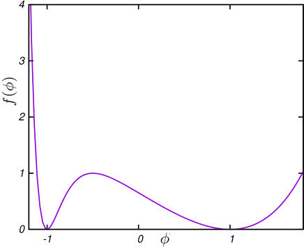
Figure 1: Shape of the mesoscopic free energy density (14)
with , , and .
Numerical simulations.—
Because the cut-off dependence of the formula (13)
is rather striking, we now confirm this result using numerical simulations.
We note that when .
Therefore, an asymmetric landscape of is necessary for
the appearance of the entropic driving force. On the basis of this fact,
we assume the local free energy density is given by
(14)
as in Ref. [8].
Here, satisfies the condition
that and . In Fig. 1, we show the form of the local free energy density . It can be seen that
the potential is highly asymmetric, i.e., .
Examples of asymmetric free energy density were presented in Refs. [21, 22].
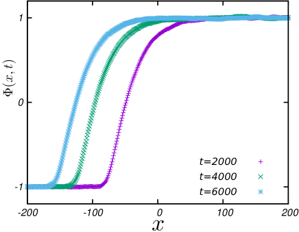
Figure 2:
Time evolution of the pattern averaged in the -direction.
The free energy density is the same as that in Fig. 1.
The other parameter values are , , ,
and . Noting that and for these
parameters, we choose and [24].
We define a discrete model on a square lattice with a spatial mesh size of , considering that should be smaller than and .
The discrete model is obtained by discretizing (2), where is replaced by the finite difference Laplacian.
For the initial condition
(15)
the stochastic time evolution is performed using the Heun method.
We then measure
(16)
which describes the -profile averaged in the -direction.
In Fig. 2, we show an example of
for several values of .
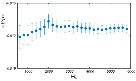
For the interface position defined by ,
we define a time-averaged velocity as
(17)
where is chosen to be much larger than the relaxation time
to the steady propagating state. In Fig. 3, we plot
the expectation value of , which gives the numerically estimated
value of .
We then confirm that is proportional to for [24].
Figure 3: as a function of .
The parameter values are the same as those in Fig. 2.
. Eighty samples are used to estimate with
error-bars.
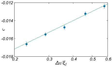
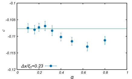
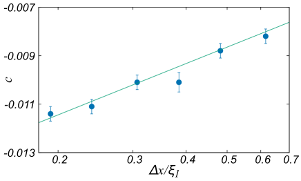
We now perform the same calculation for systems with different
values of . The results are displayed in Fig. 4.
It is observed that
does not go to a definite value as becomes
smaller under the condition that ,
which is in contrast with the one-dimensional case.
To compare the numerical data with the theoretical result,
we overlay the graph of (9) with (13)
in Fig. 4, where we choose
(18)
which corresponds to the largest magnitude of the wave vector
in the numerical simulations.
We find that the theoretical calculation is consistent
with the numerical simulations. We thus conjecture that
diverges in the limit even in
numerical simulations.
Figure 4: -dependence of the propagating velocity for
the system in two dimensions.
The parameter values are the same as those in Fig. 2.
The blue circles represent numerical results given by .
The green curve represents (9) with (13).
We checked the validity of the values of the numerical parameters
and [24].
Sketch of the derivation.—
We first take the limit .
Let be sufficiently small such that
the noise effect can be studied as a perturbation of
the deterministic system. To express this smallness,
we replace with , where is
a small dimensionless parameter.
When a perturbation is imposed on the stationary solution
, the response is divided into the interface
motion and the rest. That is, we express
the perturbation solution as
(19)
with the co-moving coordinate .
Assuming that is small and proportional
to , we introduce a large scaled coordinate as
, and define .
The time evolution of is described by
(20)
where represents the dependence of
and .
By substituting (19) and (20) into (2),
we can determine the statistical properties of , , and
. This calculation method is regarded as a generalization
of the method in Ref. [14] to stochastic systems.
The stationary propagation velocity is obtained as
.
We calculate and
(21)
This formula was derived in Ref. [23].
Now, from the time-reversal symmetry of the steady state in the co-moving frame,
we find that the integral of the numerator in (21) is
expressed as
using a function given by
where and . Finally, by evaluating ,
we obtain (11). The calculation result is immediately generalized
to -dimensional systems [24]. In particular, for the case , we obtain
(10).
Concluding remarks.—
We have derived the formula (9) with (11)
for the entropic driving force in the mesoscopic model (2).
Although we have studied the case , it is straightforward to
derive the propagation velocity for as , which is denoted by .
We have found that the entropic force singularly depends on the microscopic
cut-off of the mesoscopic model (2) in two dimensions.
This discovery suggests the need for further study.
The most important challenge is an experimental observation
of the entropic force in two or three dimensions.
As an experimental system, we propose to study a spin-crossover complex
where high-spin and low-spin states can coexist with an
interface [9].
Since curvatures of the free energy at these states
are different, we expect the entropic contribution of the force
generating the interface propagation. Here, through the measurement
of the space-time correlation of order parameter fluctuations,
and the correlation lengths are evaluated.
By measuring directly at sufficiently low temperatures and , we may estimate the value of by using
with the assumption that in the low temperature region does not depend on .
From the theoretical viewpoint, it is significant to generalize
our formula (9) for studying various systems such as
conserving systems [28] and
out-of-equilibrium systems [29, 30, 31]. More
fundamentally, in pursuit of a microscopic understanding of the cut-off,
one can attempt to consider the derivation of the mesoscopic
description from more microscopic systems such as lattice models
[32] or Hamiltonian systems [33]. Although there have
been many related studies since Ref. [34], the explicit
determination of coefficients of the mesoscopic model is not easy as argued in Ref. [35]. To develop a theory explaining
the cut-off dependence based on a microscopic description should be
another goal of non-equilibrium statistical mechanics.
As another direction of study, the universality class of
stochastic interface motion will be explored by studying the fluctuation
properties of the interface motion. With regard
to this problem, we point out that the microscopic cut-off dependence
observed in the Kardar-Parisi-Zhang equation [26, 27] comes from a non-linear term
that is not relevant in our problem [24]. Thus, the microscopic
cut-off dependence reported in this Letter has never been studied so far.
The authors thank K. Kanazawa and K. Saito for useful comments.
This study was supported by JSPS KAKENHI (Grant Numbers JP19H05795,
JP20K20425, and JP22H01144).
References
[1]
L. D. Landau and E. M. Lifshitz, Fluid Mechanics, Course of Theoretical Physics, Vol. 6 (Addision-Wesley, Reading, MA, 1959).
[2]
D. Forster, D. R. Nelson, and M. J. Stephen, Large-distance and long-time properties of a randomly stirred fluid, Phys. Rev. A 16, 732 (1977).
[3]
L. P. Kadanoff and J. Swift, Transport Coefficients near the Liquid-Gas Critical Point, Phys. Bev, 166, 89 (1968).
[4]
K. Kawasaki, Kinetic equations and time correlation functions of critical fluctuations, Ann. Phys. (N. Y.) 61, 1-56 (1970).
[5]
P. C. Hohenberg and B. I. Halperin, Theory of dynamic critical phenomena, Rev. Mod. Phys. 49, 435 (1977).
[6]
P. Bak, S. Krinsky, and D. Mukamel, Phys. Rev. Lett.
36, 52 (1976).
[7]
K. G. Wilson and J. Kogut, The renormalization group and the expansion, Phys. Rep. 12, 75-199 (1974).
[8]
G. Costantini and F. Marchesoni, Asymmetric Kinks: Stabilization by Entropic Forces, Phys. Rev. Lett. 87, 114102 (2001).
[9]
K. Boukheddaden, M. Sy, M. Paez-Espejo, A. Slimani, and F. Varret, Dynamical control of the spin transition inside the thermal hysteresis
loop of a spin-crossover single crystal, Physica B 486, 187-191 (2016).
[10]
Y. Pomeasu, Front motion, metastability and subcritical bifurcations in hydrodynamics, Physica D 23, 3-11 (1986).
[11]
C. Cattuto, G. Costantini, T. Guidi, and F. Marchesoni, Elastic strings in solids: Discrete kink diffusion, Phys. Rev. B 63, 094308 (2001).
[12]
J. F. Currie, J. A. Krumhansl, A. R. Bishop, and S. E. Trullinger, Statistical mechanics of one-dimensional solitary-wave-bearing scalar fields: Exact results and ideal-gas phenomenology, Phys. Rev. B 22, 477 (1980).
[13]
R. M. DeLeonardis and S. E. Trullinger, Exact kink-gas phenomenology at low temperatures, Phys. Rev. B 22, 4558 (1980).
[14]
Y. Kuramoto, Instability and Turbulence of Wavefronts in Reaction-Diffusion Systems, Prog. Theor. Phys. 63, 1885-1903 (1980).
[15]
Y. Kuramoto, On the Reduction of Evolution Equations in Extended Systems, Prog. Theor. Phys. Suppl. 99, 244-262 (1989).
[16]
E. Meron, Pattern formation in excitable media, Phys. Rep. 218, 1-66 (1992).
[17]
M. C. Cross and P. C. Hohenberg, Pattern formation outside of equilibrium, Rev. Mod. Phys. 65, 851 (1993).
[18]
S.-i. Ei and T. Ohta, Equation of motion for interacting pulses,
Phys. Rev. E 50, 4672-4678 (1994).
[19]
A. Karma and W.-J. Rappel, Quantitative phase-field modeling of dendritic growth in two and three dimensions, Phys. Rev 57, 4323 (1997).
[20]
M. Hiraizumi and S.-i. Sasa, Perturbative solution of a propagating interface in the phase field model, J. Stat. Mech. 103203 (2021).
[21]
K. Boukheddaden, M. Nishino, S. Miyashita, and F. Varret, Unified theoretical description of the thermodynamical properties of spin crossover with magnetic interactions, Phys. Rev. B 72, 014467 (2005).
[22]
S. Miyashita, Y. Konishi, H. Tokoro, M. Nishino, K. Boukheddaden and F. Varret, Structure of Metastable States in Phase Transitions with High-Spin
Low-Spin Degree of Freedom, Prog. Theor. Phys. 114,
719-734 (2005).
[23]
M. Iwata and S.-i. Sasa, Theoretical analysis for critical fluctuations of relaxation trajectory near a saddle-node bifurcation, Phys. Rev. E 82, 11127 (2010).
[24]
See Supplemental Material at [URL will be inserted by publisher] for
detailed arguments of numerical simulations, derivations, and some
remarks, which includes Refs. [25, 26, 27].
[25]
K. Kawasaki and T. Ohta, Kinetic Drumhead Model of Interface. I, Prog. Theor. Phys 67, 147-163 (1982).
[26]
M. Kardar, G. Parisi, and Y.-C. Zhang, Dynamic Scaling of Growing Interfaces
Phys. Rev. Lett. 56, 889 (1986).
[27]
K. A. Takeuchi, An appetizer to modern developments
on the Kardar–Parisi–Zhang universality class, Physica
A 504, 77 (2018).
[28]
J. W. Cahn and J. E. Hilliard, Free Energy of a Nonuniform System. III. Nucleation in a Two‐Component Incompressible Fluid, J. Chem. Phys. 31, 688 (1959).
[29]
P. Panja, Effects of fluctuations on propagating fronts, Phys. Rep. 393, 87-174 (2004).
[30]
A. Rocco, L. Ramírez-Piscina, and J. Casademunt, Kinematic reduction of reaction-diffusion fronts with multiplicative noise: Derivation of stochastic sharp-interface equations, Phys. Rev. E 65, 056116 (2002).
[31]
A. Lemarchand and B. Nowakowski, Do the internal fluctuations blur or enhance axial segmentation?, EPL 94, 48004 (2011).
[32]
H. Spohn, Long range correlations for stochastic lattice gases in a non-equilibrium steady state, J. Phys. A: Math. Gen. 16, 4275 (1983).
[33]
M. Kobayashi, N. Nakagawa, and S.-i. Sasa, Control of metastable states by heat flux in the Hamiltonian Potts model, Phys. Rev. Lett. 130, 247102 (2023).
[34]
R. Zwanzig,
Memory Effects in Irreversible Thermodynamics,
Phys. Rev. 124, 983–992, (1961).
[35]
K. Saito, M. Hongo, A. Dhar, and S.-i. Sasa, Microscopic Theory of Fluctuating Hydrodynamics in Nonlinear Lattices, Phys. Rev. Lett. 127, 010601 (2021).
Supplemental Material:
Microscopic cut-off dependence of an entropic force in interface propagation of stochastic order parameter dynamics
Yutaro Kado and Shin-ichi Sasa
In the first part of Supplemental Material (SM),
we derive (11) following the sketch of
derivation in the main text. In the second part of
SM, we present details of numerical simulations.
I I. Derivation of the main result
In Sec. I A, we briefly explain
a setup of perturbation theory. In Sec. I B,
we introduce some quantities that are useful in the analysis.
In Sec. I C, we review the derivation of (21).
The arguments to this point are well-known. Section I D
is the technical highlight, which has not been reported in
literature, as far as we know. Using the time-reversal symmetry,
we derive (22). In Sec. I E, we obtain (11) by calculating
fluctuations. In Sec. I F, we address some remarks on
the theoretical calculation.
Throughout the first part of SM,
we set without loss of generality.
I.1 A. Setup
We rewrite (2) in the main text as
(S1)
Since we take the limit , the boundary
conditions in the -direction become
as and
as .
We study the case in (4) in the main text. That is,
we assume that there exists satisfying
(S2)
To express the smallness of noise intensity,
we replace by , where is a
small dimensionless parameter. Thus, satisfies
(S3)
As presented in (19) in the main text,
we express a perturbation solution for as
(S4)
with the co-moving coordinate ,
where represents an interface position for each at time .
Assuming that is small and proportional to ,
we introduce a large scaled coordinate and define
. The time evolution of is
described by
(S5)
where represent the dependence of and
. We substitute (S4)
and (S5) into (S1). In this calculation,
we note
(S6)
with .
We then collect
terms proportional to . From this, we can determine
and . Next, collecting terms proportional to
, we derive . The propagation velocity
is given by
(S7)
Below, we explain these calculations.
I.2 B. Preliminaries
For later convenience,
we introduce some useful quantities, a linear operator ,
projection operators and , noises ,
, and .
I.2.1 1. Operators
We first define the linear operator
(S8)
which describes the linear dynamics of perturbations
around . Setting ,
we can confirm
(S9)
from the space-translation symmetry of the system.
Formally, corresponds to the Goldstone mode associated
with the translation symmetry breaking by the solution .
Physically,
describes the interface mode.
We next define the projection to the mode by
(S10)
for , where represents the inner product given by
(S11)
for functions and defined on
.
We also define .
I.2.2 2. Noises
For a given noise , we define
(S12)
Statistical properties of are characterized
by =0 and
(S13)
For this noise , we consider the projected noise
. The noise intensity
of is calculated as
(S14)
From this result, we immediately obtain
(S15)
I.3 C. Derivation of (21)
In this section, we derive (21) in the main text.
As described in Sec. I C, we substitute
(S4) and (S5)
into (S1). Then, collecting terms
proportional to , we obtain
(S16)
with
(S17)
Because ,
there exists a solution to the linear equation (S16)
only when . To have a consistent perturbation solution,
we impose this condition, which is referred to as the solvability
condition. The solvability condition leads to
We set and . In this section,
we evaluate
which is connected to by (S33) and (S32).
We fix a sufficiently large . It is reasonable to
assume that fluctuations at a point
are equivalent to those at a point of the homogeneous system
with without any interfaces, because the
point is far from the interface.
With this assumption, it is easy to analyze (S19).
We have the following estimations:
(S38)
(S39)
(S40)
where .
It should be noted that the results are independent of .
Here, by substituting into these
equations and combining them as the form (S31),
we obtain
(S41)
By substituting them into (S33) and (S32),
we obtain (11) and (12) in the main text.
I.6 F. Remarks
I.6.1 1. Mobility
To numerically calculate the right-hand side of (9) in the main text,
we have to estimate the value of the right-hand side of (6).
Using (S2), we first obtain
(S42)
where we have used
, , and .
This result leads to
(S43)
The right-hand side of (S43) is numerically estimated as
for the local free energy density displayed
in Fig. 1 of the main text.
I.6.2 2. Generalization
It is straightforward to generalize
the above arguments to the -dimensional system. We can calculate
(S44)
where .
In particular, for the one-dimensional system, we have
(S45)
(S46)
These are (10) and (12) in the main text.
For the three-dimensional system, we have
(S47)
I.6.3 3. Previous Studies
The calculation method presented in this paper
is regarded as a stochastic generalization of the method
used in the analysis of deterministic equations [1].
The formulation was reported in Ref. [2].
For the one-dimensional system, the result of is the same as
that obtained in the previous study [3], although
their calculation method is different from ours.
The advantage of our method is that we can easily analyze the
-dimensional system.
We also note that our result (S30) with (S31)
can be obtained by using an expression for reported in
Ref. [4]. However, this expression is not correctly
derived. Specifically, we should prove the non-trivial relation
(S29) to derive the expression, but there
are no arguments for the proof in Ref. [4].
I.6.4 4. Universality Class
A one-dimensional growing interface in a two-dimension space
is often described by the Kardar-Parisi-Zhang (KPZ) equation [5, 6]
(S48)
with the Gaussian white noise satisfying
(S49)
The average drift velocity is then given by
(S50)
From the fluctuation property of the KPZ equation, it can be
easily seen that shows a ultra-violet
divergence.
However, in the present problem, in the lower order of
the perturbation theory, as discussed in Sec. I C.
Indeed, according to our perturbation theory, we have ,
, , and . We thus confirm
that .
Thus, as far as we focus on the region , the non-linear term
is not relevant.
Our discovery is that exhibits the ultra-violet divergence
which is qualitatively different from the divergence observed in the KPZ
equation. It is an important problem to
clarify the universality class of our model.
II II. Details of Numerical Simulations
In Fig. 4 of the main text, we report the numerical result of the propagating velocity in the two-dimensional system. In this section, we explain
the details of the numerical simulations. In Sec. II A,
we first introduce the numerical scheme we employed.
In Sec. II B, we show the numerical result for
the one-dimensional system to demonstrate that the parameter
values chosen in the main text are appropriate. In Sec. II C,
we show supporting data for the results presented in the main text.
II.1 A. Numerical scheme
We discretize as , where and are
integers satisfying and .
We note that and ,
where is a space interval. Let be defined
by . We define the discrete Laplacian as
(S51)
where we impose the periodic boundary conditions in the -direction
and the Dirichlet boundary conditions in the -direction.
We then discretize time as , where is a non-negative
integer and is a time interval.
Let represent .
The time evolution of
is given by the Heun method defined by
(S52)
where and are given by
(S53)
and
(S54)
with
(S55)
Here, obeys the Gaussian distribution with zero mean and
unit variance.
II.2 B. Numerical result for
The numerical parameters used in the main text are ,
, and for the system with ,
, , , and . Note that
the correlation lengths of fluctuations in the bulk regions are
and . In this subsection, we show the numerical results in the
one-dimensional system to demonstrate that these numerical parameters
are appropriate. The parameter values of the system are the same as the
two-dimensional case except for . The numerical simulation method
for the one-dimensional system is basically the same as the two-dimensional
case.
First, we study a time-interval dependence of the propagation velocity.
We define a dimensionless time interval
(S56)
The diffusion term causes the instability when .
In Fig. S1, we show the propagating velocity
for various values of with fixed.
We then find that the data for small converges to the
formula of (8) in the main text. Since
for the numerical results presented in the main text,
we judge that our choice of the numerical parameters is
appropriate.
Figure S1:
-dependence of the propagating velocity for the system
in one dimension. The blue circles represent numerical results.
The green line represents (8) in the main text.
Five hundred samples are used to estimate with error-bars.
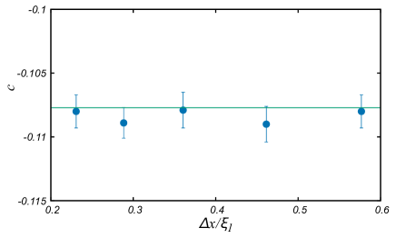
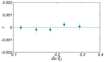
Next, we study a space-interval dependence of the propagation velocity.
In Fig. S2, we show the propagating velocity
for various values of with
fixed. Note that takes smaller values than in the range
of we study. We find that the numerical result
is consistent with the theory. This gives another evidence that our
numerical simulations are reliable.
Figure S2:
-dependence of the propagating velocity for
the system in one dimensions. The blue circles represent numerical results.
The green line represents (8) in the main text.
Five hundred samples are used to estimate with error-bars.
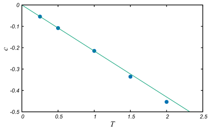
Finally, in Fig. S3, we show the temperature dependence
of . We observe that is proportional to when is less
than 1.0.
Figure S3:
Temperature dependence of the propagating velocity .
The blue circles represent the numerical results
for the system with and .
Five hundred samples are used to estimate with error-bars.
The green line represents the theoretical result (8) in the main text.
II.3 C. Supplemental data for
In this subsection, we investigate the parameter dependence
of the propagation velocity for the system with .
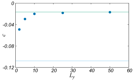
We first study the -dependence of to
check whether chosen for Fig. 4 is sufficiently large.
In Fig. S4, we plot for various values of .
We find that increases as increases and that
converges to the value of the formula (9) of the
two-dimensional system in the main text. We thus judge that
is sufficiently large.
Figure S4:
-dependence of the propagating velocity for the
system in two dimensions. The blue circles represent numerical results.
The green line represents the formula (9) for the two-dimensional
system in the main text, while the light blue line represents the formula
for the one-dimensional system (8) in the main text.
Fifty samples are used to estimate with error-bars.
The numerical parameter values are chosen as ,
and .
Next, we study the propagation velocity for another value of
and to check the generality of the cut-off dependence.
The numerical parameters are the same as those in Fig. 4 in the main
text except for (i) or (ii) , and .
Note that the correlation lengths of fluctuations in the bulk regions
are and for the case (i) and
for the case (ii).
In Figs. S5 and S6,
we show the propagating velocity for various values of
with fixed.
Note that takes smaller values than for the case (i)
and for the case (ii). We find that the numerical results
are consistent with our theoretical calculation.
Figure S5:
Similar graph as Fig. 4 in the main text, where
while the other parameter values are the same as
those for Fig. 4. Eighty samples are used to estimate
with error-bars. Figure S6:
Similar graph as Fig. 4 in the main text, where the symmetric
potential is used while the other parameter values are the same as
those for Fig. 4. One hundred samples are used to estimate
with error-bars.
References
[1]
Y. Kuramoto, Instability and Turbulence of Wavefronts in Reaction-Diffusion Systems, Prog. Theor. Phys. 63, 1885-1903 (1980).
[2]
M. Iwata and S.-i. Sasa, Theoretical analysis for critical fluctuations of relaxation trajectory near a saddle-node bifurcation, Phys. Rev. E 82, 11127 (2010).
[3]
G. Costantini and F. Marchesoni, Asymmetric Kinks: Stabilization by Entropic Forces, Phys. Rev. Lett. 87, 114102 (2001).
[4]
K. Kawasaki and T. Ohta, Kinetic Drumhead Model of Interface. I, Prog. Theor. Phys 67, 147-163 (1982).
[5]
M. Kardar, G. Parisi, and Y.-C. Zhang, Dynamic Scaling of Growing Interfaces
Phys. Rev. Lett. 56, 889 (1986).
[6]
K. A. Takeuchi, An appetizer to modern developments on the Kardar-Parisi-Zhang universality class, Physica A 504, 77 (2018).