HyperTab: Hypernetwork Approach for Deep Learning on Small Tabular Datasets

Abstract

Deep learning has achieved impressive performance in many domains, such as computer vision and natural language processing, but its advantage over classical shallow methods on tabular datasets remains questionable. It is especially challenging to surpass the performance of tree-like ensembles, such as XGBoost or Random Forests, on small-sized datasets (less than 1k samples). To tackle this challenge, we introduce HyperTab, a hypernetwork-based approach to solving small sample problems on tabular datasets. By combining the advantages of Random Forests and neural networks, HyperTab generates an ensemble of neural networks, where each target model is specialized to process a specific lower-dimensional view of the data. Since each view plays the role of data augmentation, we virtually increase the number of training samples while keeping the number of trainable parameters unchanged, which prevents model overfitting. We evaluated HyperTab on more than 40 tabular datasets of a varying number of samples and domains of origin and compared its performance with shallow and deep learning models representing the current state-of-the-art. We show that HyperTab consistently outranks other methods on small data (with statistically significant differences) and scores comparable to them on larger datasets.

I Introduction

Deep learning has already gained great success in various fields, such as computer vision [1], natural language processing [2], and video analysis [3] or reinforcement learning [4]. However, in tabular data analysis, deep learning methods are not as popular as in other areas. Somehow, although neural networks were first created with this aim in mind, it turned out that their performance on tabular data is subpar to other, much simpler algorithms [5], [6].

There are many potential reasons for this. Modern deep learning architectures designed for computer vision, such as convolutional networks [7] or vision transformers [8], emerged after years of research to create inductive biases that match invariances and spatial dependencies of image data. Finding corresponding invariances in tabular data is hard, which makes the fully-connected architectures the first choice for tabular datasets. Moreover, typical computer vision models containing millions of parameters are trained on an enormous amount of data coming from common domain, such as photographs, which allows them to discover sophisticated patterns without overfitting. In real-world settings, small tabular datasets are ubiquitous. If the dimension of data is relatively large compared to the number of examples, then the fully-connected networks rapidly overfit, which prevents from using deeper architectures.

In our work, we take inspiration from classical ensemble models, such as Random Forests [9] or random subspace method [10], which significantly improve the generalization ability of decision trees even for small high-dimensional data. Instead of training an individual model, Random Forests generate an ensemble of trees, each one taking into account a selected subset of features and specialized for a subset of samples. The feature subsetting plays the role of data augmentation, which generates multiple views of a single instance, allowing the number of available data to be increased. Following the above reasoning, we introduce HyperTab, a novel and effective technique for building an ensemble of neural networks for learning from small tabular datasets, see Figure 1. HyperTab combines the ensembling strategy with the augmentation mechanism, which significantly increases the number of training data and, consequently, allows the use of larger network architectures. To meet the requirement that the augmentation is a class-invariant transformation (the class label does not change after applying the augmentation), we use the feature subsetting as the admissible augmentations.

HyperTab follows the hypernetwork approach, in which a single hypernetwork builds an ensemble of target networks. Given the augmentation identifier (subset of features), the hypernetwork generates the parameters of the target network, which is crafted to process data points transformed by this augmentation. In the case of feature subsetting augmentations, each target network operates on a lower-dimensional view, where data are represented by the subset of features. In this way, we have as many training examples as the number of $[augmentation,example]$ pairs. Moreover, since the parameters of target networks are not optimized but returned by the hypernetwork, we significantly reduce the number of trainable parameters compared to the size of the ensemble. The only trainable parameters are the weights of the hypernetwork. In consequence, we obtain an effective and modern framework for constructing a deep learning model for challenging cases of small tabular datasets. Finally, generating individual target networks for specific subsets of features using a single hypernetwork is also a way to automatically design network architectures, which include internal dependencies between coordinates.

To validate our approach, we used a diverse benchmark of 22 public tabular datasets and 20 real microbial data. Our experiments clearly confirm that HyperTab gives a superior performance on small datasets – its advantage over current state-of-the-art models being statistically significant. In the case of large datasets, where the problem of overfitting is reduced, HyperTab works similarly to other algorithms. In addition to benchmark tasks, we performed a detailed analysis of HyperTab, which allows us to understand how the selection of hyperparameters affects its performance.

Our contributions can be summarized as follows:

• We introduce HyperTab, which effectively builds an ensemble of neural networks using the hypernetwork approach.

• We apply an augmentation strategy based on feature subsetting, which is consistent with the characteristic of tabular data, and allows for virtually increasing the number of training samples.

• We evaluate HyperTab on various datasets and show that it obtains the state-of-the-art on small data sets.

We make a Python package with the code available to download at https://pypi.org/project/hypertab/.

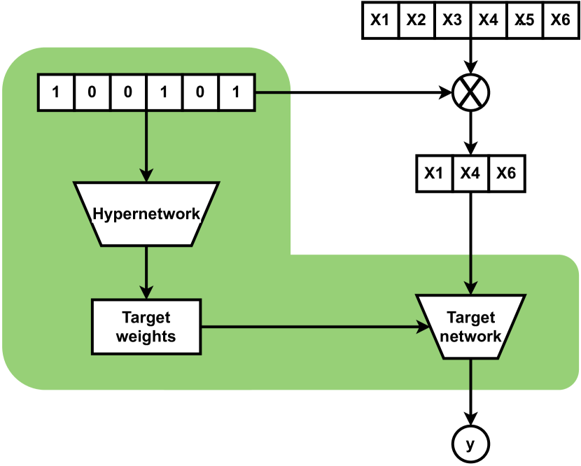
Figure 1: A general HyperTab architecture. Given a binary mask representing a subset of features (augmentation), the hypernetwork generates the weights to the target network, which operates on a lower-dimensional view of data determined by the mask. The response of HyperTab is based on multiple target networks generated for individual augmentations.

II Related work

II-A Hypernetworks

Hypernetwork is hardly a new concept – having been introduced in [11] they have already been successfully used in various domains. In general, hypernetworks are an effective alternative to conditional neural networks [12] – the condition represents the input to the hypernetwork, which generates the weights of the target networks responsible for solving a target task. Hypernetworks appear frequently in the meta-learning literature [13]. In [14], hypernetworks were used to tackle the problem of catastrophic forgetting – an observation that networks that are trained sequentially on multiple tasks tend to vastly underperform in comparison to task-specific training. The authors of [15] and [16] use hypernetworks to construct a functional representation of images, in which we can inspect the image at various resolutions and perform on it arbitrarily continuous operations. [17] shows that hypernetworks can also be used to create generative models for 3D point clouds.

II-B Augmentations

Data augmentation is a key component of current deep learning models, which allows learning meaningful representation even in a self- or semi-supervised setting. Although there is a standard set of augmentations for computer vision or natural language [18], there is no consensus on how to select proper augmentations for tabular datasets, in which spatial or semantic structures usually do not exist. One of the standard approaches relies on corrupting data, e.g. by adding Gaussian noise [19]. Alternatively, we can replace the values of selected features (determined by the mask vector) with the dummy values [20]. We can either zero out them, perform the imputation using the mean or median, as well as use values taken from other instances. Although analogous strategies have been applied in self-supervised learning or in the definition of pretext tasks [21], [22] [20], they do not guarantee that the class label remains unchanged after such augmentations. The authors of [23] applied mix-up training by mapping samples to a low-dimensional latent space and encouraging interpolated samples to have high similarity within the same labeled class. In our paper, we decided to construct a lower-dimensional view of the original data by randomly selecting a subset of features, which is analogous to the idea of the random subspace method. However, instead of training many individual models, we employ the hypernetwork, which is responsible for generating weights to target models. In this way, we reduce the number of trainable parameters.

II-C Shallow models for tabular datasets

In contrast to computer vision or natural language processing, shallow models, such as Support Vector Machines [24], [25], Random Forests [26], [9], and Gradient Boosting [27], are usually the first choice for learning from tabular datasets. In particular, the family of Gradient Boosting algorithms [27], including XGBoost [28], LightGBM [29], CatBoost [30], and GOSDT [31] achieve impressive performance and frequently exceed the performance of deep learning models. Both Gradient Boosting as well as Random Forests generate an ensemble of weak learners composed of decision trees, but they differ in the way those trees are built and combined.

II-D Deep learning on tabular data

To take advantage of the flexibility of neural networks, various architectures have recently been proposed to improve their performance on tabular data. Inspired by CatBoost, NODE performs a gradient boosting of oblivious decision trees, which is trained end-to-end using gradient-based optimization [32]. The aim of Net-DNF is to introduce an inductive bias in neural networks corresponding to logical Boolean formulas in disjunctive normal forms [33]. It encourages localized decisions, which involve small subsets of features. TabNet uses a sequential attention mechanism to select a subset of features, which are used at each decision step [34]. Hopular is a deep learning architecture in which every layer is composed of continuous modern Hopfield networks [35]. The Hopfield modules allow one to detect various types of dependencies (feature, sample, and target) and have been claimed to outperform concurrent methods of small and medium-sized datasets. The authors of [36] show that the key to boosting the performance of deep learning models is the application of various regularization techniques. They show that fully connected networks can outperform concurrent techniques by applying an extensive search on possible regularizers. Although authors of recent deep learning models often claim to outperform shallow ensemble models, other experimental studies seem to deny these conclusions, showing that XGBoost with careful hyperparameter tuning presents superior performance [5], [6].

In our paper, we are especially interested in overcoming the limitations of deep learning models on small tabular datasets. Although learning from tabular data also poses other challenges, such as encoding categorical features, we intentionally focus on that specific case. By taking advantage of feature subsetting used in decision tree ensembles and hypernetworks, we build a modern deep learning model which is especially suited for small sample problems.

III The HyperTab model

It has been widely noted [6] that tree-like ensemble methods often outperform deep learning algorithms on tabular datasets. Following this observation, we introduce HyperTab, which follows these algorithms and combines an implicit data augmentation with neural network ensembles to ensure its performance on small datasets.

III-A Model overview

HyperTab consists of two main components: hypernetwork $H$ and an ensemble of target networks $T_{j}$, for $j=1,\ldots,k$, see Figure 1. The hypernetwork takes the type of augmentation as input and returns the parameters of the target network, which is designed to use such an augmented view of data. Since augmentations are defined as feature subsetting, every target network operates on a lower-dimensional view of the data determined by selected coordinates. In contrast to typical neural network ensembles, the weights of target networks are not optimized directly using gradient descent but are generated by the hypernetwork. The only trainable parameters are the hypernetwork weights.

Such an approach is especially profitable for small datasets, because augmentations allow us to significantly increase the number of training examples. Instead of using raw data, we combine each data point with all types of augmentations, giving us $n\cdot k$ training examples, where $n$ is the number of examples, and $k$ denotes the number of augmentations. The number of trainable weights of HyperTab remains roughly the same as in typical fully connected neural networks processing original data.

In the following parts, we describe our approach in detail.

III-B Augmentations

It is not obvious how to construct augmentations suitable for tabular datasets. Augmentation is a class-invariant transformation of the data, which means that the class label cannot change after applying this transformation. Although recent progress in computer vision delivered a great variety of augmentations, there is no gold standard for tabular data. For this reason, we decided to restrict our attention to feature subsetting as admissible augmentations. By representing a data point by the subset of its features, we do not introduce noise, but only limit the information contained in the original data. Using an analogy with computer vision, feature subsetting is similar to random cropping. In our case, however, we reduce the dimension of the original data and completely eliminate features that have not been selected. An in-depth analysis of the relationship between feature subsetting and performance of the algorithm has been performed in section IV-C.

Let $X=\{x_{1},x_{2},\dots,x_{n}\}\subset\mathbb{R}^{d}$ be a tabular dataset, which we want to use in training a deep learning model. By $c\subset\{1,\ldots,d\}$, where $|c|=l$, we denote the subset of $l$ selected indices. Applying the augmentation defined by $c$ to a sample $x\in\mathbb{R}^{d}$ produces a vector $x[c]\in\mathbb{R}^{l}$, which represents a lower-dimensional view of the data point $x$.

III-C Construction of the ensemble

Every target network (component model in the HyperTab ensemble) is designed to process a specific augmented view of the data. More precisely, the target network $T_{c}:\mathbb{R}^{l}\to Z$ takes a lower-dimensional representation $x[c]$ and returns a vector $z\in Z$, e.g. logits in the case of classification. The vector $z$ can be converted to the final target value, e.g. a class label $y\in Y$. The augmentation $c$ determines the form of the target network $T_{c}$.

Instead of training an individual target network $T_{c}$ using gradient descent, we construct a central mechanism to generate the whole ensemble. That is, we use a hypernetwork $H$, which returns the parameters of the target network for a given type of augmentation. Since we work with feature subsetting, the augmentation $c\subset\{1,\ldots,d\}$ can be encoded as a binary mask $m\in\{0,1\}^{d}$ indicating the selected features, i.e.

$$m_{j}=\left\{\begin{array}[]{ll}1,&\text{ for }j\in c,\\ 0,&\text{ otherwise.}\end{array}\right.$$ (1)

The hypernetwork is thus a neural network ${H_{\psi}:\{0,1\}^{d}\to\Theta}$, which transforms a binary mask $m$ representing the augmentation $c$ to the weights $\theta_{c}$ of the target network $T_{\theta_{c}}$, i.e.

$$\theta_{c}=H_{\psi}(m).$$

The architecture is common for all target networks, but their weights are individually generated by the hypernetwork to process a specific augmented view of the data. Every target network returns:

$$z_{c}=T_{\theta_{c}}(x[c]),$$

given an augmented view of $x\in\mathbb{R}^{d}$.

III-D Training

To train HyperTab, we optimize the weights $\psi$ of the hypernetwork $H_{\psi}$. As mentioned, we do not optimize the parameters of the target networks directly, but only the weights of hypernetwork.

In a training step, we take a minibatch of augmentations $\mathcal{B}_{c}=\{c_{1},\ldots,c_{a}\}$, where $c_{j}\subset\{1,\ldots,d\}$ such that ${|c_{j}|=l<d}$, and define the corresponding masks ${m_{j}\in\{0,1\}^{d}}$ as in (1). Using the hypernetwork, we generate the weights of the target networks $\theta_{j}=H_{\psi}(m_{j})$. Every target network is then applied to the minibatch of data points $\mathcal{B}_{x}=\{x_{1},\ldots,x_{b}\}$ producing partial predictions $z_{ij}=T_{\theta_{j}}(x_{i}[c_{j}])$, for $i=1,\ldots,b$ and $j=1,\ldots,a$. Vectors $z_{ij}$ are compared to true targets $y_{i}$ via a given loss function $\mathcal{L}(y_{i},z_{ij})$, e.g., cross-entropy with softmax in the case of classification. The loss is minimized by changing the parameters $\psi$ of the hypernetwork $H_{\psi}$ using gradient descent.

As can be seen, a training sample is a pair of augmentation and data point. As a consequence, we have as many training samples as the number of data points times the number of augmentations. This is especially useful for small datasets because we can significantly increase the number of training data. Since the number of trainable network weights is comparable to that of a typical neural network, our approach prevents the model from overfitting.

III-E Inference

Once trained, the hypernetwork $H$ can produce the ensemble of weak learners $\theta_{j}=H_{\psi}(m_{j})$, where $m_{j}$ is a mask corresponding to the augmentation $c_{j}$, for $j=1,\ldots,a$. The final prediction for a given sample $x\in\mathbb{R}^{d}$ is calculated as the average of the predictions of the target networks taken over all augmentations:

$$z=\frac{1}{a}\sum_{j=1}^{a}T_{\theta_{j}}(x[c_{j}]).$$

We emphasize that $z_{c}=T(x[c])$ is the result of the last layer of the target network, for example, logits in the case of classification. We can also use different aggregation methods, but the mean pooling applied to logits makes HyperTab robust to the noisy augmentations containing irrelevant features, as shown in Section IV-C.

IV Experiments

IV-A Benchmark

Experimental setup

In order to thoroughly check the potential of HyperTab, we check its performance on multiple datasets coming from diverse domains. For transparency, we consider classification problems, but HyperTab can also be applied to regression tasks. We distinguish small datasets, in which the number of samples is less than 1k, and larger datasets with more than 1k samples. Since the construction of HyperTab is suitable for a small sample problem, we expect it to reach the state-of-the-art at least in the first group of datasets. An overview of the datasets can be found in Table 1 of the Supplementary Materials.

TABLE I: Performance of the algorithms on: (top) small datasets ($n\leq 1k$); (bottom) medium and large datasets ($n>1k$). We report the average of 5 runs and the standard deviation in brackets.

$\left.\begin{tabular}[]{p{3.5cm}p{1.7cm}p{1.7cm}p{1.7cm}p{1.7cm}p{1.7cm}}\hline\cr\hline\cr{Dataset}&{XGBoost}&{DN}&{RF}&{HyperTab}&{Node}\\ \hline\cr{Breast Cancer}&93.85 (1.44)&95.58 (1.04)&95.96 (1.52)&97.58 (1.11)&96.19 (1.11)\\ {Connectionist}&83.52 (3.94)&79.02 (5.29)&83.50 (5.55)&87.09 (5.53)&85.61 (3.48)\\ {Dermatology}&96.05 (0.89)&97.80 (1.17)&97.21 (1.66)&97.82 (1.24)&97.99 (1.20)\\ {Glass}&94.74 (3.91)&46.96 (2.56)&97.02 (1.51)&98.36 (3.21)&44.90 (1.90)\\ {Promoter}&81.88 (5.59)&78.91 (3.93)&85.94 (6.79)&89.06 (5.41)&83.75 (4.64)\\ {Ionosphere}&90.67 (2.75)&93.43 (3.72)&92.43 (2.60)&94.52 (1.47)&91.03 (1.79)\\ {Libras}&74.38 (4.55)&81.54 (3.99)&77.42 (3.88)&85.22 (2.92)&82.72 (3.27)\\ {Lymphography}&85.94 (3.14)&85.74 (5.28)&87.19 (4.33)&83.90 (5.01)&83.93 (5.82)\\ {Parkinsons}&86.35 (4.77)&74.96 (4.90)&86.84 (6.26)&95.27 (3.06)&80.20 (5.29)\\ {Zoo}&92.86 (8.75)&72.62 (4.96)&92.62 (7.97)&95.27 (3.06)&89.05 (3.98)\\ {Hill-Valley without noise}&65.53 (0.00)&56.39 (2.89)&57.33 (0.00)&70.59 (4.90)&52.71 (0.34)\\ {Hill-Valley with noise}&58.45 (0.00)&56.06 (1.65)&55.66 (0.00)&70.16 (3.25)&51.09 (0.26)\\ {OvarianTumour}&60.61 (8.80)&33.33 (0.00)&51.24 (7.53)&76.60 (4.48)&68.39 (10.82)\\ {Heart Disease (Cleveland)}&79.17 (7.24)&82.62 (4.50)&81.10 (3.89)&83.33 (2.54)&82.38 (4.59)\\ \hline\cr{Mean rank}&3.50&3.78&3.07&1.35&3.29\\ \hline\cr\end{tabular}\right\}\text{\rotatebox[origin={c}]{270.0}{small datasets}}$

$\left.\begin{tabular}[]{p{3.5cm}p{1.7cm}p{1.7cm}p{1.7cm}p{1.7cm}p{1.7cm}}{FashionMNIST}&89.45 (0.18)&89.01 (0.04)&88.04 (0.21)&90.22 (0.32)&89.51 (0.21)\\ {CNAE-9}&90.49 (2.05)&94.97 (0.77)&91.85 (1.36)&92.25 (2.55)&94.72 (1.17)\\ {Multiple Features}&98.03 (0.44)&98.27 (0.61)&98.98 (0.36)&98.12 (0.81)&98.58 (0.45)\\ {Devanagari}&72.03 (0.58)&75.24 (0.47)&71.15 (0.73)&78.92 (0.66)&78.20 (1.08)\\ {Volkert}&63.48 (0.37)&54.32 (1.51)&58.08 (0.26)&57.41 (2.38)&59.25 (0.99)\\ {Nomao}&96.50 (0.15)&95.71 (0.30)&95.83 (0.29)&95.53 (0.27)&95.23 (0.26)\\ {Fabert}&30.82 (0.78)&27.09 (0.26)&66.74 (1.00)&60.09 (0.09)&67.47 (1.19)\\ {Christine}&72.89 (0.98)&71.80 (0.53)&72.21 (0.98)&72.42 (2.19)&71.78 (1.24)\\ \hline\cr{Mean rank}&3.00&3.50&3.12&2.75&2.62\\ \hline\cr\hline\cr\end{tabular}\right\}\text{\rotatebox[origin={c}]{270.0}{larger datasets}}$

As an evaluation measure, we use balanced accuracy, which is especially designed for datasets with unbalanced classes. If the number of examples in each class is comparable, then balanced accuracy gives analogical scores to accuracy. In consequence, balanced accuracy is a perfect measure for our case, where datasets have diverse characteristics of classes.

The target networks in HyperTab are fully connected networks with a single hidden layer, with 5 to 50 neurons (defined by a hyperparameter). The hypernetwork is made up of 3 hidden layers with 128, 64, and 64 neurons. All activations are defined by the ReLU function. The number of augmentations and the number of selected features are hyperparameters chosen in a grid search procedure.

We test the performance of HyperTab along with two shallow algorithms and two deep learning models:

• RF (Random Forests). It is an ensemble of decision trees, which combines bagging with feature subsetting.

• XGBoost (Extreme Gradient Boosting). It is an implementation of the Gradient Boosting algorithm, which obtains the best performance among shallow machine learning models on tabular datasets.

• DN (Fully connected neural network with dropout regularization). We use a typical fully connected architecture with dropout regularization to avoid overfitting on small datasets. Dropout regularization before the first hidden layer makes the model similar to HyperTab, in which an individual model is trained on a subset of features.

• NODE (Neural Oblivious Decision Ensembles). It is a recent deep learning ensemble designed for tabular data, in which an individual decision tree is trained on a subset of features selected in a differentiable way. Comparing HyperTab with NODE allows one to verify different subsetting mechanisms in both methods and the way of generating the ensembles.

All algorithms are subject to the optimization of hyperparameters separately for each of the datasets. Grids specific to the algorithms can be found in the Appendix. To reduce random effects, we report mean and standard deviation across 5 runs of the algorithms. In particular, HyperTab is evaluated on 5 randomly selected sets of augmentations.

Results

The results presented in Table I (top) clearly show that HyperTab outperforms comparative methods on most examples of small datasets. In many cases, the difference between HyperTab and the second best-performing method is extremely high (e.g., in Parkinson, Hill-Valley, and Ovarian Tumor datasets), which confirms the advantages of HyperTab on small sample problems. There are two cases, where HyperTab does not obtain the best results: on Dermatology HyperTab is slightly worse than NODE, while on Lymphography the difference is greater.

To summarize the results, we apply statistical tests, see [37], specifically we used the Friedman test with Nemenyi post hoc analysis. For this purpose, we ranked all methods on every data set, i.e. the best-performing method got ranked 1, the second-best method got ranked 2, etc. Given a ranking of the methods, the analysis consists of two steps:

• The null hypothesis is made that all methods perform the same and the observed differences are merely random (the hypothesis is tested by the Friedman test, which follows a $\chi^{2}$ distribution,

• Having rejected the null hypothesis, the differences in ranks are analyzed by the Nemenyi test.

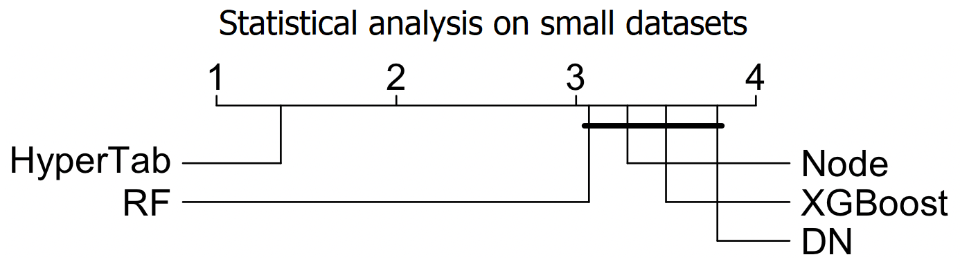
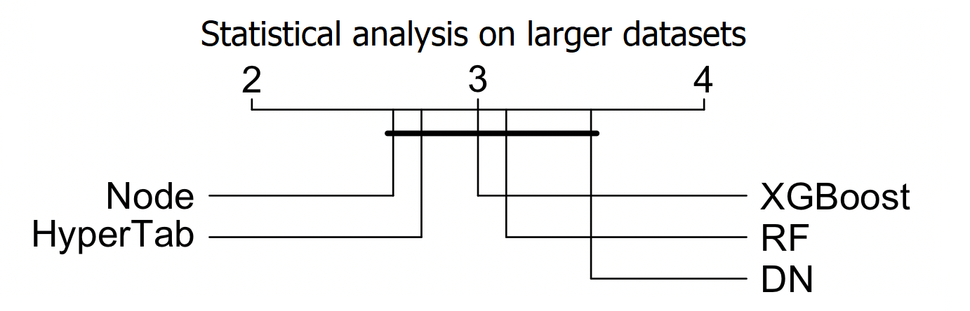
Figure 2: Statistical comparison of the methods on (top image) small datasets, (bottom image) lager datasets. A horizontal line connecting ranks shows which difference is not significant. HyperTab is confirmed to perform statistically better than comparative methods on small datasets.

Figure 2 (top) visualizes the results for a significance level of $p=0.05$. The x-axis shows the mean rank for each method. The groups of methods for which the difference in mean rank is not statistically significant are connected by horizontal bars. As can be observed, the difference between HyperTab and the second-best method is large. Moreover, the advantage of HyperTab over all algorithms is statistically significant.

For completeness, we also perform the evaluation on larger datasets. As can be seen in Table I (bottom), HyperTab performs on par with other methods, which confirms our initial hypothesis that HyperTab is best suited to small datasets. It obtains the highest results on two datasets. However, it is difficult to indicate the best algorithm across all datasets. The statistical test shows that the differences between algorithms are not significant, see Figure 2 (bottom).

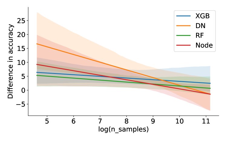
Figure 3: Difference in balanced accuracy between HyperTab and other methods in function of the number of samples. The advantage of HyperTab over all algorithms gradually increases as the number of samples decreases.

Figure 3 shows the relationship between the size of the dataset and the advantage of HyperTab over other methods. Specifically, we report the difference in performance between HyperTab and other methods in relation to the number of training samples. For transparency, we illustrate the estimated correlation. As can be seen, the advantage of HyperTab over all methods is greater for small samples and gradually decreases for larger datasets. We verified that the estimated correlation factor calculated for RF, the second-best performing method, with respect to the mean rank, is statistically significant with $p$-value equal to 0.05. It further supports our hypothesis that HyperTab is well suited for the classification of small tabular datasets. For large datasets, HyperTab is outperformed by NODE, which is one of the SOTA deep learning models for tabular data.

IV-B Use-case on microbial data

To further validate the performance of HyperTab, we tested it in a real-world scenario of metagenomic analysis. The purpose of this experiment is to assess what results we may expect to see once HyperTab is adopted by researchers from domains, who do not necessarily possess machine learning expertise.

Following the procedure described in [38], we start from an OTU table: operational taxonomical units of microorganisms present in the samples. We then apply a rudimentary feature selection method by discarding constant features and preprocess the data using ANCOMBC [39]. Since the procedure does not include tuning of the hyperparameters, we decided to also omit this step to replicate the real-world scenario as closely as possible.

We test HyperTab against three other algorithms commonly used in microbiome classification [38]: Random Forest, XGBoost, and Support Vector Classifier [40]. Our data consists of 20 datasets (summarized in the Supplementary Materials) that contain samples of the gut microbiome of patients with and without colorectal cancer. Their aim is to predict whether the patient has or does not have the aforementioned cancer based only on the composition of his gut microbiome.

Table II contains results for each of the datasets, and Figure 4 shows an overview of the scores. Once again, the results show that HyperTab consistently outperforms other methods on small datasets. The difference between HyperTab and the other methods is statistically significant.

TABLE II: Results on the metagenomic datasets. Each dataset’s name is derived from the first author’s surname and the year of publication.

Dataset	RF	SVC	XGBoost	HyperTab
FengQ_2015	0.84	0.87	0.81	0.98
GuptaA_2019	0.80	0.90	0.82	0.98
HanniganGD_2017	0.59	0.53	0.60	0.71
JieZ_2017	0.73	0.79	0.79	0.93
KeohaneDM_2020	0.60	0.44	0.49	0.50
LiJ_2017	0.49	0.50	0.47	0.58
NagySzakalD_2017	0.73	0.74	0.76	0.79
NielsenHB_2014	0.72	0.71	0.73	0.78
QinJ_2012	0.66	0.70	0.67	0.73
QinN_2014	0.89	0.90	0.87	0.91
RubelMA_2020	0.83	0.82	0.77	0.80
ThomasAM_2018a	0.62	0.54	0.71	0.66
ThomasAM_2018b	0.57	0.58	0.58	0.77
ThomasAM_2019c	0.70	0.67	0.78	0.88
VogtmannE_2016	0.72	0.56	0.70	0.64
WirbelJ_2018	0.72	0.85	0.76	0.92
YachidaS_2019	0.65	0.64	0.65	0.79
YuJ_2015	0.68	0.75	0.73	0.77
ZellerG_2014	0.68	0.75	0.68	0.66
ZhuF_2020	0.72	0.79	0.72	0.70
Mean rank	2.97	2.7	2.73	1.6

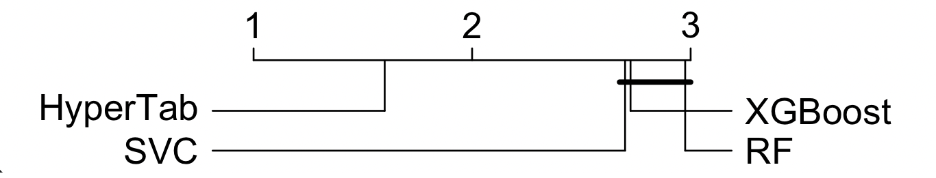
Figure 4: Analysis performed on microbial datasets shows that the difference between HyperTab and other algorithms is statistically significant.

IV-C Analysis

Dependence on the selection of augmentations

There are two main parameters that influence the performance of HyperTab: the number of augmentations (target models) and the number of features selected by each augmentation. In this experiment, we analyze their optimal values on two versions of the F-MNIST datasets.

First, we consider F-MNIST with only 100 samples (10 per class), which corresponds to the small sample problem. As can be seen in Figure 5 (top), the highest accuracy is obtained for a relatively large number of augmentations (80-200) and a small number of selected features (20-50). The large number of augmentations virtually increases the amount of training data, while the small number of selected features allows for constructing an ensemble with diverse target models.

To extend our analysis, we performed an analogical experiment on the full F-MNIST dataset containing 60k training samples. In contrast to the previous case, here we observe that the optimal performance is obtained for a smaller number of augmentations and a higher number of selected features, see Figure 5 (bottom). It may follow from the fact that for large datasets, we do not need to virtually increase the number of training samples as in the case of small sample problems. However, if the number of target networks is small, we need to use many features in each augmentation to provide enough information about the data.

In conclusion, the number of augmentations should be selected jointly with the number of features in each augmentation. For small-sample problems, it is beneficial to use a high number of augmentations with a small number of features, while for larger datasets this relation should be inverse.

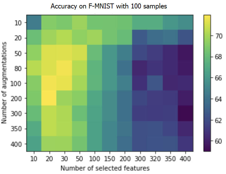
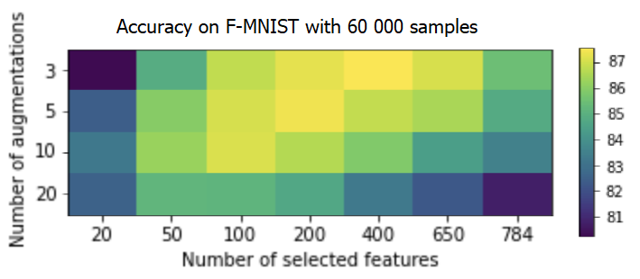
Figure 5: Influence of the number of augmentations and the number of selected features on the HyperTab performance analyzed on two versions of F-MNIST. Smaller datasets strongly benefit from the proposed ensembling strategy.

Dependence on irrelevant features

A natural question arises for HyperTab: What if there are few important features and many augmentations, by chance, happen to omit them? F-MNIST allows testing that phenomenon to some degree, since many of their pixels are purely background noise, and there is a high chance that for small number of selected features most of them will consist of noise only.

To further investigate this scenario, we devised a synthetic dataset with 50 columns, 49 of them randomly sampled from uniform distribution, and one being linearly dependent on the class of the example. The dataset has 5 unique classes and 50 samples. Each augmentation selects 10 features. We verified that only 17% of the augmentations use the informative feature, while the rest of them rely on noise for their predictions. Despite that, HyperTab was able to achieve perfect accuracy on this dataset.

To further analyze the reason behind this behavior, we inspect the predictions of individual target networks and present their histograms in Figure 6. We recall that the final prediction of HyperTab is calculated by taking the average of logits returned by the target networks. Our analysis shows that non-informative augmentations tend to craft target networks that are "uncertain" of their predictions. In order not to influence the voting too much, their logits are centered around 0. In contrast, target networks generated by augmentations containing the informative feature return confident predictions. Since the pooling layer operates on logits, HyperTab is able to reduce the effect of noisy models.

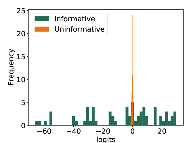
Figure 6: Histogram of target networks’ predictions (logits) calculated on informative and non-informative augmentations. Since HyperTab averages logits of target networks, the contribution of uncertain predictions generated by non-informative features is marginal compared to the confident scores obtained using informative features.

V Conclusion and future directions

This paper introduced HyperTab – a hypernetwork-based ensemble for deep learning on tabular datasets. Making use of feature subsetting as data augmentations, we virtually increase the number of training examples, keeping the number of trainable weights unchanged. This is especially profitable for small datasets, where typical deep learning models perform inferior to shallow methods. Our experiments clearly confirm that HyperTab obtains state-of-the-art results on small tabular datasets and performs on par with other methods on larger datasets.

We strongly believe that this paper may serve as a stepping stone for hypernetwork-based approaches for tabular data, as there are still many venues that can be further pursued. HyperTab relies on a random scheme for sampling augmentations. Although our analysis shows that HyperTab is robust to irrelevant features, we can introduce a differentiable procedure to learn an informative and diverse set of augmentations (potential ideas can be found in [32]). In addition to the classification task, we plan to consider regression problems. Our analysis shows that the target networks tend to produce near-zero output if they are uncertain of the correct result, suggesting that HyperTab may be suitable for regression.

Appendix A Datasets

Overview of basic tabular datasets is presented in Table III. Real-life metagenomic datasets are described in Table IV.

TABLE III: Overview of the datasets. Here, $n,d,k$ denote the number of samples, features, and classes, respectively. Domains abbreviations: CM - customer metadata, TF - text features, RD - radar data, CD - clinical data, PX - pixels, Co - compositional, S - synthetic, VF - video features, IF - image features, VoF - voice features, Bio - biological dataset, AF - animal features

Dataset	$n$	$d$	Dom.	Source	$k$
Christine	5418	1637	S	OpenML	2
CNAE-9	1080	857	TM	UCI	9
Connectionist	208	60	RD	UCI	2
Dermatology	366	33	CD	UCI	6
Devanagari	12912	784	PX	Kaggle	58
Fabert	8237	801	S	OpenML	7
FashionMNIST	70000	784	PX	-	10
Glass	214	10	Co	UCI	7
Heart Disease	303	14	CD	UCI	2
Hill-Valley	606	101	S	UCI	2
Ionosphere	351	34	RD	UCI	2
Libras	360	91	VF	UCI	15
Lymphography	148	18	IF	UCI	2
Mult. Features	2000	649	IF	UCI	10
Nomao	34465	120	CM	OpenML	2
OvarianTumour	283	54622	Bio	OpenML	3
Parkinsons	197	23	VF	UCI	2
Promoter	106	58	Bio	UCI	2
Volkert	58 310	181	S	OpenML	10
WBC	569	30	IF	UCI	2
Zoo	101	17	AF	UCI	7

TABLE IV: Overview of the metagenomical datasets.

Dataset	$n$	$d$
FengQ-2015	107	606
GuptaA-2019	60	308
HanniganGD-2017	55	292
JieZ-2017	385	683
KeohaneDM-2020	117	381
LiJ-2017	155	436
NagySzakalD-2017	100	438
NielsenHB-2014	317	606
QinJ-2012	344	651
QinN-2014	237	645
RubelMA-2020	175	370
ThomasAM-2018a	53	477
ThomasAM-2018b	60	503
ThomasAM-2019c	80	519
VogtmannE-2016	104	540
WirbelJ-2018	125	537
YachidaS-2019	509	718
YuJ-2015	128	575
ZellerG-2014	114	652
ZhuF-2020	171	480

Appendix B Hyperparameter optimisation

Each model’s specific set of hyperparameters was evaluated on the test set. Models were optimized across the following hyperparameters:

B-A XGBoost

XGBoost was optimized with two grids, each containing a different set of parameters. The optimal hyperparameters obtained from the first grid were later used when performing a search on the second grid.

First grid:

• $n\_estimators$: {50, 100, 250, 500, 1000, 3000},

• $max\_depth$: {2, 3, 5, 10, 15},

• $learning\_rate$: Log-Uniform distribution [1e-5,1e-1],

• $min\_child\_weight$: {1, 2, 4, 8, 16, 32}

• $gamma$: {0, 0.001, 0.1, 1}.

Second grid:

• $subsample$: {0.5, 0.6, 0.7, 0.8, 0.9, 1},

• $reg\_lambda$: Log-Uniform distribution [1e-5, 10] initial_value = 0,

• $reg\_alpha$: Log-Uniform distribution [1e-5, 10] initial_value = 0.

B-B NODE

• $layer\_dim$: {64, 128, 256, 512, 1024}. In some cases value 1024 was omitted due to memory issues (big datasets),

• $num\_layers$: Discrete uniform distribution [1, 5],

• $depth$: Discrete uniform distribution [2, 7],

B-C DN

• $epochs$: {100, 150},

• $dropout\_layer1$: {0.1, 0.3, 0.5, 0.7} (ordered),

• $dropout\_layer2$: {0.1, 0.3, 0.5, 0.7} (ordered),

• $dropout\_layer3$: {0.1, 0.3, 0.5, 0.7} (ordered),

• $dropout\_layer4$: {0.1, 0.3, 0.5, 0.7} (ordered),

• $learning\_rate$: {3e-5, 3e-4, 3e-3, 3e-2, 3e-1},

• $batch\_size$: {32, 64},

B-D RF

Common:

• $max\_features$: {’sqrt’, 0.2, 0.3, 0.5, 0.7},

• $criterion$: {’gini’, ’entropy’},

• $max\_depth$: {’default’, 2, 4, 8, 16},

Small datasets:

• $n\_estimators$: Discrete uniform distribution {50, 3000}, quantized to increments of 50,

Big datasets:

• $n\_estimators$: { 50, 100, 200, 500, 1000, 3000 }

B-E HyperTab

Common:

• $epochs$: {100},

• $target\_size$: {5, 10, 20, 50},

• $learning\_rate$: {3e-5, 3e-4, 3e-3, 3e-2, 3e-1},

Big datasets:

• $masks\_no$: {3, 5, 7, 20},

• $mask\_size$: {30%, 50%, 70%, 80%} of n_features,

In the case of Small datasets, it was dependent on the dataset itself. Here we provide a generalized grid:

• $masks\_no$: Discrete uniform distribution [10, 200], quantized to increments of 10,

• $mask\_size$: Discrete uniform distribution [2, n_features * 0.9]

References

- [1] A. Krizhevsky, I. Sutskever, and G. E. Hinton, “ImageNet classification with deep convolutional neural networks,” Communications of the ACM, vol. 60, no. 6, pp. 84–90, May 2017. [Online]. Available: https://dl.acm.org/doi/10.1145/3065386
- [2] T. Young, D. Hazarika, S. Poria, and E. Cambria, “Recent Trends in Deep Learning Based Natural Language Processing,” Nov. 2018, arXiv:1708.02709 [cs]. [Online]. Available: http://arxiv.org/abs/1708.02709
- [3] D. Michelsanti, Z.-H. Tan, S.-X. Zhang, Y. Xu, M. Yu, D. Yu, and J. Jensen, “An Overview of Deep-Learning-Based Audio-Visual Speech Enhancement and Separation,” Mar. 2021. [Online]. Available: http://arxiv.org/abs/2008.09586
- [4] V. Mnih, K. Kavukcuoglu, D. Silver, A. Graves, I. Antonoglou, D. Wierstra, and M. Riedmiller, “Playing atari with deep reinforcement learning,” 2013. [Online]. Available: https://arxiv.org/abs/1312.5602
- [5] R. Shwartz-Ziv and A. Armon, “Tabular data: Deep learning is not all you need,” Information Fusion, vol. 81, pp. 84–90, 2022.
- [6] L. Grinsztajn, E. Oyallon, and G. Varoquaux, “Why do tree-based models still outperform deep learning on tabular data?” arXiv preprint arXiv:2207.08815, 2022.
- [7] Y. Lecun, L. Bottou, Y. Bengio, and P. Haffner, “Gradient-based learning applied to document recognition,” Proceedings of the IEEE, vol. 86, no. 11, pp. 2278–2324, 1998.
- [8] A. Dosovitskiy, L. Beyer, A. Kolesnikov, D. Weissenborn, X. Zhai, T. Unterthiner, M. Dehghani, M. Minderer, G. Heigold, S. Gelly, J. Uszkoreit, and N. Houlsby, “An image is worth 16x16 words: Transformers for image recognition at scale,” CoRR, vol. abs/2010.11929, 2020. [Online]. Available: https://arxiv.org/abs/2010.11929
- [9] L. Breiman, “Random forests,” Machine learning, vol. 45, no. 1, pp. 5–32, 2001.
- [10] T. K. Ho, “The random subspace method for constructing decision forests,” IEEE transactions on pattern analysis and machine intelligence, vol. 20, no. 8, pp. 832–844, 1998.
- [11] D. Ha, A. Dai, and Q. V. Le, “HyperNetworks,” Dec. 2016, arXiv:1609.09106 [cs]. [Online]. Available: http://arxiv.org/abs/1609.09106
- [12] T. Galanti and L. Wolf, “On the modularity of hypernetworks,” Advances in Neural Information Processing Systems, vol. 33, pp. 10 409–10 419, 2020.
- [13] D. Zhao, J. von Oswald, S. Kobayashi, J. Sacramento, and B. F. Grewe, “Meta-learning via hypernetworks,” 2020.
- [14] J. Von Oswald, C. Henning, J. Sacramento, and B. F. Grewe, “Continual learning with hypernetworks,” arXiv preprint arXiv:1906.00695, 2019.
- [15] S. Klocek, L. Maziarka, M. Wołczyk, J. Tabor, J. Nowak, and M. Śmieja, “Hypernetwork functional image representation,” in Proceedings of the International Conference on Artificial Neural Networks, 2019, p. 496–510.
- [16] I. Skorokhodov, S. Ignatyev, and M. Elhoseiny, “Adversarial generation of continuous images,” in Proceedings of the IEEE/CVF Conference on Computer Vision and Pattern Recognition, 2021, pp. 10 753–10 764.
- [17] P. Spurek, S. Winczowski, J. Tabor, M. Zamorski, M. Zięba, and T. Trzciński, “Hypernetwork approach to generating point clouds,” Oct. 2020, arXiv:2003.00802 [cs]. [Online]. Available: http://arxiv.org/abs/2003.00802
- [18] K. D. Dhole and et al., “Nl-augmenter: A framework for task-sensitive natural language augmentation,” 2021. [Online]. Available: https://arxiv.org/abs/2112.02721
- [19] P. Vincent, H. Larochelle, Y. Bengio, and P.-A. Manzagol, “Extracting and composing robust features with denoising autoencoders,” in Proceedings of the 25th international conference on Machine learning, 2008, pp. 1096–1103.
- [20] T. Ucar, E. Hajiramezanali, and L. Edwards, “Subtab: Subsetting features of tabular data for self-supervised representation learning,” Advances in Neural Information Processing Systems, vol. 34, pp. 18 853–18 865, 2021.
- [21] R. Fakoor, J. W. Mueller, N. Erickson, P. Chaudhari, and A. J. Smola, “Fast, accurate, and simple models for tabular data via augmented distillation,” Advances in Neural Information Processing Systems, vol. 33, pp. 8671–8681, 2020.
- [22] J. Yoon, Y. Zhang, J. Jordon, and M. van der Schaar, “Vime: Extending the success of self-and semi-supervised learning to tabular domain,” Advances in Neural Information Processing Systems, vol. 33, pp. 11 033–11 043, 2020.
- [23] S. Darabi, S. Fazeli, A. Pazoki, S. Sankararaman, and M. Sarrafzadeh, “Contrastive mixup: Self-and semi-supervised learning for tabular domain,” arXiv preprint arXiv:2108.12296, 2021.
- [24] C. Cortes and V. Vapnik, “Support-vector networks,” Machine learning, vol. 20, no. 3, pp. 273–297, 1995.
- [25] B. Schölkopf, A. J. Smola, F. Bach et al., Learning with kernels: support vector machines, regularization, optimization, and beyond. MIT press, 2002.
- [26] T. K. Ho, “Random decision forests,” in Proceedings of International Conference on Document Analysis and Recognition, 1995, pp. 278–282.
- [27] J. H. Friedman, “Greedy function approximation: a gradient boosting machine,” Annals of statistics, pp. 1189–1232, 2001.
- [28] T. Chen and C. Guestrin, “Xgboost: A scalable tree boosting system,” in Proceedings of the 22nd acm sigkdd international conference on knowledge discovery and data mining, 2016, pp. 785–794.
- [29] G. Ke, Q. Meng, T. Finley, T. Wang, W. Chen, W. Ma, Q. Ye, and T.-Y. Liu, “Lightgbm: A highly efficient gradient boosting decision tree,” Advances in neural information processing systems, vol. 30, 2017.
- [30] L. Prokhorenkova, G. Gusev, A. Vorobev, A. V. Dorogush, and A. Gulin, “Catboost: unbiased boosting with categorical features,” Advances in neural information processing systems, vol. 31, 2018.
- [31] J. Lin, C. Zhong, D. Hu, C. Rudin, and M. I. Seltzer, “Generalized optimal sparse decision trees,” CoRR, vol. abs/2006.08690, 2020. [Online]. Available: https://arxiv.org/abs/2006.08690
- [32] S. Popov, S. Morozov, and A. Babenko, “Neural oblivious decision ensembles for deep learning on tabular data,” CoRR, vol. abs/1909.06312, 2019. [Online]. Available: http://arxiv.org/abs/1909.06312
- [33] L. Katzir, G. Elidan, and R. El-Yaniv, “Net-dnf: Effective deep modeling of tabular data,” in International Conference on Learning Representations, 2020.
- [34] S. Ö. Arik and T. Pfister, “Tabnet: Attentive interpretable tabular learning,” in Proceedings of the AAAI Conference on Artificial Intelligence, vol. 35, no. 8, 2021, pp. 6679–6687.
- [35] B. Schäfl, L. Gruber, A. Bitto-Nemling, and S. Hochreiter, “Hopular: Modern hopfield networks for tabular data,” arXiv preprint arXiv:2206.00664, 2022.
- [36] A. Kadra, M. Lindauer, F. Hutter, and J. Grabocka, “Well-tuned simple nets excel on tabular datasets,” Advances in neural information processing systems, vol. 34, pp. 23 928–23 941, 2021.
- [37] J. Demšar, “Statistical comparisons of classifiers over multiple data sets,” The Journal of Machine learning research, vol. 7, pp. 1–30, 2006.
- [38] K. Qu, F. Guo, X. Liu, Y. Lin, and Q. Zou, “Application of Machine Learning in Microbiology,” Frontiers in Microbiology, vol. 10, 2019. [Online]. Available: https://www.frontiersin.org/articles/10.3389/fmicb.2019.00827
- [39] H. Lin and S. D. Peddada, “Analysis of compositions of microbiomes with bias correction,” Nature Communications, vol. 11, no. 1, p. 3514, Jul. 2020, 232 citations (Semantic Scholar/DOI) [2023-01-17] Number: 1 Publisher: Nature Publishing Group. [Online]. Available: https://www.nature.com/articles/s41467-020-17041-7
- [40] B. E. Boser, I. M. Guyon, and V. N. Vapnik, “A training algorithm for optimal margin classifiers,” in Proceedings of the Fifth Annual Workshop on Computational Learning Theory, ser. COLT ’92, 1992, p. 144–152. [Online]. Available: https://doi.org/10.1145/130385.130401