CRISP: Curriculum inducing Primitive Informed Subgoal Prediction

Abstract

Hierarchical reinforcement learning is a promising approach that uses temporal abstraction to solve complex long horizon problems. However, simultaneously learning a hierarchy of policies is unstable as it is challenging to train higher-level policy when the lower-level primitive is non-stationary. In this paper, we propose a novel hierarchical algorithm CRISP to generate a curriculum of achievable subgoals for evolving lower-level primitives using reinforcement learning and imitation learning. The lower level primitive periodically performs data relabeling on a handful of expert demonstrations using our primitive informed parsing approach to handle non-stationarity. Since our approach uses a handful of expert demonstrations, it is suitable for most robotic control tasks. Experimental evaluations on complex robotic maze navigation and robotic manipulation environments show that inducing hierarchical curriculum learning significantly improves sample efficiency, and results in efficient goal conditioned policies for solving temporally extended tasks. We perform real world robotic experiments on complex manipulation tasks and demonstrate that CRISP consistently outperforms the baselines.

I Introduction

Reinforcement learning (RL) algorithms have made significant progress in solving continuous control tasks like performing robotic arm manipulation [1, 2] and learning dexterous manipulation [3]. However, the success of RL algorithms on long horizon continuous tasks has been limited by issues like long term credit assignment and inefficient exploration [4, 5], especially in sparse reward scenarios  [6]. Hierarchical reinforcement learning (HRL) [7, 8, 9] promises the benefits of temporal abstraction and efficient exploration [4] for solving tasks that require long term planning. In goal-conditioned hierarchical framework, the high-level policy predicts subgoals for lower primitive, which in turn performs primitive actions directly on the environment [10, 11, 12]. However, simultaneously learning multi-level policies is challenging in practice due to non-stationary higher level state transition and reward functions.

Prior works have leveraged expert demonstrations to bootstrap learning [3, 13, 14]. Some approaches rely on leveraging expert demonstrations to generate subgoals and subquently bootstrapping multi-level hierarchical RL policies using behavior cloning [15]. In such approaches, generating an efficient subgoal transition dataset is crucial. Ideally, good subgoals should properly balance the task split between various hierarchical levels. Previous works like fixed parsing based approaches [15] may generate subgoals that are either too hard or too easy for the lower primitive, which leads to degenerate solutions. In this work, we propose an adaptive parsing technique for leveraging expert demonstrations, that generates subgoals according to current goal achieving ability of the lower primitive. Our approach predicts progressively harder subgoals to the continuously evolving lower primitive, such that (i) the subgoals are achievable by current lower level primitive, (ii) the task split is balanced between various hierarchical levels, and (iii) continuous progress is made towards achieving the final goal. We build upon these ideas and propose curriculum inducing primitive informed subgoal prediction (CRISP), which is a generally applicable HRL approach that introduces hierarchical curriculum learning to deal with the issue of non-stationarity.

Our approach is inspired from curriculum learning [16], where agent learns to solve the final task by solving increasing harder albeit easier tasks. CRISP parses a handful of expert demonstrations using our novel subgoal relabeling approach: primitive informed parsing (PIP). In PIP, the current lower primitive is used to periodically perform data relabeling on expert demonstrations to generate efficient subgoal supervision for higher level policy. Consequently, using the lower primitive to perform data relabeling effectively eliminates any explicit labeling or demonstration segmentation by an expert. The subgoal transition dataset generated by PIP is leveraged by higher policy using an additional imitation learning (IL) regularization objective, thus providing curriculum based regularization. We devise an inverse reinforcement learning (IRL) regularizer [17, 18, 19] for IL, which constraints the state marginal of the learned policy to be similar to that of the expert demonstrations. The details of CRISP, PIP, and IRL regularization objective are mentioned in Section IV.

Since our approach uses a handful of expert demonstrations, it is generally applicable in most complex long horizon tasks. We perform experiments on complex maze navigation, pick and place, bin, hollow, rope manipulation and franka kitchen environments, and empirically verify that CRISP improves sample efficiency and demonstrates impressive performance in tasks that require long term planning. We also perform real world experiments in robotic pick and place, bin and rope manipulation environments in Section V-D and demonstrate that CRISP outperforms the baselines. In summary, we provide a practical curriculum based hierarchical reinforcement learning algorithm to solve complex long horizon tasks.  

II Related Work

Learning effective hierarchies of policies has garnered substantial research interest in RL [20, 8, 9, 21]. Options framework [8, 22, 23, 24, 25, 26] learns temporally extended macro actions, and a termination function for solving long horizon tasks. However, these approaches often result in degenerate solutions in the absence of explicit regularization. In goal-conditioned learning, some prior approaches restrict the search space by greedily solving for specific goals [27, 28]. This has also been extended to hierarchical RL [29, 30, 31]. HIRO [10] and HRL with hindsight [12] approaches deal with non-stationarity issue in hierarchical learning by relabeling the subgoals in replay buffer. In contrast, our approach is inspired from curriculum learning [16], where task difficulty gradually increases in complexity, allowing the policy to continuously learn to achieve harder subgoals. CRISP deals with non-stationarity by periodically relabeling expert demonstrations to generate efficient subgoal dataset. This dataset is subsequently used to regularize higher policy with additional imitation learning regularizer.

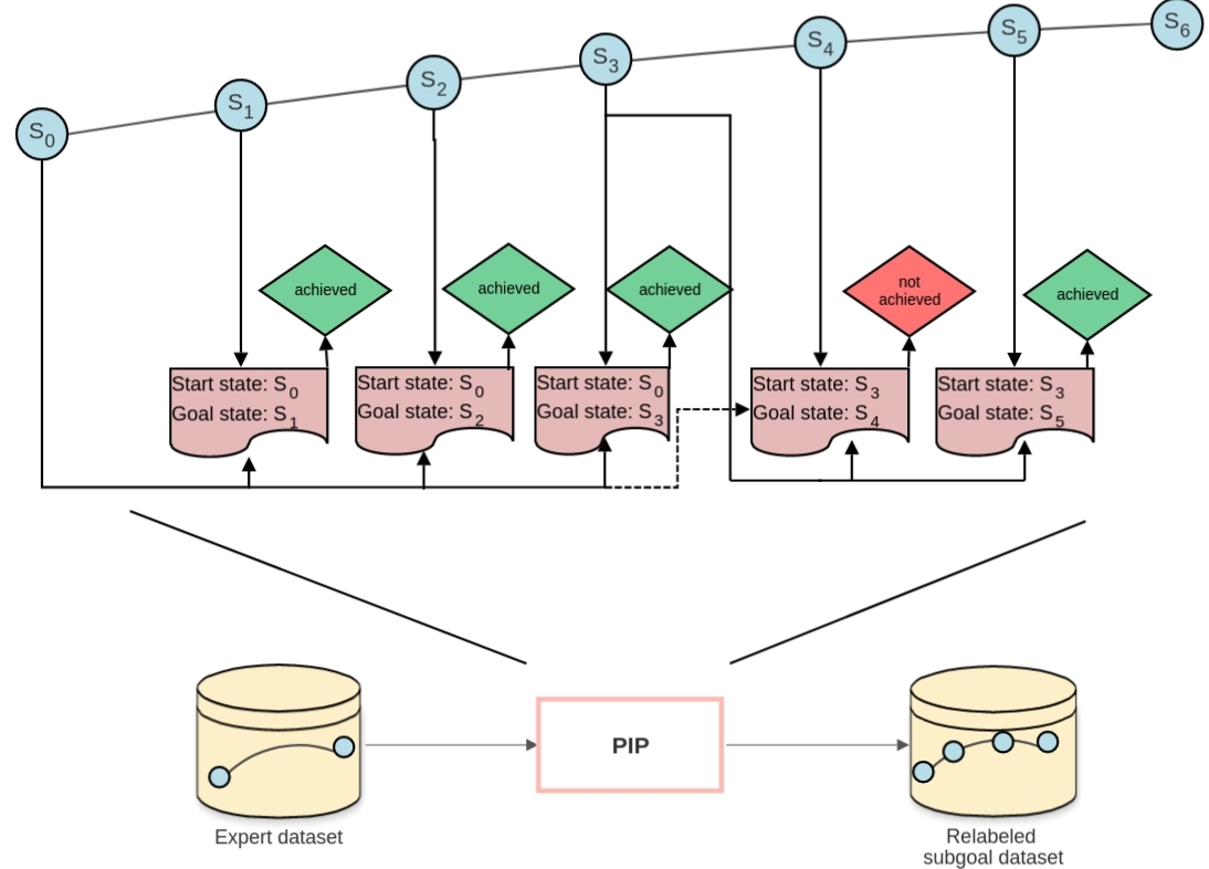
Figure 1: PIP Overview: PIP segments expert demonstrations by consecutively passing demonstration states as subgoals ($s_{i}$: for $i=0$ to $6$). If the lower primitive is unable to achieve state $i$ in $k$ timesteps (here $i=4$), $s_{i-1}$ (here $s_{3}$) is selected as subgoal for initial state $s_{0}$, since $s_{i-1}$ was the last reachable subgoal. The process is repeated with $s_{i-1}$ (here $s_{3}$) as next initial state.

Previous approaches that leverage expert demonstrations have shown impressive results [13, 3, 14]. Expert demonstrations have been used to bootstrap option learning [32, 33, 34, 35]. Other approaches use imitation learning to bootstrap hierarchical approaches in complex task domains [36, 37, 38, 35]. Relay Policy Learning (RPL) [15] uses fixed window based approach for parsing expert demonstrations to generate subgoal transition dataset for training higher level policy. However, fixed parsing based approaches might either predict $(i)$ hard subgoals for the lower level primitive, which impedes the learning progress of lower policy, or $(ii)$ easy subgoals which forces the higher level policy to do most of the heavy-lifting for solving the task. In contrast, our data relabeling technique PIP segments expert demonstration trajectories into meaningful subtasks, which balances the task-split between hierarchical levels. Our adaptive parsing approach considers the limited goal achieving capability of lower primitive, allowing it to produce efficient subgoals.

Prior works employ policy pre-training on related tasks to learn behavior skill priors [39, 40], and then later possibly fine-tuning using RL based approaches. Unfortunately, these approaches fail to generalize when there is distributional shift between initial and target task distributions. Moreover, such approaches may fail to learn a good policy due to sub-optimal expert demonstrations. Other approaches use hand-designed action primitives [41, 42] to encode how to solve sub-tasks, and then to predict $what$ to do by selecting the relevant primitives. It is often tedious to design action primitives, and therefore maintaining sub-task granularity might prove to be burdensome. CRISP side-steps such issues by learning hierarchical policies in parallel, thus allowing the lower policy to learn efficient policies for achieving final goal.

III Background

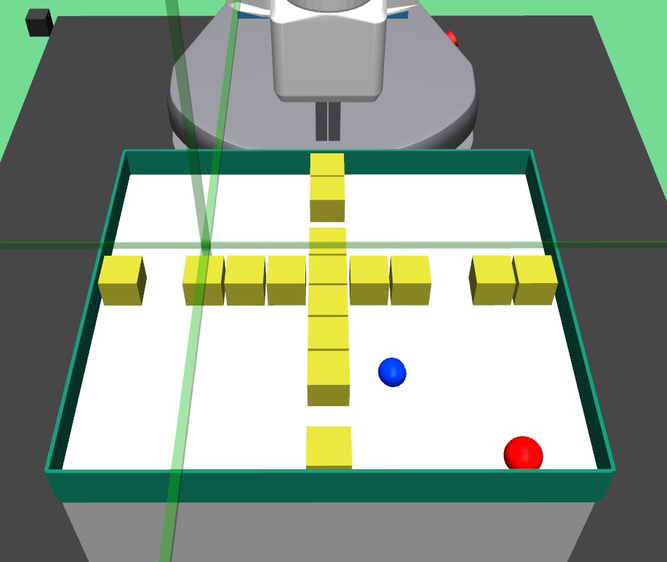
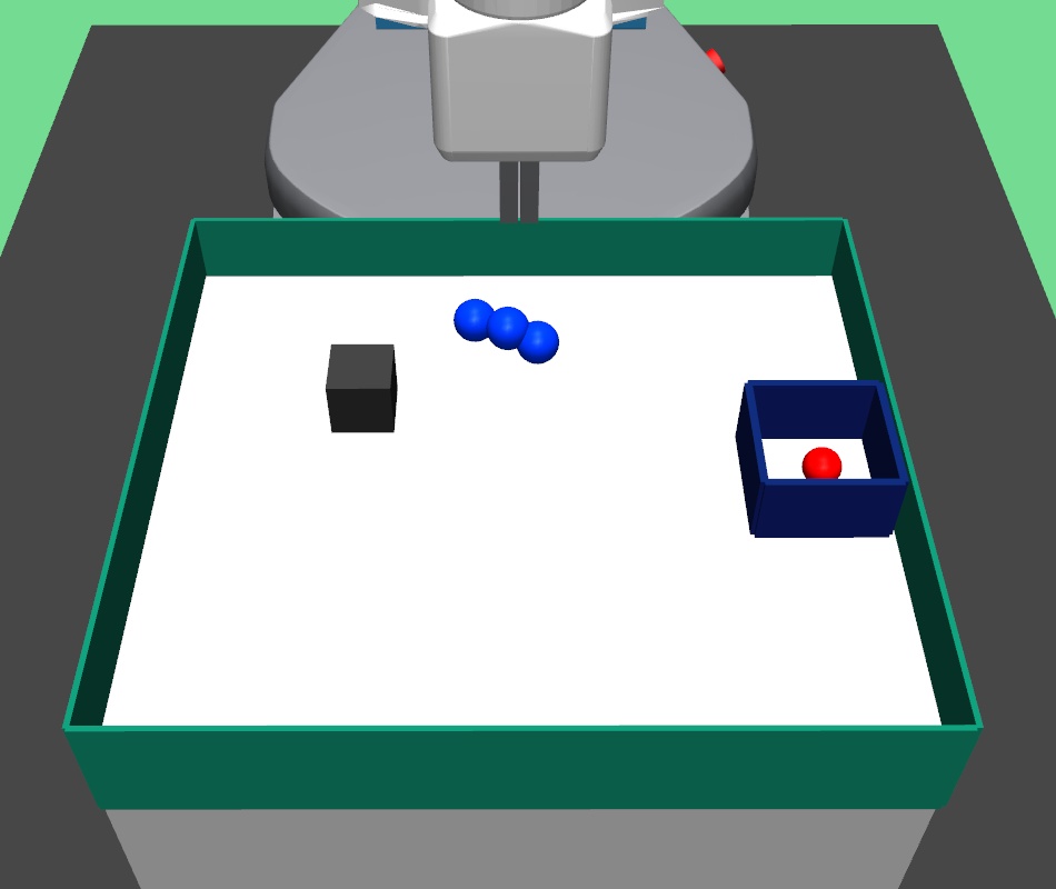
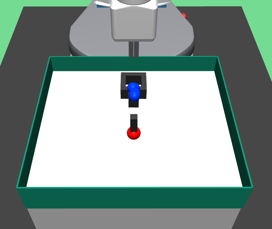
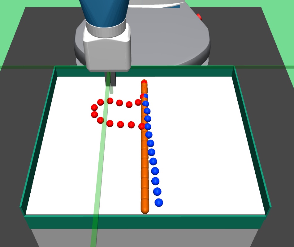
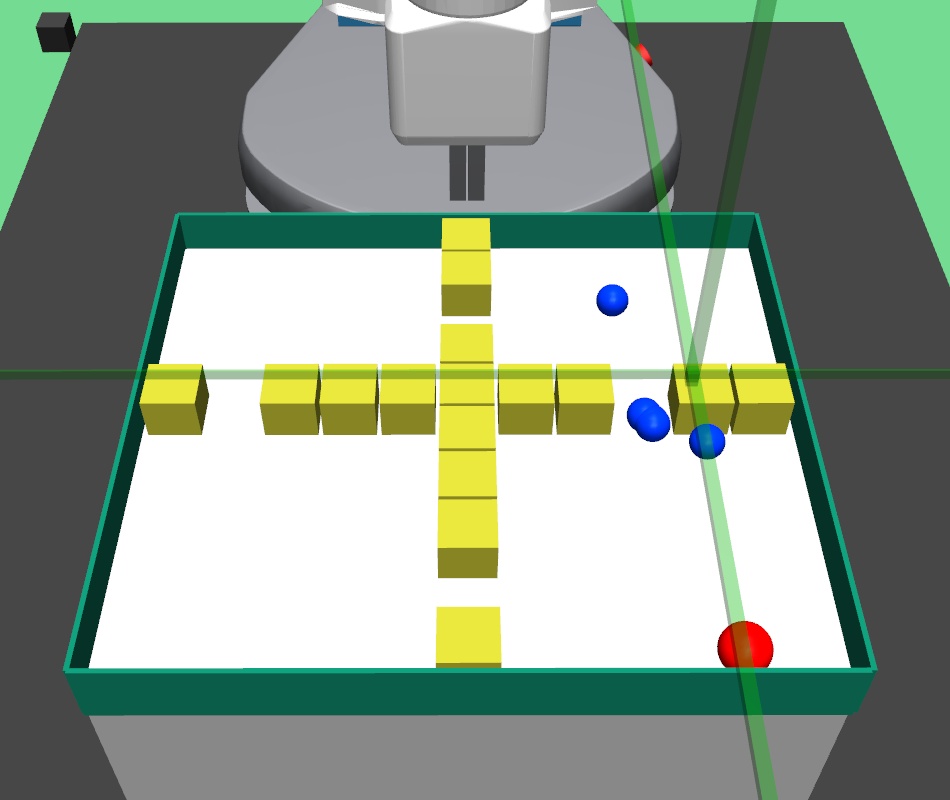
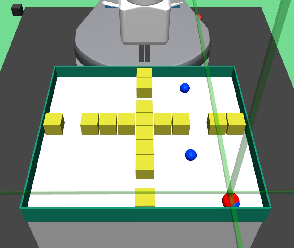
(a)

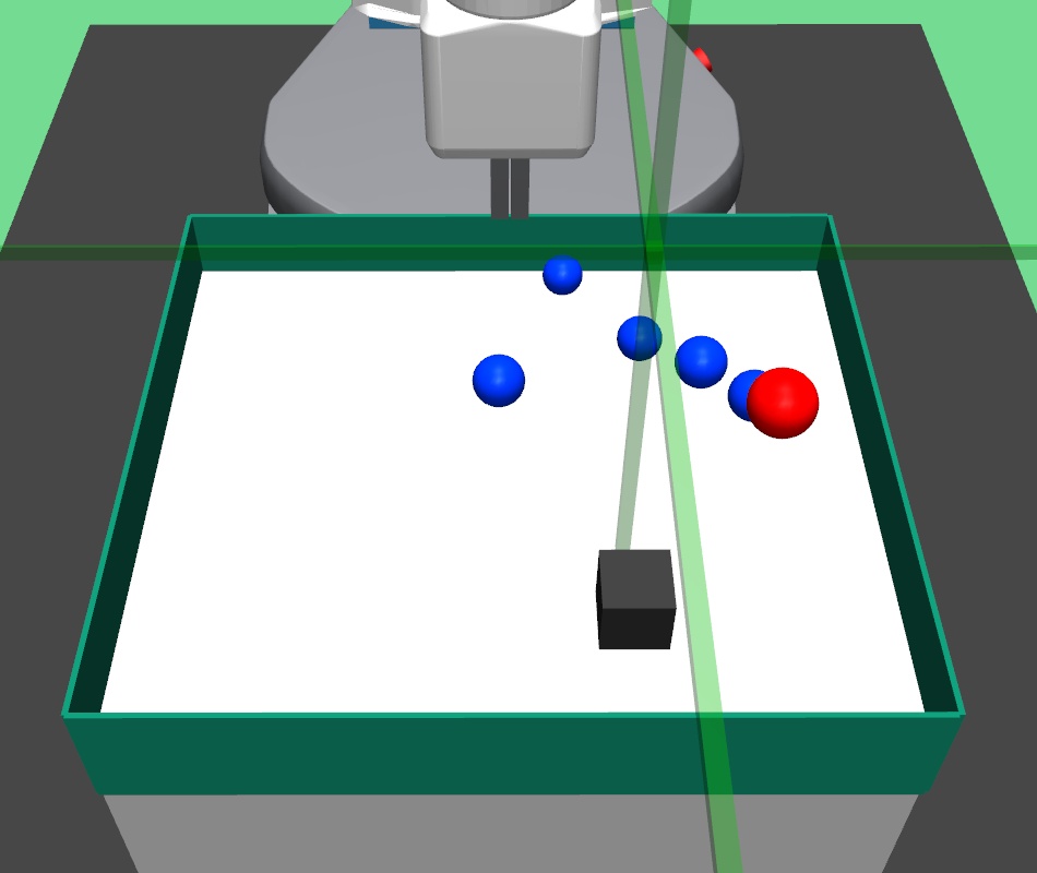
(b)

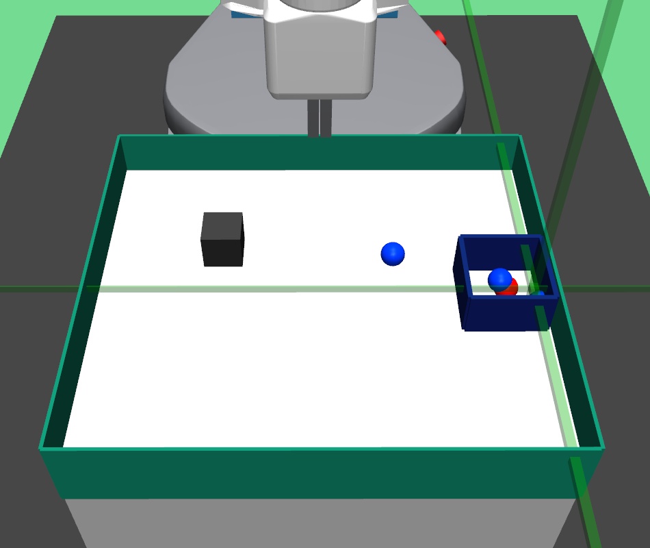
(c)

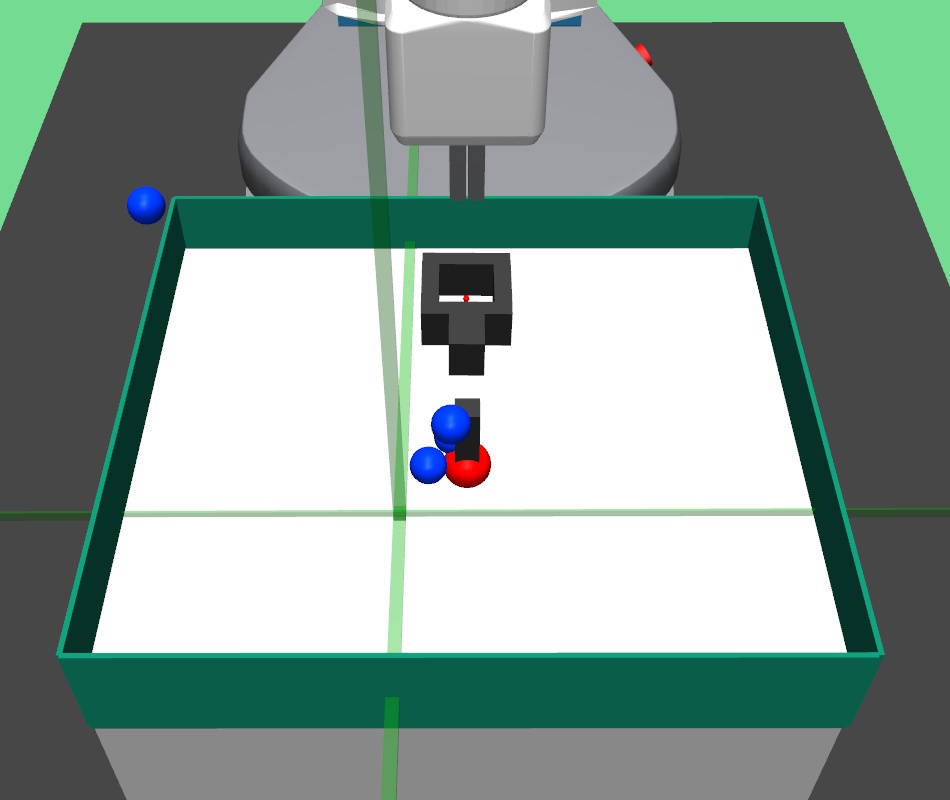
(d)

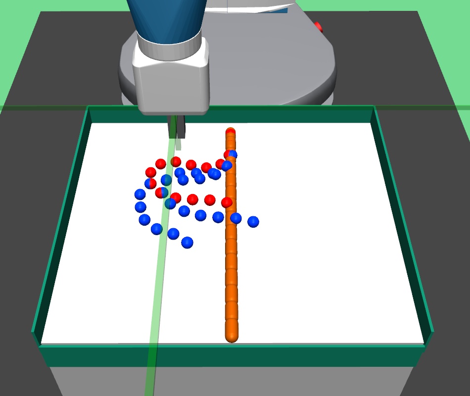
(e)

Figure 2: Subgoal curriculum: This figure depicts the progression of CRISP subgoal generation with training phases (Row 1: initial training, Row 2: mid training, Row 3: end training) in maze navigation, pick and place, bin, hollow, rope and kitchen environment, (walls:yellow, final goal:red, subgoals:blue). CRISP produces a curriculum of reachable subgoals for lower primitive.

We consider Universal Markov Decision Process (UMDP) [43] setting, where Markov Decision processes (MDP) are augmented with the goal space $G$. UMDPs are represented as a 6-tuple $(S,A,P,R,\gamma,G)$, where $S$ is the state space, $A$ is the action space, $P(s^{{}^{\prime}}|s,a)=\mathbb{P}(s_{t+1}=s^{{}^{\prime}}|s_{t}=s,a_{t}=a)$ is the transition function that describes the probability of reaching state $s^{{}^{\prime}}$ when the agent takes action $a$ in the current state $s$. The reward function $R$ generates rewards $r$ at every timestep, $\gamma$ is the discount factor, and $G$ is the goal space. In the UMDP setting, a fixed goal $g$ is selected for an episode, and $\pi(a|s,g)$ denotes the goal-conditioned policy. $d^{\pi}(s)=(1-\gamma)\sum_{t=0}^{T}\gamma^{t}P(s_{t}=s|\pi)$ represents the discounted future state distribution, and $d^{\pi}_{c}(s)=(1-\gamma^{c})\sum_{t=0}^{T}\gamma^{tc}P(s_{tc}=s|\pi)$ represents the c-step future state distribution for policy $\pi$. The overall objective is to learn policy $\pi(a|s,g)$ which maximizes the expected future discounted reward objective $J=(1-\gamma)^{-1}\mathbb{E}_{s\sim d^{\pi},a\sim\pi(a|s,g),g\sim G}\left[r(s_{t},a_{t},g)\right]$

Let $s$ be the current state and $g$ be the final goal for the current episode. In our goal-conditioned hierarchical RL setup, the overall policy $\pi$ is divided into multi-level policies. The higher level policy $\pi^{H}(s_{g}|s,g)$ predicts subgoals [7] $s_{g}$ for the lower level primitive $\pi^{L}(a|s,s_{g})$, which in turn executes primitive actions $a$ directly on the environment. The lower primitive $\pi^{L}$ tries to achieve subgoal $s_{g}$ within $c$ timesteps by maximizing intrinsic rewards $r_{in}$ provided by the higher level policy. The higher level policy $\pi^{H}$ gets extrinsic reward $r_{ex}$ from the environment, and predicts the next subgoal $s_{g}$ for the lower primitive. The process is continued until either the final goal $g$ is achieved, or the episode terminates. We consider sparse reward setting where the lower primitive is sparsely rewarded intrinsic reward $0$ if the agent reaches within $\delta^{L}$ distance of the predicted subgoal $s_{g}$ and $-1$ otherwise: $r_{in}=-1(\|s_{t}-s_{g}\|_{2}>\delta^{L})$, and the higher level policy is sparsely rewarded extrinsic reward $0$ if the achieved goal is within $\delta^{H}$ distance of the final goal $g$, and $-1$ otherwise: $r_{ex}=-1(\|s_{t}-g\|_{2}>\delta^{H})$. We assume access to expert demonstrations $D=\{e^{i}\}_{i=1}^{N}$, where $e^{i}=(s^{e}_{0},s^{e}_{1},\ldots,s^{e}_{T-1})$. We only assume access to demonstration states $s^{e}_{i}$ (and not demonstration actions) which can be obtained in most robotic control tasks.

IV Methodology

Algorithm 1 PIP: Primitive Informed Parsing

Initialize $D_{g}=\{\}$

(final goal) $s_{f}=g$

for each trajectory $e=(s^{e}_{0},s^{e}_{1},\ldots,s^{e}_{T-1})$ in $D$ do

     (initial state) $s_{in}\leftarrow s^{e}_{0}$

     Initialize list of subgoals $D^{e}_{g}=\{\}$

     for i = $1$ to $T-1$ do

         Reset to initial state $s_{in}$

         Pass $s^{e}_{i}$ as the current goal to $\pi_{L}$

         if $s^{e}_{i}$ is not achieved by $\pi_{L}$ in $c$ time-steps then

              Add $(s_{in},s^{e}_{i-1},s_{f})$ to $D^{e}_{g}$

              $s_{in}\leftarrow s^{e}_{i-1}$               

     $D_{g}\leftarrow D_{g}\cup D^{e}_{g}$

In this section, we first explain our primitive informed parsing method PIP, and then explain our hierarchical curriculum learning based approach CRISP. PIP periodically performs data relabeling on expert demonstrations to populate subgoal transition dataset $D_{g}$. We then learn an efficient high level policy by using reinforcement learning and additional inverse reinforcement learning(IRL) based regularization objective.

IV-A Primitive Informed Parsing: PIP

Primitive informed parsing approach uses the current lower primitive $\pi_{L}$ to parse expert state demonstrations dataset $D$. An overview of the method is depicted in Figure 1. We explain below how PIP adaptively parses expert demonstration trajectories from $D$ to generate subgoal transition dataset $D_{g}$.

We start with current lower primitive $\pi_{L}$ and an expert state demonstration trajectory $e=(s^{e}_{0},s^{e}_{1},\ldots,s^{e}_{T-1})$. The environment is reset to initial state $s^{e}_{0}$. Starting at $i=1$ to $T-1$, we incrementally provide states $s^{e}_{i}$ as subgoals to lower primitive $\pi_{L}$. $\pi_{L}$ tries to achieve $s^{e}_{i}$ within $c$ timesteps from the initial state. If $\pi_{L}$ achieves the subgoal $s^{e}_{i}$ within $c$ timesteps, we provide $s^{e}_{i+1}$ as the next subgoal. Conversely, if $\pi_{L}$ fails to achieve the subgoal $s^{e}_{i}$ from the initial state, we add $s^{e}_{i-1}$ to the list of subgoals. The underlying idea is that since $s^{e}_{i-1}$ was the last subgoal achieved by lower-level primitive, it is a good candidate for the next subgoal from initial state. Once we have added $s^{e}_{i-1}$ to the list of subgoals, we continue the process after setting $s^{e}_{i-1}$ as the new initial state until we reach the end of demonstration trajectory $e$. This subgoal transition sequence $D_{g}^{e}$ is added to $D_{g}$. The pseudocode for PIP is given in Algorithm 1. However, PIP assumes ability to reset the environment to any state in $D$. Although this seems impracticable in real world robotic scenarios, this becomes feasible in our setup since we first learn good policies in simulation, and then deploy them in real world. The underlying assumption is that with enough training in simulation, the policy becomes general enough to also perform well in real world. We perform extensive experiments to support this claim in Section V and discuss various ways to relax this assumption in Section VI.

Algorithm 2 CRISP

$D$ (expert demos)

$u$ (population hyperparameter)

Initialize higher level subgoal transition dataset $D_{g}=\{\}$

for epoch $i=1\ldots N$ do

     if $i\%u==0$ then

         Clear $D_{g}$

         Populate $D_{g}$ by relabeling $D$ using PIP      

     for $j$ = $1$ to $T-1$ do

         Collect off policy experience using $\pi_{H}$ and $\pi_{L}$      

     Update lower primitive via SAC and IRL (Eq 4)

     Sample transitions from $D_{g}$

     Update higher policy via SAC and IRL (Eq 3)

IV-B Imitation learning regularization

In this section, we explain how we make use of subgoal transition dataset $D_{g}$ to learn an IRL regularizer. We devise IRL objective as a GAIL [19] like objective implemented using LSGAN [44]. Let $(s^{e},s^{e}_{g},s^{e}_{next})\sim D_{g}$ be higher level subgoal transition from an expert trajectory where $s^{e}$ is current state, $s^{e}_{next}$ is next state, $g^{e}$ is final goal and $s^{e}_{g}$ is subgoal supervision. Let $s_{g}$ be the subgoal predicted by the high level policy $\pi_{\theta_{H}}^{H}(\cdot|s^{e},g^{e})$ with parameters $\theta_{H}$ and $\mathbb{D}_{\epsilon_{H}}^{H}$ be the higher level discriminator with parameters $\epsilon_{H}$. $J_{D}^{H}$ represents upper level IRL objective, which depends on parameters $(\theta_{H},\epsilon_{H})$. We bootstrap the learning of higher level policy by optimizing:

$$\begin{split}&\max_{\theta_{H}}\min_{\epsilon_{H}}J_{D}^{H}(\theta_{H},\epsilon_{H})=\max_{\theta_{H}}\min_{\epsilon_{H}}\frac{1}{2}\mathbb{E}_{(s^{e},s^{e}_{g},\cdot)\sim D_{g}}[\mathbb{D}_{\epsilon_{H}}^{H}(s^{e}_{g})-1]^{2}\\ &\hskip 35.85031pt+\frac{1}{2}\mathbb{E}_{(s^{e},\cdot,\cdot)\sim D_{g},s_{g}\sim\pi_{\theta_{H}}^{H}(\cdot|s^{e},g^{e})}[\mathbb{D}_{\epsilon_{H}}^{H}(\pi_{\theta_{H}}^{H}(\cdot|s^{e},g^{e}))-0]^{2}\end{split}$$ (1)

This objective forces the higher policy subgoal predictions to be close to subgoal predictions of the dataset $D_{g}$. The discriminator $\mathbb{D}_{\epsilon_{H}}^{H}$ creates a natural curriculum for regularizing higher level policy by assigning the value $1$ to the predicted subgoals that are closer to the subgoals from dataset $D_{g}$, and $0$ otherwise. The discriminator improves with training, and regularizes the higher policy to predict achievable subgoals.

Similarly for lower level primitive, let $(s^{f},a^{f},s^{f}_{next})\sim D_{g}^{L}$ be lower level expert transition where $s^{f}$ is current state, $s^{f}_{next}$ is next state, $g^{f}$ is final goal, $a$ is the primitive action predicted by lower policy $\pi_{\theta_{L}}^{L}(\cdot|s^{f},s^{e}_{g})$ with parameters $\theta_{L}$, and $\mathbb{D}_{\epsilon_{L}}^{L}$ be the lower level discriminator with parameters $\epsilon_{L}$. Let $J_{D}^{L}$ represent lower level IRL objective, which depends on parameters $(\theta_{L},\epsilon_{L})$. The lower level IRL objective is thus:

$$\begin{split}&\max_{\theta_{L}}\min_{\epsilon_{L}}J_{D}^{L}(\theta_{L},\epsilon_{L})=\max_{\theta_{L}}\min_{\epsilon_{L}}\frac{1}{2}\mathbb{E}_{(s^{f},a^{f},\cdot)\sim D_{g}^{L}}[\mathbb{D}_{\epsilon_{L}}^{L}(a^{f})-1]^{2}\\ &\hskip 38.12659pt+\frac{1}{2}\mathbb{E}_{(s^{f},\cdot,\cdot)\sim D_{g}^{L},a\sim\pi_{\theta_{L}}^{L}(\cdot|s^{f},s^{e}_{g})}[\mathbb{D}_{\epsilon_{L}}^{L}(\pi_{\theta_{L}}^{L}(\cdot|s^{f},s^{e}_{g}))-0]^{2}\end{split}$$ (2)

IV-C Joint optimization

The higher level policy is trained to produce subgoals, which when fed into the lower level primitive, maximize the sum of future discounted rewards for our task using off-policy reinforcement learning. Here $T$ is the task horizon and $g$ is the sampled goal for the current episode. For brevity, we can refer to this objective function as $J^{H}_{\theta_{H}}$ and $J^{L}_{\theta_{L}}$ for upper and lower level policies. We use the IRL objective to regularize the high level off-policy RL objective as follows:

$$\max_{\theta_{H}}(J^{H}_{\theta_{H}}+\psi*(\min_{\epsilon_{H}}J_{D}^{H}(\theta_{H},\epsilon_{H})))$$ (3)

whereas the lower level primitive is trained by optimizing:

$$\max_{\theta_{L}}(J^{L}_{\theta_{L}}+\psi*(\min_{\epsilon_{L}}J_{D}^{L}(\theta_{L},\epsilon_{L})))$$ (4)

The lower policy is regularized using expert demonstration dataset, and the upper level is optimized using subgoal transition dataset populated using PIP. $\psi$ is the regularization weight hyper-parameter for the IRL objective. When $\psi=0$, the method reduces to HRL policy with no higher level policy regularization. When $\psi$ is too high, the method might overfit to the expert demonstration dataset. We perform ablation analysis to choose $\psi$ in Appendix Section VII-C. The CRISP algorithm is shown in Algorithm 2.

V Experiments

In this section, we perform experimental analysis to answer whether: $(i)$ adaptive relabeling using PIP outperforms fixed window parsing approaches, $(ii)$ CRISP predicts better subgoals using imitation learning regularization, and $(iii)$ hierarchical curriculum learning mitigates non-stationarity issue. Along with IRL regularization, we also use behavior cloning (BC) regularization for regularizing the higher policy. In BC regularization for regularizing the higher policy, the IRL objective is replaced by BC objective. Henceforth, CRISP-IRL will denote CRISP with IRL regularization, and CRISP-BC will denote CRISP with BC regularization. We perform experiments on six complex robotic environments with continuous state and action spaces that require long term planning: $(i)$ maze navigation, $(ii)$ pick and place, $(iii)$ bin, $(iv)$ hollow, $(v)$ rope manipulation, and $(vi)$ franka kitchen. We empirically compare our approach with various baselines in Table I. For qualitative results, please refer to the supplementary video https://tinyurl.com/crispVideo.

V-A Environment Setup

The simulation environments designed in Mujoco[45] are sparse reward environments where the agent only gets a reward if it achieves the final goal. The robotic maze navigation, pick and place, bin, hollow and rope environments employ a $7$-DOF robotic arm gripper whereas the kitchen environment employs a $9$-DoF franka robot gripper. In the maze navigation task, the gripper (whose height is kept fixed at table height) has to navigate across randomly generated four room mazes (the wall and gate positions are randomly generated) to achieve final goal. In the pick and place task, the gripper has to pick a randomly placed square block and bring it to a randomly generated goal position. In bin environment, the gripper has to pick up the block and place it in a specific bin. In the hollow task, the gripper has to pick a square hollow block and place it across a fixed vertical pole on the table such that the block goes through the pole. In rope manipulation task, a deformable soft rope is kept on the table and the gripper performs pokes on the rope to nudge it towards the goal rope configuration. The rope manipulation task involves learning challenging dynamics and goes beyond prior work on navigation-like tasks where the goal space is limited. In kitchen task, the gripper has to first open the microwave door, and then switch on the specific gas knob where the kettle is placed.

TABLE I: Success rate comparison

	Maze	Pick Place	Bin	Hollow	Rope	Kitchen
CRISP-IRL (ours)	0.81 $\pm$ 0.03	0.93 $\pm$ 0.03	0.77 $\pm$ 0.04	1.0 $\pm$ 0.0	0.21 $\pm$ 0.01	0.7 $\pm$ 0.06
CRISP-BC (ours)	0.51 $\pm$ 0.01	0.77 $\pm$ 0.08	0.55 $\pm$ 0.17	0.98 $\pm$ 0.03	0.34 $\pm$ 0.06	0.31 $\pm$ 0.1
RPL	0.58 $\pm$ 0.09	0.28 $\pm$ 0.17	0.0 $\pm$ 0.0	0.0 $\pm$ 0.0	0.13 $\pm$ 0.07	0.08 $\pm$ 0.1
HAC	0.6 $\pm$ 0.23	0.0 $\pm$ 0.0	0.0 $\pm$ 0.0	0.1 $\pm$ 0.0	0.02 $\pm$ 0.01	0.0 $\pm$ 0.0
RAPS	0.81 $\pm$ 0.06	0.0 $\pm$ 0.0	0.0 $\pm$ 0.0	0.0 $\pm$ 0.0	-	0.0 $\pm$ 0.0
HIER-NEG	0.01 $\pm$ 0.0	0.0 $\pm$ 0.0	0.0 $\pm$ 0.0	0.0 $\pm$ 0.0	0.01 $\pm$ 0.0	0.0 $\pm$ 0.0
HIER	0.02 $\pm$ 0.02	0.0 $\pm$ 0.0	0.0 $\pm$ 0.0	0.0 $\pm$ 0.0	0.01 $\pm$ 0.0	0.0 $\pm$ 0.0
DAC	0.02 $\pm$ 0.02	0.21 $\pm$ 0.06	0.14 $\pm$ 0.09	0.0 $\pm$ 0.0	0.03 $\pm$ 0.01	0.0 $\pm$ 0.0
FLAT	0.01 $\pm$ 0.01	0.0 $\pm$ 0.0	0.0 $\pm$ 0.0	0.0 $\pm$ 0.0	0.03 $\pm$ 0.01	0.0 $\pm$ 0.0
BC	0.0	0.0	0.0	0.0	0.15	0.0

(a)

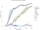
(b)

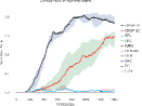
(c)

(d)

(e)

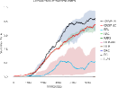
(f)

Figure 3: Success rate comparison in maze, pick and place, bin, hollow, rope, and kitchen tasks vs number of timesteps.

V-B Implementation details

In our experiments, the regularization weight hyper-parameter $\Psi$ is set to $0.001$, $0.005$, $0.005$, $0.005$, $0.005$, and $0.005$ and population hyper-parameter $p$ is set to be $1.1e4$, $2500$, $2500$, $2500$, $3.9e5$, and $1.4e4$ for maze, pick and place, bin, hollow, rope and kitchen respectively. We use off-policy Soft Actor Critic [46] RL objective with Adam [47] optimizer. The hand designed action primitives from RAPS [41] are designed as follows: $(i)$ in maze navigation, the lower level primitive travels in a straight line directly towards the subgoal $(x_{i},y_{i},z_{i})$ predicted by higher level policy, $(ii)$ in pick and place, bin and hollow tasks, we hand-designed three primitives: gripper-reach (where the gripper has to reach the position $(x_{i},y_{i},z_{i})$), gripper-open (where the robotic arm has to open the gripper) and gripper-close (where the robotic arm has to close the gripper). In kitchen environment, we use the action primitives implemented in RAPS [41]. Since it is hard to design the action primitives in rope environment, we do not evaluate RAPS in the environment. The maximum task horizon $T$ is kept at $225$, $50$, $60$, $100$ $25$, and $280$ timesteps, the lower primitive is allowed to execute for $15$, $7$, $6$, $10$, $5$, and $17$ timesteps, and the experiments are run for $c$ $4.73e5$, $1.1e5$, $1.32E5$, $3.5E5$, $1.58e6$, and $5.32e5$ timesteps in maze, pick and place, bin, hollow, rope and kitchen tasks respectively. For collecting expert demonstrations, we use RRT [48] based trajectories in maze task, Mujoco VR [49] based direction in pick and place, bin and hollow tasks, poking based expert controller in rope task, and D4RL [50] expert data in kitchen task. We provide more environments details and detailed expert demonstrations collection procedures for all tasks in Appendix Section VII-A and Section VII-B respectively.

V-C Comparative analysis

In Table I, we compare the success rate performances of CRISP with various hierarchical and non-hierarchical baselines. The performances are averaged over $5$ seeds and evaluated over $100$ rollouts. As explained in Section IV, CRISP-IRL uses IRL and CRISP-BC uses BC regularization. As shown in Table I, CRISP-IRL and CRISP-BC are consistently outperform other baselines in all tasks. RPL (Relay Policy Learning) [15] is a fixed window based approach that first uses supervised pre-training from undirected demonstrations, and then fine-tunes the policy using RL. We use a variant of RPL which does not use this pre-training to ascertain fair comparisons. Our method outperforms RPL in all tasks, which demonstrates that adaptive relabeling is able to select better subgoals, which are subsequently used to regularize the higher level policy. Notably, to elucidate the importance of adaptive relabeling, we also consider a variant of our method which uses IRL regularization with fixed window based relabeling. We compare this variant (CRISP-RPL) with our approach in Section V-E. Our method outperforms this baseline, showing shows that both adaptive relabeling and IRL regularization are crucial for solving complex tasks.

Hierarchical Actor Critic (HAC) [12] is a hierarchical approach that deals with the non-stationarity issue by appending replay buffer with additional transitions which consider an optimal lower level policy. As seen in Table I, although HAC performs well in easier tasks, it is unable to perform well when task complexity increases. Our method outperforms HAC, which shows that hierarchical curriculum learning shows impressive results when dealing with non-stationarity issue. In recent work like RAPS [41], hand-designed action primitives are used to predict primitive actions. The upper level then has to pick from among these action primitives, thereby abstracting the ”how” from the ”what” in the given task. However, the performance of such approaches depends on the quality of the primitives, and the feasibility of designing action primitives. RAPS performs exceptionally well in maze navigation since the hand-designed action primitive is approximately optimal. However, it fails to perform well in other complex environments, possibly because either the task is too complex or the hand-designed action primitives are sub-optimal. In rope manipulation environment, designing the action primitives is hard. In contrast, our method trains multiple levels in parallel, which allows the lower level primitives to be approximately optimal policies.

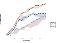
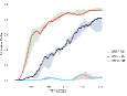
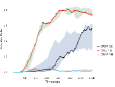
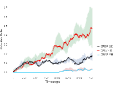
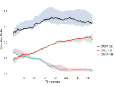
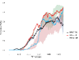
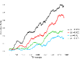
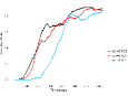
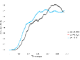
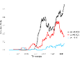
(a)

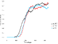
(b)

(c)

(d)

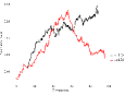
(e)

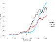
(f)

Figure 4: Ablation experiments in various environments: $(i)$ Row 1: CRISP vs CRISP-RPL performance comparison, $(ii)$ Row 2: learning rate, and $(iii)$ Row 3: $p$ hyperparameter.

(a)

(b)

(c)

Figure 5: Real world experiments in pick and place, bin and rope manipulation tasks. Row 1 depicts initial and Row 2 depicts final goal configuration.

We also compare our approach with two other hierarchical baselines: HIER and HIER-NEG, which are hierarchical off-policy SAC based baselines that do not leverage expert demonstrations. Additionally, in HIER-NEG the higher level policy is negatively rewarded if the lower primitive is unable to reach the predicted subgoal. Both these policies fail to perform well in any of the tasks. We also compare our approach with two flat single-level policies: Discriminator actor critic (DAC), and a single level SAC policy FLAT and show that our hierarchical curriculum learning approach is crucial for good performance. We also compare our approach with behavior cloning (BC) baseline and demonstrate that RL and IL regularization are crucial for improved performance and sample complexity. We report the success rate comparison plots in Figure 3. In all tasks, our method consistently outperforms the baselines and demonstrates faster convergence.

V-D Real world experiments

In order to qualitatively analyse whether the learnt policies can be deployed in real world robotic tasks, we perform real robotic experiments in pick and place, bin and rope manipulation environments (Fig 5). CRISP-IRL achieves an accuracy of $0.6$, $0.6$ and $0.1$, whereas CRISP-BC achieved accuracy of $0.8$, $0.3$, $0.2$ on pick and place, bin and rope environments respectively. We also deployed the next best performing baseline RPL on the four tasks, but it was unable to achieve the goal in any of the tasks.

V-E Ablative studies

Finally, we perform ablation analysis to elucidate the significance of various design choices in our proposed approach. CRISP uses adaptive relabeling to generate efficient subgoal supervision, and subsequently uses imitation learning regularization for efficiently training hierarchical levels. In order to demonstrate the importance of adaptive relabeling, we replace adaptive relabeling in CRISP-IRL with fixed window relabeling like RPL [15]. We call the ablation CRISP-RPL and compare the performance with CRISP-IRL and CRISP-BC in Figure 4 Row 1. In almost all the environments, our method outperforms this baseline, thus empirically verifying that adaptive relabeling is crucial for improved performance, stable learning and better sample efficiency. We also perform ablations to select the hyperparameters $(i)$ learning rate $\psi$ (Figure 4 Row 2), and population hyperparameter $p$ (Figure 4 Row 3). When $\psi$ is too high, the method might overfit to the expert demonstrations. We empirically found that large values of $p$ are unable to generate good curriculum of subgoals.

We also perform ablations to deduce the optimal number of expert demonstrations required for each task. We use $28$ expert demonstrations in kitchen and $100$ in other tasks. If the number of expert data is too small, the policy may overfit to the limited data. Although the number of expert demonstrations are subject to availability, we increase the number until there is no significant improvement in performance. We also empirically analyse the effect of varying the quality of expert data. We found direct co-relation between the quality of expert data and overall performance. In future work, we plan to make CRISP more robust towards bad demonstrations. Furthermore, we empirically choose the best value of window size hyper-parameter $k$ in all tasks. We provide these ablation experiments and qualitative visualizations for all tasks in simulation in Appendix Sections VII-C and VII-D.

VI Conclusion

Limitations: In our approach, we perform periodic adaptive relabeling, which is an additional overhead especially in long-horizon tasks where relabeling cost is high. Since we train our policies in simulation and deploy on real robotic environments, we empirically found this to be a marginal overhead. Nonetheless, we plan to devise methods to remove this limitation in future work. Our method assumes availability of a handful of directed expert demonstrations. It would be interesting to analyze the performance of our method when the demonstrations are undirected. In future work, we plan to devise methods that work well in such scenarios. Additionally, CRISP assumes the ability to reset the environment to any state from expert demonstrations while collecting subgoal dataset using PIP. A possible method for relaxing this assumption is to combine CRISP with [51] that learns a backward controller that tries to reset the environment. We believe that this is an interesting avenue for future work.

Discussion and future work: We introduce CRISP, a general purpose primitive informed method for efficient curriculum based hierarchical reinforcement learning. CRISP leverages primitive parsed expert demonstrations and performs adaptive data relabeling to populate subgoal transition dataset for regularizing higher level policy. Furthermore, CRISP employs hierarchical curriculum learning for solving complex tasks requiring long term planning. We evaluate our method on complex robotic navigation and manipulation tasks in simulation, deploy them in real world scenarios, and demonstrate that our approach shows substantial gains over its baselines. We hope that this work encourages future work in adaptive relabeling and hierarchical curriculum learning.

VII Appendix

VII-A Environment details

In this subsection, we provide the environment and implementation details for all the tasks:

VII-A1 Maze navigation task

In this environment, a $7$-DOF robotic arm gripper navigates across random four room mazes to reach the goal position. The gripper arm is kept closed and fixed at table height, and the positions of walls and gates are randomly generated. The table is discretized into a rectangular $W*H$ grid, and the vertical and horizontal wall positions $W_{P}$ and $H_{P}$ are randomly picked from $(1,W-2)$ and $(1,H-2)$ respectively. In the four room environment thus constructed, the four gate positions are randomly picked from $(1,W_{P}-1)$, $(W_{P}+1,W-2)$, $(1,H_{P}-1)$ and $(H_{P}+1,H-2)$.

In the maze environment, the state is represented as the vector $[x,M]$, where $x$ is current gripper position and $M$ is the sparse maze array. The higher level policy input is thus a concatenated vector $[x,M,g]$, where $g$ is the target goal position, whereas the lower level policy input is concatenated vector $[x,M,s_{g}]$, where $s_{g}$ is the sub-goal provided by the higher level policy. $M$ is a discrete $2D$ one-hot vector array, where $1$ represents presence of a wall block, and otherwise. The lower primitive action $a$ is a $4$ dimensional vector with every dimension $a_{i}\in[0,1]$. The first $3$ dimensions provide offsets to be scaled and added to gripper position for moving it to the intended position. The last dimension provides gripper control($0$ implies a closed gripper and $1$ implies an open gripper). We select $100$ randomly generated mazes each for training, testing and validation.

VII-A2 Pick and place, bin and hollow environments

In this subsection, we explain the environment details for the pick and place, bin and hollow tasks. The state is represented as the vector $[x,o,q,e]$, where $x$ is the current gripper position, $o$ is the position of the block object placed on the table, $q$ is the relative position of the block with respect to the gripper, and $e$ consists of linear and angular velocities of the gripper and the block object. The higher level policy input is thus a concatenated vector $[x,o,q,e,g]$, where $g$ is the target goal position. The lower level policy input is concatenated vector $[x,o,q,e,s_{g}]$, where $s_{g}$ is the sub-goal provided by the higher level policy. In our experiments, we keep the sizes of $x$, $o$, $q$, $e$ to be $3$, $3$, $3$ and $11$ respectively. The lower primitive action $a$ is a $4$ dimensional vector with every dimension $a_{i}\in[0,1]$. The first $3$ dimensions provide gripper position offsets, and the last dimension provides gripper control. While training, the position of block object and goal are randomly generated (block is always initialized on the table, and goal is always above the table at a fixed height). We select $100$ random each for training, testing and validation.

VII-A3 Rope Manipulation Environment

In this environment, the deformable rope is formed from $15$ constituent cylinders joined together. The state space for the rope manipulation environment is a vector formed by concatenation of the intermediate joint positions. The upper level predicts subgoal $s_{g}$ for the lower primitive. The action space of the poke is $(x,y,\eta)$, where $(x,y)$ is the initial position of the poke, and $\eta$ is the angle describing the direction of the poke. We fix the poke length to be $0.08$. We select $100$ randomly generated initial and final rope configurations each for training, testing and validation.

VII-A4 Franka kitchen Environment

For this environment please refer to the D4RL environment [\cite[cite]{[\@@bibref{}{DBLP:journals/corr/abs-2004-07219}{}{}]}]. In this environment, the franka robot has to perform a complex multi-stage task in order to achieve the final goal.

VII-B Generating expert demonstrations

We explain the procedure for geenrating expert demonstrations as follows:

VII-B1 Maze navigation Environment

We use the path planning RRT [52] algorithm to generate optimal paths $P=(p_{t},p_{t+1},p_{t+2},...p_{n})$ from the initial state to the goal state. Using these expert paths, we generate state-action expert demonstration dataset for the lower level policy, which is later used to generate subgoal transition dataset. Since the procedure is automated using RRT algorithm, we can generate expert demonstrations without the expert.

VII-B2 Pick and place Environment

For generating expert demonstrations, we initially used a human agent in virtual reality based Mujoco simulation to generate demonstrations. We later found that hard coding a control policy also works reasonably well in this environment. Hence, we used a hard-coded policy to generate the expert demonstrations. In this task, the robot firstly picks up the block using robotic gripper, and then takes it to the target goal position.

VII-B3 Bin Environment

In this environment, we used a hard-coded policy to generate the expert demonstrations. In this task, the robot firstly picks up the block using robotic gripper, and then places it in the target bin. Using these expert trajectories, we generate expert demonstration dataset for the lower level policy.

VII-B4 Hollow Environment

In this environment, we used a hard-coded policy to generate the expert demonstrations. In this task, the robotic gripper has to pick up the square hollow block and place it such that a vertical structure on the table goes through the hollow block.

VII-B5 Rope Manipulation Environment

We hand coded an expert policy to automatically generate expert demonstrations $e=(s^{e}_{0},s^{e}_{1},\ldots,s^{e}_{T-1})$, where $s^{e}_{i}$ are demonstration states. The states $s^{e}_{i}$ here are rope configuration vectors. The expert policy is explained below.

Let the starting and goal rope configurations be $sc$ and $gc$. We find the cylinder position pair $(sc_{m},gc_{m})$ where $m\in[1,n]$, such that $sc_{m}$ and $gc_{m}$ are farthest from each other among all other cylinder pairs. Then, we perform a poke $(x,y,\theta)$ to drag $sc_{m}$ towards $gc_{m}$. The $(x,y)$ position of the poke is kept close to $sc_{m}$, and poke direction $\theta$ is the direction from $sc_{m}$ towards $gc_{m}$. After the poke execution, the next pair of farthest cylinder pair is again selected and another poke is executed. This is repeatedly done for $k$ pokes, until either the rope configuration $sc$ comes within $\delta$ distance of goal $gc$, or we reach maximum episode horizon $T$. Although, this policy is not the perfect policy for goal based rope manipulation, but it still is a good expert policy for collecting demonstrations $D$. Moreover, as our method requires states and not primitive actions (pokes), we can use these demonstrations $D$ to collect good higher level subgoal dataset $D_{g}$ using primitive parsing.

VII-B6 Kitchen Environment

In this environment, we used the expert demonstrations provided in D4RL dataset[50]. We use directed demonstrations from this dataset to solve the multi-stage task in this environment.

VII-C Ablation experiments

In this subsection we provide the ablation experiments in all six task environments. The ablation analysis includes performance comparison of RPL window size hyperparameter (Figure 6), and comparisons with varying number of expert demonstrations (Figure 7) used during relabeling and training.

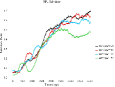
(a)

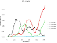
(b)

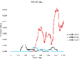
(c)

(d)

(e)

(f)

Figure 6: Column 1-6 depict ablation experiments for window size hyper-parameter in RPL experiments.

(a)

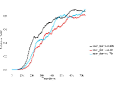
(b)

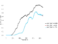
(c)

(d)

(e)

(f)

Figure 7: Column 1-6 depict ablation experiments of varying number of expert demonstrations versus number of training epochs.

VII-D Qualitative visualizations

In this subsection, we provide visualization of successful and failure cases for some of the testing runs in various environments:

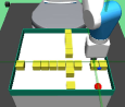
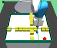
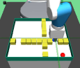
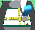
Figure 8: Successful visualization: The visualization is a successful attempt at performing maze navigation task

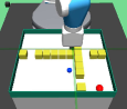
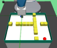
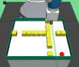
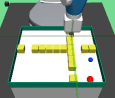
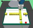
Figure 9: Failed visualization: The visualization is a failed attempt at performing maze navigation task

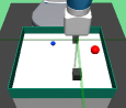
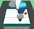
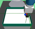
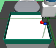
Figure 10: Successful visualization: The visualization is a successful attempt at performing pick navigation task

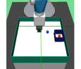
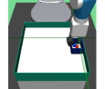
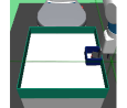
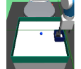
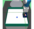
Figure 11: Successful visualization: The visualization is a successful attempt at performing bin task

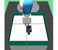
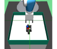
Figure 12: Successful visualization: The visualization is a successful attempt at performing hollow task

Figure 13: Failed visualization: The visualization is a failed attempt at performing hollow task

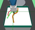
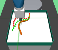
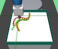
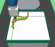
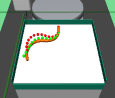
Figure 14: Successful visualization: The visualization is a successful attempt at performing rope navigation task

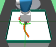
Figure 15: Failed visualization: The visualization is a failed attempt at performing rope navigation task

Figure 16: Successful visualization: The visualization is a successful attempt at performing kitchen navigation task

Figure 17: Failed visualization: The visualization is a failed attempt at performing kitchen navigation task

References

- [1] S. Levine, C. Finn, T. Darrell, and P. Abbeel, “End-to-end training of deep visuomotor policies,” CoRR, vol. abs/1504.00702, 2015.
- [2] M. Vecerík, T. Hester, J. Scholz, F. Wang, O. Pietquin, B. Piot, N. Heess, T. Rothörl, T. Lampe, and M. A. Riedmiller, “Leveraging demonstrations for deep reinforcement learning on robotics problems with sparse rewards,” CoRR, vol. abs/1707.08817, 2017.
- [3] A. Rajeswaran, V. Kumar, A. Gupta, J. Schulman, E. Todorov, and S. Levine, “Learning complex dexterous manipulation with deep reinforcement learning and demonstrations,” CoRR, vol. abs/1709.10087, 2017.
- [4] O. Nachum, H. Tang, X. Lu, S. Gu, H. Lee, and S. Levine, “Why does hierarchy (sometimes) work so well in reinforcement learning?” arXiv preprint arXiv:1909.10618, 2019.
- [5] T. D. Kulkarni, K. Narasimhan, A. Saeedi, and J. B. Tenenbaum, “Hierarchical deep reinforcement learning: Integrating temporal abstraction and intrinsic motivation,” CoRR, vol. abs/1604.06057, 2016.
- [6] M. Andrychowicz, F. Wolski, A. Ray, J. Schneider, R. H. Fong, P. Welinder, B. McGrew, J. Tobin, P. Abbeel, and W. Zaremba, “Hindsight experience replay,” in NIPS, 2017.
- [7] P. Dayan and G. E. Hinton, “Feudal reinforcement learning,” in Advances in Neural Information Processing Systems 5, [NIPS Conference]. San Francisco, CA, USA: Morgan Kaufmann Publishers Inc., 1993, pp. 271–278.
- [8] R. S. Sutton, D. Precup, and S. Singh, “Between mdps and semi-mdps: A framework for temporal abstraction in reinforcement learning,” Artificial Intelligence, vol. 112, no. 1, pp. 181–211, 1999. [Online]. Available: https://www.sciencedirect.com/science/article/pii/S0004370299000521
- [9] R. Parr and S. Russell, “Reinforcement learning with hierarchies of machines,” in Advances in Neural Information Processing Systems, M. Jordan, M. Kearns, and S. Solla, Eds., vol. 10. MIT Press, 1998.
- [10] O. Nachum, S. Gu, H. Lee, and S. Levine, “Data-efficient hierarchical reinforcement learning,” CoRR, vol. abs/1805.08296, 2018.
- [11] A. S. Vezhnevets, S. Osindero, T. Schaul, N. Heess, M. Jaderberg, D. Silver, and K. Kavukcuoglu, “Feudal networks for hierarchical reinforcement learning,” CoRR, vol. abs/1703.01161, 2017.
- [12] A. Levy, R. P. Jr., and K. Saenko, “Hierarchical actor-critic,” CoRR, vol. abs/1712.00948, 2017.
- [13] A. Nair, B. McGrew, M. Andrychowicz, W. Zaremba, and P. Abbeel, “Overcoming exploration in reinforcement learning with demonstrations,” CoRR, vol. abs/1709.10089, 2017.
- [14] T. Hester, M. Vecerík, O. Pietquin, M. Lanctot, T. Schaul, B. Piot, A. Sendonaris, G. Dulac-Arnold, I. Osband, J. P. Agapiou, J. Z. Leibo, and A. Gruslys, “Learning from demonstrations for real world reinforcement learning,” CoRR, vol. abs/1704.03732, 2017.
- [15] A. Gupta, V. Kumar, C. Lynch, S. Levine, and K. Hausman, “Relay policy learning: Solving long-horizon tasks via imitation and reinforcement learning,” CoRR, vol. abs/1910.11956, 2019.
- [16] Y. Bengio, J. Louradour, R. Collobert, and J. Weston, “Curriculum learning,” in Proceedings of the 26th Annual International Conference on Machine Learning, ser. ICML ’09. New York, NY, USA: Association for Computing Machinery, 2009, p. 41–48. [Online]. Available: https://doi.org/10.1145/1553374.1553380
- [17] S. K. S. Ghasemipour, R. Zemel, and S. Gu, “A divergence minimization perspective on imitation learning methods,” in Conference on Robot Learning. PMLR, 2020, pp. 1259–1277.
- [18] I. Kostrikov, K. K. Agrawal, D. Dwibedi, S. Levine, and J. Tompson, “Discriminator-actor-critic: Addressing sample inefficiency and reward bias in adversarial imitation learning,” arXiv preprint arXiv:1809.02925, 2018.
- [19] J. Ho and S. Ermon, “Generative adversarial imitation learning,” CoRR, vol. abs/1606.03476, 2016. [Online]. Available: http://arxiv.org/abs/1606.03476
- [20] A. G. Barto and S. Mahadevan, “Recent advances in hierarchical reinforcement learning,” Discrete Event Dynamic Systems, vol. 13, pp. 341–379, 2003.
- [21] T. G. Dietterich, “Hierarchical reinforcement learning with the MAXQ value function decomposition,” CoRR, vol. cs.LG/9905014, 1999. [Online]. Available: https://arxiv.org/abs/cs/9905014
- [22] P. Bacon, J. Harb, and D. Precup, “The option-critic architecture,” CoRR, vol. abs/1609.05140, 2016.
- [23] A. Harutyunyan, P. Vrancx, P. Bacon, D. Precup, and A. Nowé, “Learning with options that terminate off-policy,” CoRR, vol. abs/1711.03817, 2017. [Online]. Available: http://arxiv.org/abs/1711.03817
- [24] J. Harb, P. Bacon, M. Klissarov, and D. Precup, “When waiting is not an option : Learning options with a deliberation cost,” CoRR, vol. abs/1709.04571, 2017. [Online]. Available: http://arxiv.org/abs/1709.04571
- [25] A. Harutyunyan, W. Dabney, D. Borsa, N. Heess, R. Munos, and D. Precup, “The termination critic,” CoRR, vol. abs/1902.09996, 2019. [Online]. Available: http://arxiv.org/abs/1902.09996
- [26] M. Klissarov, P. Bacon, J. Harb, and D. Precup, “Learnings options end-to-end for continuous action tasks,” CoRR, vol. abs/1712.00004, 2017. [Online]. Available: http://arxiv.org/abs/1712.00004
- [27] L. P. Kaelbling, “Learning to achieve goals,” in IN PROC. OF IJCAI-93. Morgan Kaufmann, 1993, pp. 1094–1098.
- [28] D. Foster and P. Dayan, “Structure in the space of value functions,” Machine Learning, vol. 49, no. 2-3, pp. 325–346, 2002.
- [29] M. Wulfmeier, A. Abdolmaleki, R. Hafner, J. T. Springenberg, M. Neunert, T. Hertweck, T. Lampe, N. Y. Siegel, N. Heess, and M. A. Riedmiller, “Regularized hierarchical policies for compositional transfer in robotics,” CoRR, vol. abs/1906.11228, 2019. [Online]. Available: http://arxiv.org/abs/1906.11228
- [30] M. Wulfmeier, D. Rao, R. Hafner, T. Lampe, A. Abdolmaleki, T. Hertweck, M. Neunert, D. Tirumala, N. Y. Siegel, N. Heess, and M. A. Riedmiller, “Data-efficient hindsight off-policy option learning,” CoRR, vol. abs/2007.15588, 2020. [Online]. Available: https://arxiv.org/abs/2007.15588
- [31] Y. Ding, C. Florensa, P. Abbeel, and M. Phielipp, “Goal-conditioned imitation learning,” in Advances in Neural Information Processing Systems, H. Wallach, H. Larochelle, A. Beygelzimer, F. d'Alché-Buc, E. Fox, and R. Garnett, Eds., vol. 32. Curran Associates, Inc., 2019.
- [32] S. Krishnan, R. Fox, I. Stoica, and K. Goldberg, “Ddco: Discovery of deep continuous options for robot learning from demonstrations,” 2017.
- [33] R. Fox, S. Krishnan, I. Stoica, and K. Goldberg, “Multi-level discovery of deep options,” 2017.
- [34] T. Shankar and A. Gupta, “Learning robot skills with temporal variational inference,” in ICML, 2020.
- [35] T. Kipf, Y. Li, H. Dai, V. Zambaldi, A. Sanchez-Gonzalez, E. Grefenstette, P. Kohli, and P. Battaglia, “Compile: Compositional imitation learning and execution,” in International Conference on Machine Learning. PMLR, 2019, pp. 3418–3428.
- [36] K. Shiarlis, M. Wulfmeier, S. Salter, S. Whiteson, and I. Posner, “TACO: Learning task decomposition via temporal alignment for control,” in Proceedings of the 35th International Conference on Machine Learning, ser. Proceedings of Machine Learning Research, J. Dy and A. Krause, Eds., vol. 80. PMLR, 10–15 Jul 2018, pp. 4654–4663. [Online]. Available: https://proceedings.mlr.press/v80/shiarlis18a.html
- [37] S. Krishnan, R. Fox, I. Stoica, and K. Goldberg, “DDCO: discovery of deep continuous options forrobot learning from demonstrations,” CoRR, vol. abs/1710.05421, 2017. [Online]. Available: http://arxiv.org/abs/1710.05421
- [38] S. Krishnan, A. Garg, R. Liaw, B. Thananjeyan, L. Miller, F. T. Pokorny, and K. Goldberg, “Swirl: A sequential windowed inverse reinforcement learning algorithm for robot tasks with delayed rewards,” The International Journal of Robotics Research, vol. 38, no. 2-3, pp. 126–145, 2019. [Online]. Available: https://doi.org/10.1177/0278364918784350
- [39] K. Pertsch, Y. Lee, and J. J. Lim, “Accelerating reinforcement learning with learned skill priors,” CoRR, vol. abs/2010.11944, 2020. [Online]. Available: https://arxiv.org/abs/2010.11944
- [40] A. Singh, H. Liu, G. Zhou, A. Yu, N. Rhinehart, and S. Levine, “Parrot: Data-driven behavioral priors for reinforcement learning,” CoRR, vol. abs/2011.10024, 2020. [Online]. Available: https://arxiv.org/abs/2011.10024
- [41] M. Dalal, D. Pathak, and R. Salakhutdinov, “Accelerating robotic reinforcement learning via parameterized action primitives,” CoRR, vol. abs/2110.15360, 2021. [Online]. Available: https://arxiv.org/abs/2110.15360
- [42] S. Nasiriany, H. Liu, and Y. Zhu, “Augmenting reinforcement learning with behavior primitives for diverse manipulation tasks,” CoRR, vol. abs/2110.03655, 2021. [Online]. Available: https://arxiv.org/abs/2110.03655
- [43] T. Schaul, D. Horgan, K. Gregor, and D. Silver, “Universal value function approximators,” in Proceedings of the 32nd International Conference on Machine Learning, ser. Proceedings of Machine Learning Research, F. Bach and D. Blei, Eds., vol. 37. Lille, France: PMLR, 07–09 Jul 2015, pp. 1312–1320. [Online]. Available: https://proceedings.mlr.press/v37/schaul15.html
- [44] X. Mao, Q. Li, H. Xie, R. Y. K. Lau, and Z. Wang, “Multi-class generative adversarial networks with the L2 loss function,” CoRR, vol. abs/1611.04076, 2016. [Online]. Available: http://arxiv.org/abs/1611.04076
- [45] E. Todorov, T. Erez, and Y. Tassa, “Mujoco: A physics engine for model-based control,” in Intelligent Robots and Systems (IROS), 2012 IEEE/RSJ International Conference on. IEEE, 2012, pp. 5026–5033.
- [46] T. Haarnoja, A. Zhou, P. Abbeel, and S. Levine, “Soft actor-critic: Off-policy maximum entropy deep reinforcement learning with a stochastic actor,” CoRR, vol. abs/1801.01290, 2018. [Online]. Available: http://arxiv.org/abs/1801.01290
- [47] D. P. Kingma and J. Ba, “Adam: A method for stochastic optimization,” 2014, cite arxiv:1412.6980Comment: Published as a conference paper at the 3rd International Conference for Learning Representations, San Diego, 2015. [Online]. Available: http://arxiv.org/abs/1412.6980
- [48] S. M. LaValle, “Rapidly-exploring random trees: A new tool for path planning,” 1998. [Online]. Available: https://api.semanticscholar.org/CorpusID:14744621
- [49] V. Kumar and e. todorov, “Mujoco haptix: A virtual reality system for hand manipulation,” 11 2015.
- [50] J. Fu, A. Kumar, O. Nachum, G. Tucker, and S. Levine, “D4RL: datasets for deep data-driven reinforcement learning,” CoRR, vol. abs/2004.07219, 2020. [Online]. Available: https://arxiv.org/abs/2004.07219
- [51] B. Eysenbach, S. Gu, J. Ibarz, and S. Levine, “Leave no trace: Learning to reset for safe and autonomous reinforcement learning,” 2017.
- [52] S. M. Lavalle, “Rapidly-exploring random trees: A new tool for path planning,” ., Tech. Rep., 1998.