Nonlinear response of the Kitaev honeycomb lattice model in a weak magnetic field

Abstract

We investigate the nonlinear response of the Kitaev honeycomb lattice model in a weak magnetic field using the theory of two-dimensional coherent spectroscopy. We observe that at the isotropic point in the non-Abelian phase of this model, the nonlinear spectrum in the 2D frequency domain consists of sharp signals that originate from the flux excitations and Majorana bound states. Signatures of different flux excitations can be clearly observed in this spectrum, such that one can observe evidences of flux states with 4-adjacent, 2-non-adjacent, and 4-far-separated fluxes, which are not visible in linear response spectroscopy such as neutron scattering experiments. Moreover, in the Abelian phase we perceive that the spectrum in the frequency domain is composed of streak signals. These signals, as in the nonlinear response of the pure Kitaev model, represent a distinct signature of itinerant Majorana fermions. However, deep in the Abelian phase whenever a Kitaev exchange coupling is much stronger than the others, the streak signals are weakened and only single sharp spots are seen in the response, which resembles the dispersionless response of the conventional toric code.

I Introduction

In a quantum spin liquid (QSL)Mila (2000); Balents (2010); Savary and Balents (2017); Zhou et al. (2017); Knolle and Moessner (2019); Broholm et al. (2020); Wen (2007); Moessner and Moore (2021); Sadrzadeh and Langari (2015); Sadrzadeh et al. (2016, 2019), quantum fluctuations overcome the conventional magnetic orders even at very low temperature. Accordingly, the description of QSL state falls beyond the framework of the traditional description of magnetic phases. Novel concepts such as emergent gauge fields, fractional spin excitations, and practical potential for the realization of reliable quantum memories have kept the study of QSL as an important topic since the introduction of QSL by Anderson in 1973Anderson (1973). In the search for QSL phases, the Kitaev honeycomb lattice model (KM)Kitaev (2006) with the exact QSL ground state has opened a promising route to realize a QSL phase in real materials Jackeli and Khaliullin (2009); Chaloupka et al. (2010); Plumb et al. (2014); Winter et al. (2016); Trebst ; Winter et al. (2017a); Takagi et al. (2019); Liu (2021). According to the Kitaev’s parton construction, where each spin on the lattice is replaced by four Majorana fermions, the bond-dependent Ising interactions of the initial Hamiltonian is turned to the hopping Hamiltonian of Majorana fermions in the presence of emergent $Z_{2}$ gauge fields. Applying a weak magnetic field on KM, the gapless excitations become gapped and the system is effectively described by the Kitaev model in the presence of three spins interacting term, which we call the extended Kitaev honeycomb lattice model (EKM) for short that is still exactly solvableKitaev (2006). The applied magnetic field enhances the phase diagram of EKM to show both Abelian and non-Abelian gapped phases. In the non-Abelian phase, the presence of any $2n$ gauge fluxes imposes $n$ Majorana bound states within the gap, which are fingerprints of the non-Abelian anyons in this modelKitaev (2006); Lahtinen et al. (2008).

The signature of fractional excitations in the Kitaev QSL state has been exhibited with a broad continuum observed by the conventional dynamical probes Baskaran et al. (2007); Knolle et al. (2014a, b, 2015); Nasu et al. (2014); Perreault et al. (2015); Halász et al. (2016); Perreault et al. (2016). Merely the the observation of continuum spectrum in the QSL candidate materials Sandilands et al. (2015); Banerjee et al. (2016); Glamazda et al. (2016); Banerjee et al. (2017); Wang et al. (2017); Banerjee et al. (2018); Wulferding et al. (2020); Ruiz et al. (2021); Yang et al. (2022) does not determine without ambiguity whether the continuum is due to fractionalized excitations or damping of usual quasiparticles or other line-width broadening mechanisms. Duo to the presence of strong geometrical frustration or competing interactions in such materials, the broad continuum response may have a completely different origin from the physics of quantum spin liquidsWinter et al. (2017b). Hence, introducing new probes and approaches to extract further information and getting clear identifications of fractional excitations is of utmost importance in this area of research. In this respect, the study of nonlinear responses using the two-dimensional coherent spectroscopy (2DCS)Mukamel (1995, 2000); Jonas (2003); Cho (2008); Hamm and Zanni (2011); Woerner et al. (2013); Cundiff and Mukamel (2013); Lu et al. (2017); Cho (2019) can provide clear signatures of fractional excitationsWan and Armitage (2019). Recent study on the 2DCS of Kitaev model shows distinct signatures of matter Majorana fermions and gauge field excitations in the form of diagonal streak signals and their intercepts in 2D frequency domain, respectivelyChoi et al. (2020). According to this technique, one can reveal distinguishable spectroscopic characteristics of different types of gapped spin liquidsNandkishore et al. (2021), signatures of interactions in many-body quantum systemsLi et al. (2021); Phuc and Trung (2021); Fava et al. (2021); Mahmood et al. (2021); Hart and Nandkishore ; Fava et al. and extract different relaxation times in quantum systems with quenched disordersParameswaran and Gopalakrishnan (2020). Very recently the 2DCS of one-dimensional Ising model has been investigated by implementing matrix-product state numerical simulations Sim et al. ; Gao et al. . Nonlinear responses of KM in the context of high-harmonic generation (HHG) has been studied theoreticallyKanega et al. (2021) and anomalous behavior of the Kitaev spin liquid candidate $\alpha\text{-RuC}\text{l}_{3}$ for static nonlinear susceptibilities has also been reportedHolleis et al. (2021). It has been shown that the anyonic statistic of quasiparticles can be revealed by nonlinear pump-probe spectroscopyMcGinley et al. . Moreover within nonlinear responses, the system is driven to higher excited states, so more states are involved and one can extract further information about the system.

In this article we investigate the extended Kitaev model to shed more light on its low energy properties as a QSL and answer few questions like: What are the differences between KM and EKM in terms of nonlinear response of 2DCS? and how the anyons and flux excitations show up in the nonlinear spectrum of EKM both in its Abelian and non-Abelian phases? In this respect, we explain the nonlinear magnetic susceptibility in terms of 2DCS in Sec.II. Moreover, to explicitly determine the physical and unphysical states in the Kitaev’s parton construction, we consider the labelling of spins and periodic boundary conditions introduced in Refs. [Pedrocchi et al., 2011] and find the relevant physical states of EKM in Sec. III. We present our numerical results in Sec.IV, where the driving pulses and the recorded magnetization have the same polarization. In the latter section, we explain that the diagonal and off-diagonal streak signals, which exist in the response of the pure KM at the isotropic pointChoi et al. (2020) are no longer dominant in the EKM (where they appear with a tiny strength), instead there exist sharp signals due to the in-gap bound states, which have large contribution to the response. We also observe signatures of different configurations of the flux states – such that some flux states with 4-adjacent, 2-non-adjacent, and 4-far-separated fluxes which are not visible in the linear response – manifest their contribution in the nonlinear response. These are new signatures of the non-Abelian anyons that can be detected by 2DCS technique. Moreover, we inspect the cause of two different response in the Abelian phase of EKM. We conclude and discuss about our findings in Sec.V.

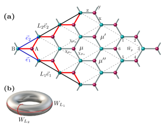
Figure 1: (a) The honeycomb lattice with $L_{1}=L_{2}=3$ and $M=0$ according to the explanations in the main text, where $\mu\ (\mu^{\prime},\mu^{\prime\prime})$ labels the unit cells (dashed parallelogram). The red links in direction $L_{i}\bm{e}_{i}$ denote the successive terms $\hat{\sigma}_{i}^{\alpha_{\langle ij\rangle}}\hat{\sigma}_{j}^{\alpha_{\langle ij\rangle}}$ in the topological loop operator $\hat{W}_{L_{i}}$ which also is sketched in (b) for clear observation.

II two-dimensional nonlinear spectroscopy

The definition and mathematical expression of the non-linear magnetic susceptibility is given in this section. The sample is imposed to two linearly polarized magnetic impulses in directions $\hat{e}_{\alpha}$ and $\hat{e}_{\beta}$ with $\tau_{1}$ time delay, i.e. $\bm{B}(t)=B_{\alpha}\delta(t)\hat{e}_{\alpha}+B_{\beta}\delta(t-\tau_{1})\hat{e}_{\beta}$. After the second pulse we wait a time interval $\tau_{2}$ when the magnetization in $\gamma$ direction is measured, $M_{\alpha\beta}^{\gamma}(\tau_{1}+\tau_{2})$. In order to eliminate the linear contributions in the response, two separate experiments are performed with a single pulse $B_{\alpha}$ or $B_{\beta}$ to measure the magnetizations $M_{\alpha}^{\gamma}(\tau_{1}+\tau_{2})$ or $M_{\beta}^{\gamma}(\tau_{1}+\tau_{2})$. Finally, the nonlinear response, $M^{\gamma}_{NL}$, is extracted by removing the linear magnetizations:

$$M^{\gamma}_{NL}(\tau_{1}+\tau_{2})=M_{\alpha\beta}^{\gamma}(\tau_{1}+\tau_{2})-M_{\alpha}^{\gamma}(\tau_{1}+\tau_{2})-M_{\beta}^{\gamma}(\tau_{1}+\tau_{2}).$$ (1)

We assume that the system is prepared in its ground state and the magnetization of ground state is zero, which is the case for QSLs. The weak magnetic field is coupled to the magnetization, $\hat{H}_{p}=-\bm{B}(t)\cdot\hat{M}$, which is considered in the framework of perturbation theoryChoi et al. (2020). Hence, the nonlinear magnetization is obtained as follows:

$$M^{\gamma}_{NL}(\tau_{1}+\tau_{2})/2N =B_{\alpha}B_{\beta}\chi^{(2),\gamma}_{\beta\alpha}(\tau_{2},\tau_{1})$$

$$+B_{\beta}B_{\alpha}B_{\alpha}\chi^{(3),\gamma}_{\beta\alpha\alpha}(\tau_{2},\tau_{1},0)$$

$$+B_{\beta}B_{\beta}B_{\alpha}\chi^{(3),\gamma}_{\beta\beta\alpha}(\tau_{2},0,\tau_{1})+\mathcal{O}(B^{4}),$$ (2)

where N is number of unit cells. The $n$-th order susceptibility is obtained from the $(n+1)$-points correlation functions,

$$\chi^{(2),\gamma}_{\beta\alpha}(\tau_{2},\tau_{1})=\frac{-1}{N}\sum_{l=1}^{2}\mathop{\mathrm{Re}}\nolimits\bigg{[}Q^{(l),\gamma}_{\beta\alpha}(\tau_{2},\tau_{1})\bigg{]},$$ (3)

where

$$Q^{(1),\gamma}_{\beta\alpha}(\tau_{2},\tau_{1}) =\langle\hat{M}_{I}^{\gamma}(\tau_{1}+\tau_{2})\hat{M}_{I}^{\beta}(\tau_{1})\hat{M}_{I}^{\alpha}(0)\rangle,$$

$$Q^{(2),\gamma}_{\beta\alpha}(\tau_{2},\tau_{1}) =-\langle\hat{M}_{I}^{\beta}(\tau_{1})\hat{M}_{I}^{\gamma}(\tau_{1}+\tau_{2})\hat{M}_{I}^{\alpha}(0)\rangle,$$ (4)

and

$$\chi^{(3),\gamma}_{\beta\alpha\alpha}(\tau_{2},\tau_{1},0) =\frac{1}{N}\sum_{l=1}^{4}\mathop{\mathrm{Im}}\nolimits\bigg{[}R^{(l),\gamma}_{\beta\alpha\alpha}(\tau_{2},\tau_{1},0)\bigg{]},$$ (5)

$$\chi^{(3),\gamma}_{\beta\beta\alpha}(\tau_{2},0,\tau_{1}) =\frac{1}{N}\sum_{l=1}^{4}\mathop{\mathrm{Im}}\nolimits\bigg{[}R^{(l),\gamma}_{\beta\beta\alpha}(\tau_{2},0,\tau_{1})\bigg{]},$$ (6)

in which

$$R^{(1),\gamma}_{\beta\eta\alpha}(t_{3},t_{2},t_{1}) =\langle\hat{M}_{I}^{\eta}(t_{1})\hat{M}_{I}^{\beta}(t_{1}+t_{2})\hat{M}_{I}^{\gamma}(t_{1}+t_{2}+t_{3})\hat{M}_{I}^{\alpha}(0)\rangle,$$

$$R^{(2),\gamma}_{\beta\eta\alpha}(t_{3},t_{2},t_{1}) =\langle\hat{M}_{I}^{\alpha}(0)\hat{M}_{I}^{\beta}(t_{1}+t_{2})\hat{M}_{I}^{\gamma}(t_{1}+t_{2}+t_{3})\hat{M}_{I}^{\eta}(t_{1})\rangle,$$

$$R^{(3),\gamma}_{\beta\eta\alpha}(t_{3},t_{2},t_{1}) =\langle\hat{M}_{I}^{\alpha}(0)\hat{M}_{I}^{\eta}(t_{1})\hat{M}_{I}^{\gamma}(t_{1}+t_{2}+t_{3})\hat{M}_{I}^{\beta}(t_{1}+t_{2})\rangle,$$

$$R^{(4),\gamma}_{\beta\eta\alpha}(t_{3},t_{2},t_{1}) =\langle\hat{M}_{I}^{\gamma}(t_{1}+t_{2}+t_{3})\hat{M}_{I}^{\beta}(t_{1}+t_{2})\hat{M}_{I}^{\eta}(t_{1})\hat{M}_{I}^{\alpha}(0)\rangle,$$ (7)

where $\eta=\alpha$ or $\beta$ and the subscript $I$ means the magnetization is calculated in the interaction picture. As we expect from the sequence of the magnetic impulses and the recorded signal after them, in the interaction picture the magnetizations $\hat{M}_{I}^{(\alpha)}$, $\hat{M}_{I}^{(\beta)}$ and $\hat{M}_{I}^{(\gamma)}$ always appear at times $(0),\ (t_{1}+t_{2})$, and $(t_{1}+t_{2}+t_{3})$, respectively.

III The model

The extended Kitaev model describes spin-1/2 degrees of freedom on the honeycomb lattice that is composed of the pure Kitaev terms along with three spin interactions. This model is an effective theory – which is obtained by a perturbative expansion Kitaev (2006)– to explain the effect of a weak magnetic field on Kitaev model,

$$H_{EK}=-\sum_{\langle ij\rangle_{\alpha}}J_{\alpha}\hat{\sigma}^{\alpha}_{i}\hat{\sigma}^{\alpha}_{j}-K\sum_{\begin{subarray}{c}\langle ik\rangle_{\alpha},\langle kj\rangle_{\beta}\\ \gamma\perp\alpha,\beta\end{subarray}}\hat{\sigma}^{\alpha}_{i}\hat{\sigma}^{\gamma}_{k}\hat{\sigma}^{\beta}_{j}.$$ (8)

In the last term the two bonds $\langle ik\rangle_{\alpha}$ and $\langle kj\rangle_{\beta}$ share the common site k. Following Refs. [Pedrocchi et al., 2011], we will consider the same labelling of spins and boundary conditions for the lattice, that is a honeycomb lattice with periodic boundary conditions in the direction of two base vectors $L_{1}\bm{e}_{1}$ and $L_{2}\bm{e}_{2}+M\bm{e}_{1}$, see Fig. 1-(a). In this geometry, the number of unit cells is $N=L_{1}L_{2}$.

For each plaquette $p$, Fig. 1-(a), the product of spins sitting on the corners is a constant of motion: $\hat{W}_{p}=\hat{\sigma}^{x}_{1}\hat{\sigma}^{y}_{2}\hat{\sigma}^{z}_{3}\hat{\sigma}^{x}_{4}\hat{\sigma}^{y}_{5}\hat{\sigma}^{z}_{6}$, which commutes with Hamiltonian and with other plaquette operators $[\hat{W_{p}},\hat{W_{p^{\prime}}}]=0$. Using the Kitaev parton construction, each spin is constructed with four Majorana fermions, the three static $\hat{b}_{i}^{x},\hat{b}_{i}^{y},$ and $\hat{b}_{i}^{z}$ and the dynamic $\hat{c}_{i}$ as followsKitaev (2006):

$$\hat{\sigma}_{i}^{\alpha}=i\hat{b}_{i}^{\alpha}\hat{c}_{i},\quad\alpha=x,y,z.$$ (9)

Using this representation we can rewrite the Hamiltonian ($H_{EK}$) in terms of Majorana fermions,

$$H_{EK}(\{u_{ij}\})=\frac{i}{2}\sum_{\langle ij\rangle_{\alpha}}J_{\alpha}\hat{u}_{\langle ij\rangle_{\alpha}}\hat{c}_{i}\hat{c}_{j} - \frac{i}{2}K\sum_{\begin{subarray}{c}\langle ik\rangle_{\alpha},\langle jk\rangle_{\beta}\\ \gamma\perp\alpha,\beta\end{subarray}}\epsilon_{\alpha\gamma\beta}\hat{u}_{\langle ik\rangle_{\alpha}}\hat{u}_{\langle jk\rangle_{\beta}}\hat{c}_{i}\hat{c}_{j},$$

$$\hat{u}_{\langle ij\rangle_{\alpha}} = i\hat{b}^{\alpha}_{i}\hat{b}^{\alpha}_{j},$$ (10)

where $\epsilon_{\alpha\gamma\beta}$ is the Levi-Civita symbol. Since $[\hat{H}_{EK},\hat{u}_{\langle ij\rangle_{\alpha}}]=0$ and $[\hat{u}_{\langle ij\rangle_{\alpha}},\hat{u}_{\langle ij\rangle_{\beta}}]=0$, for a given set of the bond variables $\{{u}_{\langle ij\rangle_{\alpha}}=\pm 1\}$, the Hamiltonian is reduced to a hopping problem of Majorana fermions, which can be solved exactly. $u_{ij}$ is an emergent $\mathbb{Z}_{2}$ gauge field, which makes the Hilbert space to be factorized into gauge $|\mathcal{G}\rangle$ and matter $|\mathcal{M}\rangle$ sectors. The physics of the spin Hamiltonian $H_{EK}$ is determined by the flux configurations $\{W_{p}=\prod_{\langle ij\rangle\in\partial p}u_{ij}\}$, where different gauge (bond) configurations $\{u_{ij}\}$ could give the same flux configuration. At a fixed flux sector the Hamiltonian takes the following compact form:Knolle et al. (2015)

$$H_{EK}=\frac{i}{2}\begin{pmatrix}\hat{c}_{A}^{T}&\hat{c}_{B}^{T}\end{pmatrix}\begin{pmatrix}F&M\\ -M^{T}&-G\end{pmatrix}\begin{pmatrix}\hat{c}_{A}\\ \hat{c}_{B}\end{pmatrix},$$ (11)

where $\hat{c}_{A(B)}$ is the column vector of all matter Majorana fermions on A (B) sublattice. $M$ is the first neighbor hopping matrix, while $F$ and $G$ are the second neighbor hopping matrices. In order to diagonalize $H_{EK}(\{u_{ij}\})$ in each flux sector, we introduce complex gauge and matter fermions that act on matter and gauge sectors, respectively Baskaran et al. (2007):

$$\hat{f}_{\mu_{z}}=\frac{1}{2}(\hat{c}_{\mu A}+i\hat{c}_{\mu B}),\quad\hat{\chi}_{\mu_{z}}=\frac{1}{2}(\hat{b}^{z}_{\mu A}-i\hat{b}^{z}_{\mu B}),$$

$$\hat{\chi}_{\mu_{y}}=\frac{1}{2}(\hat{b}^{y}_{\mu A}-i\hat{b}^{y}_{\mu^{\prime}B}),\quad\hat{\chi}_{\mu_{x}}=\frac{1}{2}(\hat{b}^{x}_{\mu A}-i\hat{b}^{x}_{\mu^{\prime\prime}B}).$$ (12)

According to our notation, $\mu$ labels the unit cells and $\mu_{a},a=x,y,z$ indicates the $x/y/z$-bond in that unit cell, which are shown in Fig. 1-(a). The gauge configuration $\{u_{ij}\}$, is determined by the occupation number of gauge fermions using the relation: $\hat{u}_{\langle ij\rangle_{\alpha}}=1-2\hat{\chi}^{\dagger}_{\langle ij\rangle_{\alpha}}\hat{\chi}_{\langle ij\rangle_{\alpha}}$. Hence, the Hamiltonian in each flux sector in terms of complex fermions ($\hat{f}$) takes this form:Knolle et al. (2015)

$$H_{EK}=\frac{1}{2}\begin{pmatrix}\hat{f}^{\dagger}&\hat{f}\end{pmatrix}\begin{pmatrix}h&\Delta\\ \Delta^{\dagger}&-h^{*}\end{pmatrix}\begin{pmatrix}\hat{f}\\ \hat{f}^{\dagger}\end{pmatrix},$$ (13)

where

$$h =(M^{T}+M)+i(F-G),\quad h^{\dagger}=h$$

$$\Delta =(M^{T}-M)+i(F+G),\quad\Delta^{T}=-\Delta.$$ (14)

Using the Bogoliubov transformation, $U$, as has been described in Refs. [Knolle et al., 2015,Blaizot and Ripka, 1985], the final Hamiltonian is diagonalized as follows

$$H_{EK}=\sum_{n}\varepsilon_{n}\hat{a}^{\dagger}_{n}\hat{a}_{n}-\frac{1}{2}\sum_{n}\varepsilon_{n},$$ (15)

where

$$\begin{pmatrix}\hat{a}\\ \hat{a}^{\dagger}\end{pmatrix}=U\begin{pmatrix}\hat{f}\\ \hat{f}^{\dagger}\end{pmatrix}.$$ (16)

Here, $\varepsilon_{n}\geq 0$ is the matter excitation energy and $\hat{a}^{\dagger}_{n}$($\hat{a}_{n}$) is the canonical fermionic creation (annihilation) operator. The last term in Eq.(15),

$$E=-\frac{1}{2}\sum_{n}\varepsilon_{n},$$ (17)

is the ground state energy (i.e., without matter excitations) in each flux sector.

III.1 Projection operator and the physical states

Representation of a spin with four Majorana operators has doubled the dimension of Hilbert space on each site of latticeMoessner and Moore (2021). Therefore, not all states in the extended Hilbert space $(\mathcal{H}_{EK})$ belong to the original physical spin Hilbert space. The states in the extended Hilbert space can be classified into physical and unphysical states by introducing the projection operator $\hat{\mathcal{P}}$ Kitaev (2006),

$$\hat{\mathcal{P}}=\prod_{i=1}^{2N}\bigg{(}\frac{1+\hat{D}_{i}}{2}\bigg{)},\quad\text{with:}\quad\hat{D}_{i}=\hat{b}_{i}^{x}\hat{b}_{i}^{y}\hat{b}_{i}^{z}\hat{c}_{i},$$

$$|\Psi_{\text{phys}}\rangle=\hat{\mathcal{P}}|\Psi_{u}\rangle.$$ (18)

Within a straightforward calculation we find that the projection operator can be written in the following formYao et al. (2009); Yao and Qi (2010)

$$\hat{\mathcal{P}}=\hat{\mathcal{S}}\hat{\mathcal{P}}_{0},$$

$$\hat{\mathcal{P}}_{0}=\frac{1+\hat{D}}{2},$$ (19)

where $\hat{D}=\prod_{i=1}^{2N}\hat{D}_{i}$ and $\hat{\mathcal{S}}$ sums symmetrically over all gauge-equivalent $\{u_{ij}\}$ configurations. For physical (unphysical) states we have $D=+1(-1)$. It has been shown that the operator $\hat{D}$ depends on the following values and parities Pedrocchi et al. (2011):

$$\hat{D}=(-1)^{\theta}\det(Q_{u})\hat{\pi}_{\chi}\hat{\pi}_{a}$$ (20)

where $\theta=L_{1}+L_{2}+M(L_{1}-M)$ and $Q_{u}$ is obtained by diagonalizing the Hamiltonian, see Appendix A. Moreover, $\hat{\pi}_{\chi}$ and $\hat{\pi}_{a}$ are the number parity of bond and matter fermions.

III.2 Physical ground state

The Wilson loop operator $\hat{W}_{\Gamma}$ associated with any closed loop $\Gamma$ on the lattice is a constant of motion for the Hamiltonian (8)Kitaev (2006); Halász et al. (2014):

$$\hat{W}_{\Gamma}=\hat{\sigma}_{i}^{\alpha_{\langle ij\rangle}}\hat{\sigma}_{j}^{\alpha_{\langle ij\rangle}}\hat{\sigma}_{j}^{\alpha_{\langle jk\rangle}}\hat{\sigma}_{k}^{\alpha_{\langle jk\rangle}}\dots\hat{\sigma}_{l}^{\alpha_{\langle li\rangle}}\hat{\sigma}_{i}^{\alpha_{\langle li\rangle}},$$ (21)

where $\{i,j,k,\dots,l\}$ refer to the sites on the loop and $\alpha_{\langle ij\rangle}=x,y,z$ shows the type of connecting link $\langle ij\rangle_{\alpha}$, i.e., the Wilson loop is the product of $x/y/z-$ Ising interactions on $x/y/z-$ links of the loop. The flux (plaquette) operator $\hat{W}_{p}$ is an elementary closed-loop operator such that any contractible closed-loop operator $\hat{W}_{\Gamma}$ on a torus can be constructed by multiplying a sequence of $\hat{W}_{p}$. On a torus (2D lattice with periodic boundary conditions), there are two non-contractible (topological) closed-loop operators that can not be construed by the product of plaquette operators. For example, in a system with the boundary condition $M=0$, these loop operators are $\hat{W}_{L_{1}}$ and $\hat{W}_{L_{2}}$ as shown with the red links in Fig.1-(a,b). The eigenvalues of these operators are $l_{1}=\pm 1$ and $l_{2}=\pm 1$. So, for any flux configuration $\{W_{p}\}$, there are four topologically inequivalent states, namely $|\{W_{p}\},l_{1},l_{2}\rangle$.

According to the Lieb’s theoremLieb (1994), we look for the physical ground state $(D=+1)$, in the 0-flux sector $\{W_{p}=+1,\forall p\}$. For simplicity, we consider a system with $L_{1}=L_{2}$ being an even number and $M=0$. Four topologically inequivalent states for the 0-flux sector can be constructed with the following gauge configurations:

$$|\{W_{p}=+1\},+1,+1\rangle=\hat{\mathcal{S}}|\mathcal{G}\rangle|\mathcal{M^{\prime++}}\rangle,$$

$$|\{W_{p}=+1\},+1,-1\rangle=\hat{\mathcal{S}}g_{+-}(\hat{\chi}^{\dagger})|\mathcal{G}\rangle|\mathcal{M^{\prime}}^{+-}\rangle,$$

$$|\{W_{p}=+1\},-1,+1\rangle=\hat{\mathcal{S}}g_{-+}(\hat{\chi}^{\dagger})|\mathcal{G}\rangle|\mathcal{M^{\prime}}^{-+}\rangle,$$

$$|\{W_{p}=+1\},-1,-1\rangle=\hat{\mathcal{S}}g_{--}(\hat{\chi}^{\dagger})|\mathcal{G}\rangle|\mathcal{M^{\prime}}^{--}\rangle,$$ (22)

where $|\mathcal{G}\rangle$ is the vacuum for the complex gauge fermions defined by the standard gauge configuration $\{u_{ij}=+1\}$ and $|\mathcal{M^{++}}\rangle$ is the vacuum for matter fermions in this gauge configuration. The operator $g_{l_{1}l_{2}}(\hat{\chi}^{\dagger})$ is the product of creation operators for complex gauge fermions which construct the gauge configuration with a specific topological label $(l_{1},l_{2})$ and $|\mathcal{M}^{l_{1}l_{2}}\rangle$ is the vacuum for matter fermions in the aforementioned gauge configuration $g_{l_{l}l_{2}}(\hat{\chi}^{\dagger})|\mathcal{G}\rangle$. The prime on the matter state $|\mathcal{M^{\prime}}^{l_{1}l_{2}}\rangle$ indicates that this state may have matter excitations, which is depends on the factor $(-1)^{\theta}\det(Q_{u})\hat{\pi}_{\chi}$ defined in Eq.(20). We have plotted the value of $(-1)^{\theta}\det(Q_{u})\hat{\pi}_{\chi}$ versus $K$ in Fig. 2 for the gauge configurations defined in Eq.(III.2) at the isotropic point $J_{x}=J_{y}=J_{z}=1$. According to Eq.(20) and Fig. 2, to reach a physical state with $D=+1$ the state with topological label $(+1,+1)$ must have an odd parity for matter excitations, while the other topological ground states have zero matter excitation. Based on our numerical evidences, we expect that for all even and odd values of the geometric parameters $L_{1}$, $L_{2}$, and $M$, the odd parity constraint for physical states with label $(+1,+1)$ in the 0-flux sector holds in the entire area of non-abelian phase of the extended Kitaev model, similar to the pure Kitaev modelZschocke and Vojta (2015). Accordingly, the states in Eq.(III.2) with minimum energy must have the following matter configurations,

$$|\mathcal{M^{\prime++}}\rangle=\hat{a}^{\dagger}_{1}|\mathcal{M^{++}}\rangle$$

$$|\mathcal{M^{\prime+-}}\rangle=|\mathcal{M^{+-}}\rangle,$$

$$|\mathcal{M^{\prime-+}}\rangle=|\mathcal{M^{-+}}\rangle,$$

$$|\mathcal{M^{\prime--}}\rangle=|\mathcal{M^{--}}\rangle.$$ (23)

It means the energy of $|\{W_{p}=+1\},+1,+1\rangle$ is $E^{(0)}+\varepsilon_{1}^{(0)}$, while the energy of the other three states is $E^{(0)}$, which is given by Eq.(17) within the 0-flux sectors and $\varepsilon_{1}^{(0)}$ is the first matter excitation in the same flux sector. Given $\varepsilon_{1}^{(0)}>0$ for any finite and non-zero value of $K$, the energy of the 0-flux state with the label $(+1,+1)$ is higher by the fermionic gap than the other three states in the groundstate manifold. Therefore, the topological groundstate in the non-Abelian phase of the extended model is three-fold degenerate as defined in Eq.(III.2) in agreement with the results presented in Ref. [Kells et al., 2009] using the Jordan-Wigner type transformation. It has to be mentioned that in Ref. [Kells et al., 2009] the transformation is in the original Hilbert space of the model and there is no unphysical degrees of freedom. Moreover, the non-Abelian phase supports three types of quasiparticles, namely: vacuum, Ising anyons, and fermions. Hence, in the framework of topological quantum field theory the groundstate on a torus has three-fold degeneracyNayak et al. (2008). In the Abelian phase of the model, we observed that for even value of $L_{1}$ and $L_{2}$ with $M=0$, the factor $(-1)^{\theta}\det(Q_{u})\hat{\pi}_{\chi}$ is always equal to $+1$ for all topologically inequivalent states, i.e, in this case, $|\mathcal{M^{\prime++}}\rangle=|\mathcal{M^{++}}\rangle$ and the groundstate subspace is composed of four degenerate states.

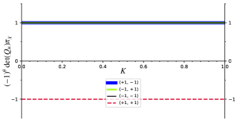
Figure 2: The value of $(-1)^{\theta}\det(Q_{u})\hat{\pi}_{\chi}$ versus $K$ for the four topological distinct states introduced in Eq.(III.2) labelled by ($l_{1},l_{2}$). The exchange couplings are in the non-Abelian phase with $J_{x}=J_{y}=J_{z}=1$ for a periodic system of $L_{1}=L_{2}=56,M=0$.

In order to calculate the nonlinear response of the system in the Abelian and non-Abelian phases, we can choose any state from the ground state manifold, because for 2DCS as a local probe, topologically inequivalent ground states are indistinguishable.

IV The nonlinear response

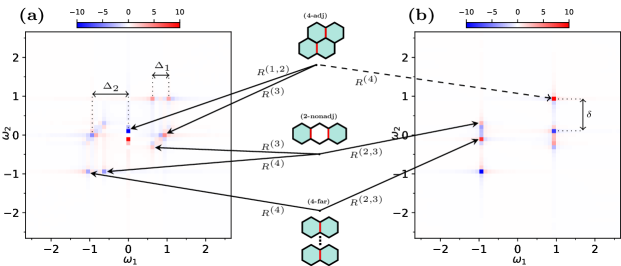
Figure 3: Two-dimensional nonlinear response in frequency domain at the isotropic point ($J_{x}=J_{y}=J_{z}=1$) in the non-Abelian phase with $K=0.2$. (a) $\chi^{(3),z}_{zzz}(\omega_{2},\omega_{1},0)$. (b) $\chi^{(3),z}_{zzz}(\omega_{2},0,\omega_{1})$. The dashed arrow indicates that the main contribution to the signal magnitude comes from the corresponding flux states. The solid arrows indicate that the signal comes only from the corresponding states. The black dots in the (4-far) class in the middle panel means that the flux separation is equal or more than two plaquettes. The maximum signal peak is normalized to 10.

The two-dimensional nonlinear susceptibilities introduced in Eq.(II) is calculated for the extended Kitaev model at polarization $(\alpha,\beta,\gamma)=(z,z,z)$. For the mentioned polarization, the second-order susceptibility is exactly zero, because by insertion of the resolution identity in the correlation functions $Q^{(l),\gamma}_{\beta\alpha}$, the overlap of flux sectors of the intermediate states vanishes Choi et al. (2020). We have used the few matter fermion approach, specifically the single matter fermion approximation Knolle et al. (2014a); which shows that the dynamical structure factor for small $K\text{'s}$ within this approximation gives almost the same results as the exact Paffian approach. To elaborate on this, it suffices to insert the resolution of identity into $R^{(1),\gamma}_{\beta\eta\alpha}$ correlation functions. For example, consider $R^{(1),z}_{zzz}(\tau_{2},\tau_{1},0)=R^{(2),z}_{zzz}(\tau_{2},\tau_{1},0)\doteq R^{(1,2),z}_{zzz}(\tau_{2},\tau_{1},0)$:

$$R^{(1,2),z}_{zzz}(\tau_{2},\tau_{1},0)=\langle\hat{M}_{I}^{z}(0)\mathds{1}\hat{M}_{I}^{z}(\tau_{1})\mathds{1}\hat{M}_{I}^{z}(\tau_{1}+\tau_{2})\mathds{1}\hat{M}_{I}^{z}(0)\rangle$$

$$=\sum_{\mu\nu\lambda\rho}\sum_{PQR}\langle G|\hat{Z}_{\mu}|P\rangle\langle P|\hat{Z}_{\nu}|Q\rangle\langle Q|\hat{Z}_{\lambda}|R\rangle\langle R|\hat{Z}_{\rho}|G\rangle$$

$$\quad\quad\quad\quad\times e^{i[E_{P}\tau_{1}+E_{Q}\tau_{2}-E_{R}(\tau_{1}+\tau_{2})]},$$ (24)

where $\hat{Z}_{\mu}=\hat{\sigma}^{z}_{\mu A}+\hat{\sigma}^{z}_{\mu B}$, is the sum of the Pauli z-matrix of the two spins on the $\mu$-th cell. Moreover, $|G\rangle$ is the ground state, $|P\rangle$, $|Q\rangle$ and $|R\rangle$ represent an eigenstate of the Hamiltonian. The matrix elements appeared in Eq.(IV) are the same for other $R^{(1),z}_{zzz}$ functions, which differ only in the phase factor. The eigenstates with different flux sectors are orthogonal to each other, hence the matrix elements in Eq.(IV) are non-zero only for the four $\hat{Z}_{\mu}$ operators with the following sequence of indices: $\hat{Z}_{m}\hat{Z}_{n}\hat{Z}_{n}\hat{Z}_{m}$, $\hat{Z}_{m}\hat{Z}_{n}\hat{Z}_{m}\hat{Z}_{n}$, and, $\hat{Z}_{m}\hat{Z}_{m}\hat{Z}_{n}\hat{Z}_{n}$. The last case, in the single matter approximation produces a term, which grows linearly with the system size. However, according to Eq.(II), the nonlinear susceptibilities are independent of the system size, hence, we exclude this contributionChoi et al. (2020). The two former cases result in the following matrix elements,

$$\sum_{\mu\nu}\langle G|\hat{Z}_{\mu}|P_{\mu}\rangle\langle P_{\mu}|\hat{Z}_{\nu}|Q_{\mu\nu}\rangle\langle Q_{\mu\nu}|\hat{Z}_{\nu}|R_{\mu}\rangle\langle R_{\mu}|\hat{Z}_{\mu}|G\rangle,$$

$$\sum_{\mu\nu}\langle G|\hat{Z}_{\nu}|P_{\nu}\rangle\langle P_{\nu}|\hat{Z}_{\mu}|Q_{\mu\nu}\rangle\langle Q_{\mu\nu}|\hat{Z}_{\nu}|R_{\mu}\rangle\langle R_{\mu}|\hat{Z}_{\mu}|G\rangle.$$ (25)

According to the single matter approximation we choose the states in Eq.(IV) as follows:

$$\begin{cases}|G\rangle=\hat{\mathcal{S}}g_{+-}(\hat{\chi}^{\dagger})|\mathcal{G}\rangle|\mathcal{M}^{+-}\rangle\\ |{R_{\mu}}\rangle=\hat{\mathcal{S}}\hat{\chi}_{\mu_{z}}^{\dagger}g_{+-}(\hat{\chi}^{\dagger})\overline{\hat{a}}_{r}^{\dagger}|{\mathcal{G}}\rangle|\mathcal{M}_{\mu}^{+-}\rangle\hskip 22.76219pt(\mbox{2-flux state})\\ |{Q_{\mu\nu}}\rangle=\hat{\mathcal{S}}\hat{\chi}_{\mu_{z}}^{\dagger}\hat{\chi}_{\nu_{z}}^{\dagger}g_{+-}(\hat{\chi}^{\dagger})|{\mathcal{G}}\rangle|\mathcal{M}_{\mu\nu}^{+-}\rangle\hskip 14.22636pt\ (\mbox{2 or 4-flux state}),\end{cases}$$ (26)

where $\overline{\hat{a}}_{r}^{\dagger}$ denotes a fermion creation operator in the 2-flux state $|R_{\mu}\rangle$ and $|\mathcal{M_{\mu}^{+-}}\rangle$, $|\mathcal{M_{\mu\nu}^{+-}}\rangle$ are the vacuum for matter fermions. In our calculations, we consider the state with topological label $(+1,-1)$ for the ground state of nonlinear response in the Abelian and non-Abelian phases.

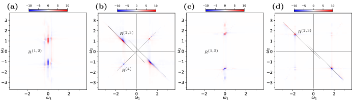
Figure 4: Two-dimensional nonlinear susceptibilities in frequency domain at an anisotropic point in the Abelian phase with $K=0.2$. (a) $\chi^{(3),z}_{zzz}(\omega_{2},\omega_{1},0)$ and (b) $\chi^{(3),z}_{zzz}(\omega_{2},0,\omega_{1})$ with $J_{x}=1,J_{y}=J_{z}=0.3$. (c) $\chi^{(3),z}_{zzz}(\omega_{2},\omega_{1},0)$ and (d) $\chi^{(3),z}_{zzz}(\omega_{2},0,\omega_{1})$ with $J_{x}=1,J_{y}=J_{z}=0.05$. In (b) and (d) the shifted diagonal signals intercept $\omega_{1}$ and $\omega_{2}$ axes at $|E_{4}-E_{0}|=0.276$ and $0.125$, respectively. The magnitude of the maximum peak of susceptibility in all plots is normalized to 10.

IV.1 Results

The Fourier transform of two-dimensional nonlinear magnetic susceptibilities, $\chi^{(3),z}_{zzz}(\omega_{2},\omega_{1},0)$ and $\chi^{(3),z}_{zzz}(\omega_{2},0,\omega_{1})$, are shown in Fig. 3 for a system with ($33\times 33$) unit cells, $J_{x}=J_{y}=J_{z}=J=1$ and $K=0.2$. We use the fast Fourier transformation to obtain the Fourier spectrum from time domaincom . In the non-Abelian phase of the model, the energy of a flux state depends on the distance between its vorticesLahtinen et al. (2008); Lahtinen (2011), accordingly the states $|Q_{1\mu}\rangle$ in the nonlinear response can be classified into three classes: 4-adjacent, 2-non-adjacent, 4-far-separated, as depicted in the middle panel of Fig. 3. By considering the contribution of states in each of these classes individually, we can determine the origin of sharp peaks in the observed response. The origin of each peak in the response in terms of the mentioned classes are indicated by the corresponding arrows in the middle panel of Fig. 3. A black arrow pointing to a spot in response stipulates the origin of that signal comes only from the mentioned excitations, while the dashed arrow indicates an excitation which has the main contributions to the signal. The observation of peaks corresponding to flux sectors with 4-adjacent, 2-non-adjacent, and 4-far-separated fluxes is a new signature of flux excitations that does not appear in the linear responses. Due to the fact that the extended model has a gapped spectrum, a system with $(33\times 33)$ unit cells is large enough to reach the thermodynamic limit for $K=0.2$. The finite size effects is discussed in the appendix (See Fig.(7)), where we present the difference between physical responses in Fourier space for different system sizes. As the system size increases to $L=33$, the aforementioned difference becomes almost zero, which convinces us to reach enough large system sizes. The three energy scales $\Delta_{1}$, $\Delta_{2}$, and $\delta$ can be extracted from the nonlinear response, as depicted in Fig. 3,

$$\Delta_{1}=(E^{(4\text{far})}-E^{(0)})-(E^{(2\text{nonadj})}-E^{(0)})=E^{(4\text{far})}-E^{(2\text{nonadj})},$$

$$\Delta_{2}=E^{(4\text{adj})}-E^{(0)},$$

$$\delta=(\varepsilon_{1}^{(2)}+E^{(2)}-E^{(0)})-(E^{(4\text{far})}-E^{(2)}-\varepsilon_{1}^{(2)})\approx 2\varepsilon_{1}^{(2)},$$

where $E^{(4\text{adj})}$, $E^{(2\text{nonadj})}$, and $E^{(4\text{far})}$ are the ground state energy of the flux states depicted in the middle of Fig. 3. Moreover, $\varepsilon_{1}^{(2)}$ is the in-gap energy of two-adjacent flux state. For the considered parameters in Fig.  3 we obtain $(\Delta_{1},\Delta_{2},\delta)=(0.434,0.894,0.758)$. The signature of an in-gap bound state $\delta$ can be also detected in the linear response as a sharp peak in the dynamical spin structure factorKnolle et al. (2015), while $\Delta_{1}$ and $\Delta_{2}$ are new signature of flux states of the non-Abelian anyons, which appear only in the nonlinear responses.

We have also obtained the nonlinear response of the Abelian phase. The Fourier transform of the third-order susceptibilities for the Abelian phase are presented in Fig. 4. In all plots of Fig. 4 we keep $J_{x}=1$ and $K=0.2$, the couplings in parts (a) and (b) are $J=J_{y}=J_{z}=0.3$ and the system has $N=44\times 44$ unit cells, while in parts (c) and (d) we have $J=J_{y}=J_{z}=0.05$ and $N=28\times 28$ unit cells.

We observe weak diagonal signals (the first and third quadrants) and strong shifted diagonal signals (the second and fourth quadrants) in Fig. 4-(b) for $J=0.3$ in $\chi^{(3),z}_{zzz}(\omega_{2},0,\omega_{1})$. The diagonal signals come from the $R^{(4),z}_{zzz}(\omega_{2},0,\omega_{1})$ expression, in which there are two delta functions with peak frequencies:

$$\omega_{1}=E_{0}-E_{2}-\varepsilon_{r}^{(2)},\quad\quad\omega_{2}=E_{0}-E_{2}-\varepsilon_{p}^{(2)},$$ (28)

where $\varepsilon_{r/p}^{(2)}$ is the matter excitations in the 2-flux state $|R\rangle/|P\rangle$. Whenever $|R\rangle=|P\rangle$, there is a constructive interference for matrix elements,Choi et al. (2020) which leads to the diagonal signal (non-rephasing signal), $\omega_{1}=\omega_{2}$. Moreover, the expression $R^{(2,3),z}_{zzz}(\omega_{2},0,\omega_{1})$ is responsible for the shifted diagonal signals, which contains two peaks at:

$$\omega_{1}=E_{2}-E_{0}+\varepsilon_{p}^{(2)},\quad\quad\omega_{2}=E_{4}-E_{2}-\varepsilon_{r}^{(2)}.$$ (29)

This leads to the strong streak signal (rephasing signal) $\omega_{1}+\omega_{2}=E_{4}-E_{0}$ for $|R\rangle=|P\rangle$ due to constructive interference. This signal intercepts $\omega_{2}$-axis at $E_{4}-E_{0}$.

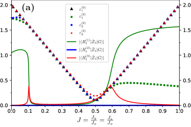
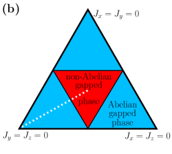
Figure 5: (color online) (a) The evolution path versus $J$ for the lowest eigenvalue in the 0-flux sector ($\varepsilon_{1}^{(0)}$), 2-adjacent flux sector ($\varepsilon_{r}^{(2)}$) and the matrix element $|\langle R_{\mu=1}^{(r)}|\hat{Z}_{\mu=1}|G\rangle|$ for the three lowest excitation modes $r=1,2,3$ in the two-flux state $|R_{1}^{(r)}\rangle$. By increasing the size of the system, the fermionic gap $\varepsilon_{1}^{(0)}$ is closed at the phase transition point $J=0.5$ in (a). These presented data come from a system with $L_{1}=L_{2}=56,\ M=0$. (b) The phase diagram of extended Kitaev model in the plane $J_{x}+J_{y}+J_{z}=\mbox{constant}$, where the dotted white line shows the evolution path of part (a).

However, in Fig. 4-(d), at $J=0.05$ the diagonal signal does not show up and the shifted diagonal signal is very weak, where only sharp spots appear in the responses. To investigate this difference, we examine the absolute value of $\langle R_{\mu}|\hat{Z}_{\mu}|G\rangle$ as a relevant matrix element to the nonlinear response versus $J$ within the single matter approximation, for the three excited states labelled by $r=1,2,3$. The excited states are expressed by $|R_{\mu}^{(r)}\rangle=\hat{\mathcal{S}}\hat{\chi}_{\mu_{z}}^{\dagger}g_{+-}(\hat{\chi}^{\dagger})\overline{\hat{a}}_{r}^{\dagger}|{\mathcal{G}}\rangle|\mathcal{M}^{\mu}_{+-}\rangle$ as given in Eq.(26). A simple expression for this matrix element is given in Appendix(B). Fig. 5-(a) shows the first matter eigenvalue $\varepsilon^{(0)}_{1}$ in the 0-flux state $|G\rangle$ as well as $|\langle R_{\mu}^{(r)}|\hat{Z}_{\mu}|G\rangle|$ for $r=1,2,3$ corresponding to the lowest excitation modes $\bar{\hat{a}}^{\dagger}_{1}$, $\bar{\hat{a}}^{\dagger}_{2}$, and $\bar{\hat{a}}^{\dagger}_{3}$ in the two-flux state $|R_{1}^{(r)}\rangle$ and their corresponding eigenvalues $\varepsilon^{(2)}_{1}$, $\varepsilon^{(2)}_{2}$ , and $\varepsilon^{(2)}_{3}$. The coupling $J$ in Fig. 5-(a) varies from $0$ to $1$, which is shown by the dotted white path in Fig.5-(b). We anticipate that in the Abelian phase for $K=0.2,$ the diagonal and shifted diagonal signals to appear in the range $0.1<J<0.5$, because low-energy excitation modes have almost equal contributions to the response, which leads to a continuum of spots. However, for $0<J<0.1$, the excitation mode $r=1$ has the dominant matrix element compared with the other excitation modes. Hence, the main contribution comes from $r=1$, and as a result, we only observe sharp spot in the response function. According to Fig. 5-(a), we anticipate that in the non-Abelian phase for $K=0.2$ and $J>0.6$, the pattern of nonlinear spectrum is formed by sharp spots, similar to what we see in Fig. 3 for the isotropic case. We have plotted the nonlinear response along the white path of Fig.5-(b) for several values of $J$ in Fig.8 of Appendix D, which justifies our statement. For details see Appendix D.

The presence and absence of streak signals in the nonlinear response of the Abelian phase of EKM can also be understood in terms of an effective theory where $J_{x}\gg J_{y},J_{z},K$. Deep in the Abelian phase (close to the corners of the triangle in Fig.5-(b)), the effective Hamiltonian of EKM is the Kitaev toric code, where the first nonzero term appears in the second order perturbation theory (see Appendix E). The toric code has sharp charge (e) and flux (m) excitations without any dispersion. Therefore, it is reasonable to observe sharp peaks in the nonlinear response of Fig.4-(c,d). However, by digressing from the toric code limit (away from the corners), the excitations become dispersed and the streak signals appear as discussed earlier and presented in Fig.4-(a, b).

V Discussions and Conclusions

We numerically studied the nonlinear response of extended Kitaev model in its Abelian and non-Abelian phases by using two-dimensional coherent spectroscopy. The numerical computations are restricted to finite systems with periodic boundary conditions with the lattice geometry, which has been introduced in Ref. [Pedrocchi et al., 2011] in order to explicitly determine the physical and unphysical states of the Kitaev solution. This is important, because physical quantities must be calculated in the physical subspace.

The nonlinear response of the pure Kitaev model at the isotropic pointChoi et al. (2020) has diagonal and shifted-diagonal streak signals in the 2D frequency space $\omega_{1}$-$\omega_{2}$, however in the extended Kitaev model, these streak signals are very weak and practically no longer exist, where only sharp spots are seen in the response. The sharp spots are only due to flux excitations and in-gap bound states. Away from the triangular phase boundary in the non-Abelian phase including the isotropic point of the extended Kitaev model we expect similar sharp spots in the nonlinear response. Distinct signatures of different flux excitations can be discerned within the nonlinear spectroscopic approach. These new features of flux excitations can not be observed in the linear response.

In the Abelian phase distinct signatures of fractionalized quasiparticles appear in the nonlinear response. For two sets of parameters $J_{y}=J_{z}=0.3$ and $J_{y}=J_{z}=0.05$ with $J_{x}=1$ and $K=0.2$, we obtain relatively different nonlinear responses. In the former case, there are strong streak signals which are signatures of dynamical Majorana fermions ($\hat{c}_{i}$) in addition to their $\omega_{1}$-/$\omega_{2}$-intercept as indications of nondynamical Majorana fermions ($\hat{b}_{i}^{x},\hat{b}_{i}^{y},\hat{b}_{i}^{z}$). While in the later case, where one of the Kitaev exchange couplings is much stronger than the others, the streak signals are very weak and only sharp spots show up. The mentioned sharp spots are signature of an effective behavior in terms of conventional toric code. It looks like a cross over between two different dynamical responses in the Abelian phase.

The general form of our presented results are similar to the nonlinear spectroscopic fingerprints of gapped spin liquids, which have been reported in Ref. [Nandkishore et al., 2021]. The difference stems from the fact that in the EKM there are two types of excitations, flux excitations (similar to e and m excitations in toric code model) and matter excitations that change energy scales and shift the sharp spots in the responses. If we ignore the matter excitations in our calculations, for instance discarding $\varepsilon_{r/p}^{(2)}$ in Eq.(29), we will obtain the same responses as in Ref. [Nandkishore et al., 2021]. It has to be stressed that the time-reversal symmetry is broken in EKM in contrast to the models considered in Ref. [Nandkishore et al., 2021].

The nonlinear responses presented in this work may be applicable to Kitaev quantum spin liquid candidates in weak magnetic fields. We did not take into account the effect of finite temperature, disorders, and interactions that could be relevant to explain experimental results, which are proposed for future works.

Appendix A The $Q_{u}$ matrix

In order to specify the physical and unphysical states by determining the sign of the $D$ in Eq.(20), we first construct the $Q_{u}$ matrix. This is achieved by using the Bogoliubov transformation $U$ that diagonalizes the Hamiltonian in Eq.(13) as follows

$$U\begin{pmatrix}h&\Delta\\ -\Delta^{*}&-h^{*}\end{pmatrix}U^{\dagger}=\begin{pmatrix}\bm{\varepsilon}&0\\ 0&-\bm{\varepsilon}\end{pmatrix},\quad U\begin{pmatrix}\hat{f}\\ \hat{f}^{\dagger}\end{pmatrix}=\begin{pmatrix}\hat{a}\\ \hat{a}^{\dagger}\end{pmatrix}\quad\Longrightarrow\hat{H}_{u}=\sum_{n}\varepsilon_{n}\hat{a}^{\dagger}_{n}\hat{a}_{n}-\frac{1}{2}\sum_{n}\varepsilon_{n},$$ (30)

where $\bm{\varepsilon}$ is a diagonal matrix with entries $\varepsilon_{n}\geq 0$. Because $\hat{a}$ and $\hat{a}^{\dagger}$ are hermitian conjugates of each other, the matrix $U$ can be generally written as

$$U=\begin{pmatrix}X^{*}&Y^{*}\\ Y&X\end{pmatrix}.$$ (31)

The matrix $U$ can be derived from eigenvectors of the Hamiltonian. Suppose that $V^{n}$ is an eigenvector of the Hamiltonian with eigenvalue $\varepsilon_{n}$,

$$V^{n}=\begin{pmatrix}x^{n}\\ y^{n}\end{pmatrix},$$ (32)

where $x^{n}$ and $y^{n}$ are $N$-dimensional column vectors. Due to the particle-hole symmetry: $\Xi\hat{H}_{u}\Xi^{-1}=-\hat{H}_{u}$, $W_{n}=\Xi V_{n}$ is also an eigenvector for the Hamiltonian with the eigenvalue $-\varepsilon_{n}$,

$$W^{n}=\Xi V^{n}=(\tau_{x}\mathcal{K})V^{n}=\begin{pmatrix}0&1\\ 1&0\end{pmatrix}{V^{n}}^{*}=\begin{pmatrix}{y^{n}}^{*}\\ {x^{n}}^{*}\end{pmatrix}.$$ (33)

Using the fact that the eigenvectors of $\hat{H}_{u}$ are the column vectors of $U^{-1}$, we have

$$U^{-1}=\begin{pmatrix}x^{1}&x^{2}&\dots&x^{N}&{y^{1}}^{*}&{y^{2}}^{*}&\dots&{y^{N}}^{*}\\ y^{1}&y^{2}&\dots&y^{N}&{x^{1}}^{*}&{x^{2}}^{*}&\dots&{x^{N}}^{*}\end{pmatrix}.$$ (34)

Since $U$ is a unitary matrix, the matrices $X$ and $Y$ in (31) are given as follows:

$$X=\begin{pmatrix}x^{1}&x^{2}&\dots&x^{N}\end{pmatrix}^{T},\quad Y=\begin{pmatrix}y^{1}&y^{2}&\dots&y^{N}\end{pmatrix}^{T}.$$ (35)

The physical and unphysical states are determined by specifying the sign of $\hat{D}$ operator: $\hat{D}=(-1)^{\theta}\det(Q_{u})\hat{\pi}_{\chi}\hat{\pi}_{a}$, where

$$\hat{\pi}_{\chi}=\hat{\pi}_{\chi_{x}}\hat{\pi}_{\chi_{y}}\hat{\pi}_{\chi_{z}},$$

$$\hat{\pi}_{\chi_{\alpha}}=\prod_{\mu=0}^{N-1}(1-2\hat{\chi}^{\dagger}_{\mu_{\alpha}}\hat{\chi}_{\mu_{\alpha}})=\prod_{\mu=0}^{N-1}i\hat{b}_{\mu A}^{\alpha}\hat{b}_{\mu B}^{\alpha}=\prod_{\mu}\hat{u}_{\mu_{\alpha}},$$

$$\hat{\pi}_{a}=\prod_{k=0}^{N-1}(1-2\hat{a}^{\dagger}_{k}\hat{a}_{k})=(-1)^{\sum_{k}\hat{a}^{\dagger}_{k}\hat{a}_{k}},$$ (36)

and $Q_{u}$ is an orthogonal transformation defined in Ref. [Pedrocchi et al., 2011] as given below,

$$(\hat{b}_{1}^{\prime},\hat{b}_{1}^{\prime\prime},\hat{b}_{2}^{\prime},\hat{b}_{2}^{\prime\prime},\dots,\hat{b}_{N}^{\prime},\hat{b}_{N}^{\prime\prime})=(\hat{c}_{1},\hat{c}_{2},\hat{c}_{3},\dots,\hat{c}_{N})Q_{u},$$ (37)

where $\hat{b}^{\prime}$ and $\hat{b}^{\prime\prime}$ are fermion operators that are related to the canonical fermion operators according to the following relations

$$\hat{a}_{k}=\frac{1}{2}(\hat{b}_{k}^{\prime}+i\hat{b}_{k}^{\prime\prime}),\quad\hat{a}_{k}^{\dagger}=\frac{1}{2}(\hat{b}_{k}^{\prime}-i\hat{b}_{k}^{\prime\prime})\quad\Longrightarrow\begin{pmatrix}\hat{a}\\ \hat{a}^{\dagger}\end{pmatrix}=\frac{1}{2}\begin{pmatrix}1&i\\ 1&-i\end{pmatrix}\begin{pmatrix}\hat{b}^{\prime}\\ \hat{b}^{\prime\prime}\end{pmatrix}.$$ (38)

To find the $Q_{u}$ matrix, we need to find the transformation between $\hat{b}^{\prime}$/$\hat{b}^{\prime\prime}$ and $\hat{c}_{A}$/$\hat{c}_{B}$ fermion operators. Firstly, we use Eq.(III) and Eq.(16),

$$\begin{pmatrix}\hat{a}\\ \hat{a}^{\dagger}\end{pmatrix}=U\begin{pmatrix}\hat{f}\\ \hat{f}^{\dagger}\end{pmatrix},\quad\begin{pmatrix}\hat{f}\\ \hat{f}^{\dagger}\end{pmatrix}=\frac{1}{2}\begin{pmatrix}1&i\\ 1&-i\end{pmatrix}\begin{pmatrix}\hat{c}_{A}\\ \hat{c}_{B}\end{pmatrix}\quad\Longrightarrow\begin{pmatrix}\hat{a}\\ \hat{a}^{\dagger}\end{pmatrix}=\frac{1}{2}U\begin{pmatrix}1&i\\ 1&-i\end{pmatrix}\begin{pmatrix}\hat{c}_{A}\\ \hat{c}_{B}\end{pmatrix}.$$ (39)

Then, we take into account Eq.(38) and Eq.(39), which lead to

$$\begin{pmatrix}\hat{b}^{\prime}\\ \hat{b}^{\prime\prime}\end{pmatrix}=Q_{u}^{\prime}\begin{pmatrix}\hat{c}_{A}\\ \hat{c}_{B}\end{pmatrix},\quad Q_{u}^{\prime}=\begin{pmatrix}\mathop{\mathrm{Re}}\nolimits[A]&\mathop{\mathrm{Im}}\nolimits[B]\\ -\mathop{\mathrm{Im}}\nolimits[A]&\mathop{\mathrm{Re}}\nolimits[B]\\ \end{pmatrix},$$ (40)

where $A=X+Y$ and $B=X-Y$. According to the labelling of fermion operators within each unit cell we have

$$\begin{pmatrix}\hat{c}_{A}\\ \hat{c}_{B}\end{pmatrix}=\begin{pmatrix}\hat{c}_{2}\\ \hat{c}_{4}\\ \vdots\\ \hat{c}_{2N}\\ \hat{c}_{1}\\ \hat{c}_{3}\\ \vdots\\ \hat{c}_{2N-1}\end{pmatrix}=R_{c}\begin{pmatrix}\hat{c}_{1}\\ \hat{c}_{2}\\ \hat{c}_{3}\\ \hat{c}_{4}\\ \vdots\\ \vdots\\ \vdots\\ \hat{c}_{2N}\end{pmatrix},\quad R_{c}=\begin{pmatrix}0&1&0&0&0&\dots&0&0&0\\ 0&0&0&1&0&\dots&0&0&0\\ &&&&&\vdots&&&\\ 0&0&0&0&0&\dots&0&0&1\\ 1&0&0&0&0&\dots&0&0&0\\ 0&0&1&0&0&\dots&0&0&0\\ &&&&&\vdots&&&\\ 0&0&0&0&0&\dots&0&1&0\end{pmatrix}_{2N\times 2N},$$ (41)

$$\begin{pmatrix}\hat{b}^{\prime}\\ \hat{b}^{\prime\prime}\end{pmatrix}=\begin{pmatrix}\hat{b}_{1}^{\prime}\\ \hat{b}_{2}^{\prime}\\ \vdots\\ \hat{b}_{N}^{\prime}\\ \hat{b}_{1}^{\prime\prime}\\ \hat{b}_{2}^{\prime\prime}\\ \vdots\\ \hat{b}_{N}^{\prime\prime}\\ \end{pmatrix}=R_{b}\begin{pmatrix}\hat{b}_{1}^{\prime}\\ \hat{b}_{1}^{\prime\prime}\\ \hat{b}_{2}^{\prime}\\ \hat{b}_{2}^{\prime\prime}\\ \vdots\\ \vdots\\ \hat{b}_{N}^{\prime}\\ \hat{b}_{N}^{\prime\prime}\end{pmatrix},\quad R_{b}=\begin{pmatrix}1&0&0&0&0&\dots&0&0&0\\ 0&0&1&0&0&\dots&0&0&0\\ &&&&&\vdots&&&\\ 0&0&0&0&0&\dots&0&1&0\\ 0&1&0&0&0&\dots&0&0&0\\ 0&0&0&1&0&\dots&0&0&0\\ &&&&&\vdots&&&\\ 0&0&0&0&0&\dots&0&0&1\end{pmatrix}_{2N\times 2N}.$$ (42)

Finally, using Eqs.(40), (41), and (42), we arrive at the desired relation,

$$(\hat{b}_{1}^{\prime},\hat{b}_{1}^{\prime\prime},\dots,\hat{b}_{N}^{\prime},\hat{b}_{N}^{\prime\prime})=(\hat{c}_{1},\hat{c}_{2},\hat{c}_{3},\dots,\hat{c}_{2N})\bigg{[}R_{b}^{-1}Q_{u}^{\prime}R_{c}\bigg{]}^{T}\quad\Longrightarrow Q_{u}=\bigg{[}R_{b}^{-1}Q_{u}^{\prime}R_{c}\bigg{]}^{T}.$$ (43)

With this important matrix we can find the parity $\hat{\pi}_{c}=\prod_{\mu=1}^{N}i\hat{c}_{\mu A}\hat{c}_{\mu B}$ in terms of the parity of canonical matter fermionsPedrocchi et al. (2011):

$$\hat{\pi}_{c}=\det(Q_{u})\hat{\pi}_{a}.$$ (44)

Appendix B Gauge configurations, Matrix elements, and $R^{(l),z}_{zzz}$ correlation functions

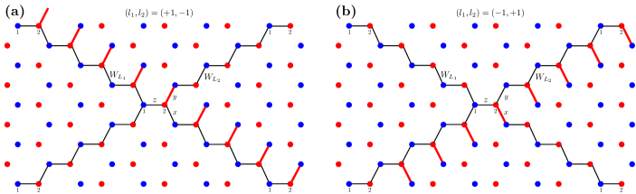
Figure 6: Gauge configuration for two degenerate ground states with different topological labels for a finite system with $L_{1}=L_{2}=4$ and $M=0$. (a) and (b) show the gauge configuration that we adopted for $g_{+-}(\hat{\chi}^{\dagger})|\mathcal{G}\rangle$ and $g_{-+}(\hat{\chi}^{\dagger})|\mathcal{G}\rangle$, respectively. The black strings links represent the topological loop operators $W_{L_{1}}$ and $W_{L_{2}}$, which are reduced to the product of $u_{ij}$’s on these links in a fixed gauge configuration. The red links show the position of links, where $u_{ij}=-1$.

According to subsection (III.2), the ground state $|G\rangle$ in the non-Abelian phase has a 3-fold degeneracy on a torus with topological labels $(+1,-1)$, $(-1,+1)$, and $(-1,-1)$. Fig. 6-(a) and Fig. 6-(b) show the gauge configurations $g_{+-}(\hat{\chi}^{\dagger})|\mathcal{G}\rangle$ and $g_{-+}(\hat{\chi}^{\dagger})|\mathcal{G}\rangle$ for a finite system; designed by red links $u_{\langle ij\rangle_{\alpha}}=-1$. The gauge configuration $g_{--}(\hat{\chi}^{\dagger})|\mathcal{G}\rangle$ is obtained by taking into account the gauge configurations presented in Figs. 6-(a, b), simultaneously, i.e., $g_{--}(\hat{\chi}^{\dagger})=g_{+-}(\hat{\chi}^{\dagger})g_{-+}(\hat{\chi}^{\dagger})$.

To calculate the matrix elements in the correlation functions $R^{(l),z}_{zzz}$, it is necessary to find the relation between the matter ground states of different flux sectors. Let $|\mathcal{M}_{F_{1}}\rangle$ and $|\mathcal{M}_{F_{2}}\rangle$ be the ground states of flux sectors $F_{1}$ and $F_{2}$, respectively. Creation and annihilation operators in each sector are given as follows,

$$\begin{pmatrix}\hat{a}_{F_{1}}\\ \hat{a}^{\dagger}_{F_{1}}\end{pmatrix}=\begin{pmatrix}X^{*}_{F_{1}}&Y^{*}_{F_{1}}\\ Y_{F_{1}}&X_{F_{1}}\end{pmatrix}\begin{pmatrix}\hat{f}\\ \hat{f}^{\dagger}\end{pmatrix}\quad,\quad\begin{pmatrix}\hat{a}_{F_{2}}\\ \hat{a}^{\dagger}_{F_{2}}\end{pmatrix}=\begin{pmatrix}X^{*}_{F_{2}}&Y^{*}_{F_{2}}\\ Y_{F_{2}}&X_{F_{2}}\end{pmatrix}\begin{pmatrix}\hat{f}\\ \hat{f}^{\dagger}\end{pmatrix},$$ (45)

which are related to each other by the following transformation:

$$\begin{pmatrix}\hat{a}_{F_{2}}\\ \hat{a}^{\dagger}_{F_{2}}\end{pmatrix}=\begin{pmatrix}\mathcal{X}^{*}_{F_{2},F_{1}}&\mathcal{Y}^{*}_{F_{2},F_{1}}\\ \mathcal{Y}_{F_{2},F_{1}}&\mathcal{X}_{F_{2},F_{1}}\end{pmatrix}\begin{pmatrix}\hat{a}_{F_{1}}\\ \hat{a}^{\dagger}_{F_{1}}\end{pmatrix}\quad,\quad\begin{pmatrix}\mathcal{X}^{*}_{F_{2},F_{1}}&\mathcal{Y}^{*}_{F_{2},F_{1}}\\ \mathcal{Y}_{F_{2},F_{1}}&\mathcal{X}_{F_{2},F_{1}}\end{pmatrix}=\begin{pmatrix}X^{*}_{F_{2}}X^{T}_{F_{1}}+Y^{*}_{F_{2}}Y^{T}_{F_{1}}&X^{*}_{F_{2}}Y^{\dagger}_{F_{2}}+Y^{*}_{F_{2}}X^{\dagger}_{F_{1}}\\ X_{F_{2}}Y_{F_{1}}^{T}+Y_{F_{2}}X^{T}_{F_{1}}&X_{F_{2}}X^{\dagger}_{F_{1}}+Y_{F_{2}}Y^{\dagger}_{F_{1}}\end{pmatrix}.$$ (46)

According to Refs. [Knolle et al., 2015,Blaizot and Ripka, 1985], the two ground states obey the following relation

$$|{M_{F_{2}}}\rangle=\sqrt{|\det(\mathcal{X}_{F_{2},F_{1}})|}e^{-\frac{1}{2}\hat{a}_{F_{1}}^{\dagger}\mathcal{F}_{F_{2},F_{1}}\hat{a}^{\dagger}_{F_{1}}}|M_{F_{1}}\rangle\quad,\quad\mathcal{F}_{F_{2},F_{1}}=\mathcal{X}_{F_{2},F_{1}}^{*-1}\mathcal{Y}_{F_{2},F_{1}}^{*}.$$ (47)

Moreover, we need to write $\hat{Z}_{\mu}$ in terms of gauge and matter Majorana fermions,

$$\hat{Z}_{\mu}=\hat{\sigma}^{z}_{\mu A}+\hat{\sigma}^{z}_{\mu B}=i\hat{b}_{\mu A}\hat{c}_{\mu A}+i\hat{b}_{\mu B}\hat{c}_{\mu B}=\hat{\chi}_{\mu_{z}}^{\dagger}(i\hat{c}_{\mu A}+\hat{c}_{\mu B})+\hat{\chi}_{\mu_{z}}(i\hat{c}_{\mu A}-\hat{c}_{\mu B}).$$ (48)

We present the details of calculations of the matrix elements that we need to obtain the response in the Abelian and non-Abelian phase. With the gauge configurations that we adopted for the ground states in these phases, the matrix elements will have the same structures and relations. Therefore, we focus on the states in Eq.(26). For simplicity, we ignore the index $+-$ on these states. The matrix element $\langle P_{\mu}|\hat{Z}_{\mu}|G\rangle$ in the matter sector is reduced as the following,

$$\langle P_{\mu}|\hat{Z}_{\mu}|G\rangle=\langle\mathcal{M}_{\mu}|\overline{\hat{a}}_{r}(i\hat{c}_{\mu A}+\hat{c}_{\mu B})|\mathcal{M}\rangle.$$ (49)

By using Eqs.(39) and (46), we write these operators in terms of the canonical matter fermions in the 0-flux sector,

$$i\hat{c}_{\mu A}+\hat{c}_{\mu B}=2i\bigg{[}Y^{T}_{\mu s}\hat{a}_{s}+X^{\dagger}_{\mu s}\hat{a}_{s}^{\dagger}\bigg{]},$$

$$\overline{\hat{a}}_{r}=\mathcal{X}^{*}_{\mu,rr^{\prime}}\hat{a}_{r^{\prime}}+\mathcal{Y}_{\mu,rr^{\prime}}^{*}\hat{a}^{\dagger}_{r^{\prime}}.$$ (50)

Therefore,

$$\langle P_{\mu}|\hat{Z}_{\mu}|G\rangle= 2i\sqrt{|\det(\mathcal{X}_{\mu})|}X_{\mu s}^{\dagger}\ \langle\mathcal{M}|\bigg{[}1-\frac{1}{2}\hat{a}_{n}\mathcal{F}_{\mu,nm}^{\dagger}\hat{a}_{m}+\dots\bigg{]}\bigg{[}\mathcal{X}^{*}_{\mu,rr^{\prime}}\hat{a}_{r^{\prime}}+\mathcal{Y}_{\mu,rr^{\prime}}^{*}\hat{a}^{\dagger}_{r^{\prime}}\bigg{]}|\mathcal{M}\rangle,$$

$$=2i\sqrt{|\det(\mathcal{X}_{\mu})|}X_{\mu s}^{\dagger}\ \bigg{[}\mathcal{X}^{\dagger}_{\mu}+\frac{1}{2}(\mathcal{F}^{*}_{\mu}\mathcal{Y}^{\dagger}_{\mu}-\mathcal{F}^{\dagger}_{\mu}\mathcal{Y}^{\dagger}_{\mu})\bigg{]}_{sr},$$ (51)

and according to Eqs.(46) and (47), $\mathcal{F}_{\mu}=\mathcal{X}^{*-1}_{\mu}\mathcal{Y}^{*}_{\mu}$, $\mathcal{X}_{\mu}=X_{\mu}X^{\dagger}+Y_{\mu}Y^{\dagger}$, and $\mathcal{Y}_{\mu}=X_{\mu}Y^{T}+Y_{\mu}X^{T}$ . With the implementation of the identity: $\mathcal{F}^{*}_{\mu}\mathcal{Y}^{\dagger}_{\mu}-\mathcal{F}^{\dagger}_{\mu}\mathcal{Y}^{\dagger}_{\mu}=2(\mathcal{X}^{-1}_{\mu}-\mathcal{X}^{\dagger}_{\mu})$, we arrive at the simple relation:

$$\langle P_{\mu}|\hat{Z}_{\mu}|G\rangle=2i\sqrt{|\det(\mathcal{X}_{\mu})|}\ \bigg{[}X^{\dagger}\mathcal{X}_{\mu}^{-1}\bigg{]}_{\mu r}.$$ (52)

By performing similar steps, we get

$$\langle R_{\nu}|\hat{Z}_{\mu}|Q_{\mu\nu}\rangle=2i\sqrt{|\det(\mathcal{X}_{\nu,\mu\nu})|}\ \bigg{[}Y^{\dagger}_{\mu\nu}\mathcal{X}^{-1}_{\nu,\mu\nu}\bigg{]}_{\mu r},\quad\text{where}\quad\mathcal{X}_{\nu,\mu\nu}=X_{\nu}X^{\dagger}_{\mu\nu}+Y_{\nu}Y_{\mu\nu}^{\dagger}.$$ (53)

The existence of translational invariance in the zero-flux state $|G\rangle$ in the Abelian and non-Abelian phases allows us to replace $\sum_{\mu\nu}$ by $N\sum_{\mu\neq 1}\delta_{\nu,1}$ in Eq.(IV). Finally, as an example, one can arrive at the following summation for $R^{(1,2),z}_{zzz}(\tau_{2},\tau_{1},0)$,

$$R^{(1,2),z}_{zzz}(\tau_{2},\tau_{1},0)=N\sum_{\nu\neq 1}e^{i[E({1\nu})-E_{2}]\tau_{2}}\bigg{\{} \sum_{p=1}^{N}e^{i\varepsilon_{p}^{(1)})\tau_{1}}\langle G|\hat{Z}_{1}|{P_{1}}\rangle\langle{P_{1}}|\hat{Z}_{\nu}|{Q_{1\nu}}\rangle$$

$$\times \sum_{r=1}^{N}e^{-i\varepsilon_{r}^{(1)}(\tau_{1}+\tau_{2})}\langle{Q_{1\nu}}|\hat{Z}_{\nu}|{R_{1}}\rangle\langle{R_{1}}|\hat{Z}_{1}|G\rangle$$

$$+ \sum_{p=1}^{N}e^{i\varepsilon_{r}^{(\nu)}\tau_{1}}\langle G|\hat{Z}_{\nu}|{P_{\nu}}\rangle\langle{P_{\nu}}|\hat{Z}_{1}|{Q_{1\nu}}\rangle$$

$$\times \sum_{r=1}^{N}e^{-i\varepsilon_{r}^{(1)}(\tau_{1}+\tau_{2})}\langle{Q_{1\nu}}|\hat{Z}_{\nu}|{R_{1}}\rangle\langle{R_{1}}|\hat{Z}_{1}|G\rangle\bigg{\}},$$ (54)

where $E(1\nu)$ and $E_{2}$ are value of Eq.(17) for the state $|Q_{1\nu}\rangle$ and 2-flux sate $|P_{1}\rangle,|P_{\nu}\rangle,|R_{1}\rangle$.

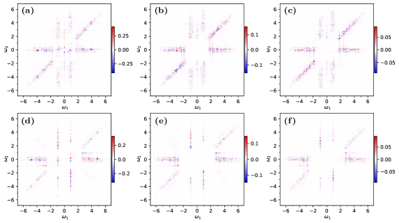
Figure 7: The difference between susceptibilities at two different finite sizes of system at the isotropic point with $K=0.2$. The top row shows the results $\chi^{(3),z}_{zzz}(\omega_{2},\omega_{1},0;L_{2})-\chi^{(3),z}_{zzz}(\omega_{2},\omega_{1},0;L_{1})$, for (a) $L_{2}=15,L_{1}=7$, (b) $L_{2}=27,L_{1}=15$ and (c) $L_{2}=33,L_{1}=27$. As the size of system is increased the difference of susceptibility at two successive sizes is reduced strongly. The bottom row exhibits similar results for $\chi^{(3),z}_{zzz}(\omega_{2},0,\omega_{1};L_{2})-\chi^{(3),z}_{zzz}(\omega_{2},0,\omega_{1};L_{1})$, where $L_{2}$ and $L_{1}$ are respectively (d) $15,7$, (e) $27,15$ and (f) $33,27$. Some streak signals can be seen in the above plots. Although these signals are present in the response of Fig. 3 they are so weak that are revealed only by subtracting the response at two successive system sizes.

Appendix C Finite size effects

Here, we show that the finite size effects in the nonlinear responses are weak and a system size of $33\times 33$ unit cells ($2178$ spins) represent a reasonable result for the nonlinear susceptibilities in the thermodynamic limit. The top row of Fig. 7 show the difference value of the normalized susceptibility $\chi^{(3),z}_{zzz}(\omega_{2},\omega_{1},0;L)$ for two different sizes. Fig. 7-(a) represents the difference $\chi^{(3),z}_{zzz}(\omega_{2},\omega_{1},0;L=15)-\chi^{(3),z}_{zzz}(\omega_{2},\omega_{1},0;L=7)$ and similar results have been plotted in (b) for $L=27,15$ and (c) for $L=33,27$. The color bar shows a decrease in the absolute value as the size increases, which justifies our claim. Similar values have been plotted in the bottom row of Fig. 7 for $\chi^{(3),z}_{zzz}(\omega_{2},0,\omega_{1};L)$, where (d) shows the results for $L=15,7$, (e) for $L=27,15$ and (f) for $L=33,27$. The weak finite size effect is expected since the underlying system is gapped.

Appendix D Response function versus exchange coupling

In order to further confirm our statement about the presence/absence of the streak signals in the Abelian phase of our model (cf. the last part of Sec. IV.1), we have plotted the nonlinear susceptibility in Fig. 8 for several values of $J$ along the white path shown in Fig. 5-(b). In these plots, $J=\frac{J_{y}}{J_{x}}=\frac{J_{z}}{J_{x}}$, and $K=0.2$, the top panel shows $\chi^{(3),z}_{zzz}(\omega_{2},\omega_{1},0)$ and the bottom panel represents $\chi^{(3),z}_{zzz}(\omega_{2},0,\omega_{1})$.It has to be mentioned that the plots in Fig. 8 represent unnormalized data that are indicated by their corresponding color bar, which shows the evolution of the response function with respect to $J$. The plots for $J=0.05$ show sharp spots revealing the contribution from a single excitation, while the plots for $J=0.25,0.45$ represent streak signals of several excitation modes. For the finite size of the underlying lattice $L_{1}=L_{2}=28$, the plots of $J=0.65$ show the crossover from the streak signals to sharp peaks of the flux excitations in non-Abelian phase, where the latter become obvious for $J=0.85$.

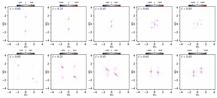
Figure 8: The top and bottom panels show susceptibilities $\chi^{(3),z}_{zzz}(\omega_{2},\omega_{1},0)$ and $\chi^{(3),z}_{zzz}(\omega_{2},0,\omega_{1})$, respectively. They are unnormalized 2D nonlinear response for several values of $J=0.05,0.25,0.45,0.65,0.85$ along the white path of Fig. 5-(b). In all plots the lattice geometry is $L_{1}=L_{2}=28$ and $M=0$.

Appendix E Effective Hamiltonian

Let us consider an extreme limit and assume $J_{x}=J_{y}=K=0$ in the EKM. For $J_{z}>0$, the spin configurations in which two spins on the z-link are aligned up or down ($|\uparrow\uparrow\rangle$ or $|\downarrow\downarrow\rangle$), form the degenerate ground state subspace with the energy $E_{0}=-NJ_{z}$. The two dimensional ground state subspace (on each z-link) can be considered as an effective spin $|\Uparrow\rangle$ or $|\Downarrow\rangle$ on the lattice, which is shown in Fig. 9-(b). The effective Pauli matrices act on the effective spins as sketched in Fig. 9-(c). For nonzero values of $J_{x},J_{y}$ and $K$, and in a perturbative regime where $J_{x},J_{y},K\ll J_{z}$, the Hamiltonian of the system is written as $H=H_{0}+V$,

$$H_{0}=-J_{z}\sum_{\text{i}\in\text{ z-links}}T^{z}_{i},\quad\quad V=-J_{x}\sum_{\text{i}\in\text{ x-links}}T^{x}_{i}-J_{y}\sum_{\text{i}\in\text{ y-links}}T_{i}^{y}-K\sum_{\begin{subarray}{c}\langle ik\rangle_{\alpha},\langle kj\rangle_{\beta}\\ \gamma\perp\alpha,\beta\end{subarray}}\hat{\sigma}^{\alpha}_{i}\hat{\sigma}^{\gamma}_{k}\hat{\sigma}^{\beta}_{j},$$ (55)

where $T^{\alpha}_{i}=\hat{\sigma}^{\alpha}_{k}\hat{\sigma}^{\alpha}_{j}$. The three-spin interactions can also be written in terms of $T_{i}^{\alpha}$’s. For instance, consider the plaquette $p_{1}$ in Fig. 9-(a), where all possible three-spin interactions are expressed in the following,

$$-K (\hat{\sigma}^{x}_{1}\hat{\sigma}^{z}_{2}\hat{\sigma}^{y}_{3}+\hat{\sigma}^{y}_{2}\hat{\sigma}^{x}_{3}\hat{\sigma}^{z}_{4}+\hat{\sigma}^{z}_{3}\hat{\sigma}^{y}_{4}\hat{\sigma}^{x}_{5}+\hat{\sigma}^{x}_{4}\hat{\sigma}^{z}_{5}\hat{\sigma}^{y}_{6}+\hat{\sigma}^{y}_{5}\hat{\sigma}^{x}_{6}\hat{\sigma}^{z}_{1}+\hat{\sigma}^{z}_{6}\hat{\sigma}^{y}_{1}\hat{\sigma}^{x}_{2})$$

$$=iK([T_{1}^{x}T_{2}^{y}]+[T_{2}^{y}T_{R}^{z}]+[T_{R}^{z}T_{3}^{x}]+[T_{3}^{x}T_{4}^{y}]+[T_{4}^{y}T_{L}^{z}]+[T_{L}^{z}T_{1}^{x}]),$$ (56)

where we used the square brackets to indicate the distinction between three-spin interaction terms and the interactions in the first and second terms of $V$. Suppose that $P_{0}$ and $Q_{0}$ are the projection operators onto the ground state subspace and excited states of $H_{0}$, respectively. By using the Brillouin-Wigner pertrurbaation approach the effective Hamiltonian of the system with energy $E\approx E_{0}$ is,

$$H_{\text{eff}}=P_{0}H_{0}P_{0}+P_{0}VP_{0}+P_{0}VG_{0}^{\prime}VP_{0}+P_{0}VG_{0}^{\prime}VG_{0}^{\prime}VP_{0}+\dots$$ (57)

where $G_{0}^{\prime}=\frac{1}{E_{0}-H_{0}}Q_{0}$ is the Green’s function.

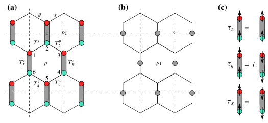
Figure 9: The strong links of EKM form an effective lattice in the large $J_{z}$ limit ($J_{z}\gg J_{x},J_{y},K$). (a) The large z-links are shown graphically with thick gray bonds and $T_{i}^{\alpha}$’s are Kitaev exchange interactions. (b) The gray circles represent the effective spins on the effective square lattice constructed with the dashed lines. (c) The act of effective Pauli operators on an effective spin is shown schematically.

The $n$-th order of perturbation term ($H_{\text{eff}}^{(n)}$) along with some of the interaction terms are given in the following,

$$H_{\text{eff}}^{(1)}=0$$ (58)

$$H_{\text{eff}}^{(2)}=\text{const.}-\frac{K^{2}}{2J_{z}}\sum_{i}Q_{p_{i}};\quad[T_{1}^{x}T_{2}^{y}][T_{3}^{x}T_{4}^{y}]\;\mbox{and}\;[T_{3}^{x}T_{4}^{y}][T_{1}^{x}T_{2}^{y}],$$ (59)

$$H_{\text{eff}}^{(3)}=\text{const.}-\left(\frac{J_{x}K^{2}}{4J_{z}^{2}}+\frac{J_{y}K^{2}}{4J_{z}^{2}}\right)\sum_{i}Q_{p_{i}};\quad[T_{3}^{x}T_{4}^{y}][T_{2}^{y}T_{R}^{z}]T_{1}^{x},\cdots,$$ (60)

$$H_{\text{eff}}^{(4)}=\text{const.}-\left(\frac{K^{4}+J_{x}^{2}K^{2}+J_{y}^{2}K^{2}+J_{x}^{2}J_{y}^{2}}{16J^{3}_{z}}\right)\sum_{i}Q_{p_{i}};\quad[T_{4}^{y}T_{L}^{z}][T_{R}^{z}T_{3}^{x}][T_{2}^{y}T_{R}^{z}][T_{L}^{z}T_{1}^{x}],[T_{4}^{y}T_{L}^{z}][T_{2}^{y}T_{R}^{z}]T_{3}^{x}T_{1}^{x},T_{4}^{y}T_{3}^{x}T_{2}^{y}T_{1}^{x},\dots,$$ (61)

where for example $Q_{p_{1}}=\hat{\sigma}_{2}^{z}\hat{\sigma}_{5}^{z}(\hat{\sigma}_{1}^{x}\hat{\sigma}_{6}^{y})(\hat{\sigma}_{3}^{y}\hat{\sigma}_{4}^{x})$ will be equal to $\hat{\tau}_{\text{up}}^{z}\hat{\tau}_{\text{down}}^{z}\hat{\tau}_{\text{left}}^{y}\hat{\tau}_{\text{right}}^{y}$ in terms of the effective Pauli matrices on the plaquette $p_{1}$ as shown in Fig. 9-(b)Kitaev (2006). Unlike the pure KM, the first nonzero term in the perturbation expansion appears at the second order since the three-spin interactions of the EKM are made up of two Kitaev interactions (E). With an appropriate unitary transformation, $H_{\text{eff}}$ in terms of $Q_{pi}$’s is transformed into the Kitaev toric codeKitaev (2006).

References

- Mila (2000) F. Mila, Eur. J. Phys. 21, 499 (2000).
- Balents (2010) L. Balents, Nature 464, 199 (2010).
- Savary and Balents (2017) L. Savary and L. Balents, Rep. Prog. Phys. 80, 016502 (2017).
- Zhou et al. (2017) Y. Zhou, K. Kanoda, and T.-K. Ng, Rev. Mod. Phys. 89, 025003 (2017).
- Knolle and Moessner (2019) J. Knolle and R. Moessner, Annu. Rev. Condens. Matter Phys. 10, 451 (2019).
- Broholm et al. (2020) C. Broholm, R. J. Cava, S. A. Kivelson, D. G. Nocera, M. R. Norman, and T. Senthil, Science 367, eaay0668 (2020).
- Wen (2007) X.-G. Wen, Quantum field theory of many-body systems (Oxford University Press, Oxford, 2007).
- Moessner and Moore (2021) R. Moessner and J. E. Moore, Topological Phases of Matter (Cambridge University Press, Cambridge, 2021).
- Sadrzadeh and Langari (2015) M. Sadrzadeh and A. Langari, Euro. Phys. J. B 88, 259 (2015).
- Sadrzadeh et al. (2016) M. Sadrzadeh, R. Haghshenas, S. S. Jahromi, and A. Langari, Phys. Rev. B 94, 214419 (2016).
- Sadrzadeh et al. (2019) M. Sadrzadeh, R. Haghshenas, and A. Langari, Phys. Rev. B 99, 144414 (2019).
- Anderson (1973) P. Anderson, Materials Research Bulletin 8, 153 (1973).
- Kitaev (2006) A. Kitaev, Annals of Physics 321, 2 (2006).
- Jackeli and Khaliullin (2009) G. Jackeli and G. Khaliullin, Phys. Rev. Lett. 102, 017205 (2009).
- Chaloupka et al. (2010) J. c. v. Chaloupka, G. Jackeli, and G. Khaliullin, Phys. Rev. Lett. 105, 027204 (2010).
- Plumb et al. (2014) K. W. Plumb, J. P. Clancy, L. J. Sandilands, V. V. Shankar, Y. F. Hu, K. S. Burch, H.-Y. Kee, and Y.-J. Kim, Phys. Rev. B 90, 041112 (2014).
- Winter et al. (2016) S. M. Winter, Y. Li, H. O. Jeschke, and R. Valentí, Phys. Rev. B 93, 214431 (2016).
- (18) S. Trebst, arXiv:1701.07056 .
- Winter et al. (2017a) S. M. Winter, A. A. Tsirlin, M. Daghofer, J. van den Brink, Y. Singh, P. Gegenwart, and R. Valentí, J. Phys.: Condens. Matter 29, 493002 (2017a).
- Takagi et al. (2019) H. Takagi, T. Takayama, G. Jackeli, G. Khaliullin, and S. E. Nagler, Nat. Rev. Phys. 1, 264 (2019).
- Liu (2021) H. Liu, Int. J. Mod. Phys. B 35, 2130006 (2021).
- Lahtinen et al. (2008) V. Lahtinen, G. Kells, A. Carollo, T. Stitt, J. Vala, and J. K. Pachos, Annals of Physics 323, 2286 (2008).
- Baskaran et al. (2007) G. Baskaran, S. Mandal, and R. Shankar, Phys. Rev. Lett. 98, 247201 (2007).
- Knolle et al. (2014a) J. Knolle, D. L. Kovrizhin, J. T. Chalker, and R. Moessner, Phys. Rev. Lett. 112, 207203 (2014a).
- Knolle et al. (2014b) J. Knolle, G.-W. Chern, D. L. Kovrizhin, R. Moessner, and N. B. Perkins, Phys. Rev. Lett. 113, 187201 (2014b).
- Knolle et al. (2015) J. Knolle, D. L. Kovrizhin, J. T. Chalker, and R. Moessner, Phys. Rev. B 92, 115127 (2015).
- Nasu et al. (2014) J. Nasu, M. Udagawa, and Y. Motome, Phys. Rev. Lett. 113, 197205 (2014).
- Perreault et al. (2015) B. Perreault, J. Knolle, N. B. Perkins, and F. J. Burnell, Phys. Rev. B 92, 094439 (2015).
- Halász et al. (2016) G. B. Halász, N. B. Perkins, and J. van den Brink, Phys. Rev. Lett. 117, 127203 (2016).
- Perreault et al. (2016) B. Perreault, J. Knolle, N. B. Perkins, and F. J. Burnell, Phys. Rev. B 94, 104427 (2016).
- Sandilands et al. (2015) L. J. Sandilands, Y. Tian, K. W. Plumb, Y.-J. Kim, and K. S. Burch, Phys. Rev. Lett. 114, 147201 (2015).
- Banerjee et al. (2016) A. Banerjee, C. A. Bridges, J.-Q. Yan, A. A. Aczel, L. Li, M. B. Stone, G. E. Granroth, M. D. Lumsden, Y. Yiu, J. Knolle, S. Bhattacharjee, D. L. Kovrizhin, R. Moessner, D. A. Tennant, D. G. Mandrus, and S. E. Nagler, Nat. Mater. 15, 733 (2016).
- Glamazda et al. (2016) A. Glamazda, P. Lemmens, S. H. Do, Y. S. Choi, and K.-Y. Choi, Nat. Commun. 7, 12286 (2016).
- Banerjee et al. (2017) A. Banerjee, J. Yan, J. Knolle, C. A. Bridges, M. B. Stone, M. D. Lumsden, D. G. Mandrus, D. A. Tennant, R. Moessner, and S. E. Nagler, Science 356, 1055 (2017).
- Wang et al. (2017) Z. Wang, S. Reschke, D. Hüvonen, S.-H. Do, K.-Y. Choi, M. Gensch, U. Nagel, T. Rõ om, and A. Loidl, Phys. Rev. Lett. 119, 227202 (2017).
- Banerjee et al. (2018) A. Banerjee, P. Lampen-Kelley, J. Knolle, C. Balz, A. A. Aczel, B. Winn, Y. Liu, D. Pajerowski, J. Yan, C. A. Bridges, A. T. Savici, B. C. Chakoumakos, M. D. Lumsden, D. A. Tennant, R. Moessner, D. G. Mandrus, and S. E. Nagler, Npj Quantum Mater. 3, 8 (2018).
- Wulferding et al. (2020) D. Wulferding, Y. Choi, S.-H. Do, C. H. Lee, P. Lemmens, C. Faugeras, Y. Gallais, and K.-Y. Choi, Nat. Commun. 11, 1603 (2020).
- Ruiz et al. (2021) A. Ruiz, N. P. Breznay, M. Li, I. Rousochatzakis, A. Allen, I. Zinda, V. Nagarajan, G. Lopez, Z. Islam, M. H. Upton, J. Kim, A. H. Said, X.-R. Huang, T. Gog, D. Casa, R. J. Birgeneau, J. D. Koralek, J. G. Analytis, N. B. Perkins, and A. Frano, Phys. Rev. B 103, 184404 (2021).
- Yang et al. (2022) Y. Yang, Y. Wang, I. Rousochatzakis, A. Ruiz, J. G. Analytis, K. S. Burch, and N. B. Perkins, Phys. Rev. B 105, L241101 (2022).
- Winter et al. (2017b) S. M. Winter, K. Riedl, P. A. Maksimov, A. L. Chernyshev, A. Honecker, and R. Valentí, Nat. Commun. 8, 1152 (2017b).
- Mukamel (1995) S. Mukamel, Principles of Nonlinear Optical Spectroscopy (Oxford University Press, New York, 1995).
- Mukamel (2000) S. Mukamel, Annu. Rev. Phys. Chem. 51, 691 (2000).
- Jonas (2003) D. M. Jonas, Annu. Rev. Phys. Chem. 54, 425 (2003).
- Cho (2008) M. Cho, Chem. Rev. 108, 1331 (2008).
- Hamm and Zanni (2011) P. Hamm and M. Zanni, Concepts and Methods of 2D Infrared Spectroscopy (Cambridge University Press, New York, 2011).
- Woerner et al. (2013) M. Woerner, W. Kuehn, P. Bowlan, K. Reimann, and T. Elsaesser, New J. Phys. 15, 025039 (2013).
- Cundiff and Mukamel (2013) S. T. Cundiff and S. Mukamel, Phys. Today 66, 44 (2013).
- Lu et al. (2017) J. Lu, X. Li, H. Y. Hwang, B. K. Ofori-Okai, T. Kurihara, T. Suemoto, and K. A. Nelson, Phys. Rev. Lett. 118, 207204 (2017).
- Cho (2019) M. Cho, ed., Coherent Multidimensional Spectroscopy (Springer, 2019).
- Wan and Armitage (2019) Y. Wan and N. P. Armitage, Phys. Rev. Lett. 122, 257401 (2019).
- Choi et al. (2020) W. Choi, K. H. Lee, and Y. B. Kim, Phys. Rev. Lett. 124, 117205 (2020).
- Nandkishore et al. (2021) R. M. Nandkishore, W. Choi, and Y. B. Kim, Phys. Rev. Research 3, 013254 (2021).
- Li et al. (2021) Z.-L. Li, M. Oshikawa, and Y. Wan, Phys. Rev. X 11, 031035 (2021).
- Phuc and Trung (2021) N. T. Phuc and P. Q. Trung, Phys. Rev. B 104, 115105 (2021).
- Fava et al. (2021) M. Fava, S. Biswas, S. Gopalakrishnan, R. Vasseur, and S. A. Parameswaran, Proc. Natl. Acad. Sci. USA 118, e2106945118 (2021).
- Mahmood et al. (2021) F. Mahmood, D. Chaudhuri, S. Gopalakrishnan, R. Nandkishore, and N. P. Armitage, Nat. Phys. 17, 627 (2021).
- (57) O. Hart and R. Nandkishore, arXiv:2208.12817 .
- (58) M. Fava, S. Gopalakrishnan, R. Vasseur, F. H. L. Essler, and S. A. Parameswaran, arXiv:2208.09490 .
- Parameswaran and Gopalakrishnan (2020) S. A. Parameswaran and S. Gopalakrishnan, Phys. Rev. Lett. 125, 237601 (2020).
- (60) G. Sim, J. Knolle, and F. Pollmann, arXiv:2209.00720 .
- (61) Q. Gao, Y. Liu, H. Liao, and Y. Wan, arXiv:2209.14070 .
- Kanega et al. (2021) M. Kanega, T. N. Ikeda, and M. Sato, Phys. Rev. Research 3, L032024 (2021).
- Holleis et al. (2021) L. Holleis, J. C. Prestigiacomo, Z. Fan, S. Nishimoto, M. Osofsky, G.-W. Chern, J. van den Brink, and B. S. Shivaram, Npj Quantum Mater. 6, 66 (2021).
- (64) M. McGinley, M. Fava, and S. A. Parameswaran, arXiv:2210.16249 .
- Pedrocchi et al. (2011) F. L. Pedrocchi, S. Chesi, and D. Loss, Phys. Rev. B 84, 165414 (2011).
- Blaizot and Ripka (1985) J. P. Blaizot and G. Ripka, Quantum Theory Of Finite Systems (MIT Press, Cambridge, 1985).
- Yao et al. (2009) H. Yao, S.-C. Zhang, and S. A. Kivelson, Phys. Rev. Lett. 102, 217202 (2009).
- Yao and Qi (2010) H. Yao and X.-L. Qi, Phys. Rev. Lett. 105, 080501 (2010).
- Halász et al. (2014) G. B. Halász, J. T. Chalker, and R. Moessner, Phys. Rev. B 90, 035145 (2014).
- Lieb (1994) E. H. Lieb, Phys. Rev. Lett. 73, 2158 (1994).
- Zschocke and Vojta (2015) F. Zschocke and M. Vojta, Phys. Rev. B 92, 014403 (2015).
- Kells et al. (2009) G. Kells, J. K. Slingerland, and J. Vala, Phys. Rev. B 80, 125415 (2009).
- Nayak et al. (2008) C. Nayak, S. H. Simon, A. Stern, M. Freedman, and S. Das Sarma, Rev. Mod. Phys. 80, 1083 (2008).
- (74) We computed fast fourier transformation with Python package for calculation two-dimensional discrete fast fourier transformation.
- Lahtinen (2011) V. Lahtinen, New J. Phys. 13, 075009 (2011).