A modular framework for stabilizing deep reinforcement learning control

Abstract

We propose a framework for the design of feedback controllers that combines the optimization-driven and model-free advantages of deep reinforcement learning with the stability guarantees provided by using the Youla-Kučera parameterization to define the search domain. Recent advances in behavioral systems allow us to construct a data-driven internal model; this enables an alternative realization of the Youla-Kučera parameterization based entirely on input-output exploration data. Using a neural network to express a parameterized set of nonlinear stable operators enables seamless integration with standard deep learning libraries. We demonstrate the approach on a realistic simulation of a two-tank system.

1 Introduction

Closed-loop stability is a basic requirement in controller design. However, many learning-based control schemes do not address it explicitly (Buşoniu et al., 2018). This is somewhat understandable. First, the “model-free” setup assumed in such algorithms, compounded by the complexity of the methods and their underlying data structures, makes stability difficult to reason about. Second, especially in the case of reinforcement learning (RL), many of the striking recent success stories pertain to simulated tasks or game-playing environments in which catastrophic failure has no real-world impact. When the feedback controller is to be learned directly with RL, tuning the discount factor and/or the reward function influences not only the learning performance but also the stability during exploration (Buşoniu et al., 2018). This issue provides a counterpoint to the generality and expressive capacity of modern RL algorithms, which have nonetheless attracted immense interest for control tasks (Nian et al., 2020).

In this work, we propose a stability-preserving framework for RL-based controller design. Our inspiration is the Youla-Kučera  parameterization (Anderson, 1998), which gives a characterization of all stabilizing controllers for a given system. The key design variable is then a stable “parameter”, rather than a direct controller representation. Optimizing over stable operators is still non-trivial, but we show how this can be done in a flexible manner using neural networks. Finally, the Youla-Kučera parameterization requires an internal model of the system, which contradicts one of the key advantages of RL. We address this with tools from the behavioral systems literature (Markovsky and Dörfler, 2021), specifically, Willems’ fundamental lemma (Willems et al., 2005). This powerful result provides a characterization of system dynamics entirely from input-output data. We leverage this to yield a “model-free” internal representation for the plant, resulting in a mathematically equivalent realization of the Youla-Kučera  parameterization.

In sum, we disentangle three key components in RL-based control system design: algorithms, function approximators, and dynamic models. The resulting framework supports a modular approach to learning stabilizing policies, in which advances in any single category can be applied to improve overall results.

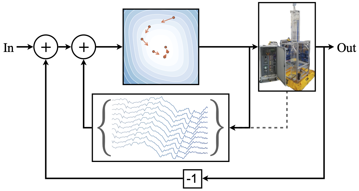
Figure 1: A stable nonlinear parameter $Q$ interacts with its environment; collected input-output trajectories are used to construct a Hankel matrix. These ingredients yield an equivalent realization of the Youla-Kučera parameterization.

1.1 Related work

Buşoniu et al. (2018) provide a survey of RL techniques from a control-theoretic perspective, emphasizing the need for stability-aware RL algorithms. Existing strategies for incorporating stability into RL can be described in three broad categories: integral quadratic constraints (IQCs), Lyapunov’s second method, and the Youla-Kučera  parameterization.

IQCs are a method from robust control theory for proving stability of a dynamical system with some nonlinear or time-varying component. In the context of RL, nonlinearities in the environment or the nonlinear activation functions used to compose a policy neural network can be characterized using IQCs. This has been the approach in several recent works, for example, Jin and Lavaei (2020); Wang et al. (2022).

Lyapunov stability theory is also well represented in the RL literature (Berkenkamp et al., 2017; Han et al., 2020). The principal idea is to learn a policy that guarantees the steady decrease of a suitable Lyapunov function. Berkenkamp et al. (2017) proposed one of the first methods to establish stability with deep neural network policies: a Lyapunov function and a statistical model of the environment are assumed to be available, then the policy is optimized within an expanding estimate of the region of attraction. Subsequent works add the task of acquiring a Lyapunov function to the learning process (Lawrence et al., 2020). For example, Han et al. (2020) exploit a trainable Lyapunov neural network in tandem with the policy. Methods based on merging model predictive control with RL (Zanon and Gros, 2020) also make essential use of Lyapunov analysis.

The Youla-Kučera  parameterization is a seemingly under-utilized technique for integrating stability into RL algorithms. Friedrich and Buss (2017) employ the Youla-Kučera  parameterization through the use of a crude plant model; RL is used to optimize the tracking performance of a physical two degree of freedom robot in a safe fashion while accounting for unmodeled nonlinearities. Recently, a recurrent neural network architecture based on IQCs was developed (Revay et al., 2021). Since this architecture satisfies stability conditions by design, it can be used for control in a nonlinear version of the Youla-Kučera  parameterization (Wang et al., 2022).

While we also use the Youla-Kučera  parameterization, our approach has several novel aspects. Its method for producing stable operators uses a non-recurrent neural network structure; this makes the implementation and integration with off-the-shelf RL algorithms relatively straightforward, for both on-policy and off-policy learning. We also formulate a data-driven realization of the Youla-Kučera  parameterization based on Willems’ fundamental lemma, essentially removing the prior modeling assumption.

2 Background

This section lays out the foundational pieces for our approach. We first connect Willems’ lemma to the Youla-Kučera parameterization, then we show our approach to learning stable operators.

We consider linear time-invariant (LTI) systems of the form

$$\begin{split}x_{t+1}&=Ax_{t}+Bu_{t}\\ y_{t}&=Cx_{t}+Du_{t}\end{split}$$ (1)

Sometimes it is convenient to express Equation 1 as a transfer function, in which case we write $P=P(z)=C(zI-A)^{-1}B+D$. We assume that $(A,B)$ is controllable, that $(A,C)$ is observable, and that an upper bound of the order of the system is known. Crucially, the system matrices are unknown. For simplicity in our formulation we assume the system of interest is stable and single-input single-output, however, the results can be extended to more general cases.

2.1 Data-driven realization of the Youla-Kučera parameterization

Given an $N$-element sequence $\{z_{t}\}_{t=0}^{N-1}$ of vectors in $\mathbb{R}^{m}$, the Hankel matrix of order $L$ is given by

$$H_{L}(z)=\begin{bmatrix}z_{0}&z_{1}&\ldots&z_{N-L}\\ z_{1}&z_{2}&\ldots&z_{N-L+1}\\ \vdots&\vdots&\ddots&\vdots\\ z_{L-1}&z_{L}&\ldots&z_{N-1}\end{bmatrix}.$$

Definition 2.1

The sequence $\{z_{t}\}_{t=0}^{N-1}\subset\mathbb{R}^{m}$ is persistently exciting of order $L$ if $\operatorname{rank}(H_{L}(z))=mL$.

Definition 2.2

An input-output sequence $\{u_{t},y_{t}\}_{t=0}^{N-1}$ is a trajectory of an LTI system $(A,B,C,D)$ if there exists a state sequence $\{x_{t}\}_{t=0}^{N-1}$ such that Equation 1 holds.

The following theorem is the state-space version of Willems’ fundamental lemma (Willems et al., 2005). It provides an alternative characterization of an LTI system based entirely on input-output data. Only an upper bound of the order of the system is required.

Theorem 2.3 (See van Waarde et al. (2020))

Let $\{u_{t},y_{t}\}_{t=0}^{N-1}$ be a trajectory of an LTI system $(A,B,C,D)$ where $u$ is persistently exciting of order $L+n$. Then $\{\overline{u}_{t},\overline{y}_{t}\}_{t=0}^{L-1}$ is a trajectory of $(A,B,C,D)$ if and only if there exists $\alpha\in\mathbb{R}^{N-L+1}$ such that

$$\begin{bmatrix}H_{L}(u)\\ H_{L}(y)\end{bmatrix}\alpha=\begin{bmatrix}\overline{u}\\ \overline{y}\end{bmatrix}.$$ (2)

(When we omit the time index in the context of the right-hand side of Equation 2, it is understood as a column vector $\overline{z}=[\overline{z}_{0}\ldots\overline{z}_{L-1}]^{T}$. ) Equation 2 has been applied extensively for predictive control tasks (Markovsky and Dörfler, 2021; Berberich and Allgower, 2020). In particular, a sequence of inputs may be proposed, and through a slight variation of Equation 2, the corresponding outputs computed. This leads to a scheme of forecasting a sequence of inputs and “filling in” the outputs.

In what follows, we consider the scenario of using the Hankel based model as an internal system model. Therefore, we assume the system is strictly proper — that is, $D=0$ in Equation 1 — to ensure a realizable controller strategy later on. Now, given a system trajectory $\{u_{t},y_{t}\}_{t=0}^{L-1}$, we note that $y_{L}$ is uniquely determined by these available data. A simple way of stepping the system forward is to consider a time-shifted Hankel matrix

$$H^{\prime}_{L}(z)=H_{L}(z^{\prime}),$$

where $z=\{z_{t}\}_{t=0}^{N-1}$ and $z^{\prime}=\{z_{t}\}_{t=1}^{N}$ for some $N$.

Corollary 2.4

Let $\{u_{t},y_{t}\}_{t=0}^{N-1}$ be a trajectory of a strictly proper LTI system $(A,B,C)$ where $u$ is persistently exciting of order $L+n+1$. Then for each trajectory $\{\overline{u}_{t},\overline{y}_{t}\}_{t=0}^{L-1}$ of $(A,B,C)$, there exists $\alpha\in\mathbb{R}^{N-L}$ such that

$$\overline{y}^{\prime}=H^{\prime}_{L}(y)\alpha.$$

By Equation 2, the trajectory $\{\overline{u}_{t},\overline{y}_{t}\}_{t=0}^{L-1}$ satisfies

$$\begin{bmatrix}H_{L}(u)\\ H_{L}(y)\end{bmatrix}\alpha=\begin{bmatrix}\overline{u}\\ \overline{y}\end{bmatrix}$$

for some $\alpha\in\mathbb{R}^{N-L}$. Moreover, by Definition 2.2 there exists a sequence of states $\{\overline{x}_{t}\}_{t=0}^{L-1}$ that corresponds to the input-output trajectory $\{\overline{u}_{t},\overline{y}_{t}\}_{t=0}^{L-1}$. This sequence induces the state $\overline{x}_{L}$. We have

$$\overline{y}_{L} =C\overline{x}_{L}$$

$$=C\left(A\overline{x}_{L-1}+B\overline{u}_{L-1}\right)$$

$$=C\left(A\sum_{i=0}^{N-L-1}\alpha_{i}x_{L+i}+B\sum_{i=0}^{N-L-1}\alpha_{i}u_{L+i}\right)$$

$$=\sum_{i=0}^{N-L-1}\alpha_{i}C\left(Ax_{L+i}+Bu_{L+i}\right)$$

$$=\sum_{i=0}^{N-L-1}\alpha_{i}y_{L+i+1}$$

as desired. ∎

Corollary 2.4 gives a systematic way of stepping a trajectory forward in time. This is particularly useful for aligning the true system with a Hankel representation while implementing a feedback controller online.

The Youla-Kučera  parameterization produces the set of all stabilizing controllers through a combination of an internal system model and a stable operator. The trick is to directly parameterize the closed-loop transfer functions associated with the plant, then recover a controller. For example, the behavior of the closed-loop transfer function $\frac{PC}{1+PC}$ from the reference $r$ to output $y$ is determined by the transfer function $\frac{C}{1+PC}$. By introducing a stable design variable $Q$, we can then directly shape the stable behavior of the system through the transfer function $PQ$. By setting $Q=\frac{C}{1+PC}$, we arrive at the Youla-Kučera  parameterization (Anderson, 1998):

$$\mathcal{C}_{\text{stable}}=\left\{\frac{Q}{1-QP}\colon Q\text{ is stable}\right\}$$

This result extends further to unstable, multiple-input multiple-output systems. Moreover, when $P$ is linear, one may use a nonlinear operator $Q$ (Anderson, 1998).

In Algorithm 1, we translate the mathematical ideas above into a direct sequential process. The following result provides details of the correspondence.

Theorem 2.5

Assume $P$ is a stable and strictly proper LTI system. Let $Q$ be a stable and proper LTI parameter. Given an upper bound $L$ of the order of $P$, Algorithm 1 produces the same control signal $\{\overline{u}_{t}\}_{t=0}^{\infty}$ as the Youla-Kučera  parameterization.

We use $q_{t}$, $p_{t}$ to denote the impulse responses of $Q$ and $P$, respectively. Similarly, respective minimal state-space matrices are denoted $(A_{q},B_{q},C_{q},D_{q})$ and $(A_{p},B_{p},C_{p})$.

By the Youla-Kučera  parameterization, we have

$$C(z) =\frac{Q(z)}{1-Q(z)P(z)}\quad\forall z\in\mathbb{C}$$

$$\iff \left(1-Q(z)P(z)\right)U(z) =Q(z)E(z)$$

$$\iff u_{t} =q_{t}*(e_{t}+p_{t}*u_{t})\quad\forall t\in\mathbb{N}_{0}$$

$$=\sum_{j=0}^{t-1}C_{q}A_{q}^{t-1-j}B_{q}\widehat{r}_{j}+D_{q}\widehat{r}_{t},$$ (3)

where $\widehat{r}_{j}=e_{j}+\sum_{i=0}^{j-1}C_{p}A_{p}^{j-1-i}B_{p}u_{i}$ and $*$ is the convolution operator; we have also assumed, without loss of generality, that $P$ and $Q$ have zero initial state.

Next we relate Equation 3 to Algorithm 1. Let $\{e_{k}\}_{k=0}^{\infty}$ be an arbitrary sequence. (Such a sequence is dynamically generated in Algorithm 1.) Without loss of generality, let the initial trajectory be $\{\overline{u}_{k},\overline{y}_{k}\}_{k=0}^{L-1}=\{0,0\}_{k=0}^{L-1}$. For each time $t\in\mathbb{N}_{0}$ we compute $\alpha^{(t)}$ and $\overline{y}_{t}=\overline{y}_{L}$ from Corollary 2.4. Since $L$ is an upper bound of the order of $P$, $\overline{y}_{t}$ is the unique next output from the trajectory $\{\overline{u}_{k},\overline{y}_{k}\}_{k=0}^{L-1}$. Therefore, we have

$$\widehat{r}_{t}=e_{t}+\sum_{i=0}^{N-L-1}\alpha_{i}^{(t)}y_{L+i+1}.$$

Then

$$\overline{u}_{t}=\sum_{j=0}^{t-1}C_{q}A_{q}^{t-1-j}B_{q}\widehat{r}_{j}+D_{q}\widehat{r}_{t}$$

gives the next control input.

By updating the trajectory between time steps — $\{\overline{u}_{k},\overline{y}_{k}\}_{k=0}^{L-1}\leftarrow\{\overline{u}_{k},\overline{y}_{k}\}_{k=1}^{L}$ — we dynamically generate a sequence $\{\alpha^{(t)}\}_{t=0}^{\infty}$ that produces the control inputs $\{\overline{u}_{t}\}_{t=0}^{\infty}$ satisfying the discrete integral equation in Equation 3. ∎

Algorithm 1 Data-driven stabilizing controller

1:Input: Stable $Q$ parameter; Observations $\{u_{k},y_{k}\}_{k=0}^{N-1}$; Initial trajectory $\{\overline{u}_{k},\overline{y}_{k}\}_{k=0}^{L-1}$

2:for each time step $t$ do

3:     Set $u_{t-1}\leftarrow\overline{u}_{L-1}$

4:     Observe the tracking error $e_{t}=r_{t}-y_{t}$

5:     Compute $\overline{y}_{L}$ from Corollary 2.4

6:     Apply the input $\widehat{r}=e_{t}+\overline{y}_{L}$ to the $Q$ parameter and return control action $u_{L}$

7:     Update trajectory:

$$\{\overline{u}_{k},\overline{y}_{k}\}_{k=0}^{L-1}\leftarrow\{\overline{u}_{k},\overline{y}_{k}\}_{k=1}^{L}$$

2.2 Learning stable operators

The Youla-Kučera  parameterization is very elegant, as it refines the search space for any problem to the set of stable operators. However, effectively optimizing over this set is still a major challenge (Wang et al., 2022).

We adapt the method due to Lawrence et al. (2020). First let us recall the notion of a Lyapunov candidate function $V\colon\mathbb{R}^{n}\to\mathbb{R}$: 1) $V$ is continuous; 2) $V(z)>0$ for all $z\neq 0$, and $V(0)=0$; 3) There exists a continuous, strictly increasing function $\varphi\colon[0,\infty)\to[0,\infty)$ such that $V(z)\geq\varphi(\mathchoice{\left\|{{{{z}}}}\right\|}{\|{{{{z}}}}\|}{\|{{{{z}}}}\|}{\|{{{{z}}}}\|})$ for all $z\in\mathbb{R}^{n}$; 4) $V(z)\to\infty$ as $\mathchoice{\left\|{{{{z}}}}\right\|}{\|{{{{z}}}}\|}{\|{{{{z}}}}\|}{\|{{{{z}}}}\|}\to\infty$.

Lyapunov functions are instrumental for proving a system is stable through Lyapunov’s second method (Khalil, 2002). Lawrence et al. (2020) construct stable autonomous systems of the form $z_{t+1}=f_{\theta}(z_{t})$ “by design” through the use of trainable Lyapunov functions. A neural network satisfying the principal requirements above can be obtained through a slightly modified input-convex neural network (Amos et al., 2017) — see Lawrence et al. (2020) and the references therein for details.

Two neural networks work in tandem to form a single model that satisfies the decrease condition central to Lyapunov’s second method: a smooth neural network $\widehat{f}_{\theta}$, and a Lyapunov neural network $V_{\theta}$. Set $\widehat{z}^{\prime}=\widehat{f}_{\theta}(z)$ where $z$ is the current state and $\widehat{z}^{\prime}$ is the proposed next state. Two cases are possible: either $\widehat{z}^{\prime}$ decreased the value of $V$ or it did not. We can write out a “correction” to the dynamics in closed form by exploiting the convexity of $V$:

$$\begin{split}z_{t+1}&=f_{\theta}(z_{t})\\ &\equiv\begin{cases}\widehat{f}_{\theta}(z_{t}),&\text{if }V(\widehat{f}_{\theta}(z_{t}))\leq\beta V(z_{t})\\ \widehat{f}_{\theta}(z_{t})\left(\frac{\beta V(z_{t})}{V(\widehat{f}_{\theta}(z_{t}))}\right),&\text{otherwise}\end{cases}\\ &=\gamma\widehat{f}_{\theta}(z_{t}),\text{ where}\\ \ &\gamma=\gamma(z_{t})=\frac{\beta V(z_{t})-\texttt{ReLU}\big{(}\beta V(z_{t})-V(\widehat{f}_{\theta}(z_{t}))}{V(\widehat{f}_{\theta}(z_{t}))}.\end{split}$$ (4)

Since Equation 4 defines the model $f_{\theta}$, both $\widehat{f}_{\theta}$ and $V_{\theta}$ are trained in unison towards whatever goal is required of the sequential states $z_{t},z_{t+1},\ldots$, such as supervised learning tasks. Moreover, although the model $f_{\theta}$ is constrained to be stable, it is unconstrained in parameter space, making its implementation and training fairly straightforward with deep learning libraries. Further, despite the complex structure in Equation 4, Lawrence et al. (2020) show that the overall model is continuous. Here, we use $f_{\theta}$ to model the internal dynamics of a nonlinear $Q$ parameter. For example, a control–affine model may be used with stable transition dynamics $f_{\theta}$.

3 Unconstrained stabilizing reinforcement learning

A brief overview of deep RL will serve to define our notation, which is largely standard. For more background, see Sutton and Barto (2018); Buşoniu et al. (2018); a tutorial-style treatment is given by Nian et al. (2020).

Reinforcement learning is an optimization-driven framework for learning “policies” simply through interactions with an environment (Sutton and Barto, 2018). The states $s$ and actions $a$ belong to the state and action sets $\mathcal{S}$, $\mathcal{A}$, respectively. At each time step $t$, the state $s_{t}$ influences the sampling of an action $a_{t}\sim\pi(\cdot\mid s_{t})$ from the “policy” $\pi$. Given the action $a_{t}$, the environment produces a successor state $s_{t+1}$. This cycle completes one step in a Markov decision process, which induces a conditional density function $s_{t+1}\sim p(\cdot\mid s_{t},a_{t})$ for any initial distribution $s_{0}\sim p_{0}(\cdot)$. As time steps forward under a policy $\pi$, a “rollout” is denoted $h=(s_{0},a_{0},r_{0},s_{1},a_{1},r_{1},\ldots)$. Each fixed policy $\pi$, induces a probability density $p^{\pi}(\cdot)$ on the set of trajectories.

In RL the desirability of a given rollout is quantified by a “reward” $r_{t}=r(s_{t},a_{t})$ associated with each stage in the process above. The overall goal of the agent is to determine a policy that maximizes the cumulative discounted reward. That is, given some constant $\gamma\in(0,1)$,

maximize $$J(\pi)=\mathbb{E}_{h\sim p^{\pi}}\left[\sum_{t=0}^{\infty}\gamma^{t}r(s_{t},a_{t})\right]$$ (5)

over all $$\text{policies }\pi\colon\mathcal{S}\to\mathcal{P}(\mathcal{A}),$$

where $\mathcal{P}(\mathcal{A})$ denotes the set of probability measures on $\mathcal{A}$.

In the space of all possible policies, the optimization is performed over a subset parameterized by some vector $\theta$. For example, in some applications, $\theta$ denotes the set of all weights in a deep neural network. In this work, the policy is the nonlinear $Q$ parameter outlined in Section 2.2. Therefore, Equation 5 automatically satisfies an internal stability constraint over the whole weight space $\theta$. We are then able to use any RL algorithm to solve the problem. We do not recount the inner workings of common RL algorithms, as they are well-documented (Nian et al., 2020). Instead, a brief overview is given.

The broad subject of reinforcement learning concerns iterative methods for choosing a desirable policy $\pi$ (this is the “learning”), guided in some fundamental way by the agent’s observations of the rewards from past state-action pairs (this provides the “reinforcement”).

A standard approach to solving Problem (5) uses gradient ascent

$$\theta\leftarrow\theta+\alpha\nabla J(\theta),$$

where $\alpha>0$ is a step-size parameter. Analytic expressions for $\nabla J(\theta)$ exist for both stochastic and deterministic policies (see Sutton and Barto (2018); Buşoniu et al. (2018)). Crucially, these formulas rely on the state-action value function,

$$Q^{(\text{RL})}(s_{t},a_{t})=\mathbb{E}_{h\sim p^{\pi}}\left[\sum_{k=t}^{\infty}\gamma^{k-t}r(s_{k},a_{k})\middle|s_{t},a_{t}\right].$$

Although $Q^{(\text{RL})}$ is not known precisely, as it depends on both the dynamics and the policy, it can be estimated with a deep neural network (Buşoniu et al., 2018). These ideas and various approximation techniques form the basis of deep RL algorithms.

4 A simulation example

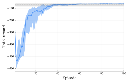
Figure 2: Cumulative reward curve over $20$ training sessions. The solid line is the median and the shaded region shows the interquartile range. The dashed line and its shaded region are the final results of training without the stability constraint.

We showcase our training results on a realistic simulation of a level-control system involving two large tanks of water. The objective is to regulate the water level in the upper tank, while water continuously drains out into a lower reservoir. A pump lifts water from the reservoir back to the upper tank, establishing a cyclic flow. A physical depiction of the setup is shown in Figure 1 and further explained in Lawrence et al. (2022).

The system dynamics are based on Bernoulli’s equation, establishing outflow $f_{\text{out}}\approx f_{c}\mathchoice{{\hbox{$\displaystyle\sqrt{2g\ell\,}$}\lower 0.4pt\hbox{\vrule height=6.94444pt,depth=-5.55559pt}}}{{\hbox{$\textstyle\sqrt{2g\ell\,}$}\lower 0.4pt\hbox{\vrule height=6.94444pt,depth=-5.55559pt}}}{{\hbox{$\scriptstyle\sqrt{2g\ell\,}$}\lower 0.4pt\hbox{\vrule height=4.8611pt,depth=-3.8889pt}}}{{\hbox{$\scriptscriptstyle\sqrt{2g\ell\,}$}\lower 0.4pt\hbox{\vrule height=3.47221pt,depth=-2.77779pt}}}$, and the conservation of fluid volume in the upper tank:

$$\frac{d\hfil}{dt}\left(\pi r_{\text{tank}}^{2}\ell\right)=\pi r_{\text{tank}}^{2}\dot{\ell}=f_{\text{in}}-f_{\text{out}}$$

(We use dot notation to represent differentiation with respect to time; $g$ is the gravitational constant; $\ell$ is the level; $r_{\text{tank}}$ is the radius of the tank; see Lawrence et al. (2022) for a more thorough description of the system.) Our application involves four filtered signals, with time constants $\tau_{p}$ for the pump, $\tau_{\text{in}}$ for changes in the inflow, $\tau_{\text{out}}$ for the outflow, and $\tau_{m}$ for the measured level dynamics. We therefore have the following system of differential equations describing the pump speed, flow rates, level, and measured level, respectively:

$$\tau_{p}\dot{p}+p =p_{\text{sp}}$$

$$\tau_{\text{in}}\dot{f}_{\text{in}}+f_{\text{in}} =f_{\text{max}}\left(\frac{p}{100}\right)$$

$$\tau_{\text{out}}\dot{f}_{\text{out}}+f_{\text{out}} =\pi r_{\text{pipe}}^{2}f_{\text{c}}\mathchoice{{\hbox{$\displaystyle\sqrt{2g\ell\,}$}\lower 0.4pt\hbox{\vrule height=6.94444pt,depth=-5.55559pt}}}{{\hbox{$\textstyle\sqrt{2g\ell\,}$}\lower 0.4pt\hbox{\vrule height=6.94444pt,depth=-5.55559pt}}}{{\hbox{$\scriptstyle\sqrt{2g\ell\,}$}\lower 0.4pt\hbox{\vrule height=4.8611pt,depth=-3.8889pt}}}{{\hbox{$\scriptscriptstyle\sqrt{2g\ell\,}$}\lower 0.4pt\hbox{\vrule height=3.47221pt,depth=-2.77779pt}}}$$

$$\pi r_{\text{tank}}^{2}\dot{\ell} =f_{\text{in}}-f_{\text{out}}$$

$$\tau_{m}\dot{m}+m =\ell$$

To track a desired level $\ell_{\text{sp}}$ — “sp” stands for “setpoint” — we can employ level and flow controllers by including the following equations:

$$\begin{split}p_{\text{sp}}&=\text{PID}_{\text{flow}}(f_{\text{in,sp}}-f_{\text{in}})\\ f_{\text{in,sp}}&=\text{PID}_{\text{level}}(\ell_{\text{sp}}-m)\end{split}$$ (6)

Equation 6 uses shorthand for PID controllers taking the error signals $f_{\text{in,sp}}-f_{\text{in}}$ and $\ell_{\text{sp}}-m$, respectively. For our purposes, $\text{PID}_{\text{flow}}$ and $\text{PID}_{\text{level}}$ are fixed and a part of the environment. The implementation of these dynamics is performed in discrete time steps of 0.5 seconds and with Gaussian measurement noise with variance $0.015$.

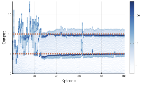
Figure 3: A global view of the training progress across all $20$ sessions. For each episode, a distribution of time spent at various output values is obtained. The heatmap shows the average amount of time spent at each episode–output coordinate.

(Training results) Since the environment includes a PID controller, we modify the control scheme to be in incremental form $u_{t}=u_{t-1}+\Delta u_{t}$, where $\Delta u_{t}$ is the sum of the Youla-Kučera  parameter and PID controller outputs:

$$\Delta u_{t}=\Delta u^{(q)}_{t}+\Delta u^{(\text{PID})}_{t}$$

We ran $20$ training sessions for $100$ episodes each and combined the results in Figures 2 and 3. Figure 2 shows the cumulative rewards for each episode. We convey the median and interquartile ranges over the $20$ training sessions; we see that median reward curve is much closer to the upper limit of the shaded region than the lower, indicating that the majority of experiments fall within that tight region. Although there is significant variation at initialization, due to the random policy initialization, the training sessions exhibit consistent convergence. The reward curves tend to plateau after around $40$ episodes.

Figure 3 shows the collective evolution of each episode throughout the training sessions. Each episode–output coordinate is shaded based on how much time the output variable spent there on average. Darker shading around the dashed values (setpoints) is more desirable. The purpose of this figure is to provide a rough translation of what the reward curve in Figure 2 entails. On the other hand, Figure 4 shows a single rollout from one of the experiments.

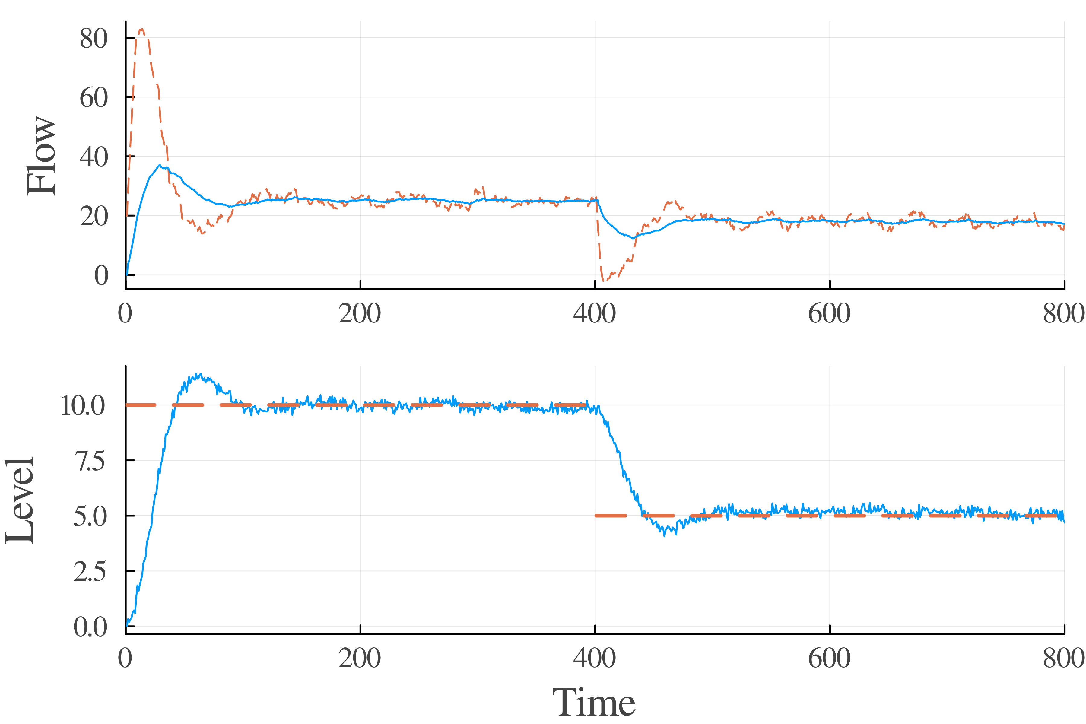
Figure 4: A sample input-output rollout by the trained RL agent for one of the training sessions. Dashed lines are setpoints; solid lines are measured values.

5 Conclusion

The Youla-Kučera  parameterization is well-known in control theory, but seemingly under-utilized in RL. Taking it as a starting point, we have adopted advances in deep learning and behavioral systems to develop an end-to-end framework for learning stabilizing policies with general RL algorithms. This paper is a proof of concept and there are many avenues to explore. These include the use of stochastic policies; extensions to unstable systems; and balancing the persistence of excitation assumption during training and steady-state operations. We believe this is a fruitful area to investigate further as deep RL gains traction in process systems engineering.

We gratefully acknowledge the financial support of the Natural Sciences and Engineering Research Council of Canada (NSERC) and Honeywell Connected Plant. We would also like to thank Professor Yaniv Plan for helpful discussions.

Appendix A Implementation details

Numerical experiments were carried out in the Julia programming language. In particular, we utilized the ReinforcementLearning.jl package (Tian and contributors, 2020). We used the TD3 algorithm (Fujimoto et al., 2018) to update network parameters. We used the reward function $-0.1\mathchoice{\left|{{{{y_{\text{sp}}-y}}}}\right|}{|{{{{y_{\text{sp}}-y}}}}|}{|{{{{y_{\text{sp}}-y}}}}|}{|{{{{y_{\text{sp}}-y}}}}|}-0.01\left(\Delta u^{(q)}\right)^{2}$. Most hyperparameters were set to their default values; we set the policy delay to $4$. We used two-layer feedforward networks throughout. The critic network had $64$ nodes per layer and used the softplus activation. We used the same structure for the actor in the stability-free comparison shown in Figure 2. For the stable $Q$ parameter we used Equation 4 and created a state-space model with matrices $B,C,D$ and $f_{\theta}$ instead of the nominal $A$ matrix. $\widehat{f}_{\theta}$ had $16$ nodes per layer and used the tanh activation. $V_{\theta}$ also had $16$ nodes per layer.

References

- Amos et al. (2017) Amos, B., Xu, L., and Kolter, J.Z. (2017). Input convex neural networks. In Proceedings of the 34th International Conference on Machine Learning, volume 70 of Proceedings of Machine Learning Research, 146–155. PMLR. URL https://proceedings.mlr.press/v70/amos17b.html.
- Anderson (1998) Anderson, B.D. (1998). From Youla–Kucera to identification, adaptive and nonlinear control. Automatica, 34(12), 1485–1506. 10.1016/S0005-1098(98)80002-2.
- Berberich and Allgower (2020) Berberich, J. and Allgower, F. (2020). A trajectory-based framework for data-driven system analysis and control. In 2020 European Control Conference (ECC), 1365–1370. IEEE, Saint Petersburg, Russia. 10.23919/ECC51009.2020.9143608.
- Berkenkamp et al. (2017) Berkenkamp, F., Turchetta, M., Schoellig, A., and Krause, A. (2017). Safe model-based reinforcement learning with stability guarantees. In Advances in Neural Information Processing Systems, volume 30. URL https://proceedings.neurips.cc/paper/2017/file/766ebcd59621e305170616ba3d3dac32-Paper.pdf.
- Buşoniu et al. (2018) Buşoniu, L., de Bruin, T., Tolić, D., Kober, J., and Palunko, I. (2018). Reinforcement learning for control: Performance, stability, and deep approximators. Annual Reviews in Control, 46, 8–28. 10.1016/j.arcontrol.2018.09.005.
- Friedrich and Buss (2017) Friedrich, S.R. and Buss, M. (2017). A robust stability approach to robot reinforcement learning based on a parameterization of stabilizing controllers. In 2017 IEEE International Conference on Robotics and Automation (ICRA), 3365–3372. IEEE, Singapore, Singapore. 10.1109/ICRA.2017.7989382.
- Fujimoto et al. (2018) Fujimoto, S., van Hoof, H., and Meger, D. (2018). Addressing function approximation error in actor-critic methods. In Proceedings of the 35th International Conference on Machine Learning, volume 80 of Proceedings of Machine Learning Research, 1587–1596. PMLR. URL https://proceedings.mlr.press/v80/fujimoto18a.html.
- Han et al. (2020) Han, M., Zhang, L., Wang, J., and Pan, W. (2020). Actor-critic reinforcement learning for control with stability guarantee. IEEE Robotics and Automation Letters, 5(4), 6217–6224. 10.1109/LRA.2020.3011351.
- Jin and Lavaei (2020) Jin, M. and Lavaei, J. (2020). Stability-certified reinforcement learning: A control-theoretic perspective. IEEE access : practical innovations, open solutions, 8, 229086–229100. 10.1109/ACCESS.2020.3045114.
- Khalil (2002) Khalil, H.K. (2002). Nonlinear Systems. Prentice-Hall.
- Lawrence et al. (2022) Lawrence, N.P., Forbes, M.G., Loewen, P.D., McClement, D.G., Backström, J.U., and Gopaluni, R.B. (2022). Deep reinforcement learning with shallow controllers: An experimental application to PID tuning. Control Engineering Practice, 121, 105046. 10.1016/j.conengprac.2021.105046.
- Lawrence et al. (2020) Lawrence, N.P., Loewen, P.D., Forbes, M.G., Backström, J.U., and Gopaluni, R.B. (2020). Almost surely stable deep dynamics. In Advances in Neural Information Processing Systems, volume 33, 18942–18953. Curran Associates, Inc. URL https://proceedings.neurips.cc/paper/2020/file/daecf755df5b1d637033bb29b319c39a-Paper.pdf.
- Markovsky and Dörfler (2021) Markovsky, I. and Dörfler, F. (2021). Behavioral systems theory in data-driven analysis, signal processing, and control. Annual Reviews in Control, S1367578821000754. 10.1016/j.arcontrol.2021.09.005.
- Nian et al. (2020) Nian, R., Liu, J., and Huang, B. (2020). A review on reinforcement learning: Introduction and applications in industrial process control. Computers & Chemical Engineering, 139, 106886. 10.1016/j.compchemeng.2020.106886.
- Revay et al. (2021) Revay, M., Wang, R., and Manchester, I.R. (2021). Recurrent equilibrium networks: Flexible dynamic models with guaranteed stability and robustness. 10.48550/ARXIV.2104.05942.
- Sutton and Barto (2018) Sutton, R.S. and Barto, A.G. (2018). Reinforcement Learning: An Introduction. Adaptive Computation and Machine Learning Series. The MIT Press, Cambridge, Massachusetts, second edition edition.
- Tian and contributors (2020) Tian, J. and contributors, o. (2020). ReinforcementLearning.jl: A reinforcement learning package for the Julia programming language. URL https://github.com/JuliaReinforcementLearning/ReinforcementLearning.jl.
- van Waarde et al. (2020) van Waarde, H.J., De Persis, C., Camlibel, M.K., and Tesi, P. (2020). Willems’ fundamental lemma for state-space systems and its extension to multiple datasets. IEEE Control Systems Letters, 4(3), 602–607. 10.1109/LCSYS.2020.2986991.
- Wang et al. (2022) Wang, R., Barbara, N.H., Revay, M., and Manchester, I.R. (2022). Learning over all stabilizing nonlinear controllers for a partially-observed linear system. IEEE Control Systems Letters, 7, 91–96. 10.1109/LCSYS.2022.3184847.
- Willems et al. (2005) Willems, J.C., Rapisarda, P., Markovsky, I., and De Moor, B.L. (2005). A note on persistency of excitation. Systems & Control Letters, 54(4), 325–329. 10.1016/j.sysconle.2004.09.003.
- Zanon and Gros (2020) Zanon, M. and Gros, S. (2020). Safe reinforcement learning using robust MPC. IEEE Transactions on Automatic Control, 66(8), 3638–3652. 10.1109/TAC.2020.3024161.