The Effect of Boundary Conditions on Structure Formation in Fuzzy Dark Matter

Abstract

We illustrate the effect of boundary conditions on the evolution of structure in Fuzzy Dark Matter. Scenarios explored include the evolution of single, ground-state equilibrium solutions of the Schrödinger-Poisson system, relaxation of a Gaussian density fluctuation, mergers of two equilibrium configurations, and the random merger of many solitons. For comparison, each scenario is evolved twice, with isolation vs. periodic boundary conditions, the two commonly used to simulate isolated systems and structure formation, respectively. Replacing isolation boundary conditions (implemented by an absorbing sponge at large radius) by periodic boundary conditions changes the domain topology and dynamics of each scenario, by affecting the outcome of gravitational cooling. With periodic boundary conditions, the initial ground-state equilibrium solution and Gaussian fluctuation each evolve toward the single equilibrium solitonic core of the isolated case, but surrounded by an envelope, or tail, in which additional mass is distributed nearly uniformly, unlike the isolated versions. The case of head-on, binary merger introduces additional effects caused by the pull on the system due to the infinite network of periodic images along each axis of the domain. Adding angular momentum to this binary merger results in a tail with polynomial profile when using a periodic domain. Finally, the 3-D merger of many, randomly-placed solitonic cores of different mass makes a solitonic core surrounded by a tail with power-law-like profile, for periodic boundary conditions, while producing a core with a much sharper fall-off in the isolated case. This suggests the conclusion of earlier work that the ground-state equilibrium solution is an attractor for the asymptotic state is true even in 3-D and for more general circumstances than previously considered, but only if gravitational cooling is able to carry mass and energy off to infinity, which isolation boundary conditions allow, but periodic ones do not.

I Introduction

The Fuzzy Dark Matter (FDM) model Hu et al. (2000) is based on the idea that the dark matter particle is an ultralight spin-less boson (e.g. (Matos and Ureña-López, 2000; Sahni and Wang, 2000; Hui et al., 2017)), which has shown to have potential at solving some of the traditional problems of the standard Cold Dark Matter (CDM) model, namely the too-big-to-fail and the cusp-core problems (Hui, 2021; Niemeyer, 2020; Ferreira, 2021; Lee, 2018; Hui et al., 2017; Suárez et al., 2014). The properties of the model are ordinarily tested with simulations of structure formation as well as other local astrophysical scenarios, which are based on the numerical solution of the Schrödinger-Poisson (SP) system of equations, which rules the dynamics of this type of matter. In view of its importance as a potentially observable discriminant of FDM over CDM, we shall focus here on the numerically-derived internal structure of virialized objects – haloes– that form. As described below, our goal is to shed light on the important role that the treatment of outer boundary conditions plays in shaping their final mass distribution.

In phenomenological or theoretical analyses, the solution of the SP system of equations is essential within this dark matter model. It happens that no exact solutions are known of this system, from the simplest stationary scenarios Ruffini and Bonazzola (1969); Guzmán and Ureña López (2004), interaction between a few structures (e. g. Bernal and Guzmán (2006a); Schwabe et al. (2016); Dawoodbhoy et al. (2021); Du et al. (2018)) until structure formation simulations with very elaborate dynamics (e.g. Schive et al. (2014a); Mocz et al. (2017, 2019, 2020); Niemeyer (2020); Schwabe and Niemeyer (2022)), the solutions constructed are numerical, and therefore the results are subject to numerical methods and conditions imposed by the restrictions of each problem.

The SP system is solved on a finite size numerical domain and boundary conditions are used to implement the desired effects on the system under study. Two types of boundary conditions are used that distinguish two physical scenarios. The first one corresponds to isolated systems, oriented to the study of the phenomenology of isolated structures, mostly cores under different circumstances, like perturbations and mergers. The second scenario is that of structure formation, where the assumptions of homogeneity and isotropy at large scales is not consistent with isolation conditions, and periodic boundary conditions are used.

Isolated systems are expected to radiate the excess of kinetic energy toward infinity, and relax through the gravitational cooling process Seidel and Suen (1994); Guzmán and Ureña López (2006). Instead of attempting the implementation of well posed absorbing boundary conditions for Schrödinger equation, a sponge is used to absorb the modes approaching the boundary of the numerical domain, which acts as a sink of particles independently of the wave front orientation. The resulting configurations in a number of configurations are isolated blobs with a solitonic density profile at the center and an exponential decay outside (e.g. Seidel and Suen (1994); Guzmán and Ureña López (2004); Schwabe et al. (2016)).

Structure formation simulations on the other hand, change the topology of the domain from a piece of $R^{3}$ to the 3-torus ${\cal T}^{3}$ through the implementation of periodic boundary conditions to the SP system of equations. A consequence is that the matter does not leave the domain and it redistributes across the domain instead. The relaxation process of some density fluctuations consists in the formation of cored clumps with the profile of isolated equilibrium configurations surrounded by restless outskirts with a polynomial density profile in average, as shown in fits from structure formation simulations Schive et al. (2014a); Mocz et al. (2017); Schwabe et al. (2016), that eventually can match the Navarro-Frenk-White (NFW) density profile Navarro et al. (1997).

Here we solve the SP system with isolation and periodic boundary conditions in order to study the effect of the topology on the dynamical properties of the interaction among structures.

The paper is organized as follows. In Section II, we trace the background and motivation underlying our effort here to reconcile the apparent contrast between earlier developments on the equilibrium structure of isolated objects with recent work on halos from structure formation in the FDM cosmology. In Section III we describe the numerical methods implemented for the study of the effects of the two types of boundary conditions. In Section IV we compare the results for different scenarios, and in Section V we draw some conclusions.

II Background and Motivation

The last several years have witnessed an explosion of interest in the possibility that cosmic dark matter is a scalar field of ultralight (e.g. $m\gtrsim 10^{-23}$ eV) bosons for which quantum coherent effects cause structure that forms from primordial density fluctuations to be smoothed-out on small scales, perhaps even on scales as large as galaxies (e.g. (Marsh, 2016; Niemeyer, 2020; Hui, 2021; Ferreira, 2021) and references therein). For the free-field limit (i.e. no self-interaction), sometimes referred to as Fuzzy Dark Matter (“FDM”), the filtering scale is related to the de Broglie wavelength, which acts like a quantum Jeans length. There is just one parameter that determines the outcome of structure formation in FDM from a given spectrum of primordial density perturbations in a given background universe, namely, particle mass $m$. The smaller the mass $m$, the larger is the associated Jeans length. In the linear regime, the transfer of primordial perturbations after horizon entry introduces a short-wavelength cut-off in the power-spectrum on this scale, which filters-out structure formation below this cut-off, during construction of the cosmic web. In the nonlinear regime, the internal structure of gravitationally-bound objects (i.e. dark matter haloes) is smoothed-out on scales smaller than the local de Broglie wavelength determined by the particle mass and the local virial velocity inside the halo, i.e. $\lambda_{\rm deB}=h/mv$, for which halos of mass $M$ and size $R$ have virial or circular velocity $v\simeq(GM/R)^{1/2}$ . This means haloes for which $R\lesssim\lambda_{\rm deB}$, or, equivalently, particle mass $m\lesssim(\hbar/R^{2})(\pi G\bar{\rho})^{-1/2}\approx 10^{-22}(R/1~{}\rm{kpc})^{-1/2}(M/10^{8}~{}M_{\odot})^{-1/2}~{}\rm{eV}$, where $\bar{\rho}$ is the mean mass density of the halo, are not expected to form, while those for which $R\gtrsim\lambda_{\rm deB}$ will be smoothed on scales smaller than $\lambda_{\rm deB}$.

This nonlinear smoothing property was a strong motivation for considering FDM as an alternative to standard WIMP CDM, since the latter produces density profiles for virialized dark matter haloes which N-body simulations show are well-fit by an empirical formula, known as the NFW profile, which diverges in a cusp toward the center, while galaxy observations suggest that a flattened core may be preferred in a range of systems. For FDM, by tuning the particle mass to be sufficiently small ($m\lesssim 10^{-22}$ eV$/c^{2}$), the size of the de Broglie smoothing scale can approach that of the Kpc-sized cores observed in some galaxies. On the other hand, the linear-regime smoothing that leads to a cut-off in the transfer function is also of interest, since it can reduce the abundance of haloes at the small-mass end during the galaxy formation era, as well as the amplitude of density fluctuations in the intergalactic medium in the quasi-linear regime. The former effect was initially thought to be beneficial as a way to reconcile the paucity of observed satellite dwarf galaxies in the Local Group with the over-abundance predicted by N-body simulations of standard CDM. However, further study suggests that these reductions of small-mass halo abundance and intergalactic density fluctuations may go too far if $m$ is small enough to yield dwarf- galaxy cores as large as $\sim 1$ Kpc during the nonlinear phase of structure formation, as compared with observations of Local Group satellites and fluctuations in the Ly-$\alpha$ forest of quasar absorption-line spectra. This is sometimes referred to as the “catch-22 problem” for FDM.

Our interest here is in the nonlinear regime, in general, and the internal structure of gravitationally-bound objects comprised of FDM, in particular. Study of the latter has a long history that predates much of the modern treatment of FDM as an alternative to standard CDM, including the early description of compact objects supported against gravitational collapse by quantum pressure as “boson stars” (for the latter, see, e.g. Jetzer (1992) and references therein). For FDM structure formation on scales that are well within the Hubble volume and for objects that are not dense enough to be subject to relativistic gravitational instability, the fully-relativistic description of the scalar field by coupled Klein-Gordon and Einstein equations reduces to that of the coupled Nonlinear Schrödinger and Poisson equations, in the Newtonian approximation. That is our regime of interest here.

Early literature on boson stars, including a paper by Membrado, Pacheco and Sanudo Membrado et al. (1989), found that the equilibrium solution of the coupled Schrödinger-Poisson equations in 1D spherical symmetry yielded a centrally-flattened density profile which, at large radius, as $r\rightarrow\infty$, drops off as $r^{-4}$, enclosing a finite mass but extending to infinity. That purely numerical solution yields a radius which encloses $99\%$ of the finite mass to infinity given by $R_{99}=9.9(\hbar^{2}/(GMm^{2})$, where $M$ is the total mass and $m$ is the boson mass. This is comparable to the de Broglie wavelength for particles of mass $m$ and velocity given by the virial velocity for a body of total mass $M$ inside a radius $R_{99}$. The time-dependent problem of the formation of such equilibrium objects was not addressed by this solution, however.

Subsequently, Seidel and Suen (1994) showed numerically that a self-gravitating scalar field of bosons would be able to form solitonic boson stars as equilibrium objects, which virialized upon their collapse, by “gravitational cooling”, a term invented to describe the emission of mass and energy to infinity. In further literature on boson stars, e.g. Guzmán and Ureña López (2004, 2006), the time-dependent S-P equations in spherical symmetry were solved numerically, finding that the same equations yielded a static equilibrium solution for isolated spherical cores which is the “ground state” eigenfunction if one assumes the wavefunction has a harmonic time-dependence. Furthermore, they showed, a “multistate” initial condition which includes excited states, as well, decays quickly to this ground state, by radiating mass and energy to infinity (i.e. “gravitational cooling”). So, one could expect that the ground state solution was, in a sense, the “attractor”. This work established this numerical solution of the ground-state eigenfunction, therefore, as the expectation for gravitationally-bound objects that might form out of ultralight bosons, with its flattened central profile characterized by a size comparable to the de Broglie wavelength computed from $m$ and the virial velocity, surrounded by a very sharply decreasing density profile. Subsequent work, in fact, has sometimes approximated this ground-state numerical profile by a Gaussian, for analytical convenience.

More recently, numerical solutions of the S-P equations in 3-D Schive et al. (2014b); Schwabe et al. (2016); Mocz et al. (2017) were reported that modeled the formation of gravitationally-bound objects by gravitationally merging pre-existing, 1D, spherical, solitonic cores, each of which was initially in the self-gravitating, static equilibrium appropriate for isolated cores. The outcome was a final object with a single core surrounded by an envelope, in virial equilibrium. The core had a radius comparable to the deBroglie wavelength of the final object, and a centrally-flattened density profile like that of the isolated solitons described above. Beyond that radius, however, the extended envelope, while also in virial equilibrium, had a density profile that dropped off much more gently. The envelope profile, in fact, resembled the power-low drop-off at large radius of the empirical NFW fit to the halo profiles in CDM N-body simulations Navarro et al. (1997) , i.e. $r^{-n}$, with $n=3$. The mass of the central solitonic core of this final object, however, was not the same as that of the original cores that were merged to make it.

A similar core-envelope structure was also found for the virialized halos that formed in 3-D cosmological simulations of FDM starting from cosmological, Gaussian-random, linear-perturbation density fluctuations Schive et al. (2014b); Schwabe et al. (2016); Mocz et al. (2017). Like the cores formed from the idealized mergers of isolated cores described above, the solitonic cores formed from 3-D perturbation growth from the linear to the nonlinear stage in cosmological simulations of FDM were also of size comparable to $\lambda_{\rm deB}$ evaluated with a velocity equal to the virial velocity of the core-envelope halo.

That a core-envelope structure would result for the halos in virial equilibrium formed in the nonlinear stage of cosmological perturbation growth, with mass and radius larger than that of their solitonic cores, was not entirely unanticipated. While this core-envelope structure of the final objects appeared to be a surprise when first reported, in view of the wide-spread assumption that the natural equilibrium structure to expect for an isolated object was that of the solitonic cores described above, some literature had already noted that those simple density profiles should be interpreted as halo cores, rather than entire halos (Rindler-Daller and Shapiro (2014)). Otherwise, they could not easily explain the mass-radius relation of halos in our observed universe. According to the Membrado et al. solution described above, for instance, $MR_{99}=$ constant, which is not what we observe nor what the standard CDM model predicts. As Rindler-Daller and Shapiro (2014) pointed out, however, halo formation in cosmology proceeds by mergers and infall during hierarchical clustering, which causes the quantum fluid to make waves, and waves can interfere, so random internal wave motions can provide an effective kinetic pressure support equivalent to the random particle orbits that balance gravity when halos of CDM virialize. They concluded that, for scalar field dark matter to resemble CDM-like structure formation on larger scales than $\lambda_{\rm deB}$, with halos that obey a CDM-like mass-radius relation, this wave-like behavior must ensure that, when mass infalls and merges to make an object of mass and size larger than the core, it virializes on scales well beyond the core. In that case, a virialized object can form with the same total mass and size as it does in CDM, even if its central region has a non-CDM-like solitonic core of much smaller size. The 3D simulations of merging cores and cosmological structure formation in FDM described above were, therefore, a verification of this hypothesis.

As recently discussed by Dawoodbhoy et al. (2021); Shapiro et al. (2022), the CDM-like structure of FDM halos outside their solitonic cores (i.e. on scales larger than $\lambda_{\rm deB}$) can be understood as an inevitable consequence of solving the coupled NLSE and Poisson equations in the presence of cosmological infall boundary conditions. The dynamics of CDM as a nonrelativistic gas of non-interacting, massive particles, coupled only by gravity, in the collisionless limit (i.e. in which the 2-body gravitational relaxation time is infinitely long) is described, instead, by the collisionless Boltzmann equation (“CBE”) coupled to the Poisson equation. There is a correspondence, however, between the NLSE and the CBE (on scales larger than $\lambda_{\text{deB}}$) that was first discussed in the context of CDM by Widrow and Kaiser (1993). They pointed out that CDM structure formation can be modeled by solving the NLSE in the free-field limit, as a computational alternative to simulating gravitational N-body dynamics of CDM particles – a kind of quantum analog for modelling CDM, in which the analog particle mass is tuned to make its $\lambda_{\text{deB}}$ much smaller than any scale of interest (i.e. equivalent to taking the limit of $\hbar\rightarrow 0$). More recently, Mocz et al. (2018) followed this idea in the opposite direction, of solving the coupled CBE and Poisson equations (e.g. by well-known N-body methods used to model CDM) as an approximation to describe large-scale structure formation in FDM on scales larger than $\lambda_{\text{deB}}$.

The general correspondence between the NLSE and the CBE, with additional terms in the latter that encode the effects of wave mechanics, goes back much further, however, and makes clearer how the wave-mechanical behavior of the scalar field creates an effective “pressure” support against gravity in the virialized halo even outside the solitonic core (see, e.g., Dawoodbhoy et al. (2021) for a review and additional references). It is often noted in recent FDM literature that, by writing the field in polar form, in terms of a real amplitude and phase,

$$\psi=|\psi|e^{iS},$$ (1)

(referred to as “the Madelung transformation”, after Madelung (1927)) and substituting this into the NLSE, it is possible to derive continuity and momentum equations similar to those of classical hydrodynamics, as an exact alternative to the NLSE, sometimes referred to as the equations of “quantum hydrodynamics” (QHD). The momentum equation that results resembles the Euler equation of classical fluid mechanics, except that the usual term involving the gradient of gas pressure is replaced by the gradient of the “quantum potential”, $Q$ (sometimes also referred to as the “Bohm potential”, after Bohm, 1952a, b), given in terms of the mass density $\rho=|\psi|^{2}$, by

$$Q=-\frac{\hbar^{2}}{2m^{2}}\frac{\nabla^{2}\sqrt{\rho}}{\sqrt{\rho}}.$$ (2)

It is the gradient of $Q$ that must balance the gravitational acceleration in this Euler-like equation, if FDM halos are in a static equilibrium (i.e. for which the “bulk velocity” $v$ in the Euler equation is essentially zero), even at radii well-beyond that of their solitonic cores. Unfortunately, neither the NLSE nor these equivalent QHD equations give much insight into how to construct $Q$ to achieve this balance nor into how this $Q$ relates to the effective kinetic pressure we described above. [Some conditions for the numerical integration of the equations, limitations, and equivalence of the equations in the NLSE and QHD frames are discussed in Alvarez-Ríos and Guzmán (2022)].

To provide that insight, (Dawoodbhoy et al., 2021) appealed to a second approach to obtaining these QHD equations, the phase-space formulation, pioneered by Takabayasi (1954). This approach starts from a phase-space distribution function constructed from $\psi$, known as the Wigner function (Wigner, 1932), and derives its equation of motion, known as the Wigner-Moyal equation, by taking the partial time derivative of the Wigner function and substituting-in the NLSE. This Wigner-Moyal equation resembles the CBE but with additional terms that encode the effects of wave mechanics. Momentum moments of this equation are then taken to derive the continuity and momentum equations of QHD. In this version of the QHD momentum equation, the usual term in the classical Euler equation involving the gradient of gas pressure is replaced by a new, pressure-like term, called the “quantum pressure” tensor, $\bm{\Pi}$, which is sourced by the velocity dispersion tensor:

$$\Pi_{ij}=\rho\sigma^{2}_{ij}$$ (3)

The divergence of this quantum pressure tensor in the Euler equation of QHD accounts for the transport of momentum associated with the kinetic energy term in the NLSE; it is a momentum flux density tensor. It is possible to re-express this $\bm{\Pi}$, however, in terms of the density $\rho$ and its spatial derivatives, alone, to reassure us that the final QHD equations that result from this phase-space formulation have the same content as those from the Madelung-Bohm formulation above. But we gain additional insight by comparing the two formulations to show that the quantum potential and quantum pressure tensor are related according to:

$$\frac{\partial Q}{\partial x_{i}}=\frac{1}{\rho}\frac{\partial\Pi_{ij}}{\partial x_{j}}.$$ (4)

This shows that the acceleration associated with the quantum potential term in the Madelung-Bohm formulation corresponds to the effective kinetic pressure in the momentum flux density tensor, associated with the internal spread of momentum in the phase space derivation. Both terms arise from the kinetic term in the NLSE and are what is responsible for providing support against gravity inside FDM halos. Inside solitonic cores, this support is provided on the scale of $\lambda_{\text{deB}}$, but, as shown by (Dawoodbhoy et al., 2021), when FDM halos form by gravitational instability and collapse, the coupling of gravitational and quantum dynamics leads to a large-enough velocity dispersion that support against gravity is also possible on much larger scales, as well.

To demonstrate this explicitly, Dawoodbhoy et al. (2021); Shapiro et al. (2022) reduced the complexity of the system required to create such conditions, to 1-D, spherical symmetry (as considered previously to solve the NLSE for isolated solitonic cores), to show that, even in this case, halo formation from gravitational instability and collapse are sufficient to produce a CDM-like halo structure outside the core. First, they followed Skodje, Rohrs, and VanBuskirk (1989), Widrow and Kaiser (1993), and Mocz et al. (2018), who adopted a smoothed phase space representation of $\psi$, known as the Husimi representation (HUSIMI, 1940), deriving its equation of motion by steps similar to that which led to the Wigner-Moyal equation, then setting the smoothing scale to be much larger than $\lambda_{\text{deB}}$, to find that the equation of motion reduces to the CBE, with no additional terms. Second, they adopted the fluid approximation for solving the CBE derived by Ahn and Shapiro (2005) to describe CDM dynamics, by taking moments of the CBE and closing the moment hierarchy in spherical symmetry by assuming the velocity distribution is symmetric about its mean (i.e. skewless) and isotropic in the frame of bulk motion. For CDM, the latter is a good approximation inside virialized regions that form during structure formation (with no loss of accuracy outside those regions, since infall is supersonic during halo formation and motion is ballistic). This reduced the CBE to the familiar fluid equations of conservation of mass, momentum and energy for an ideal, compressible gas with adiabatic index $\gamma=5/3$. As (Dawoodbhoy et al., 2021) recognized, these same steps apply to the CBE for FDM, as well, when smoothed on scales larger than $\lambda_{\text{deB}}$. This meant that one could now understand the role of quantum pressure in the dynamical formation of FDM halos, smoothed on the de Broglie scale, by its correspondence to the gas pressure associated with random, thermal motions of a $\gamma=5/3$ ideal gas, in the same way Ahn and Shapiro (2005) had previously used this approach for CDM, to understand the effective kinetic pressure support provided by random orbital motions of the collisionless particles. The “temperature” associated with this ideal gas pressure corresponds directly to the velocity dispersion ($\sigma^{2}$) obtained from moments of the phase space distribution function.

Finally, (Dawoodbhoy et al., 2021; Shapiro et al., 2022) adopted initial conditions suitable for forming a halo by gravitational instability of an initial, 1-D, spherically-symmetric linear density perturbation in a “cold” gas (i.e. which is Jeans unstable on wavelengths larger than the deBroglie wavelength of the final object), and solved these fluid approximation equations numerically, by a Lagrangian hydrodynamics method.

The result of the nonlinear outcome of this gravitational collapse was the formation of a virialized central region, bounded by a strong accretion shock, inside of which was “post-shoc” gas, in hydrostatic equilibrium, at high temperature and pressure, with a density profile for this post-shock interior region just like that for CDM halos observed in 3-D N-body simulations. This showed that the origin of the quantum pressure support that allowed a halo of FDM to be in virial equilibrium over a region much larger and more massive than its solitonic core was the “thermalization” of the kinetic energy of infall by passage through this accretion shock. Furthermore, this work showed, the NFW-like shape of the FDM envelope, i.e. the profile shape beyond the scale of the inner de Broglie wavelength – and the evolution over time of the halo virial radius, mass, and concentration parameter during 3-D cosmological structure formation – are the inevitable consequence of the shape of the initial linear perturbation surrounding the density peak that made the halo, which controls the rate of mass infall in the nonlinear regime. Alvarez et al. (2003), Shapiro et al. (2004), and Shapiro et al. (2006) had previously demonstrated this for CDM. In particular, they showed that, when the initial, spherically-symmetric, linear-perturbation profile is shaped to yield the average mass assembly history (MAH) of a halo in the nonlinear stage, as found by CDM N-body simulations, the shock-bounded sphere in virial equilibrium that results reproduces the NFW profile and all its evolutionary properties. Now, by applying the same fluid approximation and initial conditions to describe FDM halo formation – an approximation that is suitable to describe FDM dynamics averaged over scales that are larger than de Broglie but without losing the “unresolved” effects of quantum pressure – this explains why FDM halos must generically have CDM-like envelopes beyond their solitonic cores.

According to this, the key difference between the solution of the isolated solitonic cores calculated from the 1-D, time-dependent NLSE and Poisson equations – for which gravitational cooling enabled them to relax to the ground-state eigenfunction – and the core-envelope structure of virialized objects that formed dynamically from the growth of density perturbations or the mergers of isolated cores, must be the outer boundary conditions adopted in each case. The purpose of this paper will be to demonstrate this explicitly, by comparing the results of the time-dependent formation of gravitationally-bound objects in FDM, as simulated by solving the NLSE in 3-D for different boundary conditions, without smoothing over the de Broglie wavelength scale. In particular, we will show that, by replacing the absorbing “sponge” boundary conditions of the previous 1-D calculations of isolated solitonic cores, with the periodic boundary conditions common to 3-D cosmological simulation, we can alter the outer shape of the density field, outside the core, to make it decline more gently.

III Numerical methods

The SP system is a constrained evolution Initial Value Problem, where Schrödinger equation rules the dynamics of the wave function $\Psi$, whereas Poisson equation for the gravitational potential $V$ is a constraint that has to be satisfied during the evolution. We define the problem on the domain $D\times[0,t_{f}]=[x_{min},x_{max}]\times[y_{min},y_{max}]\times[z_{min},z_{max}]\times[0,t_{f}]$ described with Cartesian coordinates $x,y,z,t$ provided initial conditions for $\Psi$ and $V$.

This Initial Value Problem is solved numerically on the discrete domain with $D_{d}=\{(x_{i},y_{j},z_{k})\}$ with $x_{i}=x_{min}+i\Delta x$, $y_{i}=y_{min}+j\Delta y$, $z_{i}=z_{min}+k\Delta z$, where $i=0,...,N_{x}$, $j=0,...,N_{y}$, $k=0,...,N_{z}$ label cells along each direction, $\Delta x=(x_{max}-x_{min})/N_{x}$, $\Delta y=(y_{max}-y_{min})/N_{y}$, $\Delta z=(z_{max}-z_{min})/N_{z}$, are the spatial resolutions. Time is discretized with labels $t^{n}=n\Delta t$, where $\Delta t=C\min(\Delta x,\Delta y,\Delta z)^{2}$ is the time resolution and $C$ is a CFL factor. In the simulations of this paper we use $\Delta x=\Delta y=\Delta z$ in a cubic box centered at the origin where $x_{min}=y_{min}=z_{min}=-x_{max}=-y_{max}=-z_{max}$.

We denote the wave function and gravitational potential at the arbitrary point $(x_{i},y_{j},z_{k})\in D_{d}$ and time $t^{n}$ by $\Psi^{n}_{i,j,k}$ and $V^{n}_{i,j,k}$ respectively.

III.1 Methods for the isolated domain

The Schrödinger-Poisson system of equations in the continuum is written as

$${\rm i}\frac{\partial\Psi}{\partial t} = -\dfrac{1}{2}\nabla^{2}\Psi+V\Psi,$$ (5)

$$\nabla^{2}V = |\Psi|^{2},$$ (6)

where Planck constant and the boson mass have been absorbed with an appropriate rescaling of coordinates and variables.

Provided initial conditions for $\Psi$ and a consistent gravitational potential $V$, we integrate in time the semi-discrete version of Schrödinger equation for $\Psi$ from time $t^{n}$ to $t^{n+1}$, using the Method of Lines, and a Finite Differences approximation of the right hand side of Eq. (5) using fourth order finite difference stencils

$$\frac{\partial\Psi}{\partial t} = \frac{{\rm i}}{2}\left(\delta^{2}_{x}[\Psi^{n}_{i,j,k}]+\delta^{2}_{y}[\Psi^{n}_{i,j,k}]+\delta^{2}_{z}[\Psi^{n}_{i,j,k}]\right)-{\rm i}V^{n}_{i,j,k}\Psi^{n}_{i,j,k}$$

where $\delta^{2}_{x},\delta^{2}_{y},\delta^{2}_{z}$ are the second order derivative operators with fourth order accuracy. The evolution is carried out using a third order accurate Runge-Kutta integrator.

Near the boundary of $D_{d}$ at all times, for $\Psi$ we impose a sponge, which is implemented by adding an imaginary potential to the gravitational potential such that $V=V+{\rm i}V_{im}$. The effect is that the continuity equation for $\rho=|\Psi|^{2}$ becomes $\frac{\partial\rho}{\partial t}+\nabla\cdot[\frac{\rm i}{2}(\Psi\nabla\Psi^{*}-\Psi^{*}\nabla\Psi)]=2V_{im}|\Psi|^{2}$. This means that when $V_{im}<0$ the density $\rho$ enters a sink of particles that we implement only in the region near the boundary of $D_{d}$ using the function $V_{im}=-\frac{V_{0}}{2}[2+\tanh(r-r_{s})/\delta-\tanh(r_{s}/\delta)]$, a smooth version of a step function along the radial direction with $r=\sqrt{x^{2}+y^{2}+z^{2}}$ Guzmán and Ureña López (2004). Our simulations are carried out in a cubic domain centered at the origin, which allows the implementation of this recipe straightforwardly. We use $V_{0}=1$, $r_{s}=0.8x_{max}$ and $\delta=4\Delta x$.

Finally, Poisson equation is solved using a monopolar boundary condition $V(\partial D_{d})=-M/(4\pi r_{\partial D_{d}})$, where $r_{\partial D_{d}}$ is the distance from the origin to each point of the boundary of $D_{d}$, and implement a multigrid solver with a two-level V-cycle.

III.2 Methods for the periodic domain

In this case the SP system is written differently:

$${\rm i}\frac{\partial\Psi}{\partial t} = -\dfrac{1}{2}\nabla^{2}\Psi+V\Psi,$$ (7)

$$\nabla^{2}V = |\Psi|^{2}-\langle|\Psi|^{2}\rangle,$$ (8)

where $\langle|\Psi|^{2}\rangle$ is the average density over the domain, introduced in order to satisfy that the integral on the right hand side of Poisson equation vanishes and also to allow the periodicity of the potential.

We solve both, Schrödinger and Poisson equations using the Fourier Transform (FT) because it is convenient to the implementation of periodic boundary conditions on $\Psi$ and $V$. Poisson equation in the Fourier space reads

$$-p^{2}\mathcal{F}(V)=\mathcal{F}\left(|\Psi|^{2}-\langle|\Psi|^{2}\rangle\right),$$ (9)

where the FT is approximated by a Fast Fourier Transform. Notice that for the mode $p:=|\vec{p}|=0$ the identity $0=0$ holds, which allows $\mathcal{F}(V)(\vec{p}=0)$ to take any value, particularly useful to choose a value at the boundary. We choose the condition $\mathcal{F}(V)(\vec{p}=0)=0$. Finally, the solution to Poisson equation is given by the inverse FT:

$$V=\mathcal{F}^{-1}\left(\dfrac{-\mathcal{F}\left(|\Psi|^{2}-\langle|\Psi|^{2}\rangle\right)}{p^{2}}\right).$$ (10)

On the other hand, Schrödinger equation is discretized using the implicit Crank-Nicolson average, so that the evolution from time $t^{n}$ to $t^{n+1}$ is formally written as

$$\left(1+\dfrac{1}{2}{\rm i}\Delta t\hat{H}^{n+1}\right)\Psi^{n+1}=\left(1-\dfrac{1}{2}{\rm i}\Delta t\hat{H}^{n}\right)\Psi^{n}.$$ (11)

The integration from time $t^{n}$ to $t^{n+1}$ uses a three step splitting

$$\left(1+\frac{\rm i}{4}\Delta t~{}V^{n}\right)\Psi^{n+\alpha} = \left(1-\frac{\rm i}{4}\Delta t~{}V^{n}\right)\Psi^{n}$$ (12)

$$\left(1-\frac{\rm i}{4}\Delta t\nabla^{2}\right)\Psi^{n+\beta} = \left(1+\frac{\rm i}{4}\Delta t\nabla^{2}\right)\Psi^{n+\alpha}$$ (13)

$$\left(1+\frac{\rm i}{4}\Delta t~{}V^{n}\right)\Psi^{n+1} = \left(1-\frac{\rm i}{4}\Delta t~{}V^{n}\right)\Psi^{n+\beta}$$ (14)

where $V^{n}$ is the gravitational potential at time $t^{n}$. The first step (12) can be solved easily

$$\Psi^{n+\alpha}=\dfrac{1-\frac{1}{4}{\rm i}\Delta tV^{n}}{1+\frac{1}{4}{\rm i}\Delta tV^{n}}\Psi^{n},$$ (15)

whereas the second step (13) is solved using the Fourier Transform as follows:

$$\Psi^{n+\beta}=\mathcal{F}^{-1}\left\{\dfrac{1-\frac{1}{4}{\rm i}\Delta t~{}p^{2}}{1+\frac{1}{4}{\rm i}\Delta t~{}p^{2}}\mathcal{F}\left(\Psi^{n+\alpha}\right)\right\},$$ (16)

and finally the third step, equation (14), is solved:

$$\Psi^{n+1}=\dfrac{1-\frac{1}{4}{\rm i}\Delta tV^{n}}{1+\frac{1}{4}{\rm i}\Delta tV^{n}}\Psi^{n+\beta}.$$ (17)

Notice a very important subtlety. In equations (12) and (14) we use the gravitational potential evaluated at time $t^{n}$, whereas the Crank-Nicholson method requires the average of the Hamiltonian in time, between times $t^{n}$ and $t^{n+1}$. Thus we use the so far calculated $\Psi^{n+1}$ in (17), integrate Poisson equation and obtain the potential $V^{n+1}$ with (10). We then define the average potential $V^{n+1/2}=\frac{1}{2}(V^{n}+V^{n+1})$ that we use to implement again the steps (12)-(14). The result will be $\Psi^{n+1}$ with the appropriate average potential.

We have tested the code in the case of isolation conditions (e.g. Guzmán et al. (2014); Alvarez-Rios and Guzman (2022)). However, for the implementation of periodic boundary conditions we do not have previous tests, that is why in the Appendix we add an essential testbed related to the evolution of a boosted equilibrium configuration.

III.3 Diagnostics

The evolution is monitored using expectation values of the variables calculated within the spatial numerical domain $D_{d}$. These quantities can be the mass $M$, kinetic energy $K$, gravitational energy $W$, momentum $\vec{P}$ and angular momentum $\vec{L}$:

$$\begin{array}[]{rcl}M_{\Omega}&=&\int_{\Omega}|\Psi|^{2}d^{3}x,\\ \\ K_{\Omega}&=&-\frac{1}{2}\int_{\Omega}\Psi^{*}\nabla^{2}\Psi d^{3}x,\\ \\ W_{\Omega}&=&\frac{1}{2}\int_{\Omega}V|\Psi|^{2}d^{3}x,\\ \\ \vec{P}_{\Omega}&=&-{\rm i}\int_{\Omega}\Psi^{*}\gradient\Psi d^{3}x,\\ \\ \vec{L}_{\Omega}&=&-{\rm i}\int_{\Omega}\Psi^{*}\vec{x}\times\nabla\Psi d^{3}x.\end{array}$$ (18)

In our analysis below, the domain $\Omega$ will be two regions. The region $\Omega=core$ is a sphere of radius $r_{c}$, the core of a fluctuation that admits a fitting with the solitonic profile Schive et al. (2014a); Mocz et al. (2017):

$$\rho_{core}=\rho_{0,core}\left(1+0.091\left(\dfrac{r}{r_{c}}\right)^{2}\right)^{-8}.$$ (19)

The second region $\Omega=tail$ is what we call the tail, which is the region within $D_{d}$ but outside of the $core$. Other additional useful quantities are the total energy $E_{\Omega}=K_{\Omega}+W_{\Omega}$, which helps measuring the dissipation of the methods during the evolution and $2K_{\Omega}+W_{\Omega}$ that helps monitoring when the system is near a virialized state.

Of importance to our analysis of mergers is the calculation of $\vec{P}$ on semi-domains, in that case we estimate the momentum along the $x-$direction in the domains $\Omega$ such that $x<0$ and $x\geq 0$.

IV Comparison in various scenarios

We perform the comparison between the isolated and periodic domain using a set of scenarios. These include the evolution of a ground state equilibrium configuration, the collapse of a fluctuation with a Gaussian profile and the collision of two equilibrium configurations. In each case we monitor specially the density of matter and dynamical variables in order to measure the effects of boundary conditions. The simulations are carried out in a convergence regime with spatial resolution $\Delta x=\Delta y=\Delta z=0.62$, time resolution $\Delta t=0.05$ and various specified domains sizes.

IV.1 Evolution of a ground state configuration

Ground state configurations were originally constructed assuming isolation boundary conditions Ruffini and Bonazzola (1969); Guzmán and Ureña López (2004). When this configuration is evolved assuming isolation boundary conditions, specifically, if a sponge is implemented for the wave function $\Psi$ to be absorbed near the boundary, and the gravitational potential is constructed with isolation boundary conditions, this configuration remains stationary in the continuum limit as shown with convergence tests in Guzmán and Ureña López (2006).

We evolve this configuration first using isolation boundary conditions in two different numerical domain sizes, a small one $[-20,20]^{3}$ and a big one $[-40,40]^{3}$, that illustrate the effects of the boundary. The results are in Figures 1 and 2 that we comment together. In the first plot we show various snapshots of the density $|\Psi|^{2}$ where a nearly stationary central core and an outer region where the density oscillates can be seen. A time average of density is also shown that illustrates the fall-off of the density profile with distance. The comparison of the time-average of density shows the effects of the sponge, which absorbes the density outside a sphere of radius $r_{c}=$18 in the small domain and $r_{c}=$36 in the big domain. The results in these figures illustrate that isolation conditions do not necessarily imply transparent boundary conditions. In the second row of results in these two Figures, we show the central density that shows the oscillations of the core and total mass as functions of time. In the big domain the effects of the sponge, and therefore of the domain size, are smaller and the mass is better preserved.

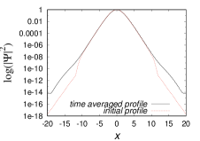
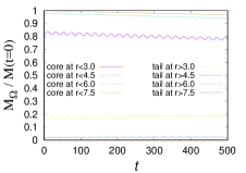
Figure 1: Evolution of a ground state equilibrium configuration on the domain $[-20,20]^{3}$ using isolated boundary conditions. (Top) Snapshots of the density $|\Psi|^{2}$ at various times that illustrates the core and the restless behavior of the density outside of the core. Also shown is the time average of the density profile from $t$=250 to $t$=500 together with the initial profile. (Bottom) Central density as function of time that shows the oscillations of the core and the mass calculated using different core radius $r_{c}=3,4.5,6.0$ and $7.0$.

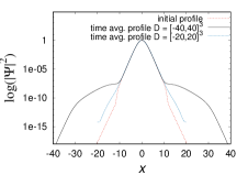
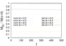
Figure 2: Evolution of a ground state equilibrium configuration on the domain $[-40,40]^{3}$ using isolated boundary conditions. (Top) Snapshots of the density $|\Psi|^{2}$ at various times that illustrates the core and the restless behavior of the density outside of the core. Also shown is the time average of the density profile from $t$=250 to $t$=500 together with the initial profile. (Bottom) Central density as function of time that shows the oscillations of the core and the mass calculated using different core radius $r_{c}=3,4.5,6.0$ and $7.0$.

We now evolve the same configuration using periodic boundary conditions. In this case the gravitational potential does not correspond to an isolated system and the boundary conditions at the faces of the cubic domain allow the potential to interact with itself, since the domain is a 3-Torus. The wave function is allowed to leak out from the gravitational potential well and redistribute across the domain, unlike the isolated case, where the sponge absorbs the density near the faces of the box. The evolution of the configuration is shown in Figure 3 for the small domain $[-20,20]^{3}$ and in Figure 4 for the big domain $[-40,40]^{3}$ that we describe together.

The first row of plots shows a set of snapshots of the density $|\Psi|^{2}$ starting from the initial configuration. Likewise in the isolated case above, a nearly stationary central core with the initial profile prevails, whereas the density outside the core has a very dynamical behavior and redistributes differently from the isolated case. The time average is also shown and indicates how the tail acquires a slow fall-off with distance that becomes nearly constant in the case of a big domain. The results of this distribution is only due to the periodicity of the domain. Notice that the nearly constant density of the tail is different for the small and big domains. If we consider the core radius $r_{c}=7.5$, we find that the mass of the tail redistributes with a factor of $\sim$8.5, which is the factor between the approximately constant tail densities in Figures 3 and 4.

The second row of results contains the central density as function of time that illustrates the oscillations of the core density, with a frequency that can be associated to the fundamental quasi normal modes, in this case for a soliton on top of a background density, unlike in vacuum Guzmán (2019). The simulation in the big domain develops a superposed mode that is not seen in the results in the small domain. It is also shown the conservation of mass of the core and tail using different values of the core radius. Notice that unlike the isolated domain, these quantities are better preserved during the evolution since there is no sponge where part of the density would sink.

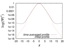
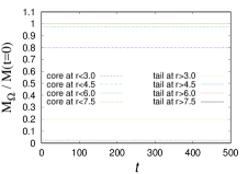
Figure 3: Evolution of a ground state equilibrium configuration on the domain $[-20,20]^{3}$ using periodic boundary conditions. (Top) Snapshots of the density $|\Psi|^{2}$ at various times that illustrates the core and the restless behavior of the density outside of the core. Also shown is the time average of the density profile from $t$=250 to $t$=500 together with the initial profile. (Bottom) On the left the central density as function of time that shows the oscillations of the core and on the right the mass of core and tail, with respect to their initial value using different core radius $r_{c}=3,4.5,6.0$ and $7.0$.

A summary of results is that the time-average core density profile is independent of the domain size, although it oscillates with modes that are excited differently for different domain size. The tail has a different profile, because the mass distributes in a bigger volume for the domain $[-40,40]^{3}$ than in the case $[-20,20]^{3}$.

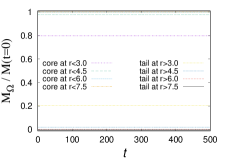
Figure 4: Evolution of a ground state equilibrium configuration on the domain $[-40,40]^{3}$ using periodic boundary conditions. (Top) Snapshots of the density $|\Psi|^{2}$ at various times that illustrates the core and the restless behavior of the density outside of the core. Also shown is the time average of the density profile from $t$=250 to $t$=500, together with the time average solution on the domain $[-20,20]^{3}$ and the initial density. (Bottom) On the left the central density as function of time that shows the oscillations of the core and on the right the mass of core and tail with respect to their initial time using various values of the core radius $r_{c}=3,4.5,6.0$ and $7.0$.

In order to investigate whether periodic boundary conditions trigger the extra oscillation mode seen in the solution with the big domain, we calculate the Fourier Transform of the central density as function of time from Figures 3 and 4 and two other simulations using spatial domains $[-30,30]^{3}$ and $[-50,50]^{3}$ to see the effects of domain size better. The results appear in Figure 5. The FT of the evolution using isolation conditions shows two main peaks at frequencies at 1 and at $\sim 1.768$, which coincide with the two first modes of oscillation when a ground state configuration is perturbed with a spherical perturbation Guzmán (2019).

When using periodic boundary conditions, the use of a bigger domain adds power to the second mode, which is reflected in the height of the second peak in the figure. Based on this observation, the mode superposed on the time-series of the central density of Figure 4 can be associated to the second mode of ground state equilibrium configurations, and is not a new oscillation mode, however excited by the reentrance of matter into the domain.

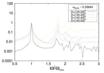
Figure 5: Fourier Transform of the central density as function of time, resulting from the evolution of a ground state equilibrium configuration. At the top the case of an isolated domain, where the two first modes resulting from a spherical perturbation with peaks at 1 and at $\sim 1.768$, as found in Guzmán (2019). At the bottom we show the result when using periodic boundary conditions with two peaks at frequencies 1 and $\sim 1.78$. There is a second peak with high power attributed to the distortion seen in Figure 4. This second peak gains power with the domain size, but it appears at the same location of the second mode of ground state equilibrium solutions as discussed in Guzmán (2019).

IV.2 Relaxation of a Near-Equilibrium Gaussian

A second problem is the dynamical relaxation of a spherically-symmetric object in near equilibrium, with a Gaussian density profile, as sometimes used to approximate the numerical ground-state equilibrium solution analytically. In this case, we adopt the initial conditions $\Psi({\bf x},0)=Ae^{-r^{2}/(2\sigma^{2})}$, $A=\sqrt{8}(\frac{K^{3}}{27\pi^{3}M})^{1/4}$ and $\sigma=\sqrt{\frac{3M}{4K}}$ with approximately the same mass $M$ and kinetic energy $K$ as that of the equilibrium configuration above. The evolution is carried out again in domains $[-20,20]^{3}$ and $[-40,40]^{3}$, covered with the same resolution as in the equilibrium configuration case.

The evolution of the fluctuation using isolation boundary conditions is illustrated with the results in Figures 6 and 7, that respectively correspond to the use of domains $[-20,20]^{3}$ and $[-40,40]^{3}$. In the two cases a core is formed that can be fit with the empirical formula (19), and coincides with the equilibrium density profile. The tail density falls rapidly towards the boundary where the sponge absorbs the density. The central density tends to stabilize, whereas the mass in the time window used decreases linearly but slowly, slower in the big domain, which illustrates the effects of the sponge, that is, the dynamical behavior of the tail region permanently pumps matter, even if in small quantities, toward the boundary, where it is absorbed.

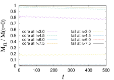
Figure 6: Evolution of a Gaussian in the domain $[-20,20]^{3}$ using isolated boundary conditions. (Top) Snapshots of the density $|\Psi|^{2}$ at various times that illustrates the core formation and the restless behavior of the density outside of the core. Also shown is the time average of the density profile from $t$=250 to $t$=500 together with the solitonic fitting profile. (Bottom) On the left the central density as function of time that shows the oscillations of the core and on the right the mass of core and tail with respect to their initial value using various values of the core radius $r_{c}=3,4.5,6.0$ and $7.0$.

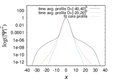
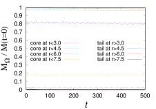
Figure 7: Evolution of a Gaussian in the domain $[-40,40]^{3}$ using isolated boundary conditions. (Top) Snapshots of the density $|\Psi|^{2}$ at various times that illustrates the core formation and the restless behavior of the density outside of the core. Also shown is the time average of the density profile from $t$=250 to $t$=500 together with the solitonic fitting profile. (Bottom) On the left the central density as function of time that shows the oscillations of the core and on the right the mass of core and tail with respect to their initial value using various values of the core radius $r_{c}=3,4.5,6.0$ and $7.0$.

The results are different when periodic boundary conditions are used. The results obtained for the relaxation of the Gaussian pulse are shown in Figures 8 and 9, corresponding to the use of domains $[-20,20]^{3}$ and $[-40,40]^{3}$. This time the initial conditions are not the soliton itself, but the soliton gets formed during the evolution with the profile (19). The density in the tail region is restless with an endless motion that in average distributes in a nearly constant profile, unlike the NFW decay found in structure formation halos Schive et al. (2014a); Mocz et al. (2017). We observe that the Gaussian pulse does not fragment, whereas the solitonic cores obtained from structure formation simulations result from the interference of multiple density fluctuations and are the superposition of many smaller fluctuations as shown later on in this paper. From these two simulations one can infer that the matter outside of the core distributes with a nearly constant profile, with a value that depends on the volume out of the core, which in turn depends on the domain size. A clear difference in comparison with the isolated case is that mass is not being lost during the evolution as expected from the topology of the domain.

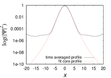
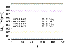
Figure 8: Evolution of a Gaussian in the domain $[-20,20]^{3}$ with periodic boundary conditions. (Top) Snapshots of the density $|\Psi|^{2}$ at various times that illustrates core and the restless behavior of the density outside of the core. Also shown is the time average of the density profile from $t$=250 to $t$=500 next to the initial configuration. (Bottom) On the left the central density as function of time that shows the oscillations of the core and on the right the of mass of core and tail and with respect to their initial time using various values of the core radius $r_{c}=3,4.5,6.0$ and $7.0$.

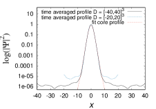
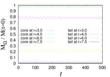
Figure 9: Evolution of a Gaussian in the domain $[-40,40]^{3}$ with periodic boundary conditions. (Top) Snapshots of the density $|\Psi|^{2}$ at various times that illustrates core and the restless behavior of the density outside of the core. Also shown is the time average of the density profile from $t$=250 to $t$=500 next to the initial configuration. (Bottom) On the left the central density as function of time that shows the oscillations of the core and on the right the of mass of core and tail and with respect to their initial time using various values of the core radius $r_{c}=3,4.5,6.0$ and $7.0$.

IV.3 Free-fall head-on merger

Another scenario that may be affected by the change of topology of the domain is the merger of two structures, as the gravitational potential repeats itself in copies outside of the domain along the three Cartesian directions. For this study, we focused on the head-on collision of two ground state equilibrium configurations in free-fall.

To illustrate this scenario, we conducted simulations in the domains $[-20,20]^{3}$ and $[-40,40]^{3}$ using the same space and time resolution as in the previous examples. We selected three cases with initial positions of the configurations at A) $(\pm 5,0,0)$, B) $(\pm 10,0,0)$ and C) $(\pm 15,0,0)$. It is expected that the domain outside of the box, which is plagued with a network of similar binary configurations, will have an effect on the collision dynamics. For comparison, we also simulated the merger using isolated boundary conditions.

The simulations results for Case A are presented in Figure 10. The left column displays the gravitational potential along the $x-$direction, while the right column shows the head-on momentum $\langle p_{x}\rangle$ integrated over the half-domains $x<0$ and $x>0$. In the first row, the results using isolation boundary conditions are presented, and the merger time is identified at $t\sim 14.9$, which is defined as the moment when the maximum head-on momentum is acquired. In the second and third rows, the results using periodic boundary conditions with domains $[-20,20]^{3}$ and $[-40,40]^{3}$ are shown, respectively. It can be observed that the merger time is affected by the periodic domain size; when using a small domain, the pull of the neighboring gravitational potentials retards the merger time. Furthermore, the magnitude of the momentum is also affected by the periodic domain.

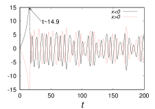
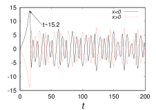
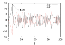
Figure 10: Case A. Head-on momentum $\langle p_{x}\rangle$ integrated in the semi-domains $x<0$ and $x>0$. At the top we show the results for the free-fall head-on merger using isolation boundary conditions. In second and third rows we show the momentum in the case of a periodic domain $[-20,20]^{3}$ and $[-40,40]^{3}$ respectively. The magnitude of the momentum is smaller when using a periodic domain, whereas the time of the maximum momentum is affected by the domain size.

Case B presents a different situation. It is a borderline case because the periodic boundary conditions imply the existence of a similar binary configuration on neighboring domains located at exactly the same distance, of 20 units of length along the $x-$axis. Binary configurations along the $y$ and $z$ axes will be separated by 40 length units from one another. This means that the binary configuration with periodic boundary conditions actually represents an infinite array of cores along the $x-$axis, equally spaced by 20 units of length and by 40 units along $y$ and $z$. The gravitational field is expected to be compensated along the $x-$direction in some way.

The results for Case B are shown in Figure 11. On the left, we present the gravitational potential along the $x-$direction, while on the right, we display $\langle p_{x}\rangle$ for the simulations with the isolated domain, periodic domain $[-20,20]^{3}$, and periodic domain $[-40,40]^{3}$, respectively. The first row corresponds to the head-on merger used as a control case that is not affected by the periodic domain.

The second row is the most noteworthy, as it takes a longer time for the cores to merge. This scenario requires further explanation since one might expect that the cores would never merge, given that they have infinite copies of themselves along the $x-$direction, and the gravitational effects along this direction would compensate and prevent the merger. However, the use of periodic boundary conditions introduces a subtlety, as seen in the left plots, where the gravitational potential is not zero at the center of the domain as it is at the boundary face. This effect has not been discussed in the literature on FDM simulations using periodic conditions, and it could have a significant influence on the results. It would be interesting to discuss and compare among codes and numerical implementations. Despite this asymmetry, the cores ultimately collide at the center of the domain after 115 time units.

The third row of results shows that with a bigger periodic domain, the collision time is more similar to that of the isolated case. This is because the potential wells of the cores of neighboring domains along the $x-$direction are further away from the binary system.

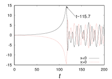
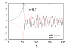
Figure 11: Case B. Form top to bottom results for the isolated domain $[-20,20]^{3}$, periodic domain $[-20,20]^{3}$ and periodic domain $[-40,40]^{3}$. At the left we show the gravitational potential at initial time along the $x-$axis, in order to illustrate its local minimums and behavior at the boundary. Particularly interesting is the second row, where the gravitational potentials of the cores are possibly expected to compensate each other along the $x-$direction. At the right we show $\langle p_{x}\rangle$ integrated in the semi-domains $x<0$ and $x>0$, as function of time.

Case C shows a more significant contribution of the boundary conditions. Instead of being pulled towards each other, the two solitons are pulled by their equivalent counterparts from the neighboring domains along the $x$-direction. The results are presented in Figure 12. It is worth noting that in the isolated scenario, the solitons collide frontally, whereas in the periodic domain, they collide from the “behind”, as evidenced by the linear momentum, which is positive for $x>0$ and negative for $x<0$. This indicates that initially they are moving apart from each other.

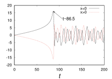
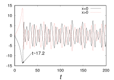
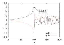
Figure 12: Case C. Form top to bottom results for the isolated domain $[-20,20]^{3}$, periodic domain $[-20,20]^{3}$ and periodic domain $[-40,40]^{3}$. At the left we show the gravitational potential at initial time along the $x-$axis. At the right we show $\langle p_{x}\rangle$ integrated in the semi-domains $x<0$ and $x>0$, as function of time.

IV.4 Merger in orbit

This is a case where the collision between two solitons has orbital angular momentum. We present an illustrative example for the initial conditions with the solitons centered at $(-10,10,0)$ and $(10,-10,0)$ and initial velocities $v_{x0}=0.1$ and $-0.1$ respectively. We evolve the system in the domain $D=[-40,40]^{3}$ using isolated boundary conditions, and domains $D=[-20,20]^{3}$ and $[-40,40]^{3}$ using periodic boundary conditions.

As observed in previous studies such as Schwabe et al. (2016); Guzmán et al. (2021), when the system is isolated, a significant portion of matter and angular momentum is radiated away. However, using a periodic domain allows for the re-entry of matter and angular momentum, which can then combine with the binary system. Figure 13 displays snapshots of isocontours of the density $|\Psi|^{2}$ at times $t=0,100,200,300,400,$ and $500$, from left to right, respectively.

Figure 13: Snapshots of the density level curves $|\Psi|^{2}$ at times $t=0,100,200,300,400$ and 500 for isolated boundary conditions in the domain $D=[-40,40]^{3}$ (top) , periodic boundary conditions in the domains $D=[-20,20]^{3}$ (middle) and $D=[-40,40]^{3}$ (bottom).

At the top of the Figure, we show the results using the isolated domain, indicating how the final configuration rotates and remains stable. In the middle row, we present snapshots of the evolution with periodic boundary conditions in the small domain. This can be ideally seen as an infinite network of equilibrium configurations, where the symmetry of the system and the domain size make the sum of the external forces near zero, leaving only the equilibrium configurations in uniform rectilinear motion, which is ideally eternal. This can be seen similarly to the boosted configuration presented in the Appendix. In the bottom row, we present snapshots of the density in the large periodic domain, which illustrates how the periodicity of the system enables the high kinetic energy matter expelled during the merger to re-enter and spread throughout the entire domain, ultimately leading to the formation of tail profiles. Notably, in both the isolated and periodic boundary condition cases for the domain $D=[-40,40]^{3}$, a single density distribution forms at the origin of coordinates, with its averaged profile along the $x$-axis shown in Figure 14. This profile is well-fitted by the core profile (19).

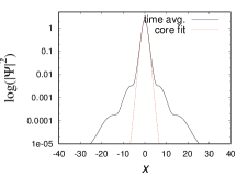
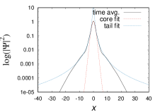
Figure 14: Time average of the density calculated over the interval $t\in[250,500]$ once the two equilibrium configurations have merged, simulated in the domain $[-40,40]^{3}$. On the left the case of isolated boundary conditions and on the right the case of periodic boundary conditions. Notice that the periodic domain allows the formation of a tail with polynomial profile.

Figure 15 shows the diagnostics for this system. The mass as a function of time indicates that in the periodic domain, the mass is conserved, while in the isolated case, there is a mass loss of approximately $28\%$ radiated out of the domain. Additionally, in the isolated domain, the angular momentum is carried out of the domain with the matter, while in the periodic domain, the reentrance is noticeable in the small domain. However, we do not observe any trend of $L_{z}$ in terms of the domain size.

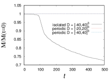
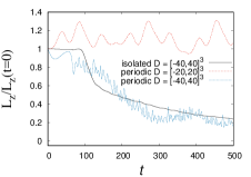
Figure 15: Evolution of a binary system with non-zero angular momentum, isolated boundary conditions in the domain $D=[-40,40]^{3}$ (solid black lines) and with periodic boundary conditions in the domains $D=[-20,20]^{3}$ (dotted red lines) and $D=[-40,40]^{3}$ (dashed blue lines). Evolution of the total mass $M$ and angular momentum $L_{z}$ as a functions of time.

IV.5 Merger of multiple cores

We investigate a final, more complex problem related to core formation. Drawing inspiration from previous studies Schwabe et al. (2016); Mocz et al. (2017); Li et al. (2021); Liu et al. (2023), we simulate the merger of $30$ equilibrium configurations with an ultralight bosonic mass of $m_{B}=10^{-22}eV/c^{2}$. These equilibrium configurations have random masses ranging from $2.6\times 10^{8}M_{\odot}$ to $26\times 10^{8}M_{\odot}$ and are initially positioned randomly within a cube of side length $30$ kpc, enabling comparison between the periodic and isolated boundary conditions. In the periodic domain case, we evolve the system in both a small cubic domain and a large cubic domain, with sides of 80 kpc and 100 kpc, respectively. We use the same random initial positions, configurations, and resolution in both cases, allowing us to isolate the effects of domain size on the dynamics of the system.

The results are summarized in Figure 16. On the left/right we show results obtained from simulations on the small/big domain. At the top we show some snapshots of the density projected on the $x-$axis, that show the dynamic behavior and interference patterns that change with time. In the mid row we show a snapshot of density in three-dimensions, at a time when the core is already formed. Finally, we calculate an average of the density in time and along various directions from the center of the core, in order to fit the core-tail structure that we show in the third row. The core is fitted using the function (19), using two methods. In the first method we fit the core with $r_{c}$ and $\rho_{0,core}$ as free parameters, the best fittings obtained with ($r_{c}\sim 0.228$kpc, $\rho_{0,core}\sim 2.42\times 10^{9}M_{\odot}/\textup{kpc}^{3}$) and ($r_{c}\sim 0.223$kpc, $\rho_{0,core}\sim 2.51\times 10^{9}M_{\odot}/\textup{kpc}^{3}$) in the small and big domains respectively, drawn with the blue line. The second method enforces the scaling relation $Mr_{c}\sim$constant to hold, which implies a constraint on the two free parameters; in this case the fitting parameters are ($r_{c}\sim 0.311$kpc, $\rho_{0,core}\sim 2.13\times 10^{9}M_{\odot}/\textup{kpc}^{3}$) and ($r_{c}\sim 0.309$kpc, $\rho_{0,core}\sim 2.19\times 10^{9}M_{\odot}/\textup{kpc}^{3}$) in the small and big domains respectively, whose profiles are represented with red lines. Finally, the tail is fitted with the NFW profile Navarro et al. (1997)

$$\rho_{tail}=\dfrac{\rho_{0,tail}}{\frac{r}{R_{s}}\left(1+\frac{r}{R_{s}}\right)^{2}}$$ (20)

with fitting parameters $\rho_{0,tail}\sim 4.6525\times 10^{5}M_{\odot}/\textup{kpc}^{3}$, $R_{s}\sim 7.473$ kpc for the small domain and $\rho_{0,tail}\sim 3.3\times 10^{5}M_{\odot}/\textup{kpc}^{3}$, $R_{s}\sim 8.67$ kpc for the big domain. The simulation lasts $\sim 12.7$Gyr, a time window within which none of the configurations has yet virialized, which explains why in the periodic domain case, the $Mr_{c}\sim constant$ constraint is not yet satisfied, e.g. as expected according to Liu et al. (2023).

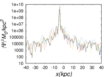
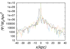
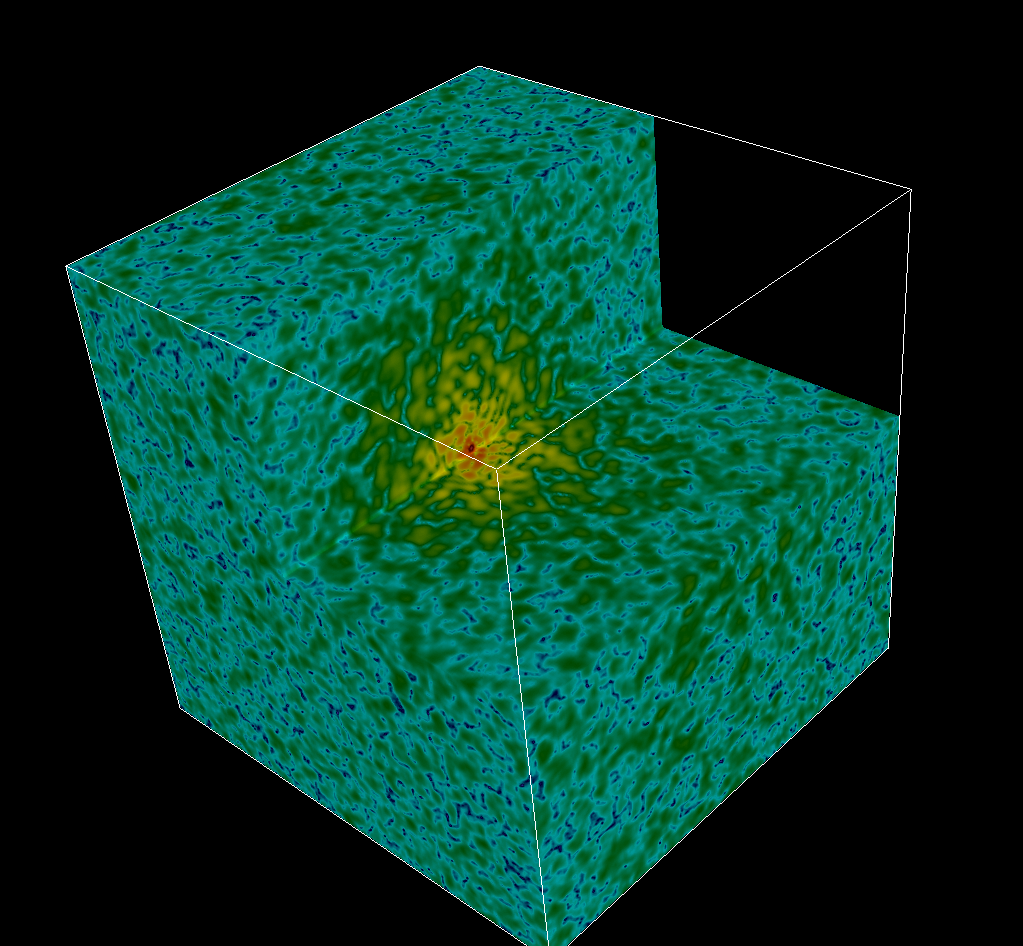
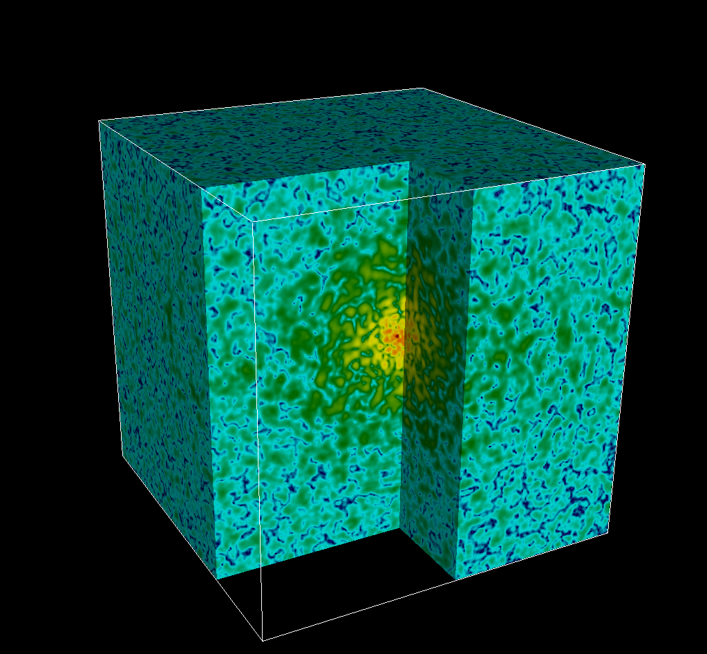
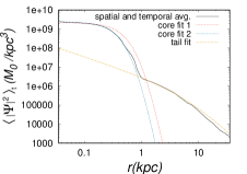
Figure 16: On the left/right we show results for the small/big domain. In the first row we show a few snapshots of the density along a line parallel to the $x-$axis that passes through the position of maximum density, which show how dynamic the system is. In the second row we show a volume view of the density illustrating the distribution of the bosonic cloud. In the third row we show the fit of density using formula (19) for the core and (20) for the NFW tail.

For comparison, we simulate this scenario using isolation conditions, where gravitational cooling is expected to drive the configuration toward an equilibrium solitonic profile in asymptotic time. We use the same numerical parameters as the periodic boundary simulation, with a domain of side 80 kpc and 30 solitons initially distributed in a box of side 30 kpc around the center of the domain. The results are summarized in Figure 17, which includes a few snapshots of the density along the $x$-axis, illustrating the concentration of density restricted by the presence of the sponge. Additionally, a volume view of the snapshots highlights the density concentration and the solitonic density profile.

The fitting parameters for the averaged core density profile in Eq. (19) using the first method with the two fitting parameters free are ($r_{c}=2.64$ kpc,$\rho_{0,core}=4.74\times 10^{5}{\rm M_{0}/kpc^{3}}$), whereas using the second method gives ($r_{c}=2.54$ kpc,$\rho_{0,core}=4.81\times 10^{5}{\rm M_{0}/kpc^{3}}$) when enforcing the condition $Mr_{c}\sim$constant. Notice that unlike the periodic domain, in this case the fitting profiles are very similar as illustrated with curves blue and red in the bottom of Figure 17. Finally, for completeness the parameters of a tail with the NFW profile are $\rho_{0,tail}\sim 1.74\times 10^{5}M_{\odot}/\textup{kpc}^{3}$, $R_{s}\sim 6.26$ kpc.

This simulation illustrates the dynamics of gravitational cooling in 3-D from initial conditions that are far from spherically symmetric. Previous work (see e.g. Guzmán and Ureña López (2006)) demonstrated that when initial conditions are spherically symmetric, gravitational cooling drives the configuration asymptotically towards the equilibrium ground-state solution of the solitonic core, with a density profile that drops steeply outside the core. Some nonsphericities were found to be expelled, as well, in simple axi-symmetric scenarios Bernal and Guzmán (2006b). As a result, it has been hypothesized that the solitonic core corresponding to the ground state is the attractor solution for a wider range of initial conditions, as long as gravitational cooling is permitted to occur and the system is allowed to evolve for a sufficient period to reach a state of relaxation.

Our simulation here represents an attempt to demonstrate this explicitly, in 3-D, from initial conditions that depart strongly from spherical symmetry, with control of gravitational cooling implemented via the isolating effects of the sponge boundary conditions. While the simulated time of order 12.7 Gyr is not long enough to allow the system to complete its relaxation to the asymptotic state of the ground state solution, it is clearly moving in that direction over time. By contrast, when the same initial configuration was simulated with periodic BC’s, with no sponge to absorb the mass and energy expelled by gravitational cooling, the density profile is fit by a solitonic core surrounded by a power-law envelope, or tail. Even though it is not fully relaxed by the final time-slice, the isolated case (i.e. with sponge) already shows a solitonic core surrounded by a profile that drops sharply toward large radius, much more steeply than in the case with periodic BC’s.

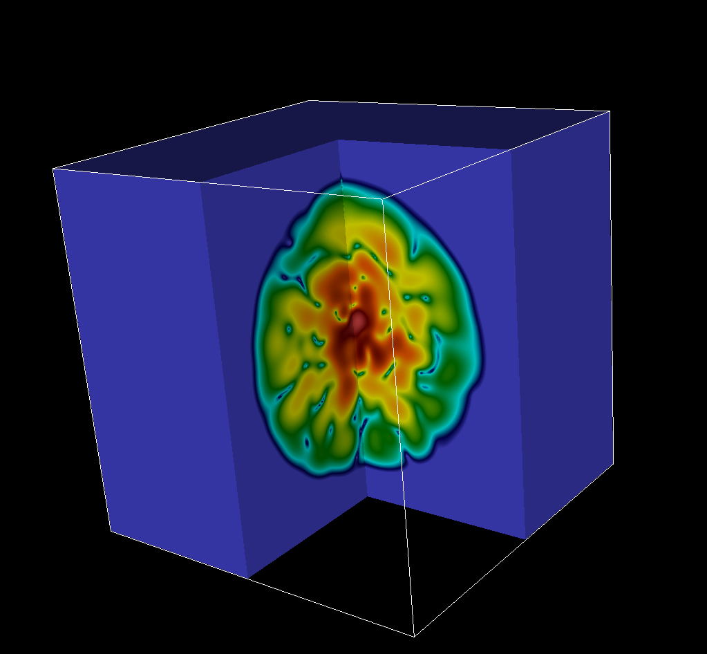
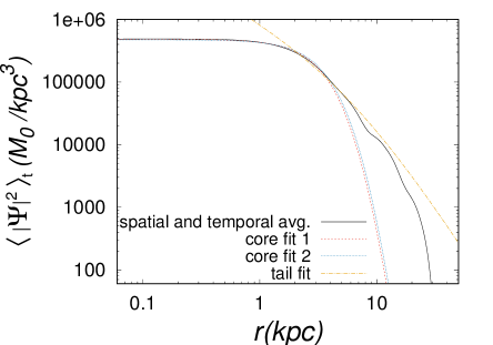
Figure 17: (Top) Snapshots of the density along the $x-$axis that illustrate how localized the density is. (Middle) Three dimensional view of the density that shows the concentration of matter inside the sponge region. (Bottom) Density profile and its comparison with fittings at core and tail regions; notice that the core fittings agree.

V Conclusions

This paper presents a comparison of the dynamics of FDM cores under different scenarios, utilizing both isolation and periodic boundary conditions.

Our analysis has yielded several observations for each scenario. In the simplest scenario, which involves the evolution of a ground-state equilibrium configuration of the SP system, we observed some distinct differences. Under periodic domain conditions, the density outside of the core, which decays exponentially, is redistributed into a nearly constant profile. Conversely, when using a sponge in the isolated domain, the density is forced to vanish near the boundary faces.

Our study demonstrates that the 3-D dynamical relaxation of a Gaussian density fluctuation near equilibrium results in the formation of a solitonic core, similar to the previously derived 1-D spherical symmetry ground-state equilibrium solution under isolated boundary conditions. However, notable differences emerge beyond the core, particularly in the tail zone. Under isolated domain conditions, the density in the tail decays exponentially with radius, while a nearly constant profile is observed when using a periodic domain.

Significant differences can be observed in the head-on merger of two configurations, particularly when solving the equations in a network of infinitely replicated configurations. In the most extreme case, a collision may occur through the backdoor of the domain.

During a merger of two orbiting configurations under periodic boundary conditions, it is possible that the merger may never occur. Additionally, the resulting configuration from a merger with angular momentum exhibits a tail with a density profile that is neither constant nor exponential, but rather polynomial. Notably, this configuration is connected and not fragmented, in contrast to those obtained from multi-mergers of cores and structure formation scenarios.

Lastly, we simulated the free-fall evolution of several cores to reproduce the formation of a structure with a core-tail density profile. Our simulations were conducted under both periodic boundary and isolation conditions, and we examined the effects of domain size on the density distribution. In the periodic domain, we observed that cores exhibited similar fitting parameters for two different box sizes, while the tail distribution varied. In contrast, under isolated conditions, we confirmed that there was virtually no tail.

The question of whether one BC choice is better or more realistic than the other is problem-specific. The isolating BC’s are perhaps most realistic when the object that forms is, itself, physically isolated from other objects and from infall of additional mass, so that its mass is no longer increasing by merger or infall – leaving it free to expel mass and energy to infinity, therefore, in the process of gravitational cooling, with plenty of time for it to reach the asymptotic equilibrium. The periodic BC’s, on the other hand, are most realistic when the opposite is occurring, that of objects that form by continuous mergers and mass assembly that is ongoing, so it prevents the free escape of mass and energy to infinity.

Our findings illustrate the quantitative impact of domain size on simulation results using periodic boundary conditions. These effects are worth evaluating in future studies of various astrophysical scenarios, as they can introduce uncertainties to numerical results.

Appendix A Tests of periodic boundary conditions

As a test of the correct implementation of periodic boundary conditions we evolve a boosted equilibrium configuration with initial speed $v_{x0}=1$, located initially at the center of the domain. When using a periodic domain the configuration should eternally travel crossing the domain periodically. There is no point of comparison between isolated and periodic domains for this scenario, nevertheless it turns out to be a good test for the implementation of periodic conditions.

In Figure 18 we show the density $|\Psi|^{2}$ along the $x-$axis at various times. The pulse travels from left to right, exits through the right end and reenters from the left as a result of the periodic domain. We also show the change of the total mass and energy with respect to its initial value, and see that both quantities are conserved with good precision, being the energy the most dissipated one, in less that $0.05\%$ during 50 crossing times.

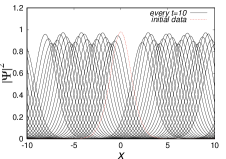
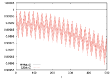
Figure 18: Evolution of an equilibrium configuration to which an initial velocity $v_{x0}=1$ is applied in the periodic domain $[-10,10]^{3}$. The left panel shows snapshots of the profile $|\Psi|^{2}$ along the $x$ axis every $t=10$ units of time. At the right side we show the mass and total energy as functions of time, normalized with respect to their initial value.

References

- Hu et al. (2000) W. Hu, R. Barkana, and A. Gruzinov, “Fuzzy Cold Dark Matter: The Wave Properties of Ultralight Particles,” Physical Review Letters 85, 1158–1161 (2000), astro-ph/0003365 .
- Matos and Ureña-López (2000) T. Matos and L. A. Ureña-López, “Quintessence and scalar dark matter in the Universe,” Classical and Quantum Gravity 17, L75–L81 (2000), astro-ph/0004332 .
- Sahni and Wang (2000) Varun Sahni and Limin Wang, “New cosmological model of quintessence and dark matter,” Phys. Rev. D 62, 103517 (2000).
- Hui et al. (2017) Lam Hui, Jeremiah P. Ostriker, Scott Tremaine, and Edward Witten, “Ultralight scalars as cosmological dark matter,” Phys. Rev. D 95, 043541 (2017).
- Hui (2021) Lam Hui, “Wave dark matter,” Annual Review of Astronomy and Astrophysics 59, 247–289 (2021).
- Niemeyer (2020) Jens C. Niemeyer, “Small-scale structure of fuzzy and axion-like dark matter,” Progress in Particle and Nuclear Physics 113, 103787 (2020).
- Ferreira (2021) Elisa G. M. Ferreira, “Ultra-light dark matter,” The Astronomy and Astrophysics Review 29, 7 (2021), arXiv:2005.03254 [astro-ph.CO] .
- Lee (2018) Jae-Weon Lee, “Brief History of Ultra-light Scalar Dark Matter Models,” EPJ Web Conf. 168, 06005 (2018), arXiv:1704.05057 [astro-ph.CO] .
- Suárez et al. (2014) Abril Suárez, Victor H. Robles, and Tonatiuh Matos, “A Review on the Scalar Field/Bose-Einstein Condensate Dark Matter Model,” Astrophys. Space Sci. Proc. 38, 107–142 (2014), arXiv:1302.0903 [astro-ph.CO] .
- Ruffini and Bonazzola (1969) R. Ruffini and S. Bonazzola, “Systems of self-gravitating particles in general relativity and the concept of an equation of state,” Phys. Rev. 187, 1767–1783 (1969).
- Guzmán and Ureña López (2004) F. S. Guzmán and L. A. Ureña López, “Evolution of the schrödinger-newton system for a self-gravitating scalar field,” Phys. Rev. D 69, 124033 (2004).
- Bernal and Guzmán (2006a) Argelia Bernal and F. S. Guzmán, “Scalar field dark matter: Head-on interaction between two structures,” Physical Review D 74 (2006a), 10.1103/physrevd.74.103002.
- Schwabe et al. (2016) Bodo Schwabe, Jens C. Niemeyer, and Jan F. Engels, “Simulations of solitonic core mergers in ultralight axion dark matter cosmologies,” Phys. Rev. D 94, 043513 (2016), arXiv:1606.05151 [astro-ph.CO] .
- Dawoodbhoy et al. (2021) Taha Dawoodbhoy, Paul R Shapiro, and Tanja Rindler-Daller, “Core-envelope haloes in scalar field dark matter with repulsive self-interaction: fluid dynamics beyond the de broglie wavelength,” Monthly Notices of the Royal Astronomical Society 506, 2418 – 2444 (2021).
- Du et al. (2018) Xiaolong Du, Bodo Schwabe, Jens C. Niemeyer, and David Bürger, “Tidal disruption of fuzzy dark matter subhalo cores,” Phys. Rev. D 97, 063507 (2018).
- Schive et al. (2014a) Hsi-Yu Schive, Tzihong Chiueh, and Tom Broadhurst, “Cosmic Structure as the Quantum Interference of a Coherent Dark Wave,” Nature Phys. 10, 496–499 (2014a), arXiv:1406.6586 [astro-ph.GA] .
- Mocz et al. (2017) Philip Mocz, Mark Vogelsberger, Victor H. Robles, Jesus Zavala, Michael Boylan-Kolchin, Anastasia Fialkov, and Lars Hernquist, “Galaxy formation with BECDM I. Turbulence and relaxation of idealized haloes,” Mon. Not. Roy. Astron. Soc. 471, 4559–4570 (2017), arXiv:1705.05845 [astro-ph.CO] .
- Mocz et al. (2019) Philip Mocz, Anastasia Fialkov, Mark Vogelsberger, Fernando Becerra, Mustafa A. Amin, Sownak Bose, Michael Boylan-Kolchin, Pierre-Henri Chavanis, Lars Hernquist, Lachlan Lancaster, and et al., “First star-forming structures in fuzzy cosmic filaments,” Phys. Rev. Lett. 123 (2019).
- Mocz et al. (2020) Philip Mocz, Anastasia Fialkov, Mark Vogelsberger, Fernando Becerra, Xuejian Shen, Victor H Robles, Mustafa A Amin, Jesus Zavala, Michael Boylan-Kolchin, Sownak Bose, Federico Marinacci, Pierre-Henri Chavanis, Lachlan Lancaster, and Lars Hernquist, “Galaxy formation with BECDM II. Cosmic filaments and first galaxies,” Mon. Not. R. Astron. Soc. 494, 2027–2044 (2020).
- Schwabe and Niemeyer (2022) Bodo Schwabe and Jens C. Niemeyer, “Deep zoom-in simulation of a fuzzy dark matter galactic halo,” Phys. Rev. Lett. 128, 181301 (2022).
- Seidel and Suen (1994) Edward Seidel and Wai-Mo Suen, “Formation of solitonic stars through gravitational cooling,” Phys. Rev. Lett. 72, 2516–2519 (1994).
- Guzmán and Ureña López (2006) F. S. Guzmán and L. Arturo Ureña López, “Gravitational cooling of self-gravitating bose condensates,” The Astrophysical Journal 645, 814 – 819 (2006).
- Navarro et al. (1997) Julio F. Navarro, Carlos S. Frenk, and Simon D. M. White, “A Universal Density Profile from Hierarchical Clustering,” Astrophys. J. 490, 493–508 (1997), arXiv:astro-ph/9611107 [astro-ph] .
- Marsh (2016) David J. E. Marsh, “Axion cosmology,” Physics Reports 643, 1–79 (2016), arXiv:1510.07633 [astro-ph.CO] .
- Jetzer (1992) Phillippe Jetzer, “Boson stars,” Physics Reports 220, 163–227 (1992).
- Membrado et al. (1989) M. Membrado, A. F. Pacheco, and J. Sañudo, “Hartree solutions for the self-Yukawian boson sphere,” Phys. Rev. A 39, 4207–4211 (1989).
- Schive et al. (2014b) Hsi-Yu Schive, Ming-Hsuan Liao, Tak-Pong Woo, Shing-Kwong Wong, Tzihong Chiueh, Tom Broadhurst, and W. Y. Pauchy Hwang, “Understanding the Core-Halo Relation of Quantum Wave Dark Matter from 3D Simulations,” Phys. Rev. Lett. 113, 261302 (2014b), arXiv:1407.7762 [astro-ph.GA] .
- Rindler-Daller and Shapiro (2014) Tanja Rindler-Daller and Paul R. Shapiro, “Complex Scalar Field Dark Matter on Galactic Scales,” Modern Physics Letters A 29, 1430002 (2014), arXiv:1312.1734 [astro-ph.CO] .
- Dawoodbhoy et al. (2021) Taha Dawoodbhoy, Paul R. Shapiro, and Tanja Rindler-Daller, “Core-envelope haloes in scalar field dark matter with repulsive self-interaction: fluid dynamics beyond the de Broglie wavelength,” Monthly Notices of the Royal Astronomical Society 506, 2418–2444 (2021), arXiv:2104.07043 [astro-ph.CO] .
- Shapiro et al. (2022) Paul R. Shapiro, Taha Dawoodbhoy, and Tanja Rindler-Daller, “Cosmological structure formation in scalar field dark matter with repulsive self-interaction: the incredible shrinking Jeans mass,” Monthly Notices of the Royal Astronomical Society 509, 145–173 (2022), arXiv:2106.13244 [astro-ph.CO] .
- Widrow and Kaiser (1993) Lawrence M. Widrow and Nick Kaiser, “Using the Schroedinger Equation to Simulate Collisionless Matter,” The Astrophysical journal Letters 416, L71 (1993).
- Mocz et al. (2018) Philip Mocz, Lachlan Lancaster, Anastasia Fialkov, Fernando Becerra, and Pierre-Henri Chavanis, “Schrödinger-Poisson-Vlasov-Poisson correspondence,” Phys. Rev. D 97, 083519 (2018), arXiv:1801.03507 [astro-ph.CO] .
- Madelung (1927) E. Madelung, “Quantentheorie in hydrodynamischer Form,” Zeitschrift fur Physik 40, 322–326 (1927).
- Bohm (1952a) David Bohm, “A suggested interpretation of the quantum theory in terms of ”hidden” variables. i,” Phys. Rev. 85, 166–179 (1952a).
- Bohm (1952b) David Bohm, “A suggested interpretation of the quantum theory in terms of ”hidden” variables. ii,” Phys. Rev. 85, 180–193 (1952b).
- Alvarez-Ríos and Guzmán (2022) Iván Alvarez-Ríos and Francisco S. Guzmán, “Construction and Evolution of Equilibrium Configurations of the Schrödinger–Poisson System in the Madelung Frame,” Universe 8, 432 (2022), arXiv:2210.15608 [gr-qc] .
- Takabayasi (1954) T. Takabayasi, “The Formulation of Quantum Mechanics in terms of Ensemble in Phase Space,” Progress of Theoretical Physics 11, 341–373 (1954).
- Wigner (1932) E. Wigner, “On the quantum correction for thermodynamic equilibrium,” Phys. Rev. 40, 749–759 (1932).
- Skodje et al. (1989) Rex T. Skodje, Henry W. Rohrs, and James VanBuskirk, “Flux analysis, the correspondence principle, and the structure of quantum phase space,” Phys. Rev. A 40, 2894–2916 (1989).
- HUSIMI (1940) K. HUSIMI, “Some formal properties of the density matrix,” Proceedings of the Physico-Mathematical Society of Japan. 3rd Series 22, 264–314 (1940).
- Ahn and Shapiro (2005) Kyungjin Ahn and Paul R. Shapiro, “Formation and evolution of self-interacting dark matter haloes,” Monthly Notices of the Royal Astronomical Society 363, 1092–1110 (2005), arXiv:astro-ph/0412169 [astro-ph] .
- Alvarez et al. (2003) M. A. Alvarez, K. Ahn, and P. R. Shapiro, “Density Profiles of Dark Halos from their Mass Accretion Histories,” in Revista Mexicana de Astronomia y Astrofisica Conference Series, Revista Mexicana de Astronomia y Astrofisica Conference Series, Vol. 18, edited by M. Reyes-Ruiz and E. Vázquez-Semadeni (2003) pp. 4–7, arXiv:astro-ph/0302336 [astro-ph] .
- Shapiro et al. (2004) Paul R. Shapiro, Ilian T. Iliev, Hugo Martel, Kyungjin Ahn, and Marcelo A. Alvarez, “The Equilibrium Structure of CDM Halos,” arXiv e-prints , astro-ph/0409173 (2004), arXiv:astro-ph/0409173 [astro-ph] .
- Shapiro et al. (2006) P. R. Shapiro, K. Ahn, M. Alvarez, I. T. Iliev, and H. Martel, “Understanding the Equilibrium Structure of CDM Halos,” in EAS Publications Series, EAS Publications Series, Vol. 20, edited by Gary A. Mamon, Francoise Combes, Cedric Deffayet, and Bernard Fort (2006) pp. 5–10, arXiv:astro-ph/0510146 [astro-ph] .
- Chavanis (2022) Pierre-Henri Chavanis, “A heuristic wave equation parameterizing BEC dark matter halos with a quantum core and an isothermal atmospher,” The European Physical Journal B 95, 48 (2022).
- Guzmán et al. (2014) F. S. Guzmán, F. D. Lora-Clavijo, J. J. González-Avilés, and F. J. Rivera-Paleo, “Rotation curves of rotating galactic bose-einstein condensate dark matter halos,” Phys. Rev. D 89, 063507 (2014).
- Alvarez-Rios and Guzman (2022) I. Alvarez-Rios and F. S. Guzman, “Exploration of simple scenarios involving fuzzy dark matter cores and gas at local scales,” (2022), arXiv:2207.00062 .
- Guzmán (2019) F. S. Guzmán, “Oscillation modes of ultralight bec dark matter cores,” Physical Review D 99 (2019), 10.1103/physrevd.99.083513.
- Guzmán et al. (2021) F. S. Guzmán, I. Alvarez-Ríos, and J. A. González, “Merger of galactic cores made of ultralight bosonic dark matter,” Rev. Mex. Fis. 67, 75–83 (2021).
- Li et al. (2021) Xinyu Li, Lam Hui, and Tomer D. Yavetz, “Oscillations and random walk of the soliton core in a fuzzy dark matter halo,” Physical Review D 103 (2021), 10.1103/physrevd.103.023508.
- Liu et al. (2023) I. Kang Liu, Nick P. Proukakis, and Gerasimos Rigopoulos, “Coherent and incoherent structures in fuzzy dark matter halos,” Monthly Notices of the Royal Astronomical Society (2023), 10.1093/mnras/stad591, arXiv:2211.02565 [astro-ph.CO] .
- Bernal and Guzmán (2006b) Argelia Bernal and F. S. Guzmán, “Scalar field dark matter: Nonspherical collapse and late-time behavior,” Physical Review D 74 (2006b), 10.1103/physrevd.74.063504.