upstreamFoam: an OpenFOAM-based solver for heterogeneous porous media at different scales

Abstract

A new OpenFOAM application to simulate multiphase flows in porous media is formulated and tested. The proposed solver combines the Eulerian multi-fluid formulation for a system of phase fractions with Darcy’s law for flows through porous media. It is based on the multiphaseEulerFoam and includes models for reservoir simulation of the porousMultiphaseFoam, taking advantage of the most recent technologies developed for these well-established solvers. With such an innovative combination, we are able to simulate a system of any number of compressible phase fractions in reservoirs that rely on specialized models for relative permeability, capillary pressure, and time step selection. We successfully validate the solver for classical problems with analytical, semi-analytical, and reference solutions. A wide range of flows in porous media has been studied, demonstrating the potential of the solver to approximate complex multiphase problems.

[inst1]organization=Wikki Brasil LTDA,addressline=Rua Paulo Emídio Barbosa, 485, sala 301, Parque Tecnológico da UFRJ, city=Rio de Janeiro, postcode=21941-907, state=RJ, country=Brazil

[inst2]organization=Petrobras Research Center (CENPES),addressline=Av. Horácio Macedo 950, Cidade Universitária, Ilha do Fundão, city=Rio de Janeiro, postcode=21941-598, state=RJ, country=Brazil

1 Introduction

Multiphase flows describe several problems with applications in various fields. The Computational Fluid Dynamics (CFD) approaches have been extensively used for multiphase flows modeling and simulation [1]. Implementation of methodologies for solving CFD problems within open-source simulators is gaining popularity in industrial and academic research groups. The OpenFOAM library is an example, which is based on the Finite Volume Method (FVM) and covers a variety of cases [2, 3].

A well-known procedure for solving CFD problems is the Eulerian multi-fluid model [4, 5], which describes a system of phase fractions represented by averaged conservation equations [6, 7]. In this context, work [8] should be highlighted, where a conservative and bounded formulation based on a volumetric average for the momentum exchange terms has been presented.

There are different solution procedures for multiphase flow problems available in OpenFOAM. In the framework of Eulerian fluid models, the solver twoPhaseEulerFoam has been proposed, initially to simulate incompressible two-phase flows [9]. In [10], the effects of particle-particle interaction have been included by coupling the population balance equation with the twoPhaseEulerFoam. Then, the solver was extended to $n+1$ phases, considering a continuous phase and $n$ dispersed phases [11, 12]. Another solver, the multiphaseEulerFoam, has been developed to combine the Eulerian multi-fluid solution framework with the Volume of Fluid (VOF) method for interface capturing on selected phase pairs [13]. The proposed hybrid multiphase CFD solver employs the interface compression methodology of [14]. The multiphaseEulerFoam considers a system of any number of compressible fluid phases with a common pressure, but with other separate properties. This approach allows for solving complex flows with multiple species, heat and mass transfer, being widely used [15].

A wide range of multiphase flow applications occurs within porous media [16]. The subsurface flows in oil reservoirs are relevant examples of such topics [17]. In the last years, several computational models for simulating multiphase flows in porous media have been introduced [18]. An increase in the development of open-source simulators for this class of problems is also noticeable.

Regarding the OpenFOAM approach, a remarkable toolbox to simulate incompressible two-phase flows in porous media, called porousMultiphaseFoam, has been introduced in [19]. This development includes a formulation for the phase saturations, relative permeability and capillary models, and special boundary conditions. Extensions of the porousMultiphaseFoam include an approach for adaptive mesh refinement [20] and a generalization for the black oil model [21]. In [22], recent developments have been presented, such as improved numerical techniques for hydrogeological flows modeling and the transport problem of a mixture with $n$ components. The porousMultiphaseFoam has also been used as the basis for the development of a hybrid approach to simulate two-phase flows in systems containing solid-free regions and porous matrices [23], besides that a two-phase flow procedure coupled with geomechanics and Embedding Discrete Fracture Model (EDFM) [24].

In this paper, we develop a solver for multiphase flows in porous media combining the Eulerian multi-fluid formulation for a system of phase fractions with the Darcy’s law for flows through porous media [25]. The proposed approach, implemented in OpenFOAM, is based on the multiphaseEulerFoam and includes models for reservoir simulation of the porousMultiphaseFoam, in addition to introducing new features and formulations. We leverage the capability of the multiphaseEulerFoam to simulate a system of any number of phase fractions at a common pressure, with the possibility of adding phase compressibility, multiple species, and mass transfer. Moreover, we take advantage of the treatment for essential aspects of reservoir simulation, such as the relative permeability, capillarity models, and specific boundary conditions provided by porousMultiphaseFoam. With the new toolbox, called upstreamFoam, it is possible to handle complex simulations of compressible multiphase flows in porous media. A distinguish property of the method presented here is the formulation of the solid as a stationary phase, which allows for the use of different minerals or different types of solid.

The multiphase porous media model requires the solution of a system of coupled nonlinear partial differential equations, approximated by the IMplicit Pressure Explicit Saturation (IMPES) scheme [26]. We show the segregated algorithm used, the conservation equations, and the relationship between the formulation based on phase fractions and other common approaches based on saturations. Furthermore, we highlight details about the reservoir characterization and the treatments given for the heterogeneous permeability field and time-step choice.

The paper is divided into sections as follows. In section 2, the mathematical model is presented, followed by the numerical formulation in section 3, numerical results in section 4, and conclusions in section 5.

2 Mathematical Model

The mathematical model for flows in porous media is given by volume averaged equations, where each volume contains both solid and void space. The void space, in turn, can contain multiple fluids. In the next subsections, porous media definitions and conservation principles that describe flows in porous media are presented.

2.1 Porous media definitions

The void space of a porous medium is represented by the porosity filed

$$\alpha_{v}=\frac{V_{v}}{V},$$ (1)

where $V_{v}$ is the volume occupied by the void space and $V$ is the volume of the respective cell, that is, the porosity is the void fraction and satisfies $0\leq\alpha_{v}\leq 1$, where $\alpha_{v}=0$ indicates an impermeable medium and $\alpha_{v}=1$ a totally free region. We consider a system of phase fractions $\alpha_{i}$, in which the index $i$ represents one phase of the flow, such that for each cell

$$\alpha_{i}=\left\{\begin{array}[]{ll}0,&\mbox{cell does not contain phase }i,\\ ]0,1[\,,&\mbox{cell contains phase }i\mbox{ and other phases},\\ 1,&\mbox{cell is completely filled with phase }i.\end{array}\right.$$ (2)

Phase fractions satisfy the following relationship

$$\sum_{i=1}^{N_{s}}\alpha_{i}+\sum_{i=1}^{N_{m}}\alpha_{i}=1,$$ (3)

where $N_{s}$ is the number of stationary phases and $N_{m}$ is the number of moving phases of the system. The total number of phases is denoted by $N=N_{s}+N_{m}$. In terms of the void fraction we have

$$\alpha_{v}=1-\sum_{i=1}^{N_{s}}\alpha_{i}.$$ (4)

It is important to notice that the solid is treated as a stationary phase, allowing to define different minerals or different types of solid as different stationary phases.

Formulations based on saturations are more common than the phase fractions approach, however, the relationship between both consists in the fact that the saturation of a phase can be written as

$$S_{i}=\frac{\alpha_{i}}{\alpha_{v}}.$$ (5)

Another advantage of the formulation based on phase fractions is the possibility of considering residual saturations as stationary phases.

2.2 Conservation equations

In the context of porous media flows, the momentum balance equation of each phase fraction reduces to the Darcy’s law [25]:

$$\alpha_{i}\mathbf{u}_{i}=-\frac{k_{r,i}}{\mu_{i}}\,\mathbf{K}\cdot\left(\nabla p_{i}-\rho_{i}\mathbf{g}\right),$$ (6)

in which, $\mathbf{u}_{i}$ is the velocity of the phase $i$, $k_{r,i}$ is the phase relative permeability, $\mu_{i}$ is the dynamic viscosity of the phase, $\mathbf{K}$ is the absolute permeability tensor, $p_{i}$ is the pressure of the phase, $\rho_{i}$ is the density of phase, and $\mathbf{g}$ is the gravity acceleration.

The pressure gradient $\nabla p_{i}$ can be replaced using a modified pressure $p_{i}^{*}$ as follows:

$$\nabla p_{i}=\nabla p_{i}^{*}+\nabla\left(\rho_{m}(\mathbf{g}\cdot\mathbf{h})\right),$$ (7)

where the term $\rho_{m}(\mathbf{g}\cdot\mathbf{h})$ represents a pseudo-hydrostatic pressure, $\mathbf{h}$ is the height of the fluid particle, and $\rho_{m}$ is the fluid mixture density, defined as

$$\rho_{m}=\sum_{i=1}^{N_{m}}\alpha_{i}\rho_{i}.$$ (8)

Substituting Eq. (7) in Eq. (6) and rearranging, yields:

$$\alpha_{i}\mathbf{u}_{i}=-\frac{k_{r,i}}{\mu_{i}}\,\mathbf{K}\cdot\Big{(}\nabla p^{*}_{i}-(\rho_{i}-\rho_{m})\mathbf{g}+(\mathbf{g}\cdot\mathbf{h})\nabla\rho_{m}\Big{)}.$$ (9)

The mass balance equation for each phase reads:

$$\frac{\partial\alpha_{i}\rho_{i}}{\partial t}+\nabla\cdot(\alpha_{i}\rho_{i}\mathbf{u}_{i})=q_{i},$$ (10)

where $q_{i}$ is the source term related to the phase $i$. Equation (10) can be expanded and rewritten as

$$\frac{\partial\alpha_{i}}{\partial t}+\nabla\cdot\left(\alpha_{i}\mathbf{u}_{i}\right)=\frac{q_{i}}{\rho_{i}}-\frac{\alpha_{i}}{\rho_{i}}\frac{D_{i}\rho_{i}}{Dt},$$ (11)

where the material derivative of $\rho$, which accounts for the compressibility effects, is given by

$$\frac{D\rho_{i}}{Dt}=\frac{\partial\rho_{i}}{\partial t}+\mathbf{u}_{i}\cdot\nabla\rho_{i}.$$ (12)

Another important concept is the mixture velocity $\mathbf{u}_{m}$ which, for $N$ phases, is given by

$$\mathbf{u}_{m}=\sum_{i=1}^{N}\alpha_{i}\mathbf{u}_{i}.$$ (13)

Moreover, the relative velocity between two phases $i$ and $j$ is defined as

$$\mathbf{u}_{r,ij}=\mathbf{u}_{i}-\mathbf{u}_{j}.$$ (14)

Then, summing the mass conservation equations of all phases and using the relation of Eq. (3), the total mass conservation can be written as

$$\nabla\cdot\mathbf{u}_{m}=\sum_{i=1}^{N}\frac{q_{i}}{\rho_{i}}-\sum_{i=1}^{N}\frac{\alpha_{i}}{\rho_{i}}\frac{D_{i}\rho_{i}}{Dt}.$$ (15)

Considering the concepts of mixture velocity and relative velocity, it is possible to express the general transport equation for each phase fraction $\alpha_{i}$ as

$$\frac{\partial\alpha_{i}}{\partial t}+\nabla\cdot\left(\alpha_{i}\mathbf{u}_{m}\right)+\sum_{\begin{subarray}{c}j=1\\ j\neq i\end{subarray}}^{N}(\nabla\cdot\left.\left(\alpha_{i}\alpha_{j}\mathbf{u}_{r,ij}\right)\right) =\frac{q_{i}}{\rho_{i}}+\alpha_{i}\nabla\cdot\mathbf{u}_{m}$$ (16)

$$-\frac{\alpha_{i}}{\rho_{i}}\frac{D_{i}\rho_{i}}{Dt}+\alpha_{i}\sum_{j=1}^{N}\frac{\alpha_{j}}{\rho_{j}}\frac{D_{j}\rho_{j}}{Dt}.$$

Equation (16) was obtained following the conservative formulation for phase continuity equations developed in [8, 11, 27].

2.2.1 Capillary effects

The discontinuity between two moving phases of a multiphase flow on porous media generates an additional relationship between pressure fields denominated as capillary pressure $p_{c}$, given by:

$$p_{c,ki}=p^{*}_{k}-p^{*}_{i},$$ (17)

in which $k$ is a reference phase and $i$ is any other phase of the system.

Using the definition of capillary pressure in Eq. (17) to replace the pressure of phase $p_{i}^{*}$ in Eq. (9), one can write:

$$\alpha_{i}\mathbf{u}_{i}=-\frac{k_{r,i}}{\mu_{i}}\mathbf{K}\cdot\Big{(}\nabla p^{*}_{k}-\nabla p_{c,ki}-(\rho_{i}-\rho_{m})\mathbf{g}+(\mathbf{g}\cdot\mathbf{h})\nabla\rho_{m}\Big{)}$$ (18)

Therefore, the pressure of any phase $i$ is defined as a function of the pressure of the reference phase $k$ and the capillary pressure of the pair $ki$. Note that for the reference phase, the capillary pressure satisfies $p_{c,kk}=0$, and hence Eq. (9) does not change.

2.3 Summary of the formulation

In summary, the mathematical model for compressible multiphase flows in porous media, explained above, consists of a set of partial differential equations, namely the momentum balance equation for each phase fraction, Eq. (18), a total mass balance equation, Eq. (15), and the transport equation of each phase fraction, Eq. (16):

$$\alpha_{i}\mathbf{u}_{i}=-\frac{k_{r,i}}{\mu_{i}}\mathbf{K}\cdot\Big{(}\nabla p^{*}_{k}-\nabla p_{c,ki}-(\rho_{i}-\rho_{m})\mathbf{g}+(\mathbf{g}\cdot\mathbf{h})\nabla\rho_{m}\Big{)}$$ (19)

$$\nabla\cdot\mathbf{u}_{m}=\sum_{i=1}^{N}\frac{q_{i}}{\rho_{i}}-\sum_{i=1}^{N}\frac{\alpha_{i}}{\rho_{i}}\frac{D_{i}\rho_{i}}{Dt}$$

$$\frac{\partial\alpha_{i}}{\partial t}+\nabla\cdot\left(\alpha_{i}\mathbf{u}_{m}\right)+\sum_{\begin{subarray}{c}j=1\\ j\neq i\end{subarray}}^{N}(\nabla\cdot\left.\left(\alpha_{i}\alpha_{j}\mathbf{u}_{r,ij}\right)\right)=\frac{q_{i}}{\rho_{i}}+\alpha_{i}\nabla\cdot\mathbf{u}_{m}$$

$$\hskip 204.85974pt-\frac{\alpha_{i}}{\rho_{i}}\frac{D_{i}\rho_{i}}{Dt}+\alpha_{i}\sum_{j=1}^{N}\frac{\alpha_{j}}{\rho_{j}}\frac{D_{j}\rho_{j}}{Dt}.$$

In the next section, we detail the numerical treatment for approximating and solution of the model system of equations Eq. (19).

3 Numerical Formulation

In this section, we describe the algorithm used to solve the nonlinear system for multiphase flows in porous media along with some models considered and their particularities.

3.1 Solution approach

Te segregated IMPES scheme [26] is considered, where the global mass conservation, expressed by a pressure equation, is implicitly solved, while the phase fractions are explicitly solved.

In order to write the system for pressure and phase fractions, the total mass conservation Eq. (15) is coupled with the momentum balance Eq. (18), resulting in the following expression:

$$\nabla\cdot\left[\ \sum_{i=1}^{N}\left(\frac{k_{r,i}}{\mu_{i}}\,\mathbf{K}\cdot\Big{(}\nabla p_{k}^{*}-\nabla p_{c,ki}-\left(\rho_{i}-\rho_{m}\right)\mathbf{g}+(\mathbf{g}\cdot\mathbf{h})\nabla\rho_{m}\Big{)}\right)\right]=-\sum_{i=1}^{N}\frac{q_{i}}{\rho_{i}}$$ (20)

$$+\sum_{i=1}^{N}\frac{\alpha_{i}}{\rho_{i}}\frac{D_{i}\rho_{i}}{Dt}.$$

Note that only one pressure equation is obtained for the system instead of a pressure equation for each phase. The total flux $\phi$ resulting from the pressure equation can be decomposed as

$$\phi=\phi_{p}+\phi_{p_{c}}+\phi_{g},$$ (21)

where $\phi_{p}$, $\phi_{p_{c}}$, and $\phi_{g}$ represent the flux contributions generated, respectively, by the pressure gradient, capillary pressure and gravity driving forces. The reformulated system is in agreement with the basic framework of OpenFOAM for velocity and pressure coupling. To approximate the pressure-velocity coupling, a solver based on Pressure IMplicit with splitting of operator for Pressure-Linked Equations (PIMPLE) available in OpenFOAM [28] is used.

As a classic finite volume-based numerical scheme, our solver considers the variables calculated in the cell center and interpolated to the faces if necessary. The upstreamFoam has an additional option of constructing term by term of the momentum equation interpolated on the faces of the control volumes. This option increases the numerical stability and accuracy of the balance of forces. To interpolate the different variables distinct numerical schemes are used, for example, linear interpolation, first-order upwind scheme, and harmonic average.

3.1.1 Algorithm

The numerical scheme considers the following sequence at each time step:

1. The phases fractions are solved explicitly using the last known information;

2. Relative permeability, density, viscosity, and other properties are updated using the new value of the phases fractions;

3. The pressure-velocity coupling is solved.

3.1.2 Time-step limitations

The phases fractions are solved explicitly using the Multidimensional Universal Limiter with Explicit Solution (MULES) [29], an OpenFOAM implementation of the Flux Corrected Transport (FCT) theory [30]. Due to the explicit treatment, the time steps need to satisfy the Courant-Friedrichs-Lewy (CFL) condition [31].

Since there is no single optimal criterion always ensuring stability and efficiency [32], the upstreamFoam has two classic criteria for the time step choice: the Courant condition [31] and the Coats restriction [33]. In the implemented models, the time step is adaptively adjusted such that the following limit is not exceeded:

$$\Delta t_{\max}=\frac{C_{\max}}{C},$$ (22)

where $C_{\max}$ is a user-defined limit and $C$ is a restriction defined by each stability criterion according to the flow properties.

The classic Courant number condition is given by

$$C=C_{\text{Courant}}=\frac{1}{2}\max_{\alpha_{i},\,j}\left(\frac{\sum_{f=1}^{m_{j}}|\phi_{f}|)}{V_{j}}\right)\Delta t,$$ (23)

where $\phi_{f}$ are the total fluxes of phase fraction $\alpha_{i}$ through each face $f$ of cell $j$, $m_{j}$ is the total number of faces of cell $j$, $V_{j}$ is the volume of cell $j$, and $\Delta t$ is the previous time step.

The Coats criterion [33] is also considered by the upstreamFoam. We use a system containing a wetting phase $w$ and a non-wetting phase $n$ to describe this condition, which in this case is given by

$$C=C_{\text{Coats}}=\max_{j}\left[\frac{1}{\alpha_{v}\,V_{j}}\left(\Psi\frac{\partial p_{c}}{\partial S_{w}}\,\sum_{f=1}^{m_{j}}T_{f}+\frac{\partial F_{w}}{\partial S_{w}}\,\sum_{f=1}^{m_{j}}\phi_{f}\right)\right]\Delta t,$$ (24)

where $T_{f}$ is the transmissibility of face $f$ of cell $j$

$$T_{f}=\frac{K_{f}A_{f}}{\Delta x_{f}},$$ (25)

$A_{f}$ is the area of face $f$, $\Delta x_{f}$ is the distance between the centers of two neighboring cells that contain face $f$, and $K_{f}$ is the harmonic interpolation of absolute permeability at face $f$. Defining the phase mobilities $\lambda_{i}=k_{r,i}/\mu_{i}$, $i\in\{w,n\}$, one have that $\Psi$ is the harmonic average of mobilities

$$\Psi=\frac{2\lambda_{w}\lambda_{n}}{\lambda_{w}+\lambda_{n}}$$ (26)

and $F_{w}$ is the fractional flow

$$F_{w}=\frac{\lambda_{w}}{\lambda_{w}+\lambda_{n}}.$$ (27)

In Eq. (24), the evaluated $\phi_{f}$ considers the sum of the total fluxes of both phases through face $f$. A formulation of the Coats criterion for a three-phase system can be found in [33].

3.2 Porous media modeling

In this section, we describe the models used to deal with the essential features of multiphase flows in porous media.

3.2.1 Relative permeability models

A generic framework for multiphase flows with any number of phases requires relative permeability models with respect to each fluid. We apply the widely used Brooks and Corey model [34], which relates the relative permeability of each phase to the phase fraction by

$$k_{r,i}=k_{r,i(\max)}\left(\frac{\alpha_{i}}{\alpha_{v}}\right)^{n},$$ (28)

where $n$ is a power coefficient associated to the porous media properties, and $k_{r,i(\max}$ is the maximal relative permeability.

The upstreamFoam also allows for the use of tabulated methodology, considering a user provided table with the relative permeability value as a function of the saturation.

3.2.2 Capillary pressure models

We consider classical approximations that $p_{c}$ depends only on saturation, and hence

$$\nabla p_{c}=p^{\prime}_{c}\ \nabla\Big{(}\frac{\alpha_{i}}{\alpha_{v}}\Big{)}.$$ (29)

A well-known correlation considered here for the capillary pressure is the Brooks and Corey model [34], which is given by the following expression

$$p_{c}=p_{c,0}\,\left(\frac{\alpha_{i}}{\alpha_{v}}\right)^{-\beta},$$ (30)

where $p_{c,0}$ is the entry capillary pressure and $\beta^{-1}$ is a parameter related to the pore size distribution.

An application of a user-defined table with capillary pressure derivative value as a function of the saturation is also possible. Another possibility is the computation of the capillary pressure through interpolations performed with tabulated data of the Leverett J-function (see [35]) provided by the user.

3.2.3 Compressibility models

To consider compressible phases, we assume that the density ca be expressed in terms of the pressure through compressibility terms. For example, in the case of a compressible formation, the porosity, that is, the void fraction $\alpha_{v}$, is a pressure dependent unknown.

A basic model considered for compressible flows computes the density variation according to a constant compressibility, such that:

$$\rho=\rho_{0}\,e^{c(p-p_{0})},$$ (31)

where $c$ is the compressibility of the phase, $\rho_{0}$ is a reference density, and $p_{0}$ is a reference pressure. Other possibilities available in upstreamFoam are the following linearly relation:

$$\rho=\rho_{0}\,(1+c(p-p_{0})),$$ (32)

and the application of a user-defined table with density value as a function of the pressure.

We remark that other models to simulate compressible moving phases implemented on the thermophysical classes of OpenFOAM [36] can be easily incorporated into the upstreamFoam.

4 Numerical Results

In this section, the multiphase model for flows in porous media is used in several experiments for verification and application in realistic data. Initially, we study classical problems by comparing the results obtained with analytical or semi-analytical solutions. Then, the solver is applied to approximate reservoir scale problems, including the realistic SPE10 benchmark [37]. To close, a multiphase flow simulation in a heterogeneous core is presented.

The main numerical schemes used in our experiments include explicit Euler time integration, linear discretizations for gradients, and the first-order upwind method for divergents. The linear system is solved with stabilized preconditioned conjugate gradient (PCG) method combined with a generalized geometric algebraic multigrid (GAMG) method and diagonal incomplete Cholesky (DIC) smoother. The tolerance is defined as $10^{-8}$.

4.1 Verification cases

We verify the solver using classical problems with analytical or semi-analytical solutions. Four cases are considered, the first and second ones are homogeneous and heterogeneous Buckley-Leverett problems, the third one is a capillary-gravity equilibrium, and the last one is a compressible formation case.

4.1.1 Homogeneous Buckley-Leverett

The behavior of a two-phase immiscible and incompressible flow in one-dimensional porous medium can be investigated using the Buckley-Leverett semi-analytical solution [38].

In this study, we perform a numerical verification considering a channel of 0.065 m long saturated with oil (denoted by the subscript $o$), where water (denoted by the subscript $w$) is injected from left at a constant volumetric rate of $1.66\times 10^{-8}\,\mbox{m/s}$, and the pressure at right is fixed in 0.1  MPa. This case considers homogeneous porosity of $\alpha_{v}=0.2$ and absolute permeability of $\mathbf{K}=1\times 10^{-13}\,\mbox{m}^{2}$. The gravity and capillary pressure are negligible. The phase densities are $\rho_{w}=1000\,\mbox{kg/m}^{3}$ and $\rho_{o}=800\,\mbox{kg/m}^{3}$, while the viscosities are $\mu_{w}=0.001\,\mbox{Pa}\cdot\mbox{s}$ and $\mu_{o}=0.002\,\mbox{Pa}\cdot\mbox{s}$. The Brooks and Corey relative permeability model with $n=2$ and $k_{r,i(\max)}=1$ is applied for both phases. The Courant time step control is selected with $C_{\max}=0.5$.

In Fig. 1 the saturation profile after 1800 s is shown for a computational mesh with 500 cells, where it is possible to note that the approximation is close to the analytical solution.

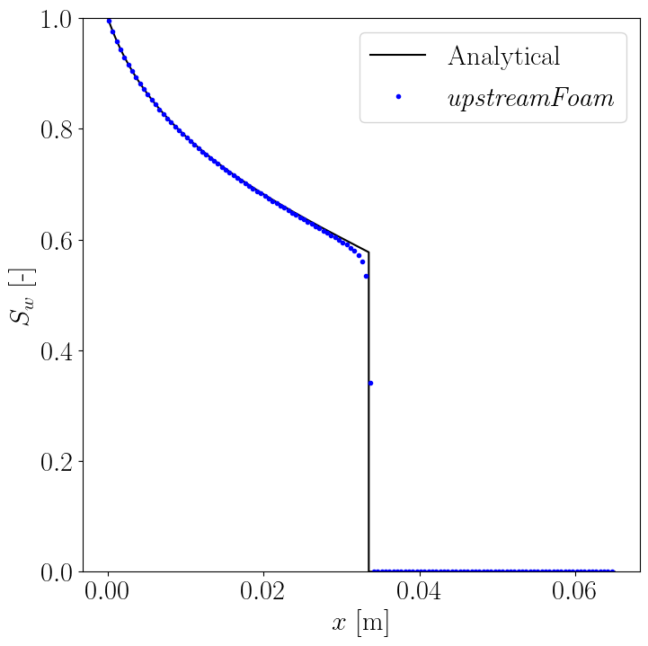
Figure 1: Saturation profile after 1800 s of the homogeneous Buckley-Leverett case.

4.1.2 Heterogeneous Buckley-Leverett

An extension of the previous analysis to flows in one-dimensional heterogeneous porous medium has been introduced in [38], in which the formation consists of a number of domains with different rock properties.

In order to consider the heterogeneous case, we assume that the porosity is $\alpha_{v}=0.2$ if $0\leq x\leq 0.0325$, and $\alpha_{v}=0.1$ if $0.0325<x\leq 0.065$. In the Brooks and Corey relative permeability model, we consider $n=1$ for both phases if $x\leq 0.325$ and $n=4$ for both phases if $x>0.325$. All the other parameters consider the same setup of the previous example.

In Fig. 2 the saturation profile after 1800 s is shown for a computational mesh with 500 cells, where we also note that the approximation is close to the analytical solution for the heterogeneous case.

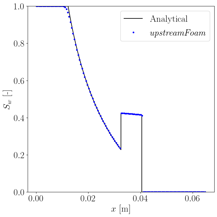
Figure 2: Saturation profile after 1800 s of the heterogeneous Buckley-Leverett case.

4.1.3 Capillary-gravity equilibrium

We now study an air-water incompressible flow in a vertical column (1 m tall) with capillary and gravity effects. The flow is carried out until the gravity-capillarity equilibrium, starting with an initial distribution of the water saturation in a step-wise fashion: the lower half is partially saturated with water ($S_{w}=0.5$ and $S_{a}=0.5$), while the upper half is dry ($S_{w}=0$ and $S_{a}=1$). The bottom boundary condition is a Neumann zero condition, and the top boundary condition is a Dirichlet fixed pressure of 0.1 MPa.

Homogeneous porosity of $\alpha_{v}=0.2$ and absolute permeability of $\mathbf{K}=1\times 10^{-11}\,\mbox{m}^{2}$ are considered. The phase densities are $\rho_{w}=1000\,\mbox{kg/m}^{3}$ and $\rho_{a}=1\,\mbox{kg/m}^{3}$, while the viscosities are $\mu_{w}=0.001\,\mbox{Pa}\cdot\mbox{s}$ and $\mu_{a}=1.76\times 10^{-5}\,\mbox{Pa}\cdot\mbox{s}$. The Brooks and Corey relative permeability model with $n=1$ and $k_{r,i(\max)}=1$ is applied for both phases. Moreover, the capillary pressure is defined through a table filled by the Brooks and Corey correlation using 501 points with parameters $p_{c,0}=1000$ Pa and $\beta=0.5$. The Coats criteria has been applied, with $C_{\max}=0.5$.

Following the analysis proposed in [19, 23], the theoretical steady state can be described as the balance between capillary and gravitational forces, described by

$$\frac{\partial p_{c}}{\partial y}=(\rho_{a}-\rho_{w})g_{y},$$ (33)

where $g_{y}=-10\,\mbox{m}\cdot\mbox{s}^{-1}$ is the gravity in the main flow direction. The expression above can be written as

$$\frac{\partial S_{w}}{\partial y}=\frac{(\rho_{a}-\rho_{w})g_{y}}{\frac{\partial p_{c}}{\partial S_{w}}},$$ (34)

which allows for the calculation of the water saturation gradient according to the chosen capillary pressure model.

The saturation profile at the capillary-gravity equilibrium (after 20000 s) for a computational mesh with 300 cells can be seen in Fig. 3(a). We remark that this case was presented in [19] for the development of the porousMultiphaseFoam toolbox. Therefore, a comparison between both approximations with equivalent numerical setup is included, specifically using the solver impesFoam available in porousMultiphaseFoam. It is possible to note that the obtained saturation profiles are related. A comparison between theoretical and numerical evaluations of the water saturation gradient can be seen in Fig. 3(b), in which we see that both solutions are very similar.

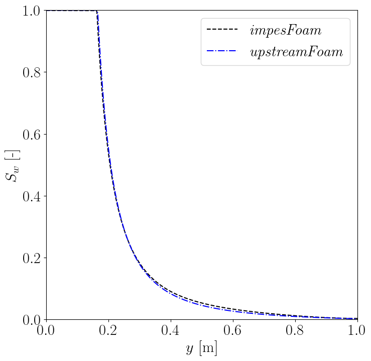
(a) Saturation profile

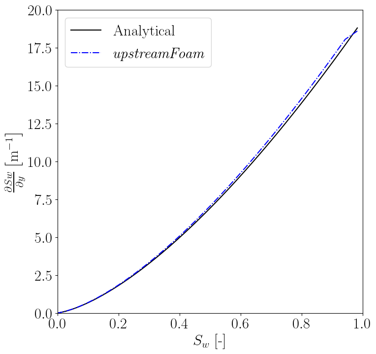
(b) Saturation gradient

Figure 3: Capillary-gravity equilibrium test.

4.1.4 Compressible formation

Since the formation compressibility can significantly influence the reservoir estimations, we propose a simplified verification of the total mass of oil produced in a scenario of depletion generated by compressibility effects. The present experiment considers an oil single-phase flow, however, the upstreamFoam framework performs the computation of both porous and fluid phases.

We study the flow of an incompressible oil in a one-dimensional compressible reservoir of 1000 m long with 100 computational cells. The reservoir, filled with oil, is initially under a pressure of 100 MPa, and a fixed pressure of 10 MPa is maintained at the outlet, resulting in a transient state of oil production by system depletion. The initial porosity, that is, the initial void fraction of the system, is homogeneous, with a value of $\alpha_{v}=0.3$. We consider a constant compressibility of $c_{v}=1\times 10^{-9}\,\mbox{Pa}^{-1}$, absolute permeability of $\mathbf{K}=1\times 10^{-12}\,\mbox{m}^{2}$, oil density of $\rho_{o}=800\,\mbox{kg/m}^{3}$, and oil viscosity of $\mu_{o}=0.002\,\mbox{Pa}\cdot\mbox{s}$. In this experiment, gravity effects are neglected.

Once the porous medium is compressible, the void fraction varies with pressure, and can be described by using a compressibility model, as for example,

$$\alpha_{v}=\alpha_{v,0}\,(1+c_{v}(p_{v}-p_{v,0})),$$ (35)

where $c_{v}$ is the compressibility of the formation, $\alpha_{v,0}$ is the reference porosity, and $p_{v,0}$ is the reference pressure. The above correlation allows for calculating a semi-analytical estimation for the mass balance between the initial and final states of the system.

Considering that the mass of the formation is conserved throughout the depletion process, the initial oil mass is $m^{i}_{o}=\alpha^{i}_{v}\,\rho_{o}\,V$, while the final oil mass is $m^{f}_{o}=\alpha^{f}_{v}\,\rho_{o}\,V$. Therefore, the total mass of oil produced, $m^{p}_{o}$, can be calculated by

$$m^{p}_{o}=m^{i}_{o}-m^{f}_{o}=(\alpha^{i}_{v}-\alpha^{f}_{v})\,\rho_{o}\,V.$$ (36)

Using the linear model of Eq. (35) in Eq. (36), gives the following expression for the total mass of oil produced:

$$m^{p}_{o}=\alpha_{v,0}\,c_{v}(p^{i}_{v}-p^{f}_{v})\,\rho_{o}\,V.$$ (37)

For the simulation parameters considered above, an oil production of $5.4\times 10^{7}$ kg, i.e., 424562.18 STB after depletion is estimated. To evaluate the amount of produced mass of oil during the simulation, we test different values of time step size. The results are reported in Table 1, where it is possible to note that the solver produces adequate results with the error decreasing as the time step decreases.

Time step [s]	Oil produced [STB]	Error [%]
2400	411196.33	3.15
1200	415127.46	2.22
600	418272.36	1.56
300	419844.82	1.09
150	421417.27	0.75

Table 1: Mass of oil produced according to the time step size.

The graph in Fig. 4 illustrates the curve of oil produced for $\Delta t=150$ s. Note that the calculated mass of oil produced approaches the expected value.

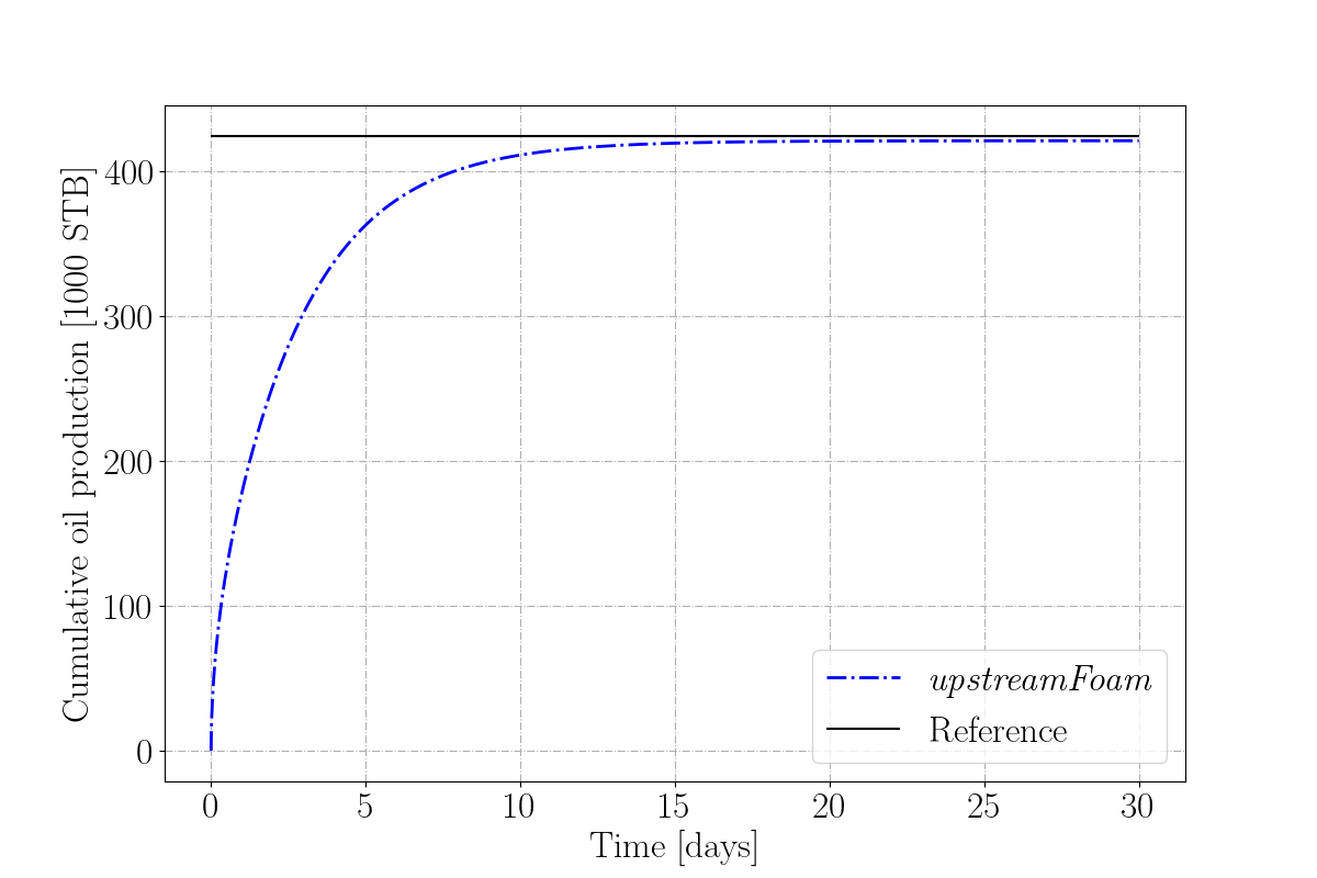
Figure 4: Mass of oil produced by the upstreamFoam with $\Delta t=150$ s.

4.2 2D reservoir problems

This section presents the application of upstreamFoam to approximate two reservoir scale problems. The first experiment shows the evaluation of the head loss of an oil flow in a circular reservoir. The second experiment presents a gas-oil flow in a heterogeneous reservoir with data given by the realistic SPE10 benchmark [37].

4.2.1 Oil flow in a circular reservoir

The head loss of the reservoir is a typical estimate in oil recovery studies. In this experiment, the head loss of a 2D reservoir with oil production by system depletion is investigated.

We simulate the flow of an incompressible oil in a compressible reservoir, given by a circular geometry. The reservoir is initially fully saturated with oil, which is produced through a sink term located in the center of the domain. A fixed pressure of $19.61$ MPa is maintained at the boundaries, along with a constant flow rate at the sink cell. The reservoir, with a diameter of 1000 m, contains an initial homogeneous void fraction of $\alpha_{v}=0.3$. Linear compressibility model is considered with $c_{v}=1\times 10^{-9}\,\mbox{Pa}^{-1}$, absolute permeability of $\mathbf{K}=2\times 10^{-13}\,\mbox{m}^{2}$, oil density of $\rho_{o}=880\,\mbox{kg/m}^{3}$, and oil viscosity of $\mu_{o}=0.002\,\mbox{Pa}\cdot\mbox{s}$. In this experiment, gravity effects are neglected. The Courant time step control is selected with $C_{\max}=0.5$.

Figure 5 shows the pressure profile at time $t=182.64$ days yielded by a simulation with 2053 computational cells. In this case, a flow rate of $2.56\times 10^{-4}\mbox{m}^{3}/\mbox{s}$ was applied at the sink cell, which size is $\Delta x=\Delta y=19.6$ m. From the pressure profile, it is noted that the flow is symmetrical towards the producing cell.

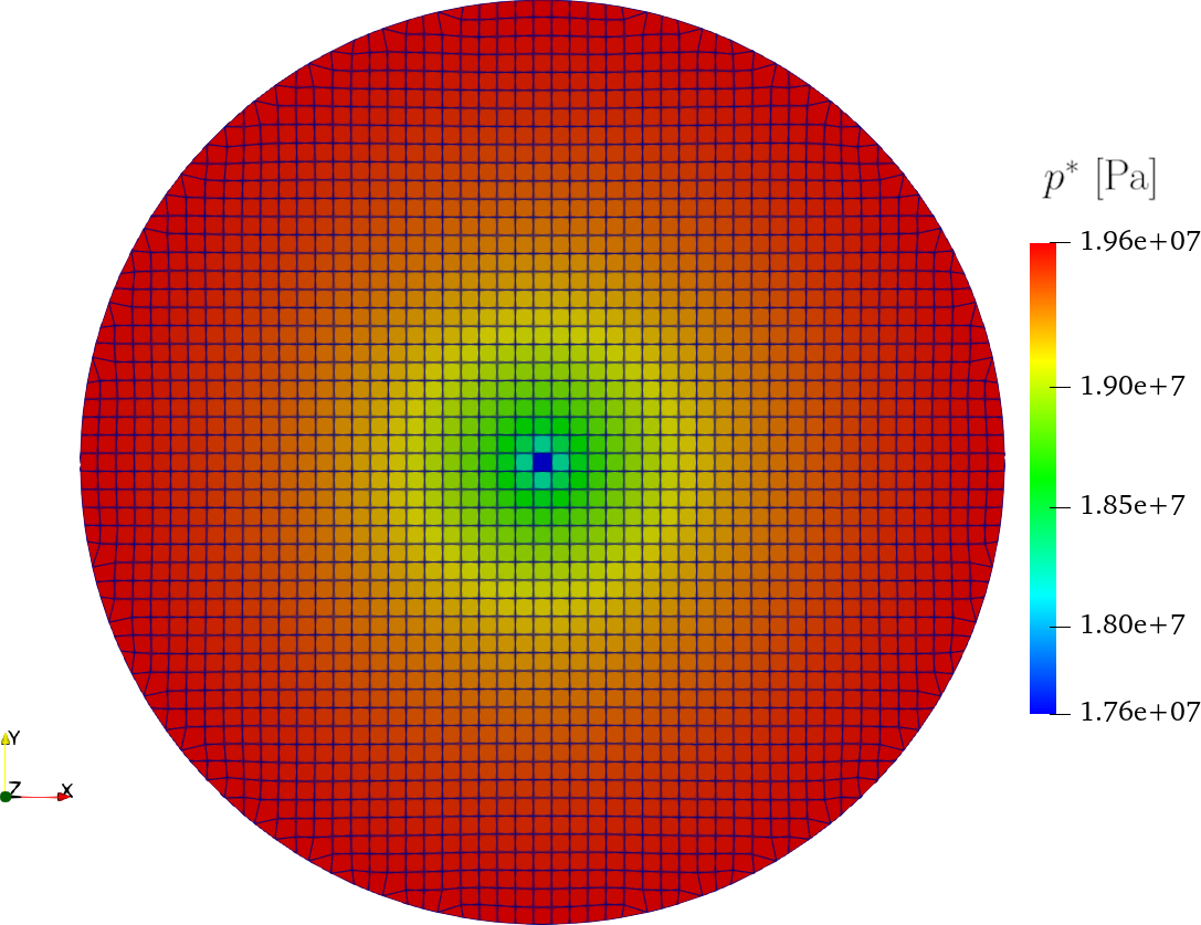
Figure 5: Pressure profile of the 2D reservoir with a sink cell in the center of the domain.

Considering a radial reservoir and using mass conservation and Darcy law for a single-phase flow, one can write

$$\frac{dp}{dr}=-\frac{\mu\,\mathbf{K}^{-1}\rho q}{2\pi rh},$$ (38)

where $r$ is the radius of the reservoir, $q$ is the mass production, $h$ is the height of the sink cell, and $\rho$ is the fluid density [39]. After integrating from the wellbore $r_{w}$ to the reservoir radius $r$, we obtain:

$$\Delta p=-\frac{\mu\,\mathbf{K}^{-1}\rho q}{2\pi h}\ln\left(\frac{r}{r_{w}}\right),$$ (39)

where we set the value of

$$r_{w}=0.20788\sqrt{\Delta x\Delta y},$$ (40)

which represents the equivalent radius derived by Peaceman considering isotropic permeabilities, square grid, single-phase flow, and the well located at the center of an interior cell [40]. Therefore, we are able to estimate the pressure drop between any location in the reservoir and the sink cell by Eq. (39). Figure 6 shows the pressure distribution inside the reservoir presented in Fig. 5 as a function of the diameter, where a total pressure drop of 1.9798 MPa has been obtained. Note that the pressure approximation matches the reference solution.

Once a fixed pressure is applied at the boundaries, the numerical head loss of the system can be computed by using the pressure value in the producer cell. In order to obtain a theoretical head loss of 1.9613 MPa, we set in Eq. (39) the values of $h=1$ m and $\Delta x=\Delta y$. We remark that in this experiment a value of $r=500$ m is considered, and hence, the parameters $r_{w}$ and $q$ vary with the grid size. Table 2 reports the numerical head loss at time $t=182.64$ days obtained by the upstreamFoam considering different grid sizes. The results show that the solver provides accurate estimates of head loss with low errors when compared to the theoretical values.

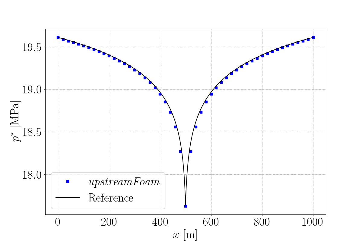
Figure 6: Pressure distribution inside the 2D reservoir as a function of the diameter.

Number of cells [-]	$\Delta x$ [m]	Flow rate [$\mbox{kg}/\mbox{s}$]	$\Delta p$ [MPa]	Error [%]
489	40.7	0.22	1.9826	1.08
2053	19.6	0.19	1.9798	0.94
8021	9.90	0.17	1.9777	0.84
31757	4.08	0.15	1.9763	0.76
126309	2.49	0.14	1.9741	0.65

Table 2: Flow rate imposed and head loss produced according to the grid size.

Lastly, for the same scenario we estimate the numerical head loss of a compressible oil flow, whose density is given by

$$\rho=\frac{\rho_{o,s}+R_{s}\,\rho_{g,s}}{B_{ob}\Big{(}1-c_{o}(p-p_{b})\Big{)}},$$ (41)

where $\rho_{o,s}$ and $\rho_{g,s}$ are the densities of oil and gas at standard conditions, $R_{s}$ is the gas solubility in oil, $B_{ob}$ is the formation volume factor at the bubble point pressure $p_{b}$, and $c_{o}$ is the oil compressibility. Results at time $t=182.64$ days for $\rho_{o,s}=880\,\mbox{kg/m}^{3}$, $\rho_{g,s}=1\,\mbox{kg/m}^{3}$, $R_{s}=199.0$, $B_{ob}=1.4887$, $p_{b}=14.71$ MPa and $c_{o}=1.77\times 10{-9}\,\mbox{Pa}^{-1}$ are shown in Table 3 demonstrating accurate estimates for the head loss, in line with those obtained in the incompressible case.

Number of cells [-]	$\Delta x$ [m]	Flow rate [$\mbox{kg}/\mbox{s}$]	$\Delta p$ [MPa]	Error [%]
489	40.70	0.27	19.86	1.26
2053	19.60	0.23	19.83	1.12
8021	9.90	0.20	19.81	1.02
31757	4.98	0.18	19.80	0.94
126309	2.49	0.16	19.78	0.84

Table 3: Flow rate imposed and head loss produced for the compressible case.

4.2.2 Gas-oil flow in a heterogeneous reservoir

Petroleum reservoirs present high contrast in many proprieties, which impacts the accuracy of the numerical solution and production estimates. This experiment solves a high-contrast heterogeneous reservoir problem with realistic data provided by the SPE10 benchmark [37].

We select the first model, which consists of a two-phase flow (gas and oil) in a 2D vertical cross-sectional geometry whose dimensions are 762 meters long by 7.62 meters wide by 15.24 meters thick, with $100\times 1\times 20$ computational cells. The permeability field of the model is shown in Fig. 7, where the x-axis is plotted using a scale of 0.1 in order to obtain an easily readable representation.

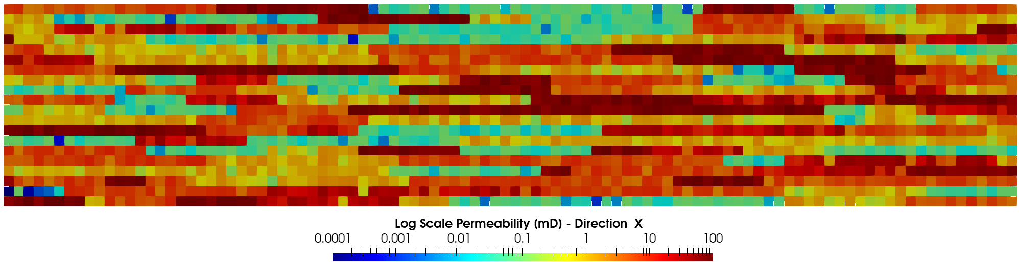
Figure 7: Log-scaled permeability field of the SPE10 project.

An injection-production scenario is considered, where the gas is injected at the left side of the domain (fully saturated with oil), and oil is produced at the right side. Both phases are considered incompressible, while the formation has a compressibility of $c_{v}=6\times 10^{-10}\,\mbox{Pa}^{-1}$ modeled by the linear method with a reference pressure of 689476 Pa, which is the initial pressure at the top of the model at point 0.0 m. The initial void fraction is $\alpha_{v}=0.2$.

The model considers a residual oil fraction of 0.04, that is formulated as a stationary phase fraction in the OpenFOAM framework. Relative permeabilities, illustrated in Fig. 8, are given by the authors in a table. The fluid properties are taken from the SPE10 dataset, that considers the densities $\rho_{o}=700\,\mbox{kg/m}^{3}$ and $\rho_{g}=1\,\mbox{kg/m}^{3}$, and viscosities $\mu_{o}=0.001\,\mbox{Pa}\cdot\mbox{s}$ and $\mu_{g}=0.00001\,\mbox{Pa}\cdot\mbox{s}$. A constant injection rate of $8.0671\times 10^{-5}\mbox{m}^{3}/\mbox{s}$ was applied, along with a production at a constant pressure of 655002 Pa. In this experiment, capillary effects are neglected, and the Courant time step control is selected with $C_{\max}=0.5$.

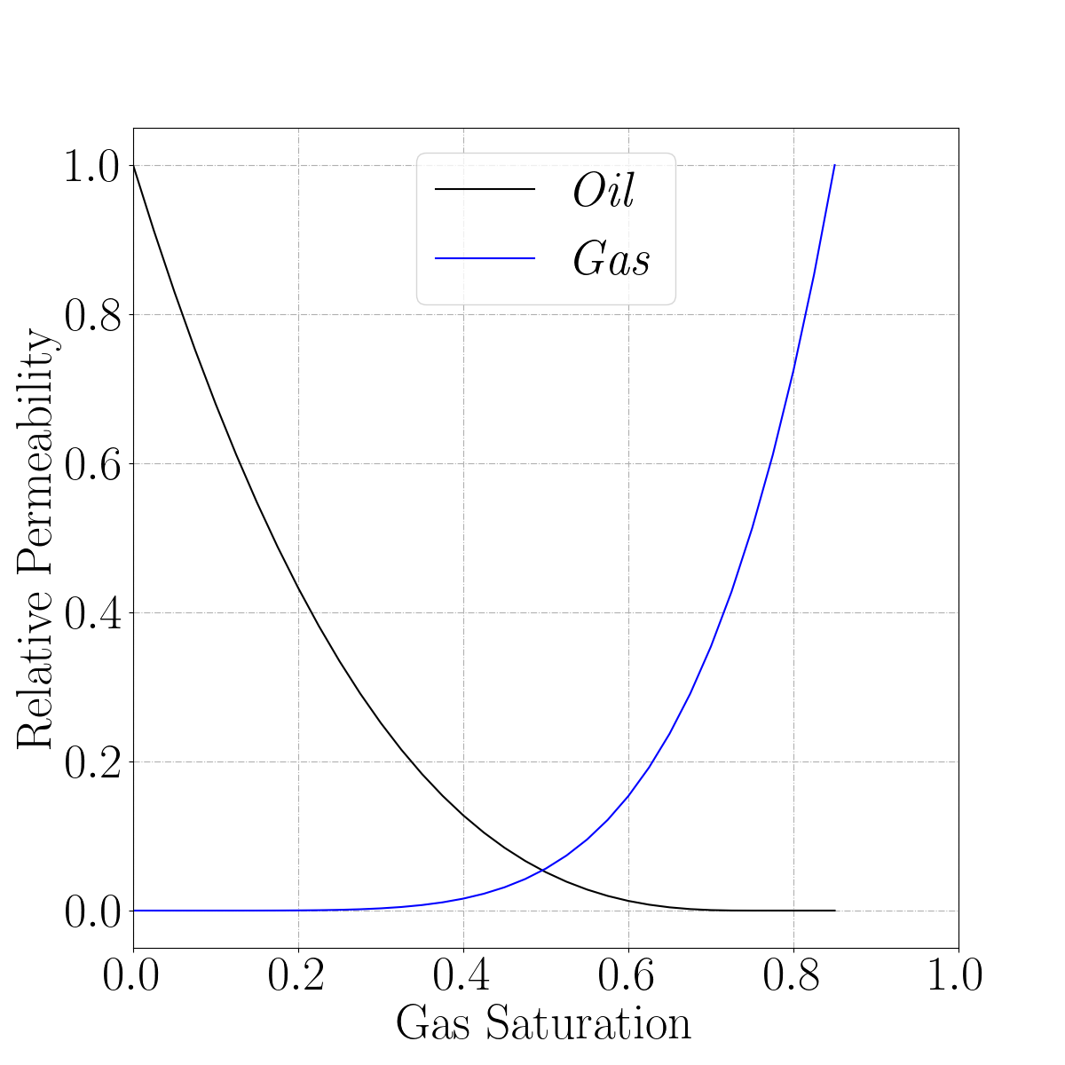
Figure 8: Relative permeabilities for the SPE10 project.

The gas saturation profile after 4800 days can be seen in Fig. 9, where we can note how it flows through the heterogeneous medium. It is possible to observe that gas flows mainly in the superior part of the porous media. This behavior can be justified by the permeability field, presented in Fig. 7.

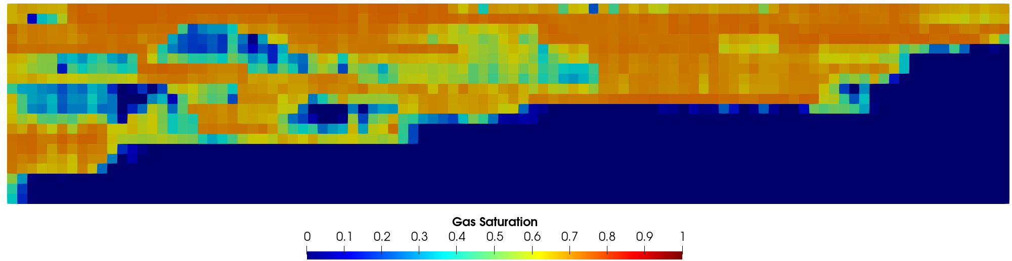
Figure 9: Gas saturation profile after 4800 days.

Figure 10 illustrates the cumulative oil production over a 21-year period (7665 days). The reference result from Landmark [37], obtained using the VIP simulator, is used for comparison. At the initial stages, upstreamFoam exhibits excellent agreement with the reference result. However, after approximately 500 days, upstreamFoam begins to underestimate the cumulative oil production. By 4000 days, it transitions to overestimating the production compared to Landmark’s result. This discrepancy can be attributed to the well injector model, which applies a uniform flow rate across all corresponding cells. It is important to note that wellbore modeling falls outside the scope of this paper; however, it represents a potential avenue for further development and exploration by the authors.

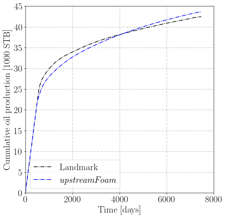
Figure 10: Cumulative oil production.

4.3 Application in a 3D heterogeneous core

Numerical simulations of core flooding experiments are commonly used to validate measurements of rock properties. Therefore, the numerical section is closed with an application of the upstreamFoam in a 3D heterogeneous core simulation.

We consider a manufactured core with a relatively Gaussian distribution of the permeability field, as shown in Fig. 11. The domain, with 25917 computational cells and dimensions of $0.05\,\mbox{m}\times 0.05\,\mbox{m}\times 0.106\,\mbox{m}$, has a homogeneous porosity of $\alpha_{v}=0.2$. The core is saturated with oil and water is injected from left at a constant volumetric rate of $1.66\times 10^{-8}\,\mbox{m/s}$, and the pressure at right is fixed in 0.1  MPa.

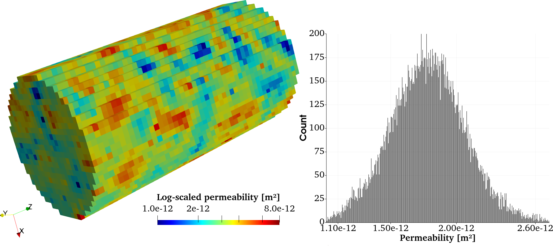
Figure 11: Permeability field of the manufactured core.

In this experiment, gravity and compressibility are neglected. The phase densities are $\rho_{w}=1009\,\mbox{kg/m}^{3}$ and $\rho_{o}=800\,\mbox{kg/m}^{3}$, while the viscosities are $\mu_{w}=0.0005\,\mbox{Pa}\cdot\mbox{s}$ and $\mu_{o}=0.002\,\mbox{Pa}\cdot\mbox{s}$. We first consider a case without capillary pressure and set the Brooks and Corey relative permeability model with $n=1$ and $k_{r,i(\max)}=1$ for both phases. The Coats time step control with $C_{\max}=0.75$ is selected.

The approximations provided by the upstreamFoam and the reference solver impesFoam [19] with an equivalent numerical setup are compared. Figure 12 illustrates saturation profiles obtained by both solvers after 2000 s, showing very similar behaviors.

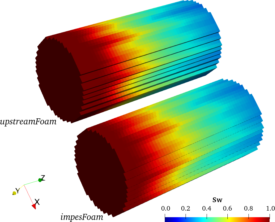
Figure 12: Water saturation profile after 2000 s.

As an illustration of the applicability of the upstreamFoam to more complex systems, we consider the previously test in a three-phase scenario with the oil divided into two phases. The core is initialized with saturation of 0.5 for each oil phase, that share the same fluid properties. The saturations at the center line across the core of the established three-phase flow and previous two-phase flow are presented in Fig. 13. The upstreamFoam produces the same water saturation for both two and three-phase flow regimes, demonstrating consistent results for the same flow condition, independent from the number of phases. We can also confirm that the saturations of both oil phases are equal. In the referred figure, the impesFoam approximation for the two-phase flow is included, which is comparable to the upstreamFoam solution. This study shows that our two-phase flow solution is in agreement with the produced by a reference solver as well as the capability of the upstreamFoam to handle more mobile phases.

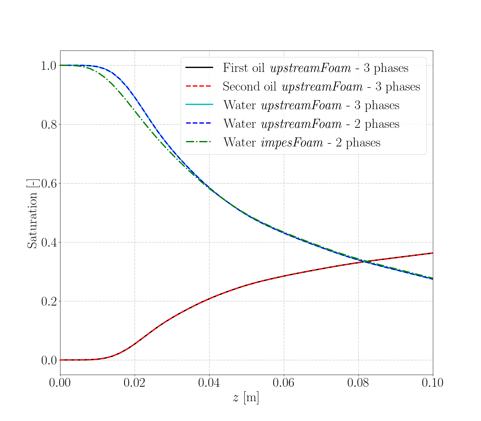
Figure 13: Saturations at 1000 s in a center line across the core.

Our last experiment presents a qualitative study of the upstreamFoam approximation for a case with capillary pressure and more realistic relative permeability curves by comparing our numerical results to the impesFoam solution at equivalent conditions. We consider the same two-phase flow in the 3D core geometry and set the Brooks and Corey model for relative permeability with $n=2$ and $k_{r,i(\max)}=1$ for both phases. The Brooks and Corey model for the capillary pressure with $\beta=0.5$ and $p_{c,0}=10$ Pa is chosen.

Figure 14(a) shows that the simulations performed with upstreamFoam and impesFoam develop similar saturation profiles. The same time step Coats restriction has been set for both solvers, which presented similar time step histories, as reported in Fig. 14(b). We remark that the restricted time step sizes presented are close related to the capillary effects, that in this case are are not too strong due to the choice of $p_{c,0}$. Other temporal discretizations, such as implicit treatments, can be considered to overcome such limitations.

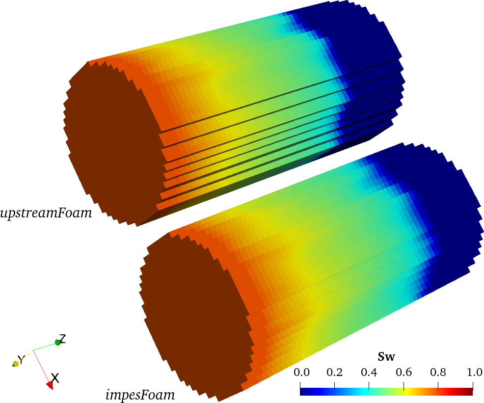
(a) Saturation profiles

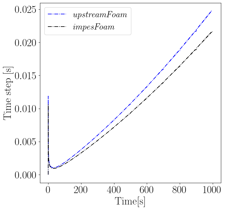
(b) Time step history

Figure 14: Water saturation profile after 1000 s and time step history for the case with capillary pressure and quadratic relative permeability curves.

5 Conclusions

In this work, we introduced and tested a new OpenFOAM application to simulate multiphase flows in porous media. The solver, called upstreamFoam, combines the Eulerian multi-fluid formulation for a system of phase fractions with Darcy’s law for flows through porous media. It is based on the multiphaseEulerFoam and includes models for reservoir simulation of the porousMultiphaseFoam, taking advantage of the most recent technologies developed for these well-established solvers.

The upstreamFoam has been successfully tested in a wide range of multiphase flows in porous media. We verified the solver simulating classical problems with analytical, semi-analytical, and reference solutions given by the porousMultiphaseFoam. Studies with different data and geometries have been performed to evaluate reservoir properties estimates, resulting in satisfactory accuracy. We also have demonstrated the potential of the solver to approximate complex problems in a multiphase scenario with more than two mobile phases.

The presented solver was developed in a general formulation, that can be extended to multiple species, mass transfer, and others complexities employing the tool-set, capabilities, and efficiency offered by the OpenFOAM framework. In future works, we intend to include wellbore models and investigate the use of new schemes to overcome the time step restrictions.

References

- [1] D. B. Spalding, Numerical computation of multi-phase fluid flow and heat transfer, In Von Karman Inst. for Fluid Dyn. Numerical Computation of Multi-Phase Flows (1981) 161–191.
- [2] H. Jasak, Error analysis and estimation for the finite volume method with applications to fluid flows., Ph.D. thesis, Imperial College London (University of London) (1996).
- [3] H. G. Weller, G. Tabor, H. Jasak, C. Fureby, A tensorial approach to computational continuum mechanics using object-oriented techniques, Computers in physics 12 (6) (1998) 620–631.
- [4] D. P. Hill, The computer simulation of dispersed two-phase flow, Ph.D. thesis, Citeseer (1998).
- [5] M. Ishii, T. Hibiki, Thermo-fluid dynamics of two-phase flow, Springer Science & Business Media, New York, 2010.
- [6] C. Crowe, M. Sommerfeld, Y. Tsuji, et al., Multiphase flows with droplets and particles, CRC Press - Taylor & Francis Group, Boca Raton, FL, 1998.
- [7] D. A. Drew, S. L. Passman, Theory of multicomponent fluids, Vol. 135, Springer Science & Business Media, Berlin, 2006.
- [8] H. G. Weller, Derivation, modelling and solution of the conditionally averaged two-phase flow equations, Nabla Ltd, No Technical Report TR/HGW 2 (2002) 9.
- [9] H. Rusche, Computational fluid dynamics of dispersed two-phase flows at high phase fractions, Ph.D. thesis, Imperial College London (University of London) (2003).
- [10] L. F. L. Silva, R. Damian, P. L. Lage, Implementation and analysis of numerical solution of the population balance equation in CFD packages, Computers & Chemical Engineering 32 (12) (2008) 2933–2945.
- [11] L. F. L. Silva, P. L. Lage, Development and implementation of a polydispersed multiphase flow model in OpenFOAM, Computers & chemical engineering 35 (12) (2011) 2653–2666.
- [12] J. L. Favero, L. F. L. Silva, P. L. Lage, Modeling and simulation of mixing in water-in-oil emulsion flow through a valve-like element using a population balance model, Computers & Chemical Engineering 75 (2015) 155–170.
- [13] K. E. Wardle, H. G. Weller, Hybrid multiphase CFD solver for coupled dispersed/segregated flows in liquid-liquid extraction, International Journal of Chemical Engineering 2013 (2013).
- [14] H. G. Weller, A new approach to VOF-based interface capturing methods for incompressible and compressible flow, OpenCFD Ltd., Report TR/HGW 4 (2008) 35.
- [15] F. Tocci, Assessment of a hybrid VOF two-fluid CFD solver for simulation of gas-liquid flows in vertical pipelines in OpenFOAM, Master’s thesis, Politecnico di Milano, Italy (2016).
- [16] J. Bear, Dynamics of fluids in porous media, Courier Corporation, New York, 1988.
- [17] K. Aziz, Petroleum reservoir simulation, Applied Science Publishers 476 (1979).
- [18] Z. Chen, G. Huan, Y. Ma, Computational methods for multiphase flows in porous media, SIAM, Philadelphia, PA, 2006.
- [19] P. Horgue, C. Soulaine, J. Franc, R. Guibert, G. Debenest, An open-source toolbox for multiphase flow in porous media, Computer Physics Communications 187 (2015) 217–226.
- [20] L. Sugumar, A. Kumar, S. K. Govindarajan, Grid adaptation of multiphase fluid flow solver in porous medium by OpenFOAM, Petroleum & Coal 62 (4) (2020).
- [21] S. Fioroni, A. E. Larreteguy, G. B. Savioli, An OpenFOAM application for solving the black oil problem, Mathematical Models and Computer Simulations 13 (5) (2021) 907–918.
- [22] P. Horgue, F. Renard, G. S. Gerlero, R. Guibert, G. Debenest, porousmultiphasefoam v2107: An open-source tool for modeling saturated/unsaturated water flows and solute transfers at watershed scale, Computer Physics Communications 273 (2022) 108278.
- [23] F. J. Carrillo, I. C. Bourg, C. Soulaine, Multiphase flow modeling in multiscale porous media: An open-source micro-continuum approach, Journal of Computational Physics: X 8 (2020) 100073.
- [24] A. Sangnimnuan, J. Li, K. Wu, Development of coupled two phase flow and geomechanics model to predict stress evolution in unconventional reservoirs with complex fracture geometry, Journal of Petroleum Science and Engineering 196 (2021) 108072.
- [25] M. Muskat, Physical principles of oil production, McGraw-Hill, New York, 1981.
- [26] K. H. Coats, A note on IMPES and some IMPES-based simulation models, SPE Journal 5 (03) (2000) 245–251.
- [27] R. Keser, M. Battistoni, H. G. Im, H. Jasak, A Eulerian multi-fluid model for high-speed evaporating sprays, Processes 9 (6) (2021) 941.
- [28] H. Wang, H. Wang, F. Gao, P. Zhou, Z. J. Zhai, Literature review on pressure–velocity decoupling algorithms applied to built-environment CFD simulation, Building and Environment 143 (2018) 671–678.
- [29] S. M. Damián, N. M. Nigro, An extended mixture model for the simultaneous treatment of small-scale and large-scale interfaces, International Journal for Numerical Methods in Fluids 75 (8) (2014) 547–574.
- [30] M. Rudman, Volume-tracking methods for interfacial flow calculations, International journal for numerical methods in fluids 24 (7) (1997) 671–691.
- [31] R. Courant, K. Friedrichs, H. Lewy, Über die partiellen differenzengleichungen der mathematischen physik, Mathematische annalen 100 (1) (1928) 32–74.
- [32] J. Franc, P. Horgue, R. Guibert, G. Debenest, Benchmark of different CFL conditions for IMPES, Comptes Rendus Mécanique 344 (10) (2016) 715–724.
- [33] K. Coats, IMPES stability: selection of stable timesteps, SPE Journal 8 (02) (2003) 181–187.
- [34] R. H. Brooks, Hydraulic properties of porous media, Ph.D. thesis (1965).
- [35] M. Leverett, Capillary behavior in porous solids, Transactions of the AIME 142 (01) (1941) 152–169.
- [36] D. N. Nguyen, K. S. Jung, J. W. Shim, C. S. Yoo, Real-fluid thermophysicalmodels: An OpenFOAM-based library for reacting flow simulations at high pressure, Computer Physics Communications 273 (2022) 108264.
- [37] M. A. Christie, M. J. Blunt, Tenth SPE comparative solution project: A comparison of upscaling techniques, SPE Reservoir Evaluation & Engineering 4 (04) (2001) 308–317.
- [38] Y.-S. Wu, Multiphase fluid flow in porous and fractured reservoirs, Gulf professional publishing, Waltham, MA, 2015.
- [39] Z. Chen, Y. Zhang, Well flow models for various numerical methods., International Journal of Numerical Analysis & Modeling 6 (3) (2009).
- [40] D. W. Peaceman, Interpretation of well-block pressures in numerical reservoir simulation (includes associated paper 6988), Society of Petroleum Engineers Journal 18 (03) (1978) 183–194.