EZClone: Improving DNN Model Extraction Attack via Shape Distillation from GPU Execution Profiles

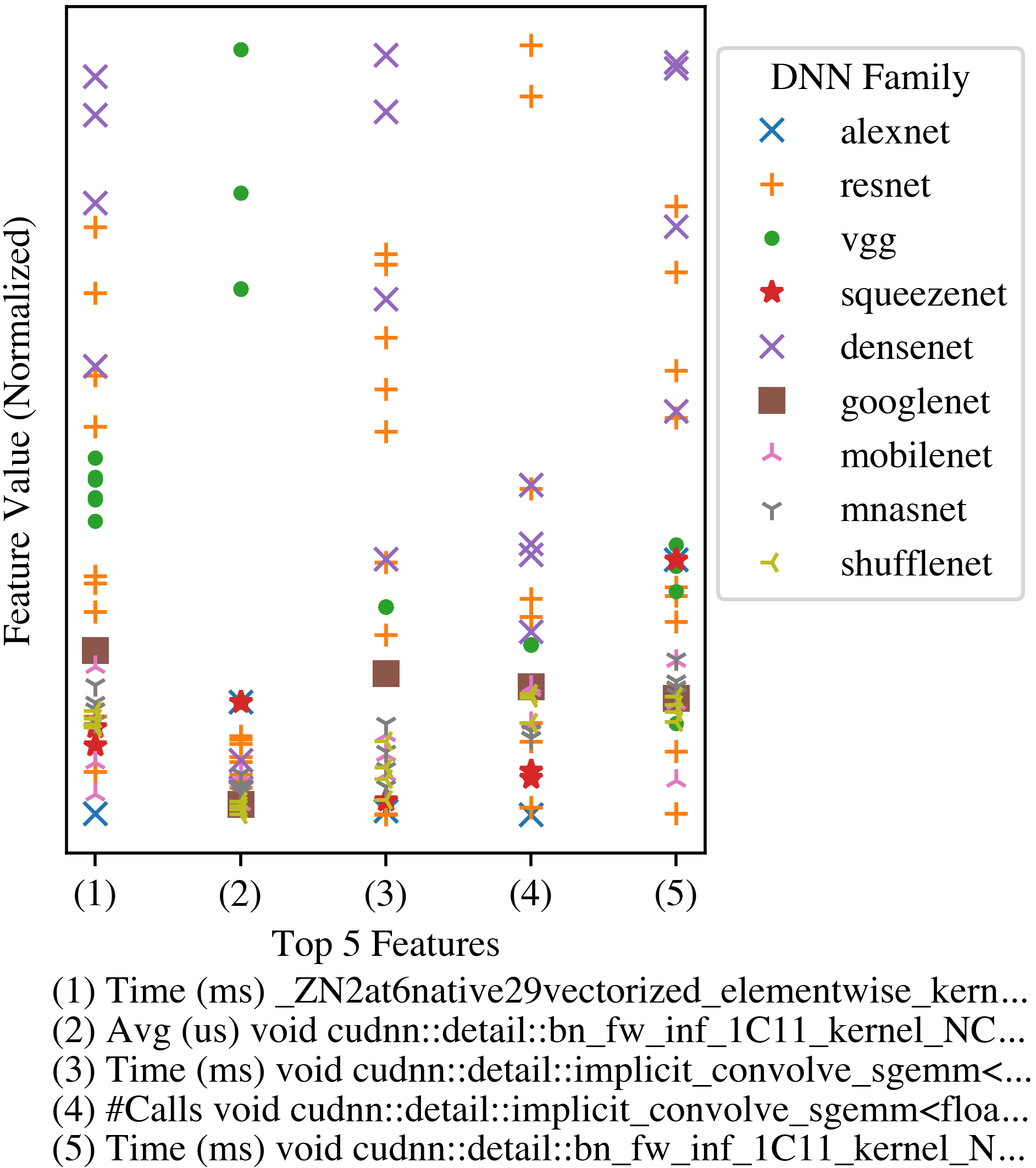
Figure 1: GPU kernel feature values for all 36 PyTorch vision architectures by architecture family. Values are averaged over 50 profiles and normalized. The features are ranked from the set of non-memory related GPU kernels using Recursive Feature Elimination on a Random Forest model, which achieves 100% architecture prediction accuracy using the top 3 features.

Abstract

Deep Neural Networks (DNNs) have become ubiquitous due to their performance on prediction and classification problems. However, they face a variety of threats as their usage spreads. Model extraction attacks, which steal DNNs, endanger intellectual property, data privacy, and security. Previous research has shown that system-level side-channels can be used to leak the architecture of a victim DNN, exacerbating these risks. We propose two DNN architecture extraction techniques catering to various threat models. The first technique uses a malicious, dynamically linked version of PyTorch to expose a victim DNN architecture through the PyTorch profiler. The second, called EZClone, exploits aggregate (rather than time-series) GPU profiles as a side-channel to predict DNN architecture, employing a simple approach and assuming little adversary capability as compared to previous work. We investigate the effectiveness of EZClone when minimizing the complexity of the attack, when applied to pruned models, and when applied across GPUs. We find that EZClone correctly predicts DNN architectures for the entire set of PyTorch vision architectures with 100% accuracy. No other work has shown this degree of architecture prediction accuracy with the same adversarial constraints or using aggregate side-channel information. Prior work has shown that, once a DNN has been successfully cloned, further attacks such as model evasion or model inversion can be accelerated significantly.

1 Introduction

Deep Neural Networks (DNNs) have risen to the forefront of intelligent technological deployments due to their sublime performance on cognitive prediction and classification problems. DNNs have broken boundaries in areas including image classification [22, 43], speech recognition [49], natural language processing [44, 46, 40], and continue to pervade into new problem domains. The predominant and emerging business model for AI providers to monetize these networks is to license their use, charge for each query to the model, or deploy the model onto edge computing platforms. This business model, which views DNNs as intellectual property [35], necessitates the protection of the DNN against theft. However, the model extraction attack [45, 25, 50], which enables an adversary to steal a DNN, has been shown to be effective in many different attacking scenarios. AI providers are invested in preventing model extraction attacks for the following reasons:

1. Producing a high-quality DNN is expensive [41, 42]. First, the provider must collect, validate, maintain, and (in the case of sensitive data) protect a large dataset. In the era of big data, these datasets may be Petabytes in scale [18]. Second, the provider must design or choose a preexisting DNN architecture. Designing an architecture is an active research area [7] and involves a team of scientists combining experience, ingenuity, and vast experimentation. Third, the provider must train the model. For example, the cost to train a 1.5 billion parameter language model ranges from $80k to $1.6m [42].

2. Stolen DNNs present several threats. An adversary motivated by theft possesses the capability to dismantle the AI provider’s business model by evading paywalls, selling intellectual property as their own, or releasing models to the public. An adversary motivated by reconnaissance can use the stolen model to mount further attacks [6, 2, 1], such as model inversion, which can recover data used to train the DNN, and model evasion, which allows the adversary to trick the DNN into undesired behavior. These attacks raise privacy, ethical, and legal concerns.

These risks motivate proactive discovery of the exploits that enable model extraction attacks.

Model extraction involve two steps. Architecture extraction [55, 16, 26, 28, 47] determines the architecture of the victim model, and parameter extraction [12, 54, 53, 19, 4, 9, 33] recovers the weights and biases of the victim model. This work focuses on architecture extraction. Parameter extraction methods typically assume that the architecture extraction step has already been completed.

Various system-level side-channels have been shown to leak the victim model architecture [25, 27, 5], including cache usage of the CPU [51, 15, 24] and GPU [36, 28], memory access patterns of the CPU [20, 16], GPU [23, 16], and DNN accelerators [17], GPU kernel profiles [16, 55, 28, 47, 20, 36], power consumption [20, 48], and electromagnetic emanations [52, 26, 3, 8]. Due to the computational complexity of state-of-the-art DNNs, they are often deployed on GPUs to speedup matrix multiplication operations that account for most of the workload. This makes GPU side-channel attacks particularly pertinent.

Using the side channel information, the victim model architecture may be predicted in one shot [36, 20, 48, 52], reconstructed layer-by-layer [15, 51, 16, 26, 17], or inferred [55] if there is adequate information. These existing approaches have several weaknesses. Architecture prediction methods predict the victim architecture from a candidate set of architectures, and thus are limited by the size of that set and struggle to distinguish between similar architectures [20, 36]. However, a correct prediction extracts the architecture exactly. Architecture reconstruction methods are not limited to a candidate set of architectures, but 1) are limited to a candidate set of layer types, 2) struggle to extract irregular architectures with complex/rare layers and connections [16, 26], and 3) do not extract the victim architecture exactly. Architecture inference methods gather enough information to infer the victim architecture, but at the cost of assuming a stronger adversary.

In response to these weaknesses, we propose EZClone, a simple, low-cost, and accurate architecture prediction method which is not limited to a small candidate set and is capable of distinguishing between similar architectures. In fact, we show that EZClone can recover all 36 PyTorch vision architectures [37] with 100% accuracy, using as little as 3 GPU kernel features found through empirical analysis, takes less than 1 minute per architecture, and works on pruned DNNs. No other work has demonstrated exact architecture extraction over such a large and diverse set of architectures. Table 1 shows a comparison of EZClone to existing work. The DeepPeep attack [20] can predict DNN architecture family using 3 hand-selected GPU kernel features, but requires side-channel information during victim model training and cannot distinguish between DNN architectures of the same family using GPU kernel features alone.

EZClone is the only GPU profile architecture extraction approach that uses exclusively aggregate, rather than time-series, side-channel information collected during victim DNN execution, and EZClone is the highest performing attack that uses an aggregate data regardless of the side-channel medium. Previous work has suggested that, to defend against time-series based attacks, a defender could limit the granularity of access to time-series information [28] or reorder DNN execution [15, 16, 3]. However, the efficacy of EZClone demonstrates that the attacker may circumvent a defense of these types because time-series information is not required. This motivates a paradigm shift in defense approaches.

In addition to EZClone, we present another architecture extraction method in which an adversary may substitute a malicious version of the PyTorch library during dynamic loading. The malicious library is functionally equivalent to PyTorch except that the PyTorch profiler is enabled. We propose a parser that reads PyTorch profiles and automatically generates the PyTorch code for the victim DNN architecure.

Our contributions include:

1. A high performance, low-cost architecture prediction framework capable of predicting all PyTorch vision architectures with 100% accuracy, using as few as 3 GPU kernel features.

2. An analysis of the efficacy of this framework between the Nvidia Tesla T4 and Nvidia Quadro RTX 8000 GPUs and on pruned DNN models.

3. A systematic analysis of GPU feature importance as it relates to DNN architecture.

4. Another architecture extraction framework using a malicious, dynamically loaded version of the PyTorch library and capable of generating PyTorch code for the victim DNN architecture.

Related Work	Assumed Adversary Capability				Attack Requirements
	Local Access	Snoop PCIe	Attack During Training	CPU/GPU Share Memory	Extraction Type	Memory Data	Time Series Data
Hu, et al. [16]	✔	✔	✗	✗	Reconstruct	✔	✔
Zhu et al. [55]	✔	✔	✗	✗	Infer	✗	✔
Naghibijouybari et al. [28]	✗	✗	✔	✗	N/A	✔	✔
Wei et al. [47]	✗	✗	✔	✗	Reconstruct	✔	✔
Kumar Jha et al. [20]	✗	✗	✔	✗	Predict	✔	✗
Patwari et al. [36]	✗	✗	✗	✔	Predict	✔	✔
Our Work (EZClone)	✗	✗	✗	✗	Predict	✗	✗

Table 1: Comparison with related works which also use GPU profiles as a side-channel. Other than [20], all works use time-series side-channel information, although [20] augments their aggregate GPU profile data with power time-series data. Most works augment their side-channel information with additional memory data, such as the volume of cache/DRAM read/write requests and the amount of free memory. Naghibijouybari et al. [28] do not complete architecture extraction and only predict the number of neurons in a DNN.

2 Background

2.1 Deep Neural Networks

In this work, we consider feed-forward neural networks performing classification tasks. The architecture of a DNN specifies its computational graph and refers to the layer and connections that compose this graph. There are different layer types, such as fully connected, convolution, or batch norm, and different layer hyperparameters, such as number of nodes, stride length, and padding. The connections represent how the layers are linked together in the graph. We denote an architecture as $f$ and a model as $f^{\theta}$, which is an architecture parameterized by $\theta$, the parameters found through a training process, including weights, biases, and batch normalization parameters. The training hyperparameters, such as learning rate, batch size, and number of training epochs, are not represented in the model. The output of the model $f^{\theta}(x)$ for an input $x\in\mathcal{X}$ is a categorical distribution among the $k$ classes.

DNN pruning: Pruning [14] is a DNN optimization technique aimed at reducing the amount of operations necessary to execute an inference by removing the least important parameters from the set of all parameters $\theta$. In effect, this removes connections in a DNN resulting in a sparser network, and is functionally equivalent to setting the least important parameters to 0. Pruning has been shown to significantly reduce the size of the network while incurring little to no accuracy loss [14].

Type	Name	Time(%)	Time (ms)	Calls	Avg (us)	Min (us)	Max (ms)
GPU kernel	void cudnn::detail::implicit_convolve	44.39	12.80	370	34.61	14.56	0.06
	volta_scudnn_winograd_128x128_ld	19.08	5.50	190	28.97	9.86	0.07
	[CUDA memcpy HtoD]	17.08	4.93	356	13.84	0.83	0.97
	void cudnn::detail::bn_fw_inf_1C11_	5.27	1.52	570	2.67	1.66	0.01
API call	cudaMemcpyAsync	86.69	5375.96	364	14769.12	3.85	5361.14
	cudaFree	8.12	503.67	7	71952.31	0.62	290.23
	cudaMalloc	3.80	235.47	35	6727.72	5.45	232.20
Device	System Signal	Sample Count			Avg	Min	Max
Quadro RTX 8000	SM Clock (MHz)	66			1378.41	300	1395
	Memory Clock (MHz)	66			6407.65	405	6500
	Temperature (C)	131			44.98	44	46
	Power (mW)	131			63235.14	31024	72179

Table 2: Partial Data from an aggregated profile of an application running 10 inferences on a GoogleNet model trained on ImageNet on an Nvidia Quadro RTX 8000 GPU. Full profile data would include $\sim$15 GPU kernels, $\sim$30 API calls, and 5 system signals. GPU kernel names are truncated to fit in the table. A convolution operation called in PyTorch code will invoke the GPU kernel void cudnn::detail::implicit_convolve.

2.2 White-Box vs Black-Box Access

An adversary with white-box access to a model $f^{\theta}$ has full information of both the architecture $f$ and the parameters $\theta$ of the model. On the other hand, an adversary with black-box or query access to a model $f^{\theta}$ has no knowledge of the model architecture and the model parameters. They may only query the model by providing an input $x\in\mathcal{X}$ and observe the output $f^{\theta}(x)$, a categorical distribution among the $k$ classes. From an adversarial perspective, white-box access is much more valuable than black-box access. The adversary will be able to calculate the gradient of the model, which improves the efficacy and reduces the cost of adversarial attacks.

2.3 Model Extraction Attack

A model extraction attack steals a black-box victim model $f_{v}^{\theta}$. To do this, an adversary constructs a surrogate model $f_{s}^{\theta^{\prime}}$, to which they will have white-box access. The goal is to construct the surrogate model to be as close to the victim model as possible. In the ideal case the adversary achieves exact replication where 1) $f_{s}=f_{v}$ (the surrogate and victim have the same architecture) and 2) $\theta^{\prime}=\theta$ (the surrogate and the victim have the same parameters). In practice, there is a tradeoff between the attack complexity/adversarial capability and the similarity between the victim and surrogate models.

To address the first objective, ($f_{s}=f_{v}$) the adversary conducts architecture extraction in which an architecture prediction or reconstruction algorithm $\mathcal{A}$ predicts the architecture of the victim model based on side-channel information $\mathcal{H}(f_{v}^{\theta})$ collected about the victim model. Formally $\mathcal{A}$ performs the function

$$\mathcal{A}(\mathcal{H}(f_{v}^{\theta}))=\mathbb{E}[f_{v}|\mathcal{H}(f_{v}^{\theta})]=\hat{f}_{v}$$ (1)

where $\hat{f}_{v}$ is the predicted architecture of the victim model. Typically, $\mathcal{A}$ is a machine learning model trained on a dataset of side-channel information collected on a training set of DNN architectures. The burden of creating this dataset and selecting the training architectures is on the adversary.

If $\mathcal{A}$ is a prediction algorithm, then the predicted architecture $\hat{f_{v}}$ is limited to a candidate set of architectures $C=\{f_{c_{1}},f_{c_{2}},...f_{c_{n}}\}$. For each candidate architecture $f_{c_{i}}\in C$, the adversary will collect $N$ profiles $\mathcal{H}(f_{c_{i}}^{\theta_{i}})$ forming a labeled dataset of profiles of that architecture $S_{i}=\{\mathcal{H}(f_{c_{i}}^{\theta_{i}}),f_{c_{i}}\}^{N}$ where the data is the profile and the label is the architecture. These are combined to form a dataset over all the candidate architectures $D=\bigcup_{i}S_{i}$ which is the training data for $\mathcal{A}$. On the other hand, if $\mathcal{A}$ is a reconstruction algorithm, the the labels in $D$ will be a sequence of layer types instead of an architecture, and instead of predicting the full victim architecture, $\mathcal{A}$ will predict layers of the architecture one at a time. Since DNN layers are executed sequentially, this requires time-series side channel information $\mathcal{H}(f_{v}^{\theta})$. The layer hyperparameters (for example, convolution kernel size) and connections are added as a second step.

To address the second objective ($\theta^{\prime}=\theta$), the adversary instantiates a surrogate model $f_{s}^{\theta^{\prime}}$ with $f_{s}=\hat{f}_{v}$ and runs a parameter extraction algorithm so that $\theta^{\prime}\approx\theta$. The problem of parameter extraction has been extensively studied [12, 54, 53, 19, 4, 9, 33] and is not the focus of this work, although it is important to note that many state-of-the-art parameter extraction algorithms assume that the victim architecture has already been found.

2.4 NVIDIA Profiler

nvprof [31] is a command-line tool developed for Nvidia GPUs to profile CUDA activites. CUDA is Nvidia’s API to the GPU instruction set. When running a DNN application on an Nvidia GPU, high-level code (e.g. in PyTorch) makes calls to the CUDA API, which will translate these calls into GPU kernels (compiled CUDA routines, like convolution) to run on the GPU. nvprof monitors the application’s GPU kernel invocations (type of invocation and time spent on the invocation), as well as memory operations (such as program counters of allocations/frees and time/type of memory operations, such as copy from host to device or device to host) and system level information (clock speed, power consumption, and thermal data). All of this information is compiled into a report called a profile of the application.

nvprof may be configured to generate profiles in time series or aggregate mode. Time series mode records the order that the GPU kernels and memory operations were completed, along with the time taken for each. Time series nvprof profiles has been demonstrated as an effective side-channel $\mathcal{H}(f^{\theta}_{v})$ to leak victim model DNN architecture [16, 55, 20], and to facilitate workload characterization of processes running on the GPU [56]. On the other hand, aggregate mode monitors the time spent on each GPU kernel/memory operation over the entire program’s computation. Aggregate mode loses the ordering of kernel calls but enables the analysis of kernel signals as a distribution; for each GPU kernel, nvprof reports the number of calls, time spent on all calls, avg/min/max time spent on a call, and percentage of total time spent on that GPU kernel. Table 2 displays a portion of an aggregated GPU Profile generated by nvprof on an application running 10 inferences on GoogleNet. Each datapoint of the profile, such as the time($\%$), time(ms), calls, avg(us), min(us), and max(ms) of GPU kernels and API calls, as well as the data from the system signals, becomes a feature of the side-channel information $\mathcal{H}(f^{\theta})$. Prior work [20] has demonstrated a relationship between salient features of this aggregate side-channel information and DNN architecture.

From the adversary’s point of view, nvprof has several advantages. First, nvprof does not require physical access to a device to generate a profile. Second, nvprof is agnostic of the application format; the application may take the form of a plaintext source code file or a binary executable file that hides source code. This enables an adversary to collect profiles on applications which have obfuscated the source code and data. Third, nvprof is passive, meaning that the victim application is agnostic to whether or not nvprof is running. This makes detecting and preventing the attack more difficult.

The biggest drawback to nvprof is that it requires administrator privileges. However, is not a prohibitive requirement. If the victim application is deployed as a binary executable which may occur in licensed or pay-per-query business models, then the application runs on the adversary’s machine, where they have administrator privileges. If the victim application is deployed on an edge device, then malicious system administrators will have the potential to run nvprof. Finally, nvprof has an option to disable the administrator priviledge requirement, and this configuration switch may be enabled on some systems.

2.5 PyTorch Profiler

The PyTorch Profiler [39] is intended to aid developers in the performance analysis of DNNs implemented in PyTorch. Enabling the profiler is a simple matter of inserting a code wrapper around the Python method that calls the model’s inference. The parser may be configured to output a JSON file containing a detailed trace of GPU and CPU operations executed in the inference process. In a non-adversarial setting, a developer would use this trace file as input to a Visualization Tool like Tensorboard [11], which mainly focuses on performance analysis, and provides functionality for visualizing DNN architectures based on profile data.

The elements in the output trace file contain enough information to reconstruct the architecture of a DNN. An attacker with access to this trace can devise a simple parser that would take this information and output PyTorch code equivalent to the original, which can then be used to train a surrogate model using parameter extraction methods. This architecture extraction method poses a threat when the attacker does not have access to the model itself, which might be protected under encryption, but the PyTorch API itself is not protected, allowing the adversary to enable the PyTorch Profiler and access the trace file. This work proposes a parser for the trace file that outputs PyTorch code implementing the DNN architecture.

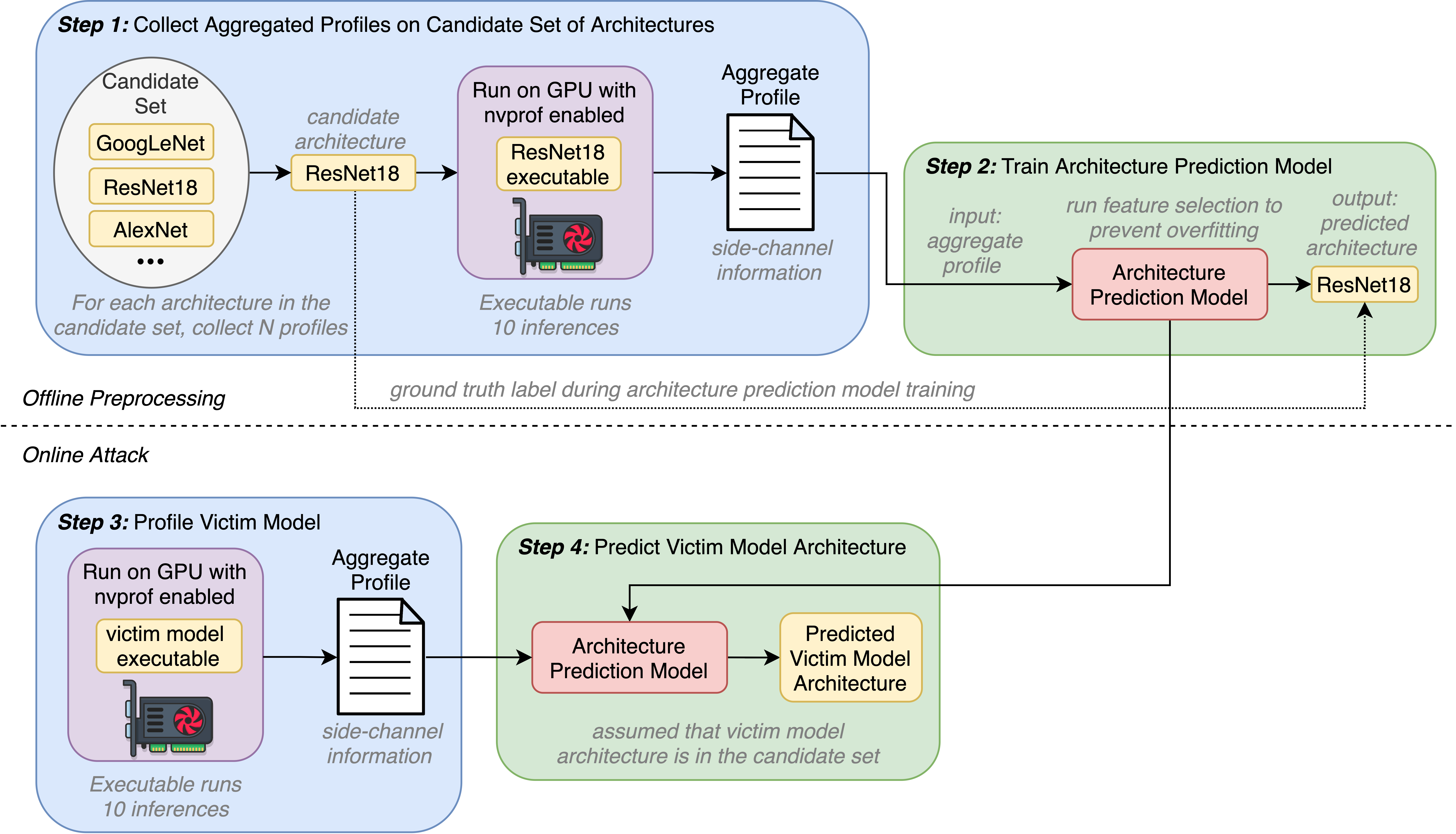
Figure 2: EZClone attack framework.

3 Threat Model

Adversary’s Objective: The adversary wants to run an accurate and inexpensive model extraction attack. To do this, they must complete architecture extraction then parameter extraction. EZClone focuses only on architecture extraction. After running EZClone and extracting the architecture, the adversary may choose a parameter extraction method to complete the model extraction attack. From there, the adversary may exploit the extracted surrogate model by bypassing paywalls, selling the model, or releasing the model. Additionally, since the adversary gains white-box access to the victim model via the surrogate model, the adversary may mount attacks such as model extraction and model inversion at a much lower cost than if they were mounted on a black-box model.

Adversary’s Capabilities: The adversary is given black box access to the victim model via an executable file, and has the ability to run the executable on a GPU with nvprof enabled, which does not require physical access to the device. The adversary does not need to be able to snoop the PCIe bus as in [55, 16].

Adversary’s Knowledge: The adversary is assumed to know a candidate set $C=\{f_{c_{1}},f_{c_{2}},...f_{c_{n}}\}$ of model architectures which includes the victim model architecture ($f_{v}\in C$). We show that this is not a prohibitive requirement as the candidate set can be quite large and diverse, consisting of state-of-the-art architectures. Since these architectures are the best, AI providers are incentivized to use them rather than develop their own.

4 EZClone Framework

An adversary may use the EZClone attack as the architecture extraction step in a model extraction attack. EZClone exploits aggregate GPU profiling as a side channel to reveal the architecture of a victim model running in a binary executable. The framework for EZClone is shown in Figure 2.

Since EZClone uses architecture prediction, the first step is to collect aggregate profiles on a candidate set of architectures. Then, the adversary trains an architecture prediction model which takes an aggregate profile as input and predicts the architecture of the model which produced the profile. In the online phase of the attack, the adversary profiles an executable running a victim model and uses the architecture prediction model to extract the victim model architecture.

4.1 Offline Preprocessing

Collecting Aggregated Profiles: As shown in Step 1 of Figure 2, the adversary will collect profiles on a candidate set of DNN architectures to form a dataset $D$. The profiles are generated using nvprof in aggregate mode on an executable which loads $f^{\theta}$ into memory and runs $10$ inferences of all zero input in series.

Some features in the dataset $D$ will be incomplete because DNN architectures do not execute the same exact set of GPU kernels. For example, a ResNet18 model will invoke a convolution GPU kernel that a GoogLeNet model never invokes. These incomplete features are valuable because their presence or absence in a profile narrows down the possible architectures for that profile. If a profile of a victim model profile were to include the convolution GPU kernel that never occurs in profiles of GoogLeNet, then the victim model architecture is not GoogLeNet. However, when building the dataset $D$, incomplete features have no value (NaN). To remedy this, the dataset $D$ is augmented to add a binary indicator column for each incomplete feature, where a 1 indicates that the feature was present in the profile, and 0 indicates that the feature was not present. The NaN values are then filled with the mean of the feature from $D$.

The collection of profiles for a candidate architecture $f_{c_{i}}$ requires a model $f_{c_{i}}^{\theta_{i}}$. Thus far we have not specified how to choose the parameters $\theta_{i}$. The baseline option is to set $\theta_{i}$ by training on the same data distribution as the victim model $f_{v}^{\theta}$ was trained on. For example, if the victim model was trained on 224x224 images of faces, then the candidate model would be trained on similar data. This option is expensive because the adversary must find candidate models trained on this distribution or train the candidate models themselves, which may require collecting a dataset. The realistic option does not require any relation between $\theta_{i}$ and $\theta$, the parameters of the victim model $f_{v}^{\theta}$. This substantially decreases the attack complexity as the adversary may use any pretrained candidate models (which are widely available [37]) and does not need to know the victim model training data distribution. Furthermore, in the realistic scenario, EZClone does not require the number of output classes for the candidate models to be the same as the victim models (if this were required, then the adversary would have to run the preprocessing step multiple times for victim models with different number of output classes). For example, the adversary may profile a candidate ResNet18 model with 1000 output classes in the preprocessing step, then run EZClone on a victim ResNet18 model with 10 output classes.

Training an Architecture Prediction Model: As shown in in Step 2 of Figure 2, the adversary will train an architecture prediction model $\mathcal{A}$ which maps from an aggregate profile $\mathcal{H}(f^{\theta_{i}}_{c_{i}})$ to an architecture $f_{c_{i}}$ from the candidate set $C$ according to Equation 1. $\mathcal{A}$ may take the form of any supervised learning model, such as Random Forest. There are several data engineering steps to consider when training $\mathcal{A}$. The scale of aggregate profile features varies on the order of $10^{-2}$ (Max (ms) feature of GPU kernels) to $10^{5}$ (Max power (mW)). To regularize the input space, profile features are normalized and scaled before being passed to the architecture prediction model. Also, the number of features in $D$ is in the hundereds. To prevent overfitting and increase the signal-to-noise ratio, a feature selection algorithm [13] may be applied to filter out the most irrelevant features. If $\mathcal{A}$ generalizes well, this enables the adversary to extract the architecture from any victim model running in an executable file, so long as the victim model architecture is in the candidate set ($f_{v}\in C$).

4.2 Online Attack

Once the architecture prediction model $\mathcal{A}$ is trained, the adversary can use it to extract the architecture $f_{v}$ of a victim model $f_{v}^{\theta}$. To do this, the adversary runs a binary executable containing the victim model on a GPU to obtain an aggregate profile $\mathcal{H}(f_{v}^{\theta})$. This profile can be fed to the architecture prediction model to obtain the predicted victim model architecture $\mathcal{A}(\mathcal{H}(f_{v}^{\theta}))=\hat{f}_{v}$. To continue the model extraction attack, the adversary would initialize a surrogate model $f_{s}^{\theta^{\prime}}$ with $f_{s}=f_{v}$ and run a parameter extraction attack so that $\theta\approx\theta^{\prime}$.

5 EZClone Results

In this section, we evaluate the accuracy of EZClone under different attack scenarios, varying the complexity of the attack. We also test the EZClone attack efficacy across GPUs and on pruned models.

We use the entire set of PyTorch vision DNN architectures as the candidate set $C$. This includes 36 architectures over nine diverse architecture families: AlexNet (1), ResNet (9), VGG (8), SqueezeNet (2), DenseNet (4), GoogLeNet (1), MobileNet (3), MnasNet (4), and ShuffleNet (4). We collect aggregate profiles on an Nvidia Quadro RTX 8000 GPU with nvprof version 10.2.89 and running CentOS 8. When collecting profiles, we ensure that no other processes are using the GPU. We use Python 3.9 with PyTorch version 1.12.1, torchvision version 0.13.1, and CUDA version 10.2.89.

We first test the hypothesis that aggregated GPU profiles leak victim DNN architectures in the baseline setting where the parameters $\theta$ from the victim model $f_{v}^{\theta}$ and $\theta_{i}$ from the candidate model $f_{c_{i}}^{\theta_{i}}$ are derived by training the models on the same dataset. To do this, we collect 50 profiles for each candidate architecture, totaling 1800 profiles, using models trained on ImageNet [10]. We split the profiles into two datasets $D_{1}$ and $D_{2}$ using a 75/25 split, resulting in 38/12 profiles. We then use $D_{1}$ as a training dataset representing the profiles that an adversary collects in Step 1 of EZClone. These are the profiles used to train the architecture prediction model $\mathcal{A}$. We use each profile in $D_{2}$ to represent a profile of a victim model $f_{v}^{\theta}$ obtained in Step 3 of EZClone. We then train seven different types of architecture prediction models $\mathcal{A}$ and report their accuracy on $D_{1}$ and $D_{2}$ by the subset of profile features $\mathcal{H}(f_{c_{i}}^{\theta_{i}})$ used to train $\mathcal{A}$ in Table 3. For example, training on system data means that only the profile features associated with system signals from Table 2 are used to train $\mathcal{A}$, while training on indicators means that only the indicator columns are used.

Architecture Prediction Model $\mathcal{A}$	Subset of Profile Features Used to Train Architecture Prediction Model
	All (473)	System (15)	No System (458)	GPU Kernel (249)	API Calls (209)	Indicator (38)	No Indicator (435)
Logistic Regression	99.9/99.1	35.5/30.2	99.9/99.3	99.3/99.3	93.4/82.0	56.9/51.6	99.9/99.1
Neural Network	100/99.1	64.7/57.3	100/98.9	100/99.8	99.5/82.7	56.9/51.6	100/98.9
K Nearest Neighbors	100/96.0	100/47.1	100/96.0	100/98.9	100/65.1	55.8/54.9	100/95.6
Nearest Centroid	99.1/97.6	35.1/33.1	99.2/97.6	98.6/98.7	80.7/69.6	55.1/56.9	99.1/97.6
Naive Bayes	100/99.8	46.3/42.2	100/100	100/100	100/99.8	56.9/51.6	100/99.8
Random Forest	100/100	100/60.0	100/100	100/100	100/100	56.9/51.6	100/100
AdaBoost	41.9/41.1	5.56/3.56	44.5/44.2	46.9/48.2	23.2/19.1	14.6/11.8	36.2/35.8

Table 3: Top1 Train ($D_{1}$) / Test ($D_{2}$) Architecture prediction accuracy for architecture prediction models $\mathcal{A}$ by the subset of profile features used to train $\mathcal{A}$. There were 473 features in total. System features, GPU kernels, and API calls correspond to the system signals, GPU kernels, and API calls from Table 2, respectively, while Indicator features denote the presence or absence of a profile feature. Train and test datasets $D_{1}$ and $D_{2}$ were generated by profiling all 36 PyTorch vision models trained on ImageNet.

We can derive several conclusions from Table 3. First, using aggregate profiles to predict DNN architecture in the baseline setting where $f_{v}^{\theta}$ and $f_{c_{i}}^{\theta_{i}}$ are trained on the same data is highly effective. When trained on all 473 features, the top1 architecture prediction accuracy is near perfect for all models $\mathcal{A}$ except AdaBoost. An adversary would choose the model $\mathcal{A}$ which achieves the highest accuracy on the train data $D_{1}$, which could be Neural Network, K Nearest Neighbors, Naive Bayes, or Random Forest. All of these models generalize to the test dataset $D_{2}$ with at least 96% accuracy.

Second, several previous works found that K Nearest Neighbors, Naive Bayes, and Random Forest/Decision Tree models worked well in predicting attributes of a DNN architecture [15, 28] or the architecture itself [36, 20], despite using different side-channel information and threat scenarios. Since we have also found that these models work well, they may be particularly well-suited for model extraction applications.

Third, Table 3 shows that some features are more important than others. For example, across all architecture prediction models and across $D_{1}$ and $D_{2}$, training on system features achieved strictly less accuracy than training on API Call features, which in turn achieved strictly less accuracy than training on GPU kernel features. These three subsets form a partition, so in general, GPU kernel features are the most important of the three. Additionally, training on indicator features alone enables >55% accuracy and over 90% top5 accuracy (not shown in the table). Even though the indicators are valuable to that extent, they are not necessary, as removing them yields virtually no accuracy loss as compared to training with all features.

Finally, there are spurious correlations between some profile features and the DNN architecture, causing $\mathcal{A}$ to overfit on $D_{1}$. This is most apparent when training $\mathcal{A}$ on system features. The accuracy for K Nearest Neighbors and Random Forest when trained on system data alone was $100\%$ on $D_{1}$ but dropped to $47.1\%$ and $60\%$ on $D_{2}$, respectively. A similar phenomenon occurred when training only on API Call features. Noting that many API Calls have to do with memory management, we hypothesize whether the memory GPU kernels such as [CUDA memcpy HtoD] in Table 2 are important for training $\mathcal{A}$. We test this by removing the 19 GPU kernel features relating to memory management and train $\mathcal{A}$ on the remaining 230 GPU kernel features, finding that there is negligible <1% accuracy loss for all models except AdaBoost as compared to using all 249 GPU kernels. This confirms the hypothesis.

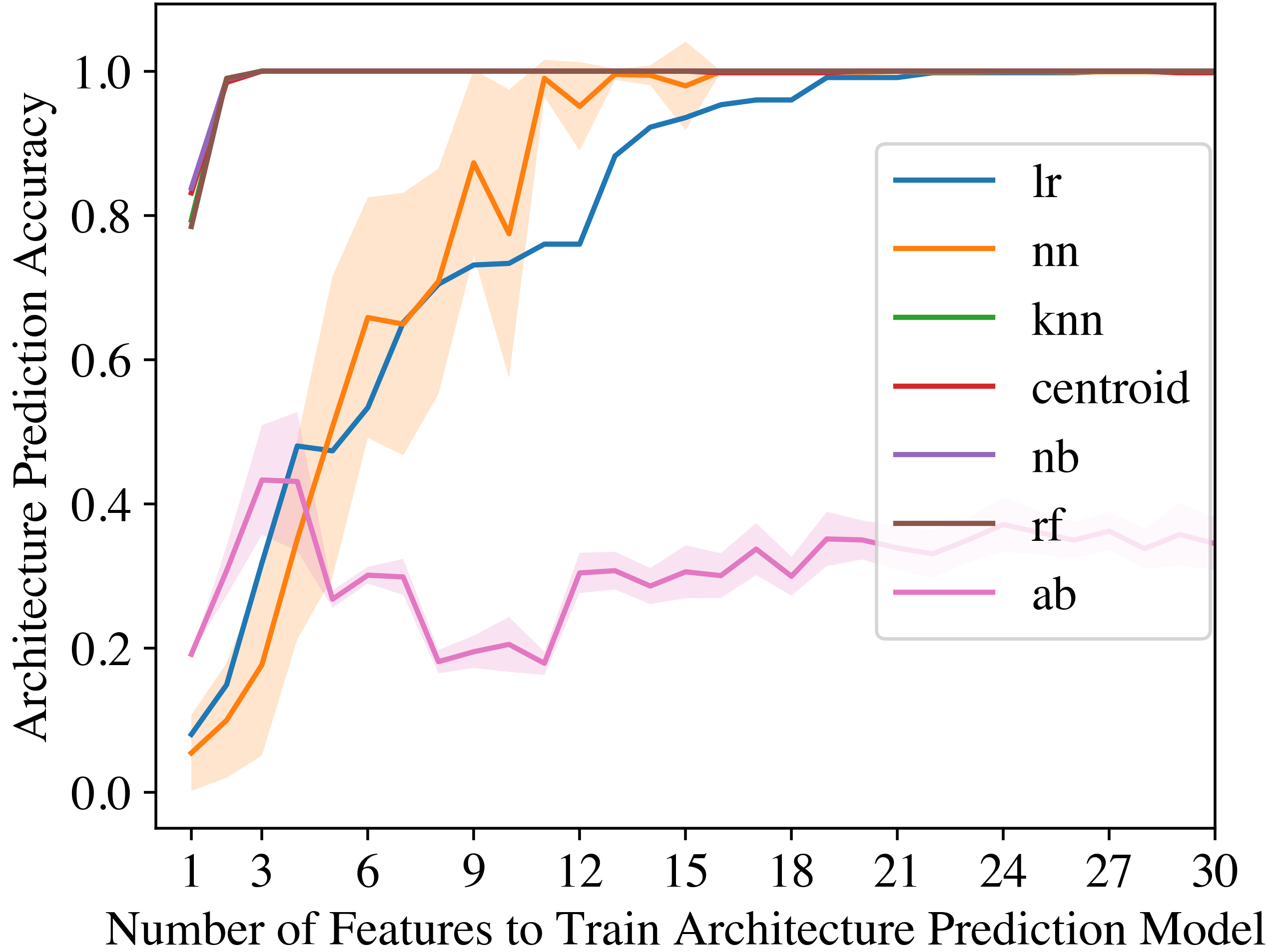
Figure 3: Top1 accuracy of architecture prediction models $\mathcal{A}$ on profiles in dataset $D_{2}$ by number of non-memory GPU kernel features used to train $\mathcal{A}$. Architecture prediction models were trained on dataset $D_{1}$. Lines and shaded regions denote the mean and standard deviation over 10 trials. Results overlap for K Nearest Neighbors, Centroid, Naive Bayes, and Random Forest architecture prediction models.

Due to the overfitting problem and the disparity in feature importance, we hypothesize that a small number of features would be sufficient for high architecture prediction accuracy. We consider only the 230 GPU kernel features without memory procedures because this is the narrowest subset of the features on which the accuracy was high on both the train $D_{1}$ and test $D_{2}$ datasets. We run SKLearn’s Recursive Feature Elimination (RFE) [13] feature selection algorithm to rank these features, then train the architecture prediction models $\mathcal{A}$ on $D_{1}$ using only the $m$ most important of these features. The viable models on which RFE can be applied are Logistic Regression, Random Forest, and AdaBoost. We choose Random Forest because it had the highest accuracy on the 230 features. We then evaluate the architecture prediction accuracy on $D_{2}$. The results are shown in Figure 3.

Our results confirm our hypothesis that a small number of features are sufficient for architecture prediction accuracy. While Table 3 demonstrates that architecture prediction models (except AdaBoost) can achieve high accuracy using over 200 GPU kernel features, Figure 3 shows that the same accuracy can be achieved using only 3 features for K Nearest Neighbors, Nearest Centroid, Naive Bayes, and Random Forest, 17 for Neural Network, and 22 for Logistic Regression. The top three features, shown in Figure 1 include the total time spent over the application running a vectorized tensor compare kernel, the average time spent per call to batch normalization kernel over the application, and the total time spent over the application running a convolution kernel.

Now that we have identified the most relevant profile features, we investigate the realistic scenario where no relationship is required between the parameters $\theta$ from the victim model $f_{v}^{\theta}$ and $\theta_{i}$ from candidate models $f_{c_{i}}^{\theta_{i}}$. In this case, the adversary may use pretrained candidate models $f_{c_{i}}^{\theta_{i}}$ which are widely available online, rather than train candidate models themselves. This reduces the complexity of the attack. Additionally, the adversary does not need to collect a dataset to train candidate models, nor does the adversary need to know the data distribution on which the victim model was trained. This assumes a less powerful adversary.

We generate a third dataset of profiles $D_{3}$ by profiling all 36 PyTorch vision DNNs trained on CIFAR10 [21]. We then train architecture prediction models $\mathcal{A}$ on $D_{1}$ (profiles collected on all 36 Pytorch vision DNNs trained on ImageNet) using the top 3 and 25 GPU kernel features based on the findings from Figure 3, and on all 230 GPU kernel features ranked by RFE. As in the previous experiments, the profiles in $D_{1}$ represent the profiles collected in the preprocessing stage of EZClone. We test the architecture prediction models on $D_{3}$ by treating the profiles in $D_{3}$ as if they were the victim model profiles obtained in Step 3 of EZClone. The parameters $\theta_{i}$ from the candidate models $f_{c_{i}}^{\theta_{i}}$ (dataset $D_{1}$) are derived from training on ImageNet and the candidate models have 1000 output classes, while the parameters $\theta$ from the victim models $f_{v}^{\theta}$ (dataset $D_{3}$) are derived from training on CIFAR10 and the victim models have 10 output classes.

Architecture Prediction Model $\mathcal{A}$	Top 3 Features	Top 25 Features	All 230 Features
Logistic Regression	40.0/41.6	99.9/100	99.1/55.5
Neural Network	17.0/19.4	100/94.4	100/58.3
K Nearest Neighbors	100/100	100/100	100/83.3
Nearest Centroid	100/100	100/100	98.3/83.3
Naive Bayes	100/97.2	100/100	100/66.6
Random Forest	100/100	100/100	100/100
AdaBoost	16.7/16.7	36.1/36.1	30.5/27.7

Table 4: Top1 Train ($D_{1}$) / Test ($D_{3}$) architecture prediction accuracy for architecture prediction models $\mathcal{A}$ by the top 3, 25, and 230 GPU kernel features (without memory data) used to train $\mathcal{A}$. $D_{1}$ consists of profiles generated by models trained on ImageNet, and $D_{2}$ consists of profiles generated by models trained on CIFAR10.

Results are shown in Table 4. In summary, these results demonstrate that EZClone can predict all 36 PyTorch vision model architectures even when the adversary uses candidate models with different parameters than the victim models and when the number of output classes differs. We see that the same top 3 features which enabled high accuracy for K Nearest Neighbors, Nearest Centroid, Naive Bayes, and Random Forest enable comparable accuracy on $D_{3}$, suggesting that these GPU kernel features are highly correlated with DNN architectures. The same holds true for the top 25 features with Logistic Regression and Neural Network. Interestingly, we see that training architecture prediction models on the entire set of 230 GPU kernel features without memory operations yields a similar overfitting problem as seen previously, although the top four performing models which were capable of learning with only 3 features (K Nearest Neighbors, Nearest Centroid, Naive Bayes, Random Forest) maintained at least 65% accuracy on all 230 features. This is most likely because the difference in number of output classes changes the size of the last fully connected layer in the network, which will affect some of the 230 non-memory GPU kernel features, but not the top 3 features.

Next, we examine the degree to which we can reduce computational demand of EZClone while maintaining accuracy. In particular, we would like to reduce the time necessary to complete Step 1 of EZClone: collecting profiles on all of the candidate architectures. Profiling a DNN takes around 45 seconds, so generating dataset $D_{1}$ (36 candidate architectures, 38 profiles per architecture) takes about 17 hours. The adversary would prefer to minimize this, although, on the bright side, the preprocessing step is a fixed cost that only needs to be completed once, and from thereon the online stage of EZClone is a matter of profiling a victim model and feeding the profile to the architecture prediction model, which takes less than one minute.

Given the high performance of architecture prediction models, we hypothesize that the training dataset for architecture prediction models need not be very large. To test this, we train architecture prediction models $\mathcal{A}$ on subsets of $D_{1}$, varying the number of profiles per candidate architecture. We use only the top 25 GPU kernel features without memory operations while training. We then test the architecture prediction models on $D_{3}$ to determine whether the smaller training set affects performance.

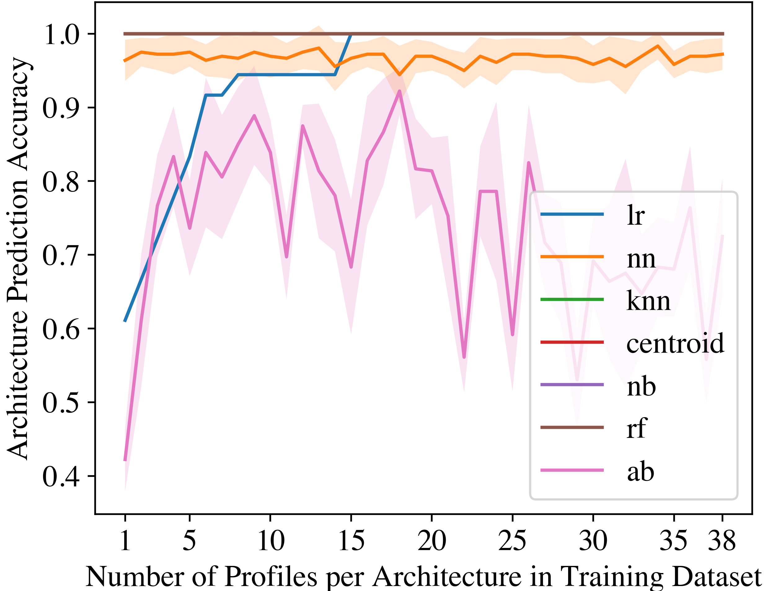
Figure 4: Top1 accuracy of architecture prediction models $\mathcal{A}$ on profiles in dataset $D_{3}$ by number of profiles per candidate architecture from $D_{1}$ used to train $\mathcal{A}$. Lines and shaded regions denote the mean and standard deviation over 10 trials. Results overlap for K Nearest Neighbors, Centroid, Naive Bayes, and Random Forest architecture prediction models.

The results are shown in Figure 4, which confirms our hypothesis that training on subsets of $D_{1}$ may achieve the same accuracy as training on the entirety of $D_{1}$. Surprisingly, for all architecture prediction models except Logistic Regression and AdaBoost, only one profile per candidate architecture was necessary to achieve the same accuracy as the full size of dataset $D_{1}$. These results indicate that the variance of the top 25 GPU kernels is low enough to allow generalization with only one sample per DNN architecture. With this in mind, the adversary only needs to collect 36 profiles, one per candidate architecture, to cover all PyTorch vision architectures, and preprocessing stage of EZClone can be completed in under 30 minutes. These results also suggest that to add one more DNN architecture to the candidate set in EZClone, only one more profile needs to be collected, adding about 45 seconds to the preprocessing phase.

Architecture Prediction Model $\mathcal{A}$	Logistic Regression	Neural Network	K Nearest Neighbors	Nearest Centroid	Naive Bayes	Random Forest	AdaBoost
Top1/Top5	94.4/100	80.6/91.7	97.2/97.2	97.2/97.2	100/100	100/100	30.6/41.7
Top1 Family Accuracy	100	88.9	100	100	100	100	47.2

Table 5: Top1/Top5 test accuracy of architecture prediction models trained on profiles from unpruned models and tested on profiles of pruned models. Family Top1 denotes if the predicted model architecture comes from the same family as the true model architecture.

Extending EZClone to Pruned Models: Next, we investigate whether DNN pruning affects the efficacy of EZClone. Since DNNs are computationally expensive, AI providers might use DNN optimizations such as pruning before deploying a victim model. To test this, we create a dataset $D_{p}$ of profiles on all 36 PyTorch vision models trained on CIFAR10 and pruned to 50% capacity. We then train architecture prediction models $\mathcal{A}$ on the top 25 non-memory GPU features of dataset $D_{1}$ and test the accuracy of $\mathcal{A}$ on $D_{p}$.

Table 5 displays these results, plus the family accuracy, which denotes if the predicted model architecture comes from the same family as the true model architecture. For example, ResNet18 and ResNet34 come from the same family while ResNet18 and GoogleNet do not. We find that, in general, the EZClone attack extends to pruned models while incurring a slight decrease in accuracy. Some models, such as Naive Bayes and Random Forest, incurred no loss in accuracy. These results show that the architecture prediction models $\mathcal{A}$ can generalize to profiles of pruned models even if they are not trained on profiles of pruned models. Based on the findings from Table 4, we expected these results because PyTorch is not optimized to skip operations on pruned parameters, meaning that pruning is just another form of differing the parameters $\theta_{i}$ and $\theta$ between the profiled candidate models $f_{c_{i}}^{\theta_{i}}$ and the victim models $f_{v}^{\theta}$.

EZClone Efficacy Across GPUs: We examine the ability of the EZClone attack to transfer across GPUs. Specifically, we consider the case where the adversary performs the EZClone preprocessing Step 1 of collecting profiles on candidate architectures on GPU $A$, and then performs the online Step 3 of collecting a profile on a victim model on GPU $B$. The adversary would prefer to do this if they don’t have easy access to GPU $B$ and/or risk being detected the longer they use the system with the victim model and GPU $B$.

Datasets $D_{1}$, $D_{2}$, and $D_{3}$ were generated using an Nvidia Quadro RTX 8000 GPU [29]. We collect two more profile datasets $D_{1}^{\prime}$ and $D_{3}^{\prime}$ using an Nvidia Tesla T4 GPU [30]. $D_{1}^{\prime}$ resembles $D_{1}$ in that the candidate models were trained on ImageNet, although we collect 13 profiles per candidate architecture instead of the 38 in $D_{1}$. $D_{3}^{\prime}$ is the same as $D_{3}$ (profiles on all PyTorch vision models trained on CIFAR10). As in previous experiements, we treat $D_{1}$ and $D_{1}^{\prime}$ as the training data that would be collected in the preprocessing phase of EZClone and only use the top 25 non-memory GPU kernel features. We treat each profile in $D_{3}$ and $D_{3}^{\prime}$ as a profile of a victim model (akin to a test set). We then test the EZClone attack when the training data comes from the Nvidia Quadro RTX 8000 and the test data comes from the Nvidia Tesla T4, and vice versa.

Architecture Prediction Model $\mathcal{A}$	Train Quadro RTX 8000, Test Tesla T4		Train Tesla T4, Test Quadro RTX 8000
	Top1/Top5	Family Top1	Top1/Top5	Family Top1
Logistic Reg	33.3/75.0	77.8	27.8/55.6	47.2
Neural Net	11.1/27.8	33.3	11.1/25.0	30.6
KNN	36.1/41.7	75.0	27.8/27.8	50.0
Centroid	36.1/41.7	75.0	27.8/27.8	50.0
Naive Bayes	72.2/72.2	97.2	75.0/75.0	97.2
Rand Forest	41.7/75.0	80.6	44.4/77.8	58.3
AdaBoost	5.56/27.8	25.0	33.3/63.9	66.7

Table 6: Top1/Top5 test accuracy of architecture prediction models trained on profiles from one GPU and tested on profiles from another GPU. Training data consists of profiles of candidate models trained on ImageNet, while test data consists of profiles of candidate models trained on CIFAR10.

While building datasets $D_{1}^{\prime}$ and $D_{3}^{\prime}$, we find that all 25 non-memory GPU kernels, which were chosen based on $D_{1}$, were also present in $D_{1}^{\prime}$ and $D_{3}^{\prime}$. This indicates that DNN architectures use the some of the same GPU kernels even when the GPU changes. This also holds between different CUDA versions (the Nvidia Quadro RTX 8000 used 10.2.89 and the Nvidia Tesla T4 used 11.2.152).

Table 6 displays the top1, top5, and family accuracy of training on one GPU and testing on another. We find that in general the intra-GPU accuracy results such as those reported in Table 4 do not hold across GPUs. Additionally, training on the Quadro RTX 8000 GPU and testing on the Tesla T4 GPU performed better than the other way around.

Despite the decrease in accuracy, the EZClone attack still provides value across GPUs. The Naive Bayes architecture prediction model attained over 72% cross-GPU accuracy. Furthermore, many architecture prediction models had reasonable family accuracy. Prior work [26, 34, 32] show that a surrogate model from the same family as the victim model improves adversarial attacks, which benefits a reconaissance-motivated adversary. Additionally, if there were only one candidate architecture per family in the candidate set, then the family accuracy would become the top1 accuracy. This means that if the EZClone attack is weakened to be able to predict less DNN architectures, the transferability of the attack across GPUs strengthens.

6 PyTorch Parser

To implement the PyTorch Trace Parser, we create a mapping between the calls to a DNN layer type in the PyTorch API and the GPU kernels executed as a result of that call, similarly to the preprocessing step in the Hermes attack [55]. We also map between the layer hyperparameters in the high level PyTorch code and the layer hyperparameters in the PyTorch profile.

Since all of the GPU kernels and layer hyperparameters are recovered from the PyTorch Profiler, we use the mapping to parse the architecture from the PyTorch profile. We find that the parser is able to reconstruct all of the PyTorch vision models.

7 Future Work

Future investigation into the efficacy of EZClone may examine several parameters. The size of the candidate set may be increased to include new models added to PyTorch. The attack may be tested on a variety of GPUs in different environments, such as mobile or edge devices, and using a variety of profilers. EZClone may be tested on different machine learning frameworks, including TensorFlow, TensorFlow Lite, and ONNX, or the new PyTorch v2.0 [38], which reduces the number of primitive operators used to run a DNN. Optimizing frameworks by reducing the size of the operation set may increase the efficacy of EZClone since the same GPU kernels will be invoked, producing a smaller and representative feature set with a higher signal to noise ratio.

Next, a mitigation to EZClone might include adding dummy computation to disrupt the signal-to-noise ratio in the side-channel. This study would involve determining the relationship between the amount of dummy computation, the efficacy of the attack, and the resultant performance overhead. This has been suggested in prior work [15, 26, 55]. Precision limiting the GPU profile information [28, 47], may also mitigate EZClone, but decreases the value of the intended fair use of GPU profilers. A baseline mitigation for EZClone should be to ensure sudo priviledges are required to use GPU profilers on any system running a victim DNN.

8 Conclusion

We propose EZClone, a simple, fast, and accurate method to recover the architecture of a DNN using GPU profiles as a side-channel. A distinguishing feature of the EZClone attack is that it does not use time-series data, so defenses against time-series based attacks may not also mitigate EZClone. We demonstrate that EZClone can recover all 36 PyTorch vision models with 100% accuracy, using only 3 features empirically found from the side channel information. We also show that EZClone maintains accuracy when deployed on models which have different parameters than the training set of side channel information, and on pruned victim models. Futhermore, EZClone is easily extensible; to predict a new architecture, EZClone requires only one profile of a model with that architecture, taking less than one minute to complete.

Additionally, we develop a parser for PyTorch generated profiles which can recover DNN architectures. This uncovers a new attack surface, where a malicious library may leak the DNN architecture with no loss in library functionality and only one line of code changed.

EZClone and the PyTorch parser improve and extend architecture extraction methods which use side-channel information to recover the architecture of a DNN as the first step in a model extraction attack. After extracting the architecture, an adversary will extract the parameters of the DNN, breaking the confidentiality of the model. The adversary may then run further attacks which comprimise the integrity of the model or the privacy of the data on which it was trained. These vulnerabilities motivate the need for comprehensive defense techniques against model extraction.

9 Acknowledgement

This work has been supported in part by a grant from the National Science Foundation.

10 Availability

Code is available at https://github.com/{redacted}, including Python modules for all the components of EZClone: collecting aggregate GPU profiles, training an architecture prediction model, and predicting DNN architectures. There is also a module for extracting victim DNN architectures through the PyTorch parser.

Appendix A Appendix

AlexNet	VGG13	GoogleNet
ResNet18	VGG13_bn	MobileNet_v2
ResNet34	VGG16	MobileNet_v3_large
ResNet50	VGG16_bn	MobileNet_v3_small
ResNet101	VGG19	MnasNet0_5
ResNet152	VGG19_bn	MnasNet0_75
ResNext50_32x4d	SqueezeNet1_0	MnasNet1_0
ResNext101_32x8d	SqueezeNet1_1	MnasNet1_3
Wide_ResNet50_2	DenseNet121	ShuffleNet_v2_x0_5
Wide_ResNet101_2	DenseNet169	ShuffleNet_v2_x1_0
VGG11	DenseNet201	ShuffleNet_v2_x1_5
VGG11_bn	DenseNet161	ShuffleNet_v2_x2_0

Table 7: The 36 PyTorch vision architectures which were used in evaluating the EZClone attack. These are all of the architectures present in Torchvision v0.10.0 [37].

References

- [1] Akhtar, N., Mian, A., Kardan, N., and Shah, M. Threat of adversarial attacks on deep learning in computer vision: Survey II. CoRR abs/2108.00401 (2021). https://arxiv.org/abs/2108.00401.
- [2] Akhtar, N., and Mian, A. S. Threat of adversarial attacks on deep learning in computer vision: A survey. IEEE Access 6 (2018), 14410–14430. https://doi.org/10.1109/ACCESS.2018.2807385.
- [3] Batina, L., Bhasin, S., Jap, D., and Picek, S. CSI NN: reverse engineering of neural network architectures through electromagnetic side channel. In 28th USENIX Security Symposium, USENIX (2019), N. Heninger and P. Traynor, Eds., USENIX Association, pp. 515–532. https://www.usenix.org/conference/usenixsecurity19/presentation/batina.
- [4] Carlini, N., Jagielski, M., and Mironov, I. Cryptanalytic extraction of neural network models. In Advances in Cryptology - CRYPTO (2020), D. Micciancio and T. Ristenpart, Eds., vol. 12172 of Lecture Notes in Computer Science, Springer, pp. 189–218. https://doi.org/10.1007/978-3-030-56877-1_7.
- [5] Chabanne, H., Danger, J., Guiga, L., and Kühne, U. Side channel attacks for architecture extraction of neural networks. CAAI Trans. Intell. Technol. 6, 1 (2021), 3–16. https://doi.org/10.1049/cit2.12026.
- [6] Chakraborty, A., Alam, M., Dey, V., Chattopadhyay, A., and Mukhopadhyay, D. A survey on adversarial attacks and defences. CAAI Trans. Intell. Technol. 6, 1 (2021), 25–45. https://doi.org/10.1049/cit2.12028.
- [7] Chitty-Venkata, K. T., and Somani, A. K. Neural architecture search survey: A hardware perspective. ACM Comput. Surv. 55, 4 (2023), 78:1–78:36. https://doi.org/10.1145/3524500.
- [8] Chmielewski, L., and Weissbart, L. On reverse engineering neural network implementation on GPU. In Applied Cryptography and Network Security Workshops - ACNS (2021), vol. 12809, Springer, pp. 96–113. https://doi.org/10.1007/978-3-030-81645-2_7.
- [9] da Silva, J. R. C., Berriel, R. F., Badue, C., Souza, A. F. D., and Oliveira-Santos, T. Copycat CNN: are random non-labeled data enough to steal knowledge from black-box models? CoRR abs/2101.08717 (2021). https://arxiv.org/abs/2101.08717.
- [10] Deng, J., Dong, W., Socher, R., Li, L., Li, K., and Fei-Fei, L. Imagenet: A large-scale hierarchical image database. In 2009 IEEE Computer Society Conference on Computer Vision and Pattern Recognition CVPR (2009), IEEE Computer Society, pp. 248–255. https://doi.org/10.1109/CVPR.2009.5206848.
- [11] Docs., T. Tensorboard documentation. https://www.tensorflow.org/tensorboard.
- [12] Gong, X., Chen, Y., Yang, W., Mei, G., and Wang, Q. Inversenet: Augmenting model extraction attacks with training data inversion. In Proceedings of the Thirtieth International Joint Conference on Artificial Intelligence, IJCAI (2021), Z. Zhou, Ed., ijcai.org, pp. 2439–2447. https://doi.org/10.24963/ijcai.2021/336.
- [13] Guyon, I., Weston, J., Barnhill, S., and Vapnik, V. Gene selection for cancer classification using support vector machines. Mach. Learn. 46, 1-3 (2002), 389–422. https://doi.org/10.1023/A:1012487302797.
- [14] Han, S., Pool, J., Tran, J., and Dally, W. J. Learning both weights and connections for efficient neural networks. CoRR abs/1506.02626 (2015). http://arxiv.org/abs/1506.02626.
- [15] Hong, S., Davinroy, M., Kaya, Y., Locke, S. N., Rackow, I., Kulda, K., Dachman-Soled, D., and Dumitras, T. Security analysis of deep neural networks operating in the presence of cache side-channel attacks. CoRR abs/1810.03487 (2018). http://arxiv.org/abs/1810.03487.
- [16] Hu, X., Liang, L., Li, S., Deng, L., Zuo, P., Ji, Y., Xie, X., Ding, Y., Liu, C., Sherwood, T., and Xie, Y. Deepsniffer: A DNN model extraction framework based on learning architectural hints. In ASPLOS ’20: Architectural Support for Programming Languages and Operating Systems, Lausanne (2020), J. R. Larus, L. Ceze, and K. Strauss, Eds., ACM, pp. 385–399. https://doi.org/10.1145/3373376.3378460.
- [17] Hua, W., Zhang, Z., and Suh, G. E. Reverse engineering convolutional neural networks through side-channel information leaks. In Proceedings of the 55th Annual Design Automation Conference, DAC (2018), ACM, pp. 4:1–4:6. https://doi.org/10.1145/3195970.3196105.
- [18] IEEE. The radical scope of tesla’s data hoard. https://spectrum.ieee.org/tesla-autopilot-data-scope, Aug 2022.
- [19] Jagielski, M., Carlini, N., Berthelot, D., Kurakin, A., and Papernot, N. High accuracy and high fidelity extraction of neural networks. In 29th USENIX Security Symposium, USENIX (2020), S. Capkun and F. Roesner, Eds., USENIX Association, pp. 1345–1362. https://www.usenix.org/conference/usenixsecurity20/presentation/jagielski.
- [20] Jha, N. K., Mittal, S., Kumar, B., and Mattela, G. Deeppeep: Exploiting design ramifications to decipher the architecture of compact dnns. ACM 17, 1 (2020), 5:1–5:25. https://doi.org/10.1145/3414552.
- [21] Krizhevsky, A., Hinton, G., et al. Learning multiple layers of features from tiny images. https://www.cs.toronto.edu/~kriz/learning-features-2009-TR.pdf.
- [22] Krizhevsky, A., Sutskever, I., and Hinton, G. E. Imagenet classification with deep convolutional neural networks. In Advances in Neural Information Processing Systems 25: 26th Annual Conference on Neural Information Processing Systems (2012), P. L. Bartlett, F. C. N. Pereira, C. J. C. Burges, L. Bottou, and K. Q. Weinberger, Eds., pp. 1106–1114. https://proceedings.neurips.cc/paper/2012/hash/c399862d3b9d6b76c8436e924a68c45b-Abstract.html.
- [23] Liu, S., Wei, Y., Chi, J., Shezan, F. H., and Tian, Y. Side channel attacks in computation offloading systems with GPU virtualization. In 2019 IEEE Security and Privacy Workshops, SP (2019), IEEE, pp. 156–161. https://doi.org/10.1109/SPW.2019.00037.
- [24] Liu, Y., and Srivastava, A. GANRED: gan-based reverse engineering of dnns via cache side-channel. In CCSW’20, Proceedings of the 2020 ACM SIGSAC Conference on Cloud Computing Security Workshop (2020), Y. Zhang and R. Sion, Eds., ACM, pp. 41–52. https://doi.org/10.1145/3411495.3421356.
- [25] Liu, Y., Zuzak, M., Xing, D., McDaniel, I., Mittu, P., Ozbay, O., Akib, A., and Srivastava, A. A survey on side-channel-based reverse engineering attacks on deep neural networks. In 4th IEEE International Conference on Artificial Intelligence Circuits and Systems, AICAS (2022), IEEE, pp. 312–315. https://doi.org/10.1109/AICAS54282.2022.9869995.
- [26] Maia, H. T., Xiao, C., Li, D., Grinspun, E., and Zheng, C. Can one hear the shape of a neural network?: Snooping the GPU via magnetic side channel. In 31st USENIX Security Symposium, USENIX (2022), K. R. B. Butler and K. Thomas, Eds., USENIX Association, pp. 4383–4400. https://www.usenix.org/conference/usenixsecurity22/presentation/maia.
- [27] Mittal, S., Gupta, H., and Srivastava, S. A survey on hardware security of DNN models and accelerators. J. Syst. Archit. 117 (2021), 102163. https://doi.org/10.1016/j.sysarc.2021.102163.
- [28] Naghibijouybari, H., Neupane, A., Qian, Z., and Abu-Ghazaleh, N. B. Rendered insecure: GPU side channel attacks are practical. In Proceedings of the 2018 ACM SIGSAC Conference on Computer and Communications Security, CCS (2018), D. Lie, M. Mannan, M. Backes, and X. Wang, Eds., ACM, pp. 2139–2153. https://doi.org/10.1145/3243734.3243831.
- [29] Nvidia. Nvidia quadro rtx 8000 gpu datasheet. https://www.nvidia.com/content/dam/en-zz/Solutions/design-visualization/quadro-product-literature/quadro-rtx-8000-us-nvidia-946977-r1-web.pdf, Mar 2019.
- [30] Nvidia. Nvidia tesla t4 gpu datasheet. https://www.nvidia.com/content/dam/en-zz/Solutions/Data-Center/tesla-t4/t4-tensor-core-datasheet-951643.pdf, Mar 2019.
- [31] Nvidia. Profiler user’s guide. https://docs.nvidia.com/cuda/archive/10.2/profiler-users-guide/index.html, Nov 2019.
- [32] Oh, S. J., Schiele, B., and Fritz, M. Towards reverse-engineering black-box neural networks. In Explainable AI: Interpreting, Explaining and Visualizing Deep Learning, W. Samek, G. Montavon, A. Vedaldi, L. K. Hansen, and K. Müller, Eds., vol. 11700 of Lecture Notes in Computer Science. Springer, 2019, pp. 121–144. https://doi.org/10.1007/978-3-030-28954-6_7.
- [33] Orekondy, T., Schiele, B., and Fritz, M. Knockoff nets: Stealing functionality of black-box models. In IEEE Conference on Computer Vision and Pattern Recognition, CVPR (2019), Computer Vision Foundation / IEEE, pp. 4954–4963. http://openaccess.thecvf.com/content_CVPR_2019/html/Orekondy_Knockoff_Nets_Stealing_Functionality_of_Black-Box_Models_CVPR_2019_paper.html.
- [34] Papernot, N., McDaniel, P. D., Goodfellow, I. J., Jha, S., Celik, Z. B., and Swami, A. Practical black-box attacks against machine learning. In Proceedings of the 2017 ACM on Asia Conference on Computer and Communications Security (2017), R. Karri, O. Sinanoglu, A. Sadeghi, and X. Yi, Eds., ACM, pp. 506–519. https://doi.org/10.1145/3052973.3053009.
- [35] Papernot, N., McDaniel, P. D., Sinha, A., and Wellman, M. P. Sok: Security and privacy in machine learning. In 2018 IEEE European Symposium on Security and Privacy, EuroS&P (2018), IEEE, pp. 399–414. https://doi.org/10.1109/EuroSP.2018.00035.
- [36] Patwari, K., Hafiz, S. M., Wang, H., Homayoun, H., Shafiq, Z., and Chuah, C. DNN model architecture fingerprinting attack on CPU-GPU edge devices. In 7th IEEE European Symposium on Security and Privacy, EuroS&P (2022), IEEE, pp. 337–355. https://doi.org/10.1109/EuroSP53844.2022.00029.
- [37] PyTorch. Torchvision v0.10.0 documentation. https://pytorch.org/vision/0.10/, Jun 2021.
- [38] PyTorch. Pytorch 2.0. https://pytorch.org/get-started/pytorch-2.0/, Dec 2022.
- [39] PyTorch. Pytorch profiler documentation. https://pytorch.org/tutorials/recipes/recipes/profiler_recipe.html, Dec 2022.
- [40] Radford, A., Narasimhan, K., Salimans, T., and Sutskever, I. Improving language understanding by generative pre-training. https://www.bibsonomy.org/bibtex/273ced32c0d4588eb95b6986dc2c8147c/jonaskaiser.
- [41] Sculley, D., Holt, G., Golovin, D., Davydov, E., Phillips, T., Ebner, D., Chaudhary, V., Young, M., Crespo, J., and Dennison, D. Hidden technical debt in machine learning systems. In Advances in Neural Information Processing Systems 28: Annual Conference on Neural Information Processing Systems (2015), C. Cortes, N. D. Lawrence, D. D. Lee, M. Sugiyama, and R. Garnett, Eds., pp. 2503–2511. https://proceedings.neurips.cc/paper/2015/hash/86df7dcfd896fcaf2674f757a2463eba-Abstract.html.
- [42] Sharir, O., Peleg, B., and Shoham, Y. The cost of training NLP models: A concise overview. CoRR abs/2004.08900 (2020). https://arxiv.org/abs/2004.08900.
- [43] Simonyan, K., and Zisserman, A. Very deep convolutional networks for large-scale image recognition. In 3rd International Conference on Learning Representations, ICLR (2015), Y. Bengio and Y. LeCun, Eds. http://arxiv.org/abs/1409.1556.
- [44] Sutskever, I., Vinyals, O., and Le, Q. V. Sequence to sequence learning with neural networks. In Advances in Neural Information Processing Systems 27: Annual Conference on Neural Information Processing Systems (2014), Z. Ghahramani, M. Welling, C. Cortes, N. D. Lawrence, and K. Q. Weinberger, Eds., pp. 3104–3112. https://proceedings.neurips.cc/paper/2014/hash/a14ac55a4f27472c5d894ec1c3c743d2-Abstract.html.
- [45] Tramèr, F., Zhang, F., Juels, A., Reiter, M. K., and Ristenpart, T. Stealing machine learning models via prediction apis. In 25th USENIX Security Symposium, USENIX (2016), T. Holz and S. Savage, Eds., USENIX Association, pp. 601–618. https://www.usenix.org/conference/usenixsecurity16/technical-sessions/presentation/tramer.
- [46] Vaswani, A., Shazeer, N., Parmar, N., Uszkoreit, J., Jones, L., Gomez, A. N., Kaiser, L., and Polosukhin, I. Attention is all you need. In Advances in Neural Information Processing Systems 30: Annual Conference on Neural Information Processing Systems (2017), I. Guyon, U. von Luxburg, S. Bengio, H. M. Wallach, R. Fergus, S. V. N. Vishwanathan, and R. Garnett, Eds., pp. 5998–6008. https://proceedings.neurips.cc/paper/2017/hash/3f5ee243547dee91fbd053c1c4a845aa-Abstract.html.
- [47] Wei, J., Zhang, Y., Zhou, Z., Li, Z., and Faruque, M. A. A. Leaky DNN: stealing deep-learning model secret with GPU context-switching side-channel. In 50th Annual IEEE/IFIP International Conference on Dependable Systems and Networks, DSN (2020), IEEE, pp. 125–137. https://doi.org/10.1109/DSN48063.2020.00031.
- [48] Xiang, Y., Chen, Z., Chen, Z., Fang, Z., Hao, H., Chen, J., Liu, Y., Wu, Z., Xuan, Q., and Yang, X. Open DNN box by power side-channel attack. IEEE Trans. Circuits Syst. 67-II, 11 (2020), 2717–2721. https://doi.org/10.1109/TCSII.2020.2973007.
- [49] Xiong, W., Droppo, J., Huang, X., Seide, F., Seltzer, M., Stolcke, A., Yu, D., and Zweig, G. The microsoft 2016 conversational speech recognition system. In 2017 IEEE International Conference on Acoustics, Speech and Signal Processing, ICASSP (2017), IEEE, pp. 5255–5259. https://doi.org/10.1109/ICASSP.2017.7953159.
- [50] Xu, Q., Arafin, M. T., and Qu, G. Security of neural networks from hardware perspective: A survey and beyond. In ASPDAC ’21: 26th Asia and South Pacific Design Automation Conference (2021), ACM, pp. 449–454. https://doi.org/10.1145/3394885.3431639.
- [51] Yan, M., Fletcher, C. W., and Torrellas, J. Cache telepathy: Leveraging shared resource attacks to learn DNN architectures. In 29th USENIX Security Symposium, USENIX (2020), S. Capkun and F. Roesner, Eds., USENIX Association, pp. 2003–2020. https://www.usenix.org/conference/usenixsecurity20/presentation/yan.
- [52] Yu, H., Ma, H., Yang, K., Zhao, Y., and Jin, Y. Deepem: Deep neural networks model recovery through EM side-channel information leakage. In 2020 IEEE International Symposium on Hardware Oriented Security and Trust, HOST (2020), IEEE, pp. 209–218. https://doi.org/10.1109/HOST45689.2020.9300274.
- [53] Yu, H., Yang, K., Zhang, T., Tsai, Y., Ho, T., and Jin, Y. Cloudleak: Large-scale deep learning models stealing through adversarial examples. In 27th Annual Network and Distributed System Security Symposium, NDSS (2020), The Internet Society. https://www.ndss-symposium.org/ndss-paper/cloudleak-large-scale-deep-learning-models-stealing-through-adversarial-examples/.
- [54] Yuan, X., Ding, L., Zhang, L., Li, X., and Wu, D. O. ES attack: Model stealing against deep neural networks without data hurdles. IEEE Trans. Emerg. Top. Comput. Intell. 6, 5 (2022), 1258–1270. https://doi.org/10.1109/TETCI.2022.3147508.
- [55] Zhu, Y., Cheng, Y., Zhou, H., and Lu, Y. Hermes attack: Steal DNN models with lossless inference accuracy. In 30th USENIX Security Symposium, USENIX (2021), M. Bailey and R. Greenstadt, Eds., USENIX Association, pp. 1973–1988. https://www.usenix.org/conference/usenixsecurity21/presentation/zhu.
- [56] Zou, P., Li, A., Barker, K. J., and Ge, R. Fingerprinting anomalous computation with RNN for gpu-accelerated HPC machines. In IEEE International Symposium on Workload Characterization, IISWC (2019), IEEE, pp. 253–256. https://doi.org/10.1109/IISWC47752.2019.9042165.