Neural Fields meet Explicit Geometric Representations
for Inverse Rendering of Urban Scenes

Abstract

Reconstruction and intrinsic decomposition of scenes from captured imagery would enable many applications such as relighting and virtual object insertion. Recent NeRF based methods achieve impressive fidelity of 3D reconstruction, but bake the lighting and shadows into the radiance field, while mesh-based methods that facilitate intrinsic decomposition through differentiable rendering have not yet scaled to the complexity and scale of outdoor scenes. We present a novel inverse rendering framework for large urban scenes capable of jointly reconstructing the scene geometry, spatially-varying materials, and HDR lighting from a set of posed RGB images with optional depth. Specifically, we use a neural field to account for the primary rays, and use an explicit mesh (reconstructed from the underlying neural field) for modeling secondary rays that produce higher-order lighting effects such as cast shadows. By faithfully disentangling complex geometry and materials from lighting effects, our method enables photorealistic relighting with specular and shadow effects on several outdoor datasets. Moreover, it supports physics-based scene manipulations such as virtual object insertion with ray-traced shadow casting.

1 Introduction

Reconstructing high fidelity 3D scenes from captured imagery is an important utility of scaleable 3D content creation. However, for the reconstructed environments to serve as “digital twins” for downstream applications such as augmented reality and gaming, we require that these environments are compatible with modern graphics pipeline and can be rendered with user-specified lighting. This means that we not only need to reconstruct 3D geometry and texture but also recover the intrinsic properties of the scene such as material properties and lighting information. This is an ill-posed, challenging problem oftentimes referred to as inverse rendering [1].

Neural radiance fields (NeRFs) [34] have recently emerged as a powerful neural reconstruction approach that enables photo-realistic novel-view synthesis. NeRFs can be reconstructed from a set of posed camera images in a matter of minutes [35, 14, 43] and have been shown to scale to room-level scenes and beyond [45, 48, 55], making them an attractive representation for augmented/virtual reality and generation of digital twins. However, in NeRF, the intrinsic properties of the scene are not separated from the effect of incident light. As a result, novel views can only be synthesised under fixed lighting conditions present in the input images, i.e. a NeRF cannot be relighted [42].

While NeRF can be extended into a full inverse rendering formulation [3], this requires computing the volume rendering integral when tracing multiple ray bounces. This quickly becomes intractable due to the underlying volumetric representation. Specifically, in order to estimate the secondary rays, the volumetric density field of NeRF would have to be queried along the path from each surface point to all the light sources, scaling with $\mathcal{O}(nm)$ per point, where $n$ denotes the number of samples along each ray and $m$ is the number of light sources or Monte Carlo (MC) samples in the case of global illumination. To restrict the incurred computational cost, prior works have mostly focused on the single object setting and often assume a single (known) illumination source [42]. Additionally, they forgo the volumetric rendering of secondary rays and instead approximate the direct/indirect lighting through a visibility MLP [42, 64].

In contrast to NeRF, the explicit mesh-based representation allows for very efficient rendering. With a known mesh topology, the estimation of both primary and secondary rays is carried out using ray-mesh intersection ($\mathcal{O}(m)$) queries that can be efficiently computed using highly-optimized libraries such as OptiX [39]. However, inverse rendering methods based on explicit mesh representations either assume a fixed mesh topology [13], or recover the surface mesh via an SDF defined on a volumetric grid [36] and are thus bounded by the grid resolution. Insofar, these methods have been shown to produce high-quality results only for the smaller, object-centric scenes.

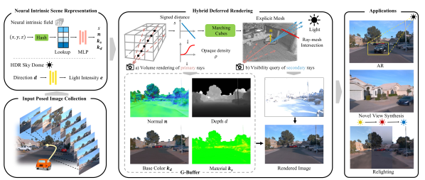
In this work, we combine the advantages of the neural field (NeRF) and explicit (mesh) representations and propose FEGR, a new hybrid-rendering pipeline for inverse rendering of large urban scenes. Specifically, we represent the intrinsic properties of the scene using a neural field and estimate the primary rays (G-buffer) with volumetric rendering. To model the secondary rays that produce higher-order lighting effects such as specular highlights and cast shadows, we convert the neural field to an explicit representation and preform physics-based rendering. The underlying neural field enables us to represent high-resolution details, while ray tracing secondary rays using the explicit mesh reduces the computational complexity. The proposed hybrid-rendering is fully differentiable an can be embedded into an optimization scheme that allows us to estimate 3D spatially-varying material properties, geometry, and HDR lighting of the scene from a set of posed camera images. By modeling the HDR properties of the scene, our representation is also well suited for AR applications such as virtual object insertion that require spatially-varying lighting to cast shadows in a physically correct way.

We summarize our contributions as follows:

• We propose a novel neural field representation that decomposes scene into geometry, spatially varying materials, and HDR lighting.

• To achieve efficient ray-tracing within a neural scene representation, we introduce a hybrid renderer that renders primary rays through volumetric rendering, and models the secondary rays using physics-based rendering. This enables high-quality inverse rendering of large urban scenes.

• We model the HDR lighting and material properties of the scene, making our representation well suited for downstream applications such as relighting and virtual object insertion with cast shadows.

FEGR significantly outperforms state-of-the-art in terms of novel-view synthesis under varying lighting conditions on the NeRF-OSR dataset [40]. We also show qualitative results on a single-illumination capture of an urban environment, collected by an autonomous vehicle. Moreover, we show the intrinsic rendering results, and showcase virtual object insertion as an application. Finally, we conduct a user study, in which the results of our method are significantly preferred to those of the baselines.

2 Related Work

Inverse Rendering

is a fundamental task in computer vision. The seminal work by Barrow and Tenenbaum [1] aimed to understand the intrinsic scene properties including reflectance, lighting, and geometry from captured imagery. Considering the ill-posed nature [24] of this challenging task, early works resided to tackle the subtask known as intrinsic image decomposition, that aims to decompose an image into diffuse albedo and shading. These methods are mostly optimization-based and rely on hand-crafted priors [24, 17, 10, 65]. In the deep learning era, learning-based methods [2, 22, 28, 41, 57, 27, 30, 9, 53, 52, 54] replaced the classic optimisation pipeline and learn the intrinsic decomposition in a data-driven manner, but typically require ground truth supervision. However, acquiring ground truth intrinsic decomposition in the real world is extremely challenging. Learning-based methods thus often train on synthetic datasets [28, 41, 27, 30, 53], and may suffer from a domain gap between synthetic and real captures. In addition, these methods are limited to 2.5D prediction, i.e. 2D intrinsic images and a normal map, thus are unable to reconstruct the full 3D scene. Recent advances in differentiable rendering [38] and neural volume rendering [34] revive the optimization paradigm by enabling direct optimization of the 3D scene representation [4, 6, 61, 8, 63, 60, 23, 36, 18, 7, 5]. However, these works mostly focus on a single object setting and ignore higher-order lighting effects such as cast shadows.

Figure 2: Overview of FEGR. Given a set of posed camera images, FEGR estimates the geometry, spatially varying materials, and HDR lighting of the underlying scene. We model the intrinsic properties of the scene using a neural intrinsic field and use an HDR Sky Dome to represent the lighting. Our Hybrid Deferred Renderer models the primary rays with volumetric rendering of the neural field, while the secondary rays are ray-traced using an explicit mesh reconstructed from the SD field. By modeling the HDR properties of the scene FEGR can support several scene manipulations including novel-view synthesis, scene relighting, and AR.

Neural Scene Representation

for inverse rendering mostly falls into two categories: explicit textured mesh [12, 37, 13, 59, 36, 18] and neural fields [4, 6, 61, 63, 60]. Explicit mesh representations [36, 18] are compatible with graphics pipeline and naturally benefit from classic graphics techniques. These methods show impressive performance under single-object setting but suffers from bounded resolution when scaling up to a larger scene extent. With the impressive image synthesis quality demonstrated by neural fields [34], recent works on inverse rendering also adopt neural fields as representation for scene intrinsic properties [4, 6, 61, 63, 60, 50, 56]. Despite the impressive results for primary ray appearance, it remains an open challenge for neural fields to represent higher order lighting effects such as cast shadows via ray-tracing. To reduce the complexity of ray-tracing in neural fields, prior works explore using MLP to encode visibility field [42, 26] or Spherical Gaussian visibility [64], but typically limited to object-level or low-frequency effects. The closest setup to our work is NeRF-OSR [40] that works on outdoor scene-level inverse rendering. It uses a network to represent shadows and relys on multiple illumination to disentangle shadows from albedo, but usually cannot recover sharp shadow boundaries. Related to our work are also methods that factorize the appearance changes through latent codes [33, 31]. These methods can modify scene appearance by interpolation of the latent codes, but do not offer explicit control of lighting conditions.

Lighting Estimation

is a subtask of inverse rendering which aims to understand the lighting distribution across the scene, typically with the goal of photorealistic virtual object insertion. Existing work on lighting estimation is usually learning-based, adopting feed-forward neural networks given the input of a single image [29, 25, 16, 20, 19, 66, 52, 46]. For outdoor scenes, prior work investigates network designs to predict lighting representations such as a HDR sky model [20, 58, 19], spatially-varying environment map [66, 46] and a lighting volume [52]. The key challenge for outdoor lighting estimation is to correctly estimate the peak direction and intensity of the sky, which is usually the location of the sun. This is a challenging ill-posed task where a single image input may be insufficient to produce accurate results. Recent optimization-based inverse rendering works jointly optimize lighting from multi-view images [6, 61, 36, 18], however their primary purpose of lighting is to serve the joint optimization framework for recovering material properties. Lighting representations are usually point light [42] and low frequency spherical lobes [6, 61, 40], which are not suited for AR applications. In our work, we investigate optimization-based lighting estimation to directly optimize HDR lighting from visual cues in the input imagery, such as shadows. Our neural lighting representation is used as the light source for inserting virtual objects.

3 Method

Given a set of posed camera images $\{\mathbf{I}_{i},\mathbf{c}_{i}\}_{i=1}^{N_{\text{RGB}}}$, where $\mathbf{I}\in\mathbb{R}^{h\times w\times 3}$ is an image and $\mathbf{c}\in\text{SE}(3)$ is its corresponding camera pose, we aim to estimate the geometry, spatially varying materials, and HDR lighting of the underlying scene. We represent the intrinsic scene properties using a neural field (Sec. 3.1) and render the views with a differentiable hybrid renderer (Sec. 3.2). To estimate the parameters of the neural field, we minimize the reconstruction error on the observed views and employ several regularization terms to constrain the highly ill-posed nature of the problem (Sec. 3.3). Implementation details are provided in the Appendix.

Note that our method addresses both single- and multi-illumination intrinsic decomposition. Existing literature [40] considers the multi-illumination setting that efficiently constraints the solution space of intrinsic properties and thus leads to a more faithful decomposition, while our formulation is general, and we demonstrate its effectiveness even when in the case of a single illumination capture. In the following, we keep the writing general, and address the distinction where required.

3.1 Neural Intrinsic Scene Representation

Neural intrinsic field

We represent the intrinsic properties of the scene as a neural field $F_{\phi}:\mathbf{x}\mapsto(s,\mathbf{n},\mathbf{k}_{d},\mathbf{k}_{s})$ that maps each 3D location $\mathbf{x}\in\mathbb{R}^{3}$ to its Signed Distance (SD) value $s\in\mathbb{R}$, normal vector $\mathbf{n}\in\mathbb{R}^{3}$, base color $\mathbf{k}_{d}\in\mathbb{R}^{3}$, and materials $\mathbf{k}_{s}\in\mathbb{R}^{2}$. Here, we use $\mathbf{k}_{s}$ to denote the roughness and metallic parameters of the physics-based (PBR) material model from Disney [11]. In practice we represent the neural field $F_{\phi}$ with three neural networks $s=f_{\text{SDF}}(\mathbf{x};\bm{\theta}_{\text{SDF}})$, $\mathbf{n}=f_{\text{norm.}}(\mathbf{x};\bm{\theta}_{\text{norm.}})$, and $(\mathbf{k}_{d},\mathbf{k}_{s})=f_{\text{mat.}}(\mathbf{x};\bm{\theta}_{\text{mat.}})$ which are all Multi-Layer Perceptrons (MLPs) with a multi-resolution hash positional encoding [35].

HDR sky dome

In urban scenes, the main source of light is the sky. We therefore model the lighting as an HDR environment map located at infinity, which we represent as a neural network $\mathbf{e}=f_{\text{env.}}(\mathbf{d};\bm{\theta}_{\text{env.}})$, that maps the direction vector $\mathbf{d}\in\mathbb{R}^{2}$ to the HDR light intensity value $\mathbf{e}\in\mathbb{R}^{3}$. Specifically, $f_{\text{env.}}$ is again an MLP with hash positional encoding. The HDR representation of the environment map allows to perform scene manipulations such as relighting and virtual object insertion with ray-traced shadow casting.

Single vs multi-illumination setting

As the intrinsic properties of the scene do not change with the illumination, we use a single neural field representation of the underlying scene, and use $M$ HDR sky maps to represent $M$ different illumination conditions present in the captured imagery.

3.2 Hybrid Deferred Rendering

We now describe how the estimated intrinsic properties and lighting parameters are utilized in the proposed hybrid deferred rendering pipeline. We start from the non-emissive rendering equation [21]:

$$L_{o}(\mathbf{x},\bm{\omega}_{o})=\int_{\Omega}f_{r}(\bm{x},\bm{\omega}_{o},\bm{\omega}_{i})L_{i}(\bm{x},\bm{\omega}_{i})\left|\mathbf{n}\cdot\bm{\omega}_{i}\right|d\bm{\omega}_{i},$$ (1)

where the outgoing radiance $L_{o}$ at the surface point $\bm{x}$ and direction $\bm{\omega}_{o}$ is computed as the integral of the surface BRDF $f_{r}(\bm{x},\bm{\omega}_{o},\bm{\omega}_{i})$ multiplied by the incoming light $L_{i}(\bm{x},\bm{\omega}_{i})$ and cosine term $\left|\bm{\omega}_{i}\cdot\mathbf{n}\right|$, over the hemisphere $\Omega$. In all experiments we assume the simplified Disney BRDF model.

Albeit an accurate model, the rendering equation does not admit an analytical solution and is therefore commonly solved using MC methods. However, due to the volumetric nature of our scene representation, sampling enough rays to estimate the integral quickly becomes intractable, even when relying on importance sampling. To alleviate the cost of evaluating the rendering equation, while keeping the high-resolution of the volumetric neural field, we propose a novel hybrid deferred rendering pipeline. Specifically, we first use the neural field to perform volumetric rendering of primary rays into a G-buffer that includes the surface normal, base color, and material parameters for each pixel. We then extract the mesh from the underlying SD field, and perform the shading pass in which we compute illumination by integrating over the hemisphere at the shading point using MC ray tracing. This allows us to synthesize high quality shading effects, including specular highlights and shadows.

Neural G-buffer rendering

To perform volume rendering of the G-buffer $\mathbf{G}\in\mathbb{R}^{h\times w\times 8}$, which contains a normal map $\mathcal{N}\in\mathbb{R}^{h\times w\times 3}$, a base color map $\mathcal{K}_{d}\in\mathbb{R}^{h\times w\times 3}$, a material map $\mathcal{M}\in\mathbb{R}^{h\times w\times 2}$ and a depth map $\mathcal{D}\in\mathbb{R}^{h\times w}$, we follow the standard NeRF volumetric rendering equation [62]. For example, consider base color $\mathbf{k}_{d}$ and let $\mathbf{r}=\mathbf{o}+t\mathbf{d}$ denote the camera ray with origin $\mathbf{o}$ and direction $\mathbf{d}$. The alpha-composited base color map $\mathcal{K}_{d}$ along the ray can then be estimated as

$$\mathcal{K}_{d}(\mathbf{r})=\int_{t_{n}}^{t_{f}}T(t)\rho(\mathbf{r}(t))\mathbf{k}_{d}(\mathbf{r}(t))dt,$$ (2)

where $T(t)=\exp{(-\int_{t_{n}}^{t}\rho(\mathbf{r}(s))ds)}$ denotes the accumulated transmittance, and $t_{n}$, $t_{f}$ are the near and far bound respectively. Following [51] the opaque density $\rho(t)$ can be recovered from the underlying SD field as:

$$\rho(\mathbf{r}(t))=\max(\frac{-\frac{\text{d}\Phi_{\kappa}}{\text{d}t}(f_{\text{SDF}}(\mathbf{r}(t)))}{\Phi_{\kappa}(f_{\text{SDF}}(\mathbf{r}(t)))},0)$$ (3)

where $\Phi_{\kappa}(x)=\text{Sigmoid}(\kappa x)$ and $\kappa$ is a learnable parameter [51]. The surface normals and material buffer of $\mathbf{G}$ are rendered analogously. We render the depth buffer $\mathcal{D}\in\mathbb{R}^{h\times w}$ as radial distance:

$$\mathcal{D}(\mathbf{r})=\int_{t_{n}}^{t_{f}}T(t)\rho(\mathbf{r}(t))tdt,$$ (4)

Shading pass

Given the G-buffer, we can now perform the shading pass. To this end, we first extract an explicit mesh $\mathcal{S}$ of the scene from the optimized SD field using marching cubes [32]. We then estimate Eq. (1) based on the rendered G-buffer, Specifically, for each pixel in the G-buffer, we query its intrinsic parameters (surface normal, base color, and material) and use the depth value to compute its corresponding 3D surface point $\mathbf{x}$. We then perform MC sampling of the secondary rays from the surface point $\mathbf{x}$. While previous work assume a simplified case where all the rays reach the light source [13, 61, 36], the extracted mesh $\mathcal{S}$ enables us to determine the visibility $v$ of each secondary ray with OptiX [39], a highly-optimized library for ray-mesh intersection queries. Here, the $v$ is defined as:

$$v_{i}(x,\bm{\omega}_{i},\mathcal{S})=\begin{cases}0&\text{if $\bm{\omega}_{i}$ is blocked by $\mathcal{S}$}\\ 1&\text{otherwise}\end{cases}$$ (5)

The visibility of each ray is incorporated into the estimation of the incoming light as $L_{i}(x,\bm{\omega}_{i})=v_{i}(x,\bm{\omega}_{i},\mathcal{S})f_{\text{env.}}(\bm{\omega}_{i};\bm{\theta}_{\text{env.}})$. Explicit modeling of the visibility in combination with the physically based BRDF enables us to compute higher-order lighting effects such as cast shadows.

In practice, we trace 512 secondary rays by importance sampling the BSDF and the HDR environment map. Following  [18], we combine samples of the two sampling strategies using multiple importance sampling [49]. Using the highly optimized library OptiX, ray-tracing of the secondary rays is carried out in real-time. Once our representation is optimized, we can export the environment map $\mathbf{E}\in\mathbb{R}^{h_{\text{e}}\times w_{\text{e}}\times 3}$ (evaluating $f_{\text{env.}}$ once per each texel of $\mathbf{E}$), allowing us to perform importance sampling using $\mathbf{E}$ without additional evaluations of $f_{\text{env.}}$. During optimization, when the SD field is continuously updated, we reconstruct a new explicit mesh every 20 iterations. Empirically, this offers a good compromise between the rendering quality and efficiency.

3.3 Optimizing the Neural Scene Representation

Given a set of posed images captured under unknown illumination condition and, when available, LiDAR point clouds, we optimize the neural scene representation end-to-end by minimizing the loss:

$$\mathcal{L}= \mathcal{L}_{\text{render}}+\lambda_{\text{depth}}\mathcal{L}_{\text{depth}}+\lambda_{\text{rad.}}\mathcal{L}_{\text{rad.}}+\lambda_{\text{norm.}}\mathcal{L}_{\text{norm.}}$$

$$+\lambda_{\text{shade}}\mathcal{L}_{\text{shade}}+\lambda_{\text{reg.}}\mathcal{L}_{\text{reg.}},$$ (6)

where $\mathcal{L}_{\text{render}}$, $\mathcal{L}_{\text{depth}}$ are the reconstruction loss on the observed pixel and LiDAR rays and $\mathcal{L}_{\text{rad.}}$, $\mathcal{L}_{\text{norm.}}$, and $\mathcal{L}_{\text{shade}}$ are used to regularize the geometry, normal field, and lighting, respectively. We additionally employ several regularization terms $\mathcal{L}_{\text{reg.}}$ to constrain the ill-posed nature of the problem. $\lambda_{*}$ are the weights used to balance the contribution of the individual terms. More details are discussed in the Appendix.

Rendering loss

As the main supervision signal, we use the L1 reconstruction loss between input images and corresponding views rendered using the proposed hybrid renderer:

$$\mathcal{L}_{\text{render}}=\frac{1}{|\mathcal{R}|}\sum_{\mathbf{r}\in\mathcal{R}}|C_{\text{render}}(\mathbf{r})-{C}_{\text{gt}}(\mathbf{r})|,$$ (7)

where $C_{\text{render}}(\mathbf{r})$ denotes the rendered RGB value for the camera ray $\mathbf{r}$, ${C}_{\text{gt}}(\mathbf{r})$ is the ground truth RGB value of the corresponding ray, and $\mathcal{R}$ denotes the set of camera rays in a single batch. As our representation is fully differentiable, the gradients of $\mathcal{L}_{\text{render}}$ are propagated to all intrinsic properties in the neural field, as well as to the HDR sky map.

Geometry supervision

To regularize the underlying SD field to learn reasonable geometry, we introduce an auxiliary radiance field $C_{\text{rad.}}=f_{\text{rad.}}(\mathbf{x},\mathbf{d};\bm{\theta}_{\text{rad.}})$ that maps each 3D location $\mathbf{x}$ along direction $\mathbf{d}$ to its emitted color and define the loss as

$$\mathcal{L}_{\text{rad.}}=\frac{1}{|\mathcal{R}|}\sum_{\mathbf{r}\in\mathcal{R}}|C_{\text{rad.}}(\mathbf{r})-{C}_{\text{gt}}(\mathbf{r})|,$$ (8)

where $C_{\text{rad.}}(\mathbf{r})$ is the RGB color obtained through volumetric rendering of $f_{\text{rad.}}$ along the ray $\mathbf{r}$, $\hat{C}(\mathbf{r})$ is the corresponding ground truth RGB, and $\mathcal{R}$ denotes the set of camera rays in a single batch. Note that the radiance field $f_{\text{rad.}}$ is only used to provide an auxiliary supervision of the geometry and is discarded after the optimization converges.

For driving data where additional LiDAR measurements are available, we use L1 loss on the range value

$$\mathcal{L}_{\text{depth}}=\frac{1}{|\mathcal{R_{\text{d}}}|}\sum_{\mathbf{r}\in\mathcal{R_{\text{d}}}}|\mathcal{D}(\mathbf{r})-{\mathcal{D}}_{\text{gt}}(\mathbf{r})|.$$ (9)

Normal regularization

While the normal vector $\tilde{\mathbf{n}}_{\mathbf{x}}$ at the point $\mathbf{x}$ could be directly estimated from the SD field as $\tilde{\mathbf{n}}_{\mathbf{x}}=-\frac{\nabla_{\mathbf{x}}f_{\text{SDF}}}{||\nabla_{\mathbf{x}}f_{\text{SDF}}||}$, we empirically observe that such formulation results in smooth normal vectors that cannot represent high-frequency geometry details. Instead, we estimate the normal vectors $\mathbf{n}_{\mathbf{x}}$ through volumetric rendering (see Sec. 3.2) and use $\tilde{\mathbf{n}}_{\mathbf{x}}$ only as a regularizer in form of an angular loss

$$L_{\text{norm.}}=\frac{1}{|\mathcal{R}|}\sum_{\mathbf{r}\in\mathcal{R}}\cos^{-1}{(\left|\tilde{\mathbf{n}}_{\mathbf{x}}\cdot\mathbf{n}_{\mathbf{x}}\right|)},$$ (10)

where $\left|\cdot\right|$ denotes the dot product. Normal vectors obtained through volumetric rendering are capable of capturing high-frequency details while also respecting the low frequency.

Shading regularization

Inverse rendering under unknown illumination is a highly ill-posed problem. Without adequate regularization, optimization-based methods tend to bake shadows into diffuse albedo, rather than explaining them as a combination of geometry and environment map [18]. In urban scenes, shadows are often cast on areas with a single dominant albedo, resulting in shadow boundaries that can be used as visual cues for intrinsic decomposition. In addition, these regions are often in the same semantic class, e.g., road, sidewalks, and buildings. Based on this observation, we introduce a set of auxiliary learnable parameters – one albedo per semantic class, and encourage its re-rendering to be consistent with the groundtruth image:

$$\mathcal{L}_{\text{shade}}=\frac{1}{B}\sum_{b=1}^{B}\frac{1}{|\mathcal{R}_{b}|}\sum_{\mathbf{r}\in\mathcal{R}_{b}}|C_{\text{diffuse}}^{b}(\mathbf{r})-\hat{C}(\mathbf{r})|,$$ (11)

where $B$ is the number of semantic classes, $\mathbf{k}_{\text{sem}}^{b}\in\mathbb{R}^{3}$ is the $b$-th learnable semantic albedo, $\mathcal{R}^{b}$ is the set of camera rays that belong to the $b$-th semantic class, $C_{\text{diffuse}}^{b}(\mathbf{r})=\mathbf{k}_{\text{sem}}^{b}\mathbf{s}_{\text{diffuse}}$ is the rendered color, and $\mathbf{s}_{\text{diffuse}}$ is the diffuse shading in deferred rendering. Intuitively, the shading regularization term encourages the optimization to explain the cast shadows by adapting the environment map, due to the limited capacity of per-semantic class albedo. The semantic segmentation are computed with an off-the-shelf semantic segmentation network [47].

Optimization scheme

Since our hybrid renderer relies on the explicit mesh extracted from the SD field, similar to NeRFactor [63], we first initialise the geometry by optimizing with only radiance, then optimize with other scene intrinsics using all losses. More details are in the Appendix.

4 Experiments

	Site 1		Site 2		Site 3
	PSNR $\uparrow$	MSE $\downarrow$	PSNR $\uparrow$	MSE $\downarrow$	PSNR $\uparrow$	MSE $\downarrow$
NeRF-OSR [40]	19.34	0.012	16.35	0.027	15.66	0.029
Ours	21.53	0.007	17.00	0.023	17.57	0.018
Ours (mesh only)	18.94	0.013	16.50	0.025	16.86	0.021
Ours (w/o shadow)	20.62	0.009	16.17	0.028	16.15	0.024
Ours (w/o exposure)	20.70	0.009	16.70	0.025	16.09	0.025

Table 1: Outdoor scene relighting results on NeRF-OSR dataset.

Figure 3: Qualitative results of scene relighting on NeRF-OSR [40] dataset. Our method reconstructs clean diffuse albedo and enables high-quality relighting with photo-realistic cast shadow.

Figure 4: Qualitative results of intrinsic scene decomposition on the Driving dataset. Our method successfully separates shadows from diffuse albedo (see mark), and reconstructs a high intensity, small area in the environment map (see mark).

Figure 5: Qualitative results of scene relighting on RoadData. We show 3 relighting results for each scene.

Input image	Hold-Geoffroy et al. [19]	Wang et al. [52]	Ours

Figure 6: Qualitative comparison of virtual object insertion. Our method faithfully reconstructs the environment map and produces photo-realistic cast shadows with sharp boundaries.

We use three urban outdoor datasets to evaluate FEGR and to justify our design choices. We start by describing the datasets and the evaluation setting used in our experiments (Sec. 4.1). We then provide a quantitative and qualitative evaluation of inverse rendering of large urban scenes under multi-illumination setting (Sec. 4.2). Additionally, we evaluate our method on a very challenging scenario of autonomous driving scenes captured under a single illumination. Finally, we showcase that FEGR can support downstream tasks such as virtual object insertion with ray-traced shadow casting (Sec. 4.3).

4.1 Datasets and evaluation setting

NeRF-OSR dataset [40]

contains in total eight outdoor scenes captured using a DSLR camera in 110 recording sessions across all scenes. Each session also contains an environment map estimated from the images acquired using a 360$\degree$ camera. In our evaluation, we follow the setting proposed in [40]. Specifically, we use three scenes for quantitative evaluation and use 13/12/11 sessions respectively to optimize the parameters of our neural scene representation. We then use environment maps from five other recording sessions to relight each scene and measure average PSNR and MSE between the rendered and ground-truth images. To remove dynamic objects, sky and vegetation pixels we again follow [40] and use the segmentation masks predicted by an off-the-shelf semantic segmentation network [47].

Driving dataset

includes two scenes captured by autonomous vehicles (AV) in an urban environment. The first scene is from the Waymo Open Dataset (WOD) [44], and has a 20-second clip acquired by five pinhole cameras and one 64-beam LiDAR sensor at 10 Hz. We use all five camera views for our experiments. The second set of scenes is also from a high-quality AV dataset (dubbed RoadData) acquired in-house. It is captured using eight high resolution (3848x2168 pixel) cameras with calibrated distortion and one 128-beam LiDAR. We only use images from the front-facing 120 FoV camera. For both scenes, we additionally rely on LiDAR point clouds for depth supervision. The Driving dataset is challenging as it records large street environments with complex geometry, lighting, and occlusion, and typically with a fast camera motion. It also only records a scene in a single drive thus providing only single illumination capture. However, urban environments are of high interest to digitize so as to serve as content to a variety of downstream applications such as gaming and AV simulation.

Baselines

We select different baselines for each of the tasks. In the relighting benchmark on NeRF-OSR dataset, we compare our method to NeRF-OSR [40]. For the challenging inverse rendering problem on the Driving dataset, we compare to Nvdiffrecmc [18]. Finally, we perform a user-study and compare FEGR to Hold-Geoffroy et al. [19] and Wang et al. [52] on the task of virtual object insertion.

4.2 Evaluation of Inverse Rendering

Outdoor scene relighting

Tab. 1 shows the quantitative evaluation of the relighting performance on the NeRF-OSR dataset. FEGR significantly outperforms the baseline across all three scenes in terms of both PSNR and MSE. In Fig. 3 we additionally show qualitative results obtained by relighting the scenes using two different environment maps. The normal vectors estimated by NeRF-OSR contain high-frequency noises, which result in artifacts when relighting the scene with strong directional light. On the other hand, FEGR succeeds in faithfully decomposing the geometry and material from lighting and yields visually much more pleasing results with sharp cast shadows and high-quality details.

Ablation study

We ablate our design choices by comparing FEGR to three simplified versions: (i) Ours (mesh only) denotes a version where we transfer the intrinsic properties from the neural field to the vertices of the reconstructed mesh and compute both primary and secondary rays from the mesh representation, (ii) in Ours (w/o shadows) we disregard secondary rays and render only the primary rays from the neural field, and (iii) Ours (w/o exposure) where we do not perform per color channel exposure compensation (see Appendix for more details). Tab. 1 shows that the proposed combination of the high resolution neural field with the explicit mesh is crucial to high-quality results. Physically based ray-tracing of shadows and exposure compensation further boost our performance and result in gains of up to 1.5 dB PSNR.

Driving dataset

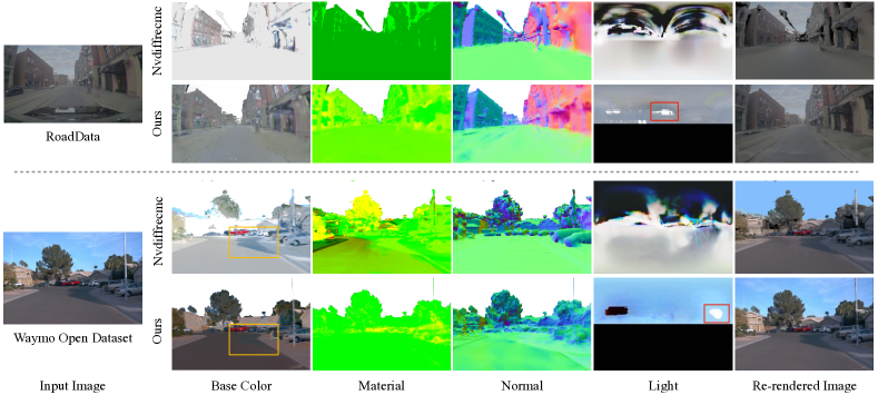
Driving dataset is challenging in several aspects: (i) The scenes are large (up to $200\text{m}\times 200\text{m}$ in horizontal plane) with complex geometry and spatially-varying material; (ii) Environment illumination is unknown and could contain high intensity from the sun; (iii) Images are captured by a fast-moving vehicle ($\approx$ 10 m/s on WOD dataset) resulting in motion blur and HDR artifacts. Even so, our method still achieves superior intrinsic scene decomposition on both scenes, leading to photo-realistic view-synthesis results (see Fig. 4). Compared to Nvdiffrecmc [18], we reconstruct cleaner base color, more accurate geometry, and higher resolution environment maps. It is worth noting that Nvdiffrecmc is designed for "outside-looking-in" setups with 360-view coverage and does not directly work on Driving dataset without modifications. In Fig. 5 we additionally show the qualitative scene relighting results under the challenging illumination settings.

4.3 Application to virtual object insertion

Qualitative comparison

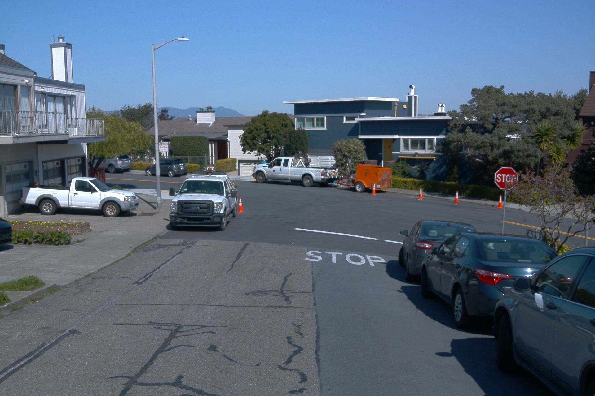
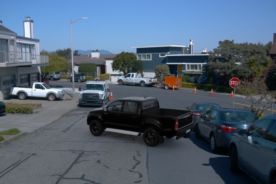
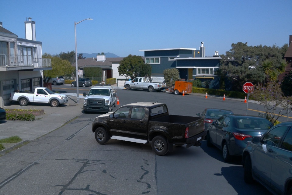
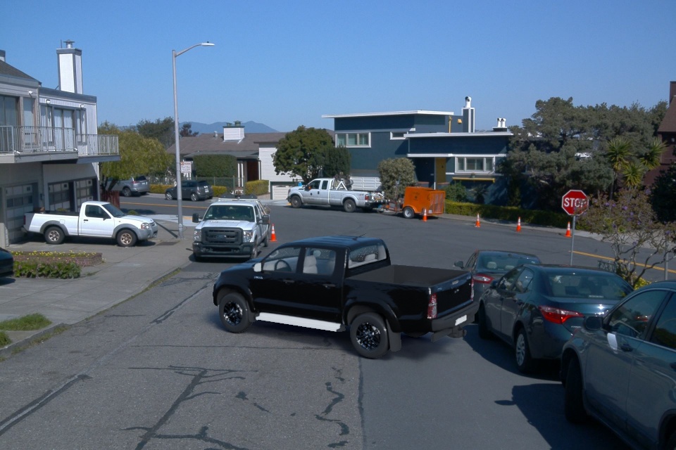
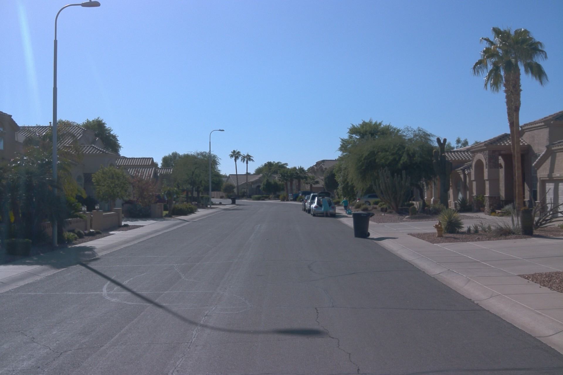
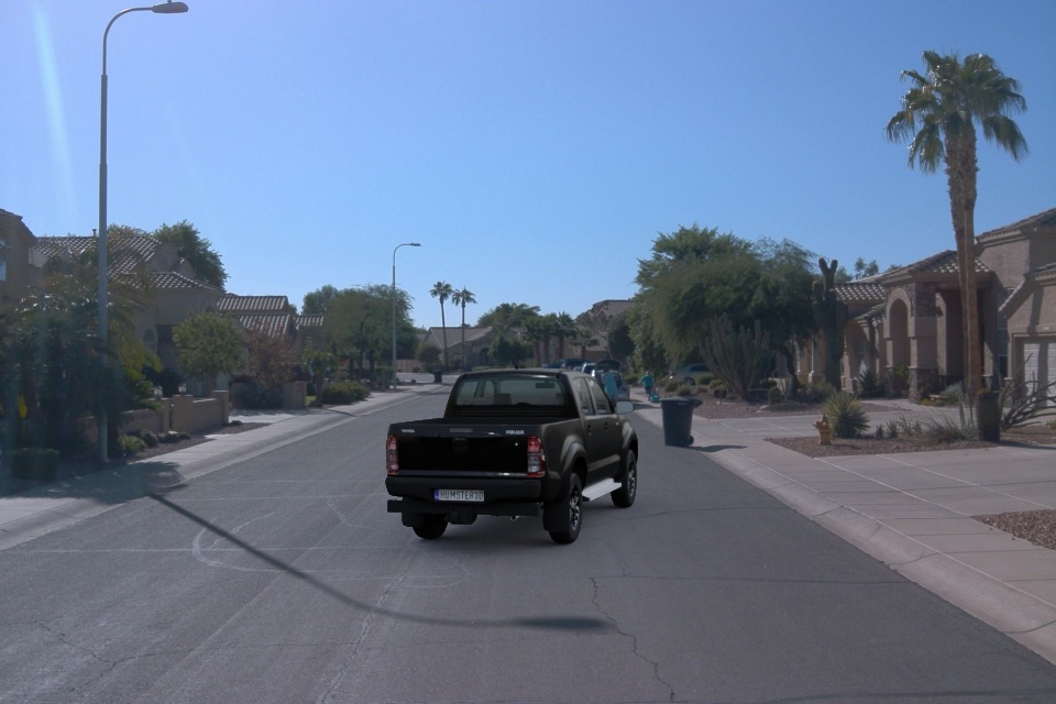
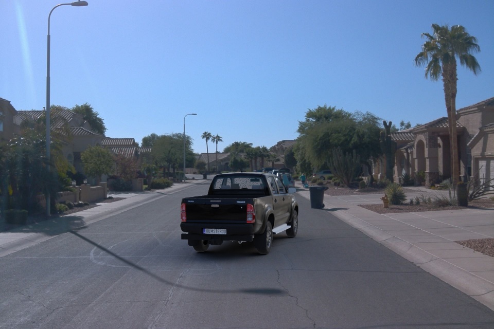
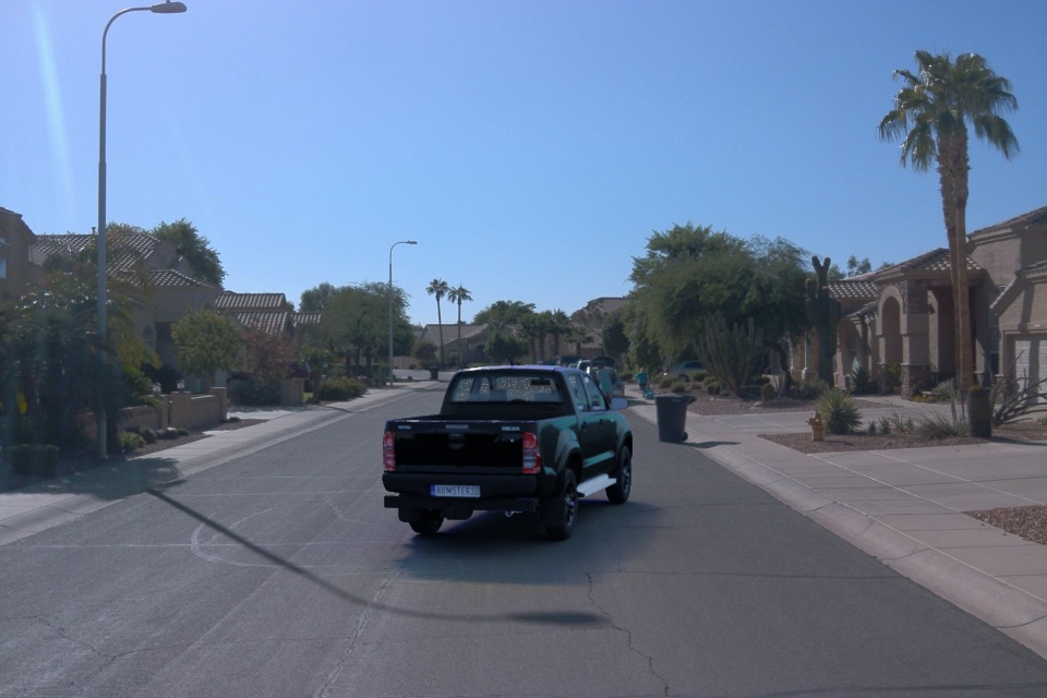
Fig. 6 shows qualitative results of object insertion on Driving dataset. FEGR is capable of faithfully representing the location of the sun, resulting in cast shadows that agree with the surroundings and yield a photo-realistic insertion.

User study

	% Ours is preferred
vs Hold-Geoffroy et al. [19]	$86.2$ %
vs Wang et al. [52]	$68.9$ %

Table 2: User study results of object insertion quality. Users consistently prefer ours over results from baseline methods.

To quantitatively evaluate the object insertion results of FEGR against other baselines, we conduct a user study using Amazon Mechanical Turk. In particular, we show the participants two augmented images with the same car inserted by our method and by the baseline in random order, and ask them to evaluate which one is more photo-realistic based on: (i) the quality of cast shadows, and (ii) the quality of reflections. For each baseline comparison, we invite 9 users to judge 29 examples and use the majority vote for the preference for each example. The results of the user study are presented in Tab. 2. A significant majority of the participants agree that FEGR yields more realistic results than all baselines, indicating a more accurate lighting estimation of our method.

5 Conclusion

We introduced FEGR, a novel hybrid rendering pipeline for inverse rendering of large urban scenes. FEGR combines high-resolution of the neural fields with the efficiency of explicit mesh representations and is capable of extracting the scene geometry, spatially varying materials, and HDR lighting from a set of posed camera images. The formulation of FEGR is flexible and it supports both single and multi-illumination data. We demonstrated that FEGR consistently outperforms SoTA methods across various challenging datasets. Finally, we have demonstrated that FEGR can seamlessly support various scene manipulations including relighting and virtual object insertion (AR).

Limitations

While FEGR makes an important step forward in neural rendering of large urban scenes, it naturally also has limitations. Inverse rendering is a highly-ill posed problem in which the solution spaces has to be constrained, especially when operating on single illumination data. We currently rely on manually designed priors to define regularization terms. In the future we would like to explore ways of learning these priors from the abundance of available data. Similar to most methods based on neural fields, FEGR is currently limited to static scenes. A promising extension in the future could incorporate advances in dynamic NeRFs [15] to mitigate this problem.

References

- [1] Harry Barrow, J Tenenbaum, A Hanson, and E Riseman. Recovering intrinsic scene characteristics. Comput. Vis. Syst, 2:3–26, 1978.
- [2] Sean Bell, Kavita Bala, and Noah Snavely. Intrinsic images in the wild. ACM Transactions on Graphics (TOG), 33(4):159, 2014.
- [3] Sai Bi, Zexiang Xu, Pratul Srinivasan, Ben Mildenhall, Kalyan Sunkavalli, Miloš Hašan, Yannick Hold-Geoffroy, David Kriegman, and Ravi Ramamoorthi. Neural reflectance fields for appearance acquisition. arXiv preprint arXiv:2008.03824, 2020.
- [4] Sai Bi, Zexiang Xu, Kalyan Sunkavalli, Miloš Hašan, Yannick Hold-Geoffroy, David Kriegman, and Ravi Ramamoorthi. Deep reflectance volumes: Relightable reconstructions from multi-view photometric images. In ECCV, pages 294–311. Springer, 2020.
- [5] Boming Zhao and Bangbang Yang, Zhenyang Li, Zuoyue Li, Guofeng Zhang, Jiashu Zhao, Dawei Yin, Zhaopeng Cui, and Hujun Bao. Factorized and controllable neural re-rendering of outdoor scene for photo extrapolation. In Proceedings of the 30th ACM International Conference on Multimedia, 2022.
- [6] Mark Boss, Raphael Braun, Varun Jampani, Jonathan T. Barron, Ce Liu, and Hendrik P.A. Lensch. Nerd: Neural reflectance decomposition from image collections. In ICCV, 2021.
- [7] Mark Boss, Andreas Engelhardt, Abhishek Kar, Yuanzhen Li, Deqing Sun, Jonathan T. Barron, Hendrik P.A. Lensch, and Varun Jampani. SAMURAI: Shape And Material from Unconstrained Real-world Arbitrary Image collections. In Advances in Neural Information Processing Systems (NeurIPS), 2022.
- [8] Mark Boss, Varun Jampani, Raphael Braun, Ce Liu, Jonathan T. Barron, and Hendrik P.A. Lensch. Neural-pil: Neural pre-integrated lighting for reflectance decomposition. In Advances in Neural Information Processing Systems (NeurIPS), 2021.
- [9] Mark Boss, Varun Jampani, Kihwan Kim, Hendrik P.A. Lensch, and Jan Kautz. Two-shot spatially-varying brdf and shape estimation. In CVPR, 2020.
- [10] Adrien Bousseau, Sylvain Paris, and Frédo Durand. User-assisted intrinsic images. In ACM Transactions on Graphics (TOG), volume 28, page 130. ACM, 2009.
- [11] Brent Burley. Physically-based shading at disney. 2012.
- [12] Wenzheng Chen, Huan Ling, Jun Gao, Edward Smith, Jaako Lehtinen, Alec Jacobson, and Sanja Fidler. Learning to predict 3d objects with an interpolation-based differentiable renderer. In NeurIPS, 2019.
- [13] Wenzheng Chen, Joey Litalien, Jun Gao, Zian Wang, Clement Fuji Tsang, Sameh Khalis, Or Litany, and Sanja Fidler. DIB-R++: Learning to predict lighting and material with a hybrid differentiable renderer. In NeurIPS, 2021.
- [14] Sara Fridovich-Keil, Alex Yu, Matthew Tancik, Qinhong Chen, Benjamin Recht, and Angjoo Kanazawa. Plenoxels: Radiance fields without neural networks. In CVPR, 2022.
- [15] Hang Gao, Ruilong Li, Shubham Tulsiani, Bryan Russell, and Angjoo Kanazawa. Monocular dynamic view synthesis: A reality check. In NeurIPS, 2022.
- [16] Mathieu Garon, Kalyan Sunkavalli, Sunil Hadap, Nathan Carr, and Jean-François Lalonde. Fast spatially-varying indoor lighting estimation. In CVPR, pages 6908–6917, 2019.
- [17] Roger Grosse, Micah K Johnson, Edward H Adelson, and William T Freeman. Ground truth dataset and baseline evaluations for intrinsic image algorithms. In ICCV, pages 2335–2342. IEEE, 2009.
- [18] Jon Hasselgren, Nikolai Hofmann, and Jacob Munkberg. Shape, Light, and Material Decomposition from Images using Monte Carlo Rendering and Denoising. arXiv:2206.03380, 2022.
- [19] Yannick Hold-Geoffroy, Akshaya Athawale, and Jean-François Lalonde. Deep sky modeling for single image outdoor lighting estimation. In CVPR, pages 6927–6935, 2019.
- [20] Yannick Hold-Geoffroy, Kalyan Sunkavalli, Sunil Hadap, Emiliano Gambaretto, and Jean-François Lalonde. Deep outdoor illumination estimation. In CVPR, pages 7312–7321, 2017.
- [21] James T Kajiya. The rendering equation. In Proceedings of the 13th annual conference on Computer graphics and interactive techniques, pages 143–150, 1986.
- [22] Balazs Kovacs, Sean Bell, Noah Snavely, and Kavita Bala. Shading annotations in the wild. In CVPR, pages 6998–7007, 2017.
- [23] Zhengfei Kuang, Kyle Olszewski, Menglei Chai, Zeng Huang, Panos Achlioptas, and Sergey Tulyakov. NeROIC: Neural object capture and rendering from online image collections. Computing Research Repository (CoRR), abs/2201.02533, 2022.
- [24] Edwin H Land and John J McCann. Lightness and retinex theory. Josa, 61(1):1–11, 1971.
- [25] Chloe LeGendre, Wan-Chun Ma, Graham Fyffe, John Flynn, Laurent Charbonnel, Jay Busch, and Paul Debevec. Deeplight: Learning illumination for unconstrained mobile mixed reality. In CVPR, pages 5918–5928, 2019.
- [26] Quewei Li, Jie Guo, Yang Fei, Feichao Li, and Yanwen Guo. Neulighting: Neural lighting for free viewpoint outdoor scene relighting with unconstrained photo collections. In Soon Ki Jung, Jehee Lee, and Adam W. Bargteil, editors, SIGGRAPH Asia 2022 Conference Papers, SA 2022, Daegu, Republic of Korea, December 6-9, 2022, pages 13:1–13:9. ACM, 2022.
- [27] Zhengqin Li, Mohammad Shafiei, Ravi Ramamoorthi, Kalyan Sunkavalli, and Manmohan Chandraker. Inverse rendering for complex indoor scenes: Shape, spatially-varying lighting and svbrdf from a single image. In CVPR, pages 2475–2484, 2020.
- [28] Zhengqi Li and Noah Snavely. Cgintrinsics: Better intrinsic image decomposition through physically-based rendering. In ECCV, pages 371–387, 2018.
- [29] Zhengqin Li, Zexiang Xu, Ravi Ramamoorthi, Kalyan Sunkavalli, and Manmohan Chandraker. Learning to reconstruct shape and spatially-varying reflectance from a single image. ACM Transactions on Graphics (TOG), 37(6):1–11, 2018.
- [30] Zhengqin Li, Ting-Wei Yu, Shen Sang, Sarah Wang, Sai Bi, Zexiang Xu, Hong-Xing Yu, Kalyan Sunkavalli, Miloš Hašan, Ravi Ramamoorthi, et al. Openrooms: An end-to-end open framework for photorealistic indoor scene datasets. arXiv preprint arXiv:2007.12868, 2020.
- [31] Andrew Liu, Shiry Ginosar, Tinghui Zhou, Alexei A. Efros, and Noah Snavely. Learning to factorize and relight a city. In ECCV, 2020.
- [32] William E. Lorensen and Harvey E. Cline. Marching cubes: A high resolution 3d surface construction algorithm. SIGGRAPH Comput. Graph., 21(4):163–169, aug 1987.
- [33] Ricardo Martin-Brualla, Noha Radwan, Mehdi S. M. Sajjadi, Jonathan T. Barron, Alexey Dosovitskiy, and Daniel Duckworth. NeRF in the Wild: Neural Radiance Fields for Unconstrained Photo Collections. In arXiv, 2020.
- [34] Ben Mildenhall, Pratul P Srinivasan, Matthew Tancik, Jonathan T Barron, Ravi Ramamoorthi, and Ren Ng. Nerf: Representing scenes as neural radiance fields for view synthesis. arXiv preprint arXiv:2003.08934, 2020.
- [35] Thomas Müller, Alex Evans, Christoph Schied, and Alexander Keller. Instant neural graphics primitives with a multiresolution hash encoding. ACM Transactions on Graphics (TOG), 41(4):102:1–102:15, July 2022.
- [36] Jacob Munkberg, Jon Hasselgren, Tianchang Shen, Jun Gao, Wenzheng Chen, Alex Evans, Thomas Mueller, and Sanja Fidler. Extracting Triangular 3D Models, Materials, and Lighting From Images. arXiv:2111.12503, 2021.
- [37] Merlin Nimier-David, Zhao Dong, Wenzel Jakob, and Anton Kaplanyan. Material and lighting reconstruction for complex indoor scenes with texture-space differentiable rendering. 2021.
- [38] Merlin Nimier-David, Delio Vicini, Tizian Zeltner, and Wenzel Jakob. Mitsuba 2: A retargetable forward and inverse renderer. ACM Transactions on Graphics (TOG), 38(6), Dec. 2019.
- [39] Steven G. Parker, James Bigler, Andreas Dietrich, Heiko Friedrich, Jared Hoberock, David Luebke, David McAllister, Morgan McGuire, Keith Morley, Austin Robison, and Martin Stich. Optix: A general purpose ray tracing engine. ACM Trans. Graph., 29(4), jul 2010.
- [40] Viktor Rudnev, Mohamed Elgharib, William Smith, Lingjie Liu, Vladislav Golyanik, and Christian Theobalt. Nerf for outdoor scene relighting. In ECCV, 2022.
- [41] Soumyadip Sengupta, Jinwei Gu, Kihwan Kim, Guilin Liu, David W. Jacobs, and Jan Kautz. Neural inverse rendering of an indoor scene from a single image. In ICCV, 2019.
- [42] Pratul P. Srinivasan, Boyang Deng, Xiuming Zhang, Matthew Tancik, Ben Mildenhall, and Jonathan T. Barron. Nerv: Neural reflectance and visibility fields for relighting and view synthesis. In CVPR, 2021.
- [43] Cheng Sun, Min Sun, and Hwann-Tzong Chen. Direct voxel grid optimization: Super-fast convergence for radiance fields reconstruction. In CVPR, 2022.
- [44] Pei Sun, Henrik Kretzschmar, Xerxes Dotiwalla, Aurelien Chouard, Vijaysai Patnaik, Paul Tsui, James Guo, Yin Zhou, Yuning Chai, Benjamin Caine, et al. Scalability in perception for autonomous driving: Waymo open dataset. In CVPR, 2020.
- [45] Matthew Tancik, Vincent Casser, Xinchen Yan, Sabeek Pradhan, Ben Mildenhall, Pratul Srinivasan, Jonathan T. Barron, and Henrik Kretzschmar. Block-NeRF: Scalable large scene neural view synthesis. arXiv, 2022.
- [46] Jiajun Tang, Yongjie Zhu, Haoyu Wang, Jun-Hoong Chan, Si Li, and Boxin Shi. Estimating spatially-varying lighting in urban scenes with disentangled representation. In ECCV, 2022.
- [47] Andrew Tao, Karan Sapra, and Bryan Catanzaro. Hierarchical multi-scale attention for semantic segmentation. arXiv preprint arXiv:2005.10821, 2020.
- [48] Haithem Turki, Deva Ramanan, and Mahadev Satyanarayanan. Mega-nerf: Scalable construction of large-scale nerfs for virtual fly-throughs. In CVPR, pages 12922–12931, June 2022.
- [49] Eric Veach and Leonidas J Guibas. Optimally combining sampling techniques for monte carlo rendering. In Proceedings of the 22nd annual conference on Computer graphics and interactive techniques, pages 419–428, 1995.
- [50] Dor Verbin, Peter Hedman, Ben Mildenhall, Todd Zickler, Jonathan T. Barron, and Pratul P. Srinivasan. Ref-NeRF: Structured view-dependent appearance for neural radiance fields. CVPR, 2022.
- [51] Peng Wang, Lingjie Liu, Yuan Liu, Christian Theobalt, Taku Komura, and Wenping Wang. Neus: Learning neural implicit surfaces by volume rendering for multi-view reconstruction. NeurIPS, 2021.
- [52] Zian Wang, Wenzheng Chen, David Acuna, Jan Kautz, and Sanja Fidler. Neural light field estimation for street scenes with differentiable virtual object insertion. In ECCV, 2022.
- [53] Zian Wang, Jonah Philion, Sanja Fidler, and Jan Kautz. Learning indoor inverse rendering with 3d spatially-varying lighting. In ICCV, 2021.
- [54] Felix Wimbauer, Shangzhe Wu, and Christian Rupprecht. De-rendering 3d objects in the wild. In CVPR, 2022.
- [55] Yuanbo Xiangli, Linning Xu, Xingang Pan, Nanxuan Zhao, Anyi Rao, Christian Theobalt, Bo Dai, and Dahua Lin. Bungeenerf: Progressive neural radiance field for extreme multi-scale scene rendering. In ECCV, 2022.
- [56] Yao Yao, Jingyang Zhang, Jingbo Liu, Yihang Qu, Tian Fang, David McKinnon, Yanghai Tsin, and Long Quan. Neilf: Neural incident light field for physically-based material estimation. In European Conference on Computer Vision (ECCV), 2022.
- [57] Ye Yu and William AP Smith. Inverserendernet: Learning single image inverse rendering. In CVPR, 2019.
- [58] Jinsong Zhang, Kalyan Sunkavalli, Yannick Hold-Geoffroy, Sunil Hadap, Jonathan Eisenman, and Jean-François Lalonde. All-weather deep outdoor lighting estimation. In CVPR, pages 10158–10166, 2019.
- [59] Jason Y. Zhang, Gengshan Yang, Shubham Tulsiani, and Deva Ramanan. NeRS: Neural reflectance surfaces for sparse-view 3d reconstruction in the wild. In Conference on Neural Information Processing Systems, 2021.
- [60] Kai Zhang, Fujun Luan, Zhengqi Li, and Noah Snavely. Iron: Inverse rendering by optimizing neural sdfs and materials from photometric images. In CVPR, 2022.
- [61] Kai Zhang, Fujun Luan, Qianqian Wang, Kavita Bala, and Noah Snavely. PhySG: Inverse rendering with spherical gaussians for physics-based material editing and relighting. In CVPR, 2021.
- [62] Kai Zhang, Gernot Riegler, Noah Snavely, and Vladlen Koltun. Nerf++: Analyzing and improving neural radiance fields, 2020.
- [63] Xiuming Zhang, Pratul P Srinivasan, Boyang Deng, Paul Debevec, William T Freeman, and Jonathan T Barron. Nerfactor: Neural factorization of shape and reflectance under an unknown illumination. ACM Transactions on Graphics (TOG), 40(6):1–18, 2021.
- [64] Yuanqing Zhang, Jiaming Sun, Xingyi He, Huan Fu, Rongfei Jia, and Xiaowei Zhou. Modeling indirect illumination for inverse rendering. In CVPR, 2022.
- [65] Qi Zhao, Ping Tan, Qiang Dai, Li Shen, Enhua Wu, and Stephen Lin. A closed-form solution to retinex with nonlocal texture constraints. 34(7):1437–1444, 2012.
- [66] Yongjie Zhu, Yinda Zhang, Si Li, and Boxin Shi. Spatially-varying outdoor lighting estimation from intrinsics. In CVPR, 2021.