Global Well-Posedness of the Primitive Equations of Large-Scale Ocean Dynamics with the Gent-McWilliams-Redi Eddy Parametrization Model

Peter Korn1, Edriss S. Titi2
(1 Max Planck Institute for Meteorology, Hamburg, Germany
2 Department of Mathematics, Texas A$\&$M University, College Station, TX 77843, USA
and
Department of Applied Mathematics and Theoretical Physics, University of Cambridge CB3 0WA, UK
)

We prove global well-posedness of the ocean primitive equations coupled to advection-diffusion equations of the oceanic tracers temperature and salinity that are supplemented by the eddy parametrization model due to Gent-McWilliams and Redi. This parametrization forms a milestone in global ocean modelling and constitutes a central part of any general ocean circulation model computation. The eddy parametrization adds a secondary transport velocity to the tracer equation and renders the original Laplacian operators in the advection-diffusion equations nonlinear, with a diffusion matrix that depends via the equation of state in a nonlinear fashion on both tracers simultaneously. The eddy parametrization of Gent-McWilliams-Redi adds complexity to the mathematical analysis of the whole system which we present here. We prove first that weak solutions exists globally in time, provided the parametrization uses a regularized density. Then we prove through a detailed analysis of the eddy operators the global well-posedness result for the ocean primitive equations with eddy parametrization. Our results apply also to the β€œsmall-slope approximation” that is commonly used in global ocean simulations.

1 Introduction

The hydrostatic Boussinesq equations of the ocean, also referred to as the ocean primitive equations, are the classical dynamical equations used in ocean and climate research (see e.g. [24, 21]). A central component is the subgridscale parametrization of mesoscale eddies due to Gent-McWilliams and Redi. This parametrization is a major achievement in the science of ocean modelling [6] and forms a cornerstone of global ocean modelling. Virtually every global ocean general circulation model relies on, and incorporates, this parametrization (see e.g. [21]). The mathematical analysis of the ocean primitive equations with the Gent-McWilliams-Redi parametrization forms the topic of this paper.

The ocean primitive equations model the large-scale circulation of the ocean as a thin layer of a weakly compressible fluid on a rotating sphere under the Boussinesq and the hydrostatic approximation. The ocean primitive equations consist of a coupled system of evolution equations for horizontal velocity $v=(v_{1},v_{2})$, potential temperature $\theta$ and salinity $S$ that is closed by an equation of state that describes the density as function of temperature, salinity and static pressure. In this work we investigate the ocean primitive equations with Gent-McWilliams-Redi eddy parametrization, which in cartesian coordinates is given by

$\displaystyle\partial_{t}v+(v\cdot\nabla)v+w\partial_{z}v+\nabla p+f\vec{k}\times v-\frac{1}{Re_{1}}\triangle\,v-\frac{1}{Re_{2}}\partial^{2}_{zz}v=0,$ (1a)
$\displaystyle\partial_{z}p+g\rho=0,$ (1b)
$\displaystyle\nabla\cdot v+\partial_{z}w=0,$ (1c)
βˆ‚tΞΈ+(vβ‹…βˆ‡)​θ+wβ€‹βˆ‚zΞΈ+𝔇𝕂i​s​o​(ρ~,KI,KD)​(ΞΈ)+𝔇𝕂G​M​(ρ~,ΞΊ)​(ΞΈ)=0,subscriptπ‘‘πœƒβ‹…π‘£βˆ‡πœƒπ‘€subscriptπ‘§πœƒsubscript𝔇subscriptπ•‚π‘–π‘ π‘œ~𝜌subscript𝐾𝐼subscriptπΎπ·πœƒsubscript𝔇subscript𝕂𝐺𝑀~πœŒπœ…πœƒ0\displaystyle\partial_{t}\theta+(v\cdot\nabla)\theta+w\partial_{z}\theta+\mathfrak{D}_{\mathbb{K}_{iso}}({\tilde{\rho}},K_{I},K_{D})(\theta)+\mathfrak{D}_{\mathbb{K}_{GM}}({\tilde{\rho}},\kappa)(\theta)=0, (1d)
βˆ‚tS+(vβ‹…βˆ‡)​S+wβ€‹βˆ‚zS+𝔇𝕂i​s​o​(ρ~,KI,KD)​(S)+𝔇𝕂G​M​(ρ~,ΞΊ)​(S)=0,subscriptπ‘‘π‘†β‹…π‘£βˆ‡π‘†π‘€subscript𝑧𝑆subscript𝔇subscriptπ•‚π‘–π‘ π‘œ~𝜌subscript𝐾𝐼subscript𝐾𝐷𝑆subscript𝔇subscript𝕂𝐺𝑀~πœŒπœ…π‘†0\displaystyle\partial_{t}S+(v\cdot\nabla)S+w\partial_{z}S+\mathfrak{D}_{\mathbb{K}_{iso}}({\tilde{\rho}},K_{I},K_{D})(S)+\mathfrak{D}_{\mathbb{K}_{GM}}({\tilde{\rho}},\kappa)(S)=0, (1e)

with the equation of state $\rho=\rho(\theta,S,p_{st})$, where $p_{st}$ denotes the static pressure (see (4) ), $w$ the vertical velocity, $\rho$ the equation of state, $f$ the Coriolis parameter, and $g$ the gravitational constant. The numbers $Re_{1},Re_{2}$ denote horizontal and vertical viscosity, $K_{I},K_{D}$ are the isoneutral and dianeutral diffusivity, $\kappa$ is referred to as eddy advection parameter. The operators $\nabla,\nabla\cdot$ and $\triangle$ denote the horizontal gradient, divergence and Laplacian, respectively.

The above system (1) differs from the classical primitive equations by introducing in the temperature and salinity equations (1d), (1e) the isoneutral eddy diffusion operator 𝔇𝕂i​s​osubscript𝔇subscriptπ•‚π‘–π‘ π‘œ\mathfrak{D}_{\mathbb{K}_{iso}} and the eddy advection operator $\mathfrak{D}_{\mathbb{K}_{GM}}$ that together implement the mesoscale eddy parametrization. Therefore in comparison to the classical analysis of the primitive equations these differences pose the main challenge in the mathematical analysis of this paper.

The work presented here capitalizes on the large body of literature of the mathematical analysis of the classical primitive equations, pioneered by Lions-Temam-Wang [31], where the global existence of weak solutions was proven. Cao-Titi established in [4] global existence and uniqueness of strong solutions for initial data in the Sobolev space $H^{1}$ and with Neumann boundary conditions for velocity on top and bottom of the domain. A different proof is given by Kobelkov [25]. For Dirichlet boundary conditions well-posedness in $H^{1}$ was obtained by Kukavica -Ziane [28]. A $L^{p}$-approach for the primitive equation was developed in Hieber-Kashiwabara [22]. The extension of global well-posedness to nonlinear equations of state can be found in Korn [26].

The ocean modelling literature is flexible about the exact specifications in the mathematical definitions of the operators 𝔇𝕂i​s​o,𝔇𝕂G​Msubscript𝔇subscriptπ•‚π‘–π‘ π‘œsubscript𝔇subscript𝕂𝐺𝑀\mathfrak{D}_{\mathbb{K}_{iso}},\mathfrak{D}_{\mathbb{K}_{GM}}. Instead the research has focused on the diffusivity parameters $K_{I},K_{D},\kappa$ and the affect of these parameter on the simulated ocean circulation (see e.g. [8, 10, 36]). In the mathematical literature the advective part $\mathfrak{D}_{\mathbb{K}_{GM}}$ was used in [1] to study the hydrostatic limit of stratified flows without viscosity. Our work investigates the mathematical structure of this important ocean parametrization in the context of global ocean modelling.

We establish first the existence of weak solutions. Here the advective part (the β€œGM-part”) necessitates the regularization of the density inside the eddy parametrization. In the small slope approximation of the eddy parametrization a regularization is not necessary to prove existence of weak solutions. For well-posedness in the Sobolev space $H^{1}$ we follow the approach of Cao-Titi [4]. The additional regularity of strong solutions necessitates a $L^{\infty}_{t}H^{1}_{x}$-bound on temperature and salinity, for which we need the following three results:

  1. (i)

    An elliptic regularity result for the isoneutral diffusion operator 𝔇𝕂i​s​osubscript𝔇subscriptπ•‚π‘–π‘ π‘œ\mathfrak{D}_{\mathbb{K}_{iso}}, this is proven in Lemma 4.7.

  2. (ii)

    A $H^{2}$ -bound on the time derivative of the isoneutral slopes to deal with the time-dependency of the coefficients of 𝔇𝕂i​s​osubscript𝔇subscriptπ•‚π‘–π‘ π‘œ\mathfrak{D}_{\mathbb{K}_{iso}}. This is established in Lemma 4.5 and requires a density regularization by which we gain two derivatives.

  3. (iii)

    A $L^{\infty}_{t}H^{1}_{x}$-bound on the eddy-induced transport velocity (see (LABEL:PROOF_STRONG_SOLUTION_3), (LABEL:PROOF_STRONG_SOLUTION_3vert)). For this estimate we need a regularization by which we gain three derivatives.

The necessary density regularization is a consequence of the nonlinear combination of derivatives in the eddy parametrization. This accumulation of derivatives poses an analytical challenge for the regularity theory, while on the discrete level, it tends to produce grid scale noise. Numerical ocean codes use smoothing procedures to prevent the noise and to compute smooth subgrid scale fluxes of density that agree with the physical expectations (see e.g. [30, 20]). Our work is also intended to inform the construction of numerical schemes of the eddy parametrization.

Organization of the paper. Section 2 provides physical background on mesoscale eddies and parametrizations. Section 3 defines the thermodynamcial concept. In section 4 we introduces the regularized eddy operators. Section 5 contains the main result, of this paper. The proofs are given in Sections 5.2 and 5.4.

2 Physical and Modelling Background

Eddy-Parametrization and Thermodynamics.

Mesoscale eddies have a typical horizontal size between 10-100km and a lifetime between 10-100 days. They belong to the most energetic phenomena in the circulation of the world’s ocean and are also referred to as β€œweather" of the ocean due to their analogy with atmospheric weather systems. They are predominantly created by baroclinic instabilities on a scale that is determined by the Rossby deformation radius. Ocean eddies are much smaller than their atmospheric counterparts and global ocean general circulation models have to invest significant computational resources to resolve parts of the mesoscale eddy spectrum.

The purpose of the eddy-induced diffusion is to mimic the behaviour of eddies to enhance mixing locally preferably along directions in which a water parcel can move in an adiabatic way without changing buoyancy (see e.g. [13] for a review). The diffusion along the isoneutral direction is by orders of magnitude larger than the diffusion perpendicular to this directions [29]. The parametrization of eddy-induced advection by Gent-McWilliams-Redi aims to capture the effect of mesoscale eddies on tracers by means of stirring through an adiabatic and potential energy reducing closure ([15], [16], [35]). Eddies convert potential into kinetic energy, thereby flattening of neutral surfaces reduces potential energy, while preserving the mass between isoneutral surfaces.

The eddy advection, originally formulated by Gent-McWilliams in isoycnal vertical coordinates [15], was transformed to depth-coordinates in [16] and combined with the eddy-induced diffusion of Redi [33]. A common modelling framework of eddy-induced advection and diffusion was developed in [18, 19], in this form it was used in numerous ocean modelling studies (see e.g. [21, 11]. The Gent-McWilliams-Redi parametrization removes essential model biases of coarse resolution models models such as the Veronis effect (see, e.g. [14]). Among its effects is a poleward heat transport in better agreement with observations or a more realistic occurrence of convective regions (see, e.g., [7], [14]).

The eddy parametrization approximates subgrid scale fluxes of density, it is essential to use therefore an accurate equation of state. Unlike the case of atmospheric dynamics no sufficiently accurate analytical expression of the equation of state is available for oceanic dynamics. We use the equation of state TEOS-10 [23] of the Intergovernmental Oceanographic Commission, the official description of seawater properties in marine science. It provides an accurate description of seawater thermodynamics by blending the Gibbs formalism of thermodynamics with seawater measurements (see, e.g. [12]). This implies the natural condition that tracers are bounded within an admissible range given by validity of the equation of state.
Parametrizations and Regularization. The purpose of eddy parametrization to capture the mean effect of (unresolved) eddies on the resolved circulation, requires by definition to select a specific scale and to average over smaller scales. For this purpose we use a convolution in the interior of the domain, in agreement with the eddy parametrization, whose physical heuristics do not apply near the boundary such that the problem of regularization near the boundary disappears.

3 Ocean Thermodynamics

The oceanic equation of state assumes that temperature, salinity and pressure values are within the observed range of the worlds ocean. Thus, the equations of state imposes bounded tracers. Accordingly we make the following (cf. [26])

Hypothesis on Ocean Thermodynamics:

  1. 1.

    There exist intervals of physically admissible ranges for temperature $I_{\theta}:=[-K_{1},K_{2}]$, salinity $I_{S}:=[L_{1},L_{2}]$, and pressure $I_{p}:=[M_{1},M_{2}]$ with $K_{1},K_{2}$, $L_{1},L_{2},M_{1},M_{2}>0$, such that for $(x,y,z,t)\in\Omega\times[0,T]$

    $$\begin{split}\theta(x,y,z,t)\in I_{\theta},\quad S(x,y,z,t)\in I_{S},\quad p(x,y,z,t)\in I_{p}.\end{split}$$ (2)
  2. 2.

    If $\theta\in I_{\theta},{S}\in I_{S}$, $p\in I_{p}$, then the coefficients $c_{i,j,k}$ of the equation of state, defined below in (LABEL:GIBBS_SPECIFIC_rho), are determined such that the density $\rho$ stays within the admissible range

    $$\begin{split}\rho\in I_{\rho}:=[R_{1},R_{2}],\quad R_{1},R_{2}>0.\end{split}$$ (3)

For the Boussinesq approximation one replaces the density $\rho$ by a reference density $\rho_{0}>0$ in all terms of the dynamical equations except for the buoyancy term in the momentum balance and in the equation of state (see e.g. Section 2.4. in [35]). For energetic consistency one uses in the equation of state the static pressure

$$\begin{split}p_{st}(z):=-g\rho_{0}z,\quad\text{for }z\leq 0.\end{split}$$ (4)
Definition 3.1.

Let the hypothesis on ocean thermodynamics (2) and (3) hold.
$i)$ Define $L^{\infty}_{I_{\theta}}(\Omega):=\{\theta\in L^{\infty}(\Omega):\theta\in I_{\theta}\}$, $L^{\infty}_{I_{S}}(\Omega):=\{S\in L^{\infty}(\Omega):S\in I_{S}\}$.
$ii)$ Let $\theta\in L^{\infty}_{I_{\theta}}(\Omega),S\in L^{\infty}_{I_{S}}(\Omega)$. The density $\rho$ is given via the specific volume $\mathrm{v}$

$$\begin{split}&\rho(\theta,S,p_{st}):=\mathrm{v}(\theta,S,p_{st})^{-1},\quad\text{with }\mathrm{v}(\theta,S,p_{st}):=\sum_{i,j,k=0}^{N_{i},N_{j},N_{k}}c_{i,j,k}S^{i}\theta^{j}p_{st}^{k},\end{split}$$ (5)

with given coefficients $c_{i,j,k}\in\mathbb{R}$ (cf table K1 in [23]), $N_{i}=7,N_{j}=6,N_{k}=5$.

Lemma 3.2 (Boundedness of Potential Temperature, Salinity and Density).

Denote by $C\in\{\theta,S\}$ the solution of the tracer equation for temperature (1d) or for salinity (1e).
$i)$ Let initial conditions satisfy $C_{0}\in{V_{C}}\cap L^{\infty}_{I_{C}}(\Omega)$. Then it holds

$$C(t)\in L^{\infty}_{I_{C}}(\Omega).$$ (6)

$ii)$ Let $\theta_{0}\in{V_{\theta}}\cap L^{\infty}_{I_{\theta}}(\Omega),S_{0}\in{V_{S}}\cap L^{\infty}_{I_{S}}(\Omega)$ be initial conditions of the tracer equation for temperature (1d) and for for salinity (1e). Then it holds

$$\rho(t)\in L^{\infty}_{I_{\rho}}(\Omega).$$ (7)
Proof.

The proof under the conditions of Definition 3.1 and without eddy parametrization can be found in [26]. It is extend to the case under consideration here by Lemma 4.6 and the skew-symmetry of $\mathbb{K}_{GM}$. ∎

Lemma 3.3 ([26]).

Let $(\theta_{1},S_{1})\in L^{\infty}_{{I_{\theta}}\times I_{S}}(\Omega)$ and $(\theta_{2},S_{2})\in L^{\infty}_{{I_{\theta}}\times I_{S}}(\Omega)$ be two pairs of temperature and salinity fields, denote by $\rho_{1}(\theta_{1},S_{1})$, $\rho_{2}(\theta_{2},S_{2})$ the two associated densities. Then it holds almost everywhere in $\Omega$

$$\begin{split}&|\rho_{1}-\rho_{2}|\leq K(|\theta_{1}-\theta_{2}|+|S_{1}-S_{2}|),\end{split}$$ (8)

where $K=K(\theta_{1},\theta_{2},S_{1},S_{2},c_{i,j,k})$ is bounded.

Density Equation. For the density an evolution equation can be derived by differentiating equation (LABEL:GIBBS_SPECIFIC_rho) with respect to time. This yields

$$\begin{split}\partial_{t}\rho&=a\partial_{t}\theta+b\partial_{t}S=aF_{\theta}+bF_{S}\\ \text{with }a&:=\frac{\partial\rho}{\partial\theta},\quad b:=\frac{\partial\rho}{\partial S},\\ F_{\theta}&:=-(v\cdot\nabla)\theta-w\partial_{z}\theta-\mathfrak{D}_{\mathbb{K}_{iso}}({\tilde{\rho}})(\theta)+\mathfrak{D}_{\mathbb{K}_{GM}}({\tilde{\rho}})(\theta),\\ F_{S}&:=-(v\cdot\nabla)S-w\partial_{z}S-\mathfrak{D}_{\mathbb{K}_{iso}}({\tilde{\rho}})(S)+\mathfrak{D}_{\mathbb{K}_{GM}}({\tilde{\rho}})(S).\end{split}$$ (9)

4 Ocean Eddy Parametrization

We introduce a mathematical formalization of oceanic neutral physics in section 4.1. This forms the basis of the definition of the eddy parametrizations in 4.2.

4.1 Regularized Isoneutral Slopes

Refer to caption
Figure 1: Illustration of the domain near the boundary. In $\Omega_{0}$, at a distance of at least $2\eta$ away from the boundary the isoneutral slope ${\bf L}$ are not modified by the cut-off function $\pi_{\partial\Omega}$. At a distance less than $2\eta$ and more than $\eta$, in $\Omega_{1}$, the slope ${\bf L}$ is reduced by the cut-off function $\pi_{\partial\Omega}$, at a distance less than $\eta$, in $\Omega_{2}$ both vanish due to the cut-off function.

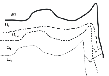
The eddy parametrizations acts in the interior of the ocean and away from the boundary and only if a minimal stratification exists. For this purpose we decompose the domain according to the distance to the boundary (see Fig. 1)

$$\begin{split}\Omega=\Omega_{0}\cup\Omega_{1}\cup\Omega_{2},\end{split}$$ (10)

with $\Omega_{0}:=\{(x,y,z)\in\Omega:\,dist((x,y,z),\partial\Omega)\geq 2\eta\}$, Ξ©1:={(x,y,z)∈Ω:Ξ·<d​i​s​t​((x,y,z),βˆ‚Ξ©)<2​η}assignsubscriptΞ©1conditional-setπ‘₯π‘¦π‘§Ξ©πœ‚π‘‘π‘–π‘ π‘‘π‘₯𝑦𝑧Ω2πœ‚\Omega_{1}:=\{(x,y,z)\in\Omega:\,\eta<dist((x,y,z),\partial\Omega)<2\eta\} and $\Omega_{2}:=\{(x,y,z)\in\Omega:\,dist((x,y,z),\partial\Omega)\leq\eta\}$. Furthermore we define the sets

$$\begin{split}{{\Omega}_{0,1}}:=&\Omega_{0}\cup\Omega_{1}=\{(x,y,z)\in\Omega:\,dist((x,y,z),\partial\Omega)>\eta\},\\ \text{and }\ {{\Omega}_{\scriptstyle 1,2}}:=&\{(x,y,z)\in\Omega:\,dist((x,y,z),\partial\Omega)>\frac{\eta}{2}\},\end{split}$$ (11)

in such a way that the boundary $\partial{{\Omega}_{\scriptstyle 1,2}}$ is of class $C^{2}$. We use the β€œcut-off” function” $\pi_{\partial\Omega}$ to define isoneutral slopes in the interior ocean. Let $\xi:[0,\infty]\to[0,1]$ be a $C^{\infty}$ monotonic nondecreasing function

ξ​(s)={0,if0≀s<1,1,ifsβ‰₯2.πœ‰π‘ casesotherwise0if0𝑠1otherwise1if𝑠2\begin{split}\xi(s)=\begin{cases}&0,\quad\text{if}\quad 0\leq s<1,\\ &1,\quad\text{if}\quad s\geq 2.\end{cases}\end{split} (12)

Define for a given $\eta>0$ and $(x,y,z)\in\bar{\Omega}$ the cut-off function

Ο€βˆ‚Ξ©β€‹(x,y,z):=ξ​(d​i​s​t​((x,y,z),βˆ‚Ξ©)Ξ·).assignsubscriptπœ‹Ξ©π‘₯π‘¦π‘§πœ‰π‘‘π‘–π‘ π‘‘π‘₯π‘¦π‘§Ξ©πœ‚\begin{split}\pi_{\partial\Omega}(x,y,z):=\xi(\frac{dist((x,y,z),\partial\Omega)}{\eta}).\end{split} (13)

The physical requirement of a minimal stratification is implemented by the tapering function Ξ s0,Ο΅0subscriptΞ subscript𝑠0subscriptitalic-Ο΅0\Pi_{s_{0},\epsilon_{0}} in Definition 4.1.

Definition 4.1 (Regularized Neutral Physics).

Suppose $\theta\in{H^{1}(\Omega)}\cap L^{\infty}_{I_{\theta}}(\Omega),S\in{H^{1}(\Omega)}\cap L^{\infty}_{I_{S}}(\Omega)$.
i)i) Let j∈Cβˆžβ€‹(Ξ©)𝑗superscript𝐢Ωj\in C^{\infty}(\Omega) be a regularizing kernel with j>0𝑗0j>0 on ΩΩ\Omega, ∫Ωj​𝑑x=1subscriptΩ𝑗differential-dπ‘₯1\int_{\Omega}j\,dx=1, jη​(x):=Ξ·βˆ’3​j​(2​xΞ·)assignsubscriptπ‘—πœ‚π‘₯superscriptπœ‚3𝑗2π‘₯πœ‚j_{\eta}(x):=\eta^{-3}j(\frac{2x}{\eta}). Define for density ρ∈LIΟβˆžβ€‹(Ξ©)𝜌subscriptsuperscript𝐿subscript𝐼𝜌Ω\rho\in L^{\infty}_{I_{\rho}}(\Omega) the
regularized density ρ~~𝜌{\tilde{\rho}} by

$$\begin{split}{\tilde{\rho}}(x,y,z):=\begin{cases}&\int_{\Omega}j_{\eta}(x-\tilde{x},y-\tilde{y},z-\tilde{z})\rho(\tilde{x},\tilde{y},\tilde{z})\,d\tilde{x}d\tilde{y}d\tilde{z},\ \text{ for }(x,y,z)\in{{\Omega}_{\scriptstyle 1,2}},\\ &0,\quad\text{ else}.\end{cases}\end{split}$$ (14)

$ii)$ We define the isoneutral slope vector ${\bf L}:={\bf L}({\tilde{\rho}}):=({L}_{x}({\tilde{\rho}}),{L}_{y}({\tilde{\rho}}))$ with respect to the density ${\tilde{\rho}}$ by

𝐋​(x,y,z,t):=𝐋​(ρ~)​(x,y,z,t):={βˆ‡hρ~​(x,y,z,t)βˆ‚zρ~​(x,y,z,t)β€‹Ο€βˆ‚Ξ©β€‹Ξ s0,Ο΅0​(|βˆ‚zρ~​(x,y,z,t)|),for ​(x,y,z)βˆˆΞ©βˆ–N​(βˆ‚zρ~),0​else,Β assign𝐋π‘₯𝑦𝑧𝑑𝐋~𝜌π‘₯𝑦𝑧𝑑assigncasesotherwisesubscriptβˆ‡β„Ž~𝜌π‘₯𝑦𝑧𝑑subscript𝑧~𝜌π‘₯𝑦𝑧𝑑subscriptπœ‹Ξ©subscriptΞ subscript𝑠0subscriptitalic-Ο΅0subscript𝑧~𝜌π‘₯𝑦𝑧𝑑otherwiseforΒ π‘₯𝑦𝑧Ω𝑁subscript𝑧~𝜌otherwise0else,Β \begin{split}{\bf L}(x,y,z,t):={\bf L}({\tilde{\rho}})(x,y,z,t):=\begin{cases}&\frac{\nabla_{h}{\tilde{\rho}}(x,y,z,t)}{\partial_{z}{\tilde{\rho}}(x,y,z,t)}\pi_{\partial\Omega}\Pi_{s_{0},\epsilon_{0}}\big{(}|\partial_{z}{\tilde{\rho}}(x,y,z,t)|\big{)},\\ &\text{for }(x,y,z)\in\Omega\setminus N(\partial_{z}{\tilde{\rho}}),\\ &0\ \text{else, }\end{cases}\end{split} (15)

with $N(\partial_{z}{\tilde{\rho}}):=\{(x,y,z)\in\Omega:|\partial_{z}{\tilde{\rho}}(x,y,z)|\leq s_{0}-\epsilon_{0}\}$, $s_{0}>\epsilon_{0}>0$, and Ξ s0,Ο΅0:[0,∞)β†’[0,1]:subscriptΞ subscript𝑠0subscriptitalic-Ο΅0β†’001\Pi_{s_{0},\epsilon_{0}}:[0,\infty)\to[0,1] a monotonic non-decreasing $C^{\infty}$-function that satisfies

Ξ s0,Ο΅0​(x)={1,forxβ‰₯s0,0,for0≀x≀s0βˆ’Ο΅0.subscriptΞ subscript𝑠0subscriptitalic-Ο΅0π‘₯casesotherwise1forπ‘₯subscript𝑠0otherwise0for0π‘₯subscript𝑠0subscriptitalic-Ο΅0\begin{split}\Pi_{s_{0},\epsilon_{0}}(x)=\begin{cases}&1,\quad\text{for}\quad x\geq s_{0},\\ &0,\quad\text{for}\quad 0\leq x\leq s_{0}-\epsilon_{0}.\end{cases}\end{split} (16)

The numbers $s_{0},\epsilon_{0}$ denote the minimal required stratification and width of the transition zone in which we reduce the slope.

4.2 Eddy-Induced Diffusion and Advection of Tracers

In this section we introduce the eddy operators 𝔇𝕂i​s​osubscript𝔇subscriptπ•‚π‘–π‘ π‘œ\mathfrak{D}_{\mathbb{K}_{iso}} and $\mathfrak{D}_{\mathbb{K}_{GM}}$ that define eddy-induced diffusion and advection.

Definition 4.2 (Eddy Operators).

Let $\theta\in{H^{1}(\Omega)}\cap L^{\infty}_{I_{\theta}}(\Omega),S\in{H^{1}(\Omega)}\cap L^{\infty}_{I_{S}}(\Omega)$ be admissible temperature and salinity fields with associated isoneutral slope vector ${\bf L}={\bf L}({\tilde{\rho}})=({L}_{x}({\tilde{\rho}}),{L}_{y}({\tilde{\rho}}))$, defined in (15).
$i)$ The isoneutral diffusion operator 𝔇𝕂i​s​o​(ρ~)subscript𝔇subscriptπ•‚π‘–π‘ π‘œ~𝜌\mathfrak{D}_{\mathbb{K}_{iso}}({\tilde{\rho}}) is for $C\in\{\theta,S\}$ defined by

𝔇𝕂i​s​o​(ρ~)​(C):=βˆ’βˆ‡3β‹…(𝕂i​s​o​(ρ~)β€‹βˆ‡3C),assignsubscript𝔇subscriptπ•‚π‘–π‘ π‘œ~πœŒπΆβ‹…subscriptβˆ‡3subscriptπ•‚π‘–π‘ π‘œ~𝜌subscriptβˆ‡3𝐢\displaystyle\mathfrak{D}_{\mathbb{K}_{iso}}({\tilde{\rho}})(C):=-\nabla_{3}\cdot\big{(}\mathbb{K}_{iso}({\tilde{\rho}})\nabla_{3}C\big{)}, (17)
with 𝕂i​s​o​(ρ~):=KI1+𝐋2​(1+δ​Lx2+Ly2(Ξ΄βˆ’1)​Lx​Ly(1βˆ’Ξ΄)​Lx(Ξ΄βˆ’1)​Lx​Ly1+Lx2+δ​Ly2(1βˆ’Ξ΄)​Ly(1βˆ’Ξ΄)​Lx(1βˆ’Ξ΄)​LyΞ΄+𝐋2),assignsubscriptπ•‚π‘–π‘ π‘œ~𝜌subscript𝐾𝐼1superscript𝐋2matrix1𝛿superscriptsubscript𝐿π‘₯2superscriptsubscript𝐿𝑦2𝛿1subscript𝐿π‘₯subscript𝐿𝑦1𝛿subscript𝐿π‘₯𝛿1subscript𝐿π‘₯subscript𝐿𝑦1superscriptsubscript𝐿π‘₯2𝛿superscriptsubscript𝐿𝑦21𝛿subscript𝐿𝑦1𝛿subscript𝐿π‘₯1𝛿subscript𝐿𝑦𝛿superscript𝐋2\displaystyle\mathbb{K}_{iso}({\tilde{\rho}}):=\frac{K_{I}}{1+{\bf L}^{2}}\begin{pmatrix}1+\delta{L}_{x}^{2}+{L}_{y}^{2}&(\delta-1){L}_{x}{L}_{y}&(1-\delta){L}_{x}\\ (\delta-1){L}_{x}{L}_{y}&1+{L}_{x}^{2}+\delta{L}_{y}^{2}&(1-\delta){L}_{y}\\ (1-\delta){L}_{x}&(1-\delta){L}_{y}&\delta+{\bf L}^{2}\end{pmatrix}, (18)

where $\delta:=\frac{K_{D}}{K_{I}}<<1$ is the fraction of isoneutral and dianeutral mixing coefficients $K_{D},K_{I}>0$ and ${\bf L}^{2}:={\bf L}\cdot{\bf L}$ .
$ii)$ The operator of eddy-induced advection $\mathfrak{D}_{\mathbb{K}_{GM}}$ is for $C\in\{\theta,S\}$ defined by

$\displaystyle\mathfrak{D}_{\mathbb{K}_{GM}}({\tilde{\rho}})(C):=\nabla_{3}\cdot\big{(}\mathbb{K}_{GM}({\tilde{\rho}})\nabla C\big{)}$ (19)
with $\displaystyle\mathbb{K}_{GM}({\tilde{\rho}}):=\kappa\begin{pmatrix}0&0&-{L}_{x}\\ 0&0&-{L}_{y}\\ {L}_{x}&{L}_{y}&0\end{pmatrix}\quad\kappa>0.$ (20)

The eddy-induced transport velocity is defined as

$$\begin{split}{v}^{*}:=-\partial_{z}(\kappa{\bf L}),\text{ and }w^{*}:=\nabla\cdot(\kappa{\bf L})\ \text{on }{{\Omega}_{0,1}}.\end{split}$$ (21)
Remark 4.3.

If the slope ${\bf L}(x,y,z,t)$ is reduced to zero then the isoneutral diffusion operator 𝔇𝕂i​s​osubscript𝔇subscriptπ•‚π‘–π‘ π‘œ\mathfrak{D}_{\mathbb{K}_{iso}} locally reduces to an anisotropic Laplacian operator with horizontal diffusivity $K_{I}>0$, vertical diffusivity $K_{D}>0$, the eddy advection operator $\mathfrak{D}_{\mathbb{K}_{GM}}$ vanishes.

Remark 4.4 (EddyAdvection).

The advective part of the eddy parametrization approximates the eddy transport of oceanic tracers in terms of the β€œeddy-induced transport velocity” $v_{3}^{\circ}=(v^{\circ},w^{\circ})$ such that $\overline{v^{\prime}C^{\prime}}\sim v_{3}^{\circ}C$, where the overbar denotes the mean and the primed variables the fluctuations. The eddy-induced velocity $v_{3}^{\circ}$ is determined from a stream function $\Psi=(\Psi^{x},\Psi^{y},0)$ by $v_{3}^{\circ}=curl\Psi$ and $\Psi:=\vec{z}\times\kappa{\bf L}$. A direct calculation shows that $v^{\circ}\cdot\nabla_{3}C=-\nabla_{3}\cdot(\mathbb{K}_{GM}\nabla_{3}C)$.

4.3 Small Slope Approximation

In simulations of the real ocean, numerical circulation models use for efficiency reasons the β€œsmall slope approximation” of isoneutral diffusion (see [15])

$$\begin{split}\mathbb{K}_{iso}^{small}:=K_{I}\begin{pmatrix}1&0&{L}_{x}^{\circ}\\ 0&1&{L}_{y}^{\circ}\\ {L}_{x}^{\circ}&{L}_{y}^{\circ}&\delta+|{\bf L}^{\circ}|^{2}\end{pmatrix},\quad\mathbb{K}_{GM}^{small}:=\kappa\begin{pmatrix}0&0&-{L}_{x}^{\circ}\\ 0&0&-{L}_{y}^{\circ}\\ {L}_{x}^{\circ}&{L}_{y}^{\circ}&0\end{pmatrix},\end{split}$$ (22)

where for an chosen parameter $r<<1$ the β€œsmall slopes” are defined by

$$\begin{split}{\bf L}^{\circ}:=\begin{cases}&{\bf L}\quad\text{if }|{\bf L}|<r,\\ &0\quad\text{else}.\end{cases}\end{split}$$ (23)

This approximation is justified by the observation that in the world ocean horizontal density gradients are generally smaller than vertical density gradients, therefore the off-diagonal terms in (18) can be neglected (see [17], Chapter. 14).

We define the eddy operators in the small slope approximation accordingly as

$$\begin{split}\mathfrak{D}_{\mathbb{K}_{iso}^{small}}({\tilde{\rho}})(C):=\nabla_{3}\cdot(\mathbb{K}_{iso}^{small}\nabla_{3}C),\quad\mathfrak{D}_{\mathbb{K}_{GM}^{small}}({\tilde{\rho}})(C):=\nabla_{3}\cdot(\mathbb{K}_{GM}^{small}\nabla_{3}C).\end{split}$$ (24)

4.4 Properties of the Eddy Parametrization

Lemma 4.5.

Let $\theta\in L^{2}_{loc}([0,T],{V_{\theta}}\cap L^{\infty}_{I_{\theta}}(\Omega)),S\in\L^{2}_{loc}([0,T],{V_{S}}\cap L^{\infty}_{I_{S}}(\Omega))$.
$i)$ The isoneutral slope satisfies ${\bf L}\in L^{\infty}([0,T],H^{s}(\Omega))$, $s\geq 0$, and

$$\begin{split}||{\bf L}||_{H^{s}({{\Omega}_{0,1}})}\leq||\rho||^{2}_{L^{2}(\Omega)}.\end{split}$$ (25)

$ii)$ Let $(v,\theta,S)$ be a strong solution of (56) (cf. Def. 5.1 $i)$. Then $\partial_{t}{\bf L}\in L^{\infty}([0,T],H^{s}(\Omega))$, $s\geq 0$, and a continuous function $K_{L}(t)$ exists such that

$$\begin{split}&||\partial_{t}{\bf L}(t)||_{H^{s}({{\Omega}_{0,1}})}\leq K_{L}(t).\end{split}$$ (26)

$iii)$ Let two pairs of temperature and salinity fields $(\theta_{1},S_{1})$, $(\theta_{2},S_{2})\in L^{2}_{loc}([0,T],{V_{\theta}}\cap L^{\infty}_{I_{\theta}}(\Omega))\times L^{2}_{loc}([0,T],{V_{S}}\cap L^{\infty}_{I_{S}}(\Omega))$ be given. For the slopes ${\bf L}({\tilde{\rho}}_{1}),{\bf L}({\tilde{\rho}}_{2})$ it holds

$\displaystyle||{\bf L}({\tilde{\rho}}_{1})(t)-{\bf L}({\tilde{\rho}}_{2})(t)||_{L^{\infty}(\Omega)}\leq c\tau(\frac{c}{s_{0}}+\frac{C}{s_{0}^{2}})|I_{\rho}|||\rho_{1}(t)-\rho_{2}(t)||_{{L^{2}(\Omega)}},$ (27)
Proof.

$Ad\,i)$ We decompose the domain ${{\Omega}_{0,1}}=I_{1}\cup I_{2}\cup I_{3}$, where $I_{1}:=\{(x,y,z)\in{{\Omega}_{0,1}}:\,|\partial_{z}{\tilde{\rho}}(x,y,z)|\geq s_{0}\}$, $I_{2}:=\{(x,y,z)\in{{\Omega}_{0,1}}:\,s_{0}-\epsilon\leq|\partial_{z}{\tilde{\rho}}(x,y,z)|\leq s_{0}\}$, $I_{3}:=\{(x,y,z)\in{{\Omega}_{0,1}}:\,0\leq|\partial_{z}{\tilde{\rho}}(x,y,z)|<s_{0}-\epsilon\}$. These sets are measurable, since $\partial_{z}{\tilde{\rho}}$ is continuous. Using this decomposition we find with $l\in\mathbb{N}^{3}$,

‖𝐋‖Hs​(Ξ©0,1)2=βˆ‘|l|≀s∫I1|Dl​(βˆ‡hρ~βˆ‚zρ~)|2​𝑑x​𝑑y​𝑑z+∫I2|Dl​(βˆ‡hρ~βˆ‚zρ~​Πs0,Ο΅0​(|βˆ‚zρ~|))|2​𝑑x​𝑑y​𝑑z,superscriptsubscriptnorm𝐋superscript𝐻𝑠subscriptΞ©012subscript𝑙𝑠subscriptsubscript𝐼1superscriptsuperscript𝐷𝑙subscriptβˆ‡β„Ž~𝜌subscript𝑧~𝜌2differential-dπ‘₯differential-d𝑦differential-d𝑧subscriptsubscript𝐼2superscriptsuperscript𝐷𝑙subscriptβˆ‡β„Ž~𝜌subscript𝑧~𝜌subscriptΞ subscript𝑠0subscriptitalic-Ο΅0subscript𝑧~𝜌2differential-dπ‘₯differential-d𝑦differential-d𝑧\begin{split}||{\bf L}||_{H^{s}({{\Omega}_{0,1}})}^{2}&=\sum_{|l|\leq s}\int_{I_{1}}|D^{l}\big{(}\frac{\nabla_{h}{\tilde{\rho}}}{\partial_{z}{\tilde{\rho}}}\big{)}|^{2}\,dxdydz+\int_{I_{2}}|D^{l}\big{(}\frac{\nabla_{h}{\tilde{\rho}}}{\partial_{z}{\tilde{\rho}}}\Pi_{s_{0},\epsilon_{0}}(|\partial_{z}{\tilde{\rho}}|)\big{)}|^{2}\,dxdydz,\end{split} (28)

where the integral over $I_{3}$ vanishes due to the tapering by Ξ s0,Ο΅0subscriptΞ subscript𝑠0subscriptitalic-Ο΅0\Pi_{s_{0},\epsilon_{0}}. For the first integral we obtain with the Leibniz rule, the commutation of convolution and differentiation for $k\in\mathbb{N}^{3}$

$$\begin{split}&\int_{I_{1}}|D^{l}{\bf L}|^{2}\,dxdydz=\sum_{|k|\leq l}\int_{I_{1}}|D^{k}(\nabla_{h}{\tilde{\rho}})D^{l-k}((\partial_{z}{\tilde{\rho}})^{-1})|^{2}\,dxdydz\\ &\leq c\sum_{|k|\leq l}\int_{I_{1}}|(\rho\ast D^{k+1}j_{\eta})(\rho\ast D^{l-k+1}j_{\eta})|^{2}\,dxdydz\leq c||\rho||_{L^{2}(\Omega)}^{4}.\end{split}$$ (29)

An analogous estimate follows for the second integral in (28), with an upper bound $c>0$ that depends in addition on Ξ s0,Ο΅0subscriptΞ subscript𝑠0subscriptitalic-Ο΅0\Pi_{s_{0},\epsilon_{0}}.
$Ad\,ii)$ For the $H^{s}$-norm of the time derivative follows with $l\in\mathbb{N}^{3}$, and by using the same decomposition of ${{\Omega}_{0,1}}=I_{1}\cup I_{2}\cup I_{3}$ as in part $i)$

β€–βˆ‚t𝐋‖Hs​(Ξ©0,1)2=βˆ‘|l|≀s∫I1|Dlβ€‹βˆ‚t(βˆ‡hρ~βˆ‚zρ~)|2​𝑑x​𝑑y​𝑑z+∫I2|Dlβ€‹βˆ‚t(βˆ‡hρ~βˆ‚zρ~​Πs0,Ο΅0​(|βˆ‚zρ~|))|2​𝑑x​𝑑y​𝑑z.superscriptsubscriptnormsubscript𝑑𝐋superscript𝐻𝑠subscriptΞ©012subscript𝑙𝑠subscriptsubscript𝐼1superscriptsuperscript𝐷𝑙subscript𝑑subscriptβˆ‡β„Ž~𝜌subscript𝑧~𝜌2differential-dπ‘₯differential-d𝑦differential-d𝑧subscriptsubscript𝐼2superscriptsuperscript𝐷𝑙subscript𝑑subscriptβˆ‡β„Ž~𝜌subscript𝑧~𝜌subscriptΞ subscript𝑠0subscriptitalic-Ο΅0subscript𝑧~𝜌2differential-dπ‘₯differential-d𝑦differential-d𝑧\begin{split}||\partial_{t}{\bf L}||_{H^{s}({{\Omega}_{0,1}})}^{2}&=\sum_{|l|\leq s}\int_{I_{1}}|D^{l}\partial_{t}\big{(}\frac{\nabla_{h}{\tilde{\rho}}}{\partial_{z}{\tilde{\rho}}}\big{)}|^{2}\,dxdydz+\int_{I_{2}}|D^{l}\partial_{t}\big{(}\frac{\nabla_{h}{\tilde{\rho}}}{\partial_{z}{\tilde{\rho}}}\Pi_{s_{0},\epsilon_{0}}(|\partial_{z}{\tilde{\rho}}|)\big{)}|^{2}\,dxdydz.\end{split} (30)

For the first integral on the right-hand side we obtain with with the Leibniz rule

$$\begin{split}&\sum_{|l|\leq s}\int_{I_{1}}|D^{l}\partial_{t}\big{(}\frac{\nabla_{h}{\tilde{\rho}}}{\partial_{z}{\tilde{\rho}}}\big{)}|^{2}\,dxdydz=\sum_{|l|\leq s}\int_{I_{1}}|D^{l}\big{(}\frac{\partial_{z}{\tilde{\rho}}\partial_{t}\nabla_{h}{\tilde{\rho}}-\nabla_{h}{\tilde{\rho}}\partial_{t}\partial_{z}{\tilde{\rho}}}{|\partial_{z}{\tilde{\rho}}|^{2}}\big{)}|^{2}\,dxdydz\\ &=\sum_{|l|\leq s}\int_{I_{1}}|D^{l}\ (g)D^{l-k}(h^{-1}))|^{2}\,dxdydz,\end{split}$$ (31)

with $g:=\partial_{z}{\tilde{\rho}}\partial_{t}\nabla_{h}{\tilde{\rho}}-\nabla_{h}{\tilde{\rho}}\partial_{t}\partial_{z}{\tilde{\rho}}$, and $h^{-1}:=|\partial_{z}{\tilde{\rho}}|^{-2}$. For the first term of $g$ we derive with the Leibniz rule,

$$\begin{split}&|D^{l}(\partial_{x_{j}}{\tilde{\rho}}\partial_{t}\partial_{x_{i}}{\tilde{\rho}})|=|\sum_{|n|\leq|l|}\big{(}\rho\ast(D^{n}\partial_{x_{j}}j_{\eta})\big{)}\big{(}\partial_{t}\rho\ast(D^{l-n}\partial_{x_{i}}j_{\eta})\big{)}|\\ &=|\sum_{|n|\leq|l|}\big{(}\rho\ast J_{1}^{n,j}\big{)}\big{(}\partial_{t}\rho\ast J_{1}^{n-l,i}\big{)}|\leq c|\rho|\sum_{|n|\leq|l|}|\partial_{t}\rho\ast J_{1}^{n-l,i}|\end{split}$$ (32)

with $J_{1}^{n,i}:=D^{n}\partial_{x_{i}}j_{\eta}\in C^{\infty}(\Omega)$. An analogous estimate holds for the second term of the function $g$. For the function $h$ we obtain from the chain rule

$$\begin{split}&|D^{k}(\frac{1}{h})|=|\sum_{j=1}^{|k|}\sum_{|n|=j}c_{k}\frac{D^{n}\partial_{z}{\tilde{\rho}}}{\partial_{z}{\tilde{\rho}}^{j+1}}|\leq\sum_{j=1}^{|k|}\sum_{|n|=j}|\frac{c_{k}}{s_{0}^{j+1}}\rho\ast J_{1}^{n,i}|\leq K|\rho|,\end{split}$$ (33)

where $K$ depends on constants $c_{k}\in\mathbb{R}$ and on the stratification $s_{0}$.

We estimate now in (LABEL:COROLLARY_SLOPES_1_PF_3a) the term with the time derivative of density by the evolution equation (9) for density. We claim that a continuous, time-dependent function $M$ exist, such that

$$\begin{split}&\int_{I_{1}}|(\partial_{t}\rho)\ast J_{1}^{n-l}|^{2}\,dxdydz=\int_{I_{1}}|(aF_{\theta}+bF_{S})\ast J_{1}^{n-l}|^{2}\,dxdydz\leq M(t).\end{split}$$ (34)

For $aF_{\theta}$ follows with the boundedness of the thermal expansion function $a$

∫I1|(a​FΞΈ)βˆ—J1nβˆ’l|2​𝑑x​𝑑y​𝑑z=∫I1|(a​d​i​v3​(v​θ+(𝕂i​s​o​(ρ~)+𝕂G​M​(ρ~))β€‹βˆ‡3ΞΈ))βˆ—J1nβˆ’l|2​𝑑x​𝑑y​𝑑z≀‖aβ€–Lβˆžβ€‹(Ξ©)2β€‹βˆ«I1|(v​θ+(𝕂i​s​o​(ρ~)+𝕂G​M​(ρ~))β€‹βˆ‡3ΞΈ)βˆ—βˆ‡3J1nβˆ’l|2​𝑑x​𝑑y​𝑑z≀MΞΈ,subscriptsubscript𝐼1superscriptβˆ—π‘ŽsubscriptπΉπœƒsuperscriptsubscript𝐽1𝑛𝑙2differential-dπ‘₯differential-d𝑦differential-d𝑧subscriptsubscript𝐼1superscriptβˆ—π‘Žπ‘‘π‘–subscript𝑣3π‘£πœƒsubscriptπ•‚π‘–π‘ π‘œ~𝜌subscript𝕂𝐺𝑀~𝜌subscriptβˆ‡3πœƒsuperscriptsubscript𝐽1𝑛𝑙2differential-dπ‘₯differential-d𝑦differential-d𝑧superscriptsubscriptnormπ‘Žsuperscript𝐿Ω2subscriptsubscript𝐼1superscriptβˆ—π‘£πœƒsubscriptπ•‚π‘–π‘ π‘œ~𝜌subscript𝕂𝐺𝑀~𝜌subscriptβˆ‡3πœƒsubscriptβˆ‡3superscriptsubscript𝐽1𝑛𝑙2differential-dπ‘₯differential-d𝑦differential-d𝑧subscriptπ‘€πœƒ\begin{split}&\int_{I_{1}}|(aF_{\theta})\ast J_{1}^{n-l}|^{2}\,dxdydz\\ &=\int_{I_{1}}|\big{(}adiv_{3}(v\theta+(\mathbb{K}_{iso}({\tilde{\rho}})+\mathbb{K}_{GM}({\tilde{\rho}}))\nabla_{3}\theta)\big{)}\ast J_{1}^{n-l}|^{2}\,dxdydz\\ &\leq||a||_{L^{\infty}(\Omega)}^{2}\int_{I_{1}}|\big{(}v\theta+(\mathbb{K}_{iso}({\tilde{\rho}})+\mathbb{K}_{GM}({\tilde{\rho}}))\nabla_{3}\theta\big{)}\ast\nabla_{3}J_{1}^{n-l}|^{2}\,dxdydz\leq M_{\theta},\end{split} (35)

here $M_{\theta}(t)$ denotes a continuous function that dominates the integral in (LABEL:COROLLARY_SLOPES_1_PF_4a), because the integrand is a convolution of an integrable function with a regularizing kernel and therefore smooth and bounded. Analogously follows for $bF_{S}$ in (LABEL:COROLLARY_SLOPES_1_PF_4) that $\int_{I_{1}}|bF_{S}\ast J_{1}^{n-l}|^{2}\,dxdydz\leq M_{S}$. With $M:=M_{\theta}+M_{S}$ the asserted inequality (LABEL:COROLLARY_SLOPES_1_PF_4) follows. From (LABEL:COROLLARY_SLOPES_1_PF_4), (LABEL:COROLLARY_SLOPES_1_PF_3b), (LABEL:COROLLARY_SLOPES_1_PF_3a) and (LABEL:COROLLARY_SLOPES_1_PF_3) follows that the first term in (30) satisfies the assertion. The boundedness of the second term follows analogously.
$Ad\,iii)$ From the continuity of Ξ s0,Ο΅0subscriptΞ subscript𝑠0subscriptitalic-Ο΅0\Pi_{s_{0},\epsilon_{0}}, and the regularity properties of ${\tilde{\rho}}$ follows

$$\begin{split}&|{\bf L}_{2}-{\bf L}_{1}|\leq(\frac{c}{s_{0}}+\frac{C}{s_{0}^{2}})||\nabla_{h}{\tilde{\rho}}_{1}||_{{H^{2}({{\Omega}_{0,1}})}}||\partial_{z}({\tilde{\rho}}_{1}-{\tilde{\rho}}_{2})||_{{H^{2}({{\Omega}_{0,1}})}}\\ &+\frac{C}{s_{0}^{2}}||\partial_{z}{\tilde{\rho}}_{1}||_{{H^{2}({{\Omega}_{0,1}})}}||\nabla({\tilde{\rho}}_{1}-{\tilde{\rho}}_{2})||_{{H^{2}({{\Omega}_{0,1}})}}\leq c\tau(\frac{c}{s_{0}}+\frac{C}{s_{0}^{2}})|I_{\rho}|||\rho_{1}(t)-\rho_{2}(t)||_{{L^{2}(\Omega)}}.\end{split}$$

∎

Lemma 4.6 (Ellipticity of 𝕂i​s​osubscriptπ•‚π‘–π‘ π‘œ\mathbb{K}_{iso}).

Let a isoneutral slope vector ${\bf L}_{0}:={\bf L}({\tilde{\rho}}_{0})$ be given. The isoneutral operator 𝔇𝕂i​s​osubscript𝔇subscriptπ•‚π‘–π‘ π‘œ\mathfrak{D}_{\mathbb{K}_{iso}} satisfies for $\theta\in{H^{1}(\Omega)}\cap L^{\infty}_{I_{\theta}}(\Omega),S\in{H^{1}(\Omega)}\cap L^{\infty}_{I_{S}}(\Omega)$ the following inequalities

$\displaystyle\mu||\nabla_{3}\theta||_{{L^{2}(\Omega)}}^{2}+k_{\theta}\int_{\Gamma_{u}}|\theta(x,y,0)|^{2}\,dxdy$
β‰€βˆ«Ξ©π”‡π•‚i​s​o​(ρ~0)​(ΞΈ)​θ​𝑑x​𝑑y​𝑑z≀Mβ€‹β€–βˆ‡3ΞΈβ€–L2​(Ξ©)2+kΞΈβ€‹βˆ«Ξ“u|θ​(x,y,0)|2​𝑑x​𝑑yabsentsubscriptΞ©subscript𝔇subscriptπ•‚π‘–π‘ π‘œsubscript~𝜌0πœƒπœƒdifferential-dπ‘₯differential-d𝑦differential-d𝑧𝑀superscriptsubscriptnormsubscriptβˆ‡3πœƒsuperscript𝐿2Ξ©2subscriptπ‘˜πœƒsubscriptsubscriptΓ𝑒superscriptπœƒπ‘₯𝑦02differential-dπ‘₯differential-d𝑦\displaystyle\leq\int_{\Omega}\mathfrak{D}_{\mathbb{K}_{iso}}({\tilde{\rho}}_{0})(\theta)\theta\,dxdydz\leq M||\nabla_{3}\theta||_{{L^{2}(\Omega)}}^{2}+k_{\theta}\int_{\Gamma_{u}}|\theta(x,y,0)|^{2}\,dxdy
and ΞΌβ€‹β€–βˆ‡3Sβ€–L2​(Ξ©)2β‰€βˆ«Ξ©π”‡π•‚i​s​o​(ρ~0)​(S)​S​𝑑x​𝑑y​𝑑z≀Mβ€‹β€–βˆ‡3Sβ€–L2​(Ξ©)2,πœ‡superscriptsubscriptnormsubscriptβˆ‡3𝑆superscript𝐿2Ξ©2subscriptΞ©subscript𝔇subscriptπ•‚π‘–π‘ π‘œsubscript~𝜌0𝑆𝑆differential-dπ‘₯differential-d𝑦differential-d𝑧𝑀superscriptsubscriptnormsubscriptβˆ‡3𝑆superscript𝐿2Ξ©2\displaystyle\mu||\nabla_{3}S||_{{L^{2}(\Omega)}}^{2}\leq\int_{\Omega}\mathfrak{D}_{\mathbb{K}_{iso}}({\tilde{\rho}}_{0})(S)S\,dxdydz\leq M||\nabla_{3}S||_{{L^{2}(\Omega)}}^{2},
with $\displaystyle\mu:=min\{K_{I},K_{D}\},M:=max\{K_{I},K_{D}\}.$ (36)
Proof.

The isoneutral mixing operator 𝕂i​s​osubscriptπ•‚π‘–π‘ π‘œ\mathbb{K}_{iso} can be written as

𝕂i​s​o​(ρ~)=ℛ​(𝐋)​𝔻​ℛT​(𝐋),subscriptπ•‚π‘–π‘ π‘œ~πœŒβ„›π‹π”»superscriptℛ𝑇𝐋\begin{split}\mathbb{K}_{iso}({\tilde{\rho}})=\mathcal{R}({\bf L})\mathbb{D}\mathcal{R}^{T}({\bf L}),\end{split} (37)

where the orthogonal matrix $\mathcal{R}({\bf L})$ and the diagonal matrix $\mathbb{D}$ are given by

$$\begin{split}\mathcal{R}({\bf L}):=\begin{pmatrix}\frac{{L}_{y}}{|{\bf L}|}&\frac{{L}_{x}}{|{\bf L}|\sqrt{1+{\bf L}^{2}}}&-\frac{{L}_{x}}{\sqrt{1+{\bf L}^{2}}}\\ -\frac{{L}_{x}}{|{\bf L}|}&\frac{{L}_{y}}{|{\bf L}|\sqrt{1+{\bf L}^{2}}}&-\frac{{L}_{y}}{\sqrt{1+{\bf L}^{2}}}\\ 0&\frac{{\bf L}}{\sqrt{1+{\bf L}^{2}}}&\frac{1}{\sqrt{1+{\bf L}^{2}}}\end{pmatrix},\qquad\mathbb{D}=\begin{pmatrix}K_{I}&0&0\\ 0&K_{I}&0\\ 0&0&K_{D}\end{pmatrix}.\end{split}$$ (38)

For (36) follows after integration by parts and with (37)

βˆ«Ξ©π”‡π•‚i​s​o​(ρ~0)​(C)​C​𝑑x​𝑑y​𝑑z=∫Ω|𝔻1/2​ℛT​(𝐋0)β€‹βˆ‡3C|2​𝑑x​𝑑y​𝑑z+kCβ€‹βˆ«Ξ“u|C​(x,y,0)|2​𝑑x​𝑑y=∫ΩKI​|(β„›T​(𝐋0)β€‹βˆ‡3C)β‹…e1|2+KI​|(β„›T​(𝐋0)β€‹βˆ‡3C)β‹…e2|2+KD​|(β„›T​(𝐋0)β€‹βˆ‡3C)β‹…e3|2​d​x​d​y​d​z+kCβ€‹βˆ«Ξ“u|C​(x,y,0)|2​𝑑x​𝑑y,subscriptΞ©subscript𝔇subscriptπ•‚π‘–π‘ π‘œsubscript~𝜌0𝐢𝐢differential-dπ‘₯differential-d𝑦differential-d𝑧subscriptΞ©superscriptsuperscript𝔻12superscriptℛ𝑇subscript𝐋0subscriptβˆ‡3𝐢2differential-dπ‘₯differential-d𝑦differential-d𝑧subscriptπ‘˜πΆsubscriptsubscriptΓ𝑒superscript𝐢π‘₯𝑦02differential-dπ‘₯differential-d𝑦subscriptΞ©subscript𝐾𝐼superscriptβ‹…superscriptℛ𝑇subscript𝐋0subscriptβˆ‡3𝐢subscript𝑒12subscript𝐾𝐼superscriptβ‹…superscriptℛ𝑇subscript𝐋0subscriptβˆ‡3𝐢subscript𝑒22subscript𝐾𝐷superscriptβ‹…superscriptℛ𝑇subscript𝐋0subscriptβˆ‡3𝐢subscript𝑒32𝑑π‘₯𝑑𝑦𝑑𝑧subscriptπ‘˜πΆsubscriptsubscriptΓ𝑒superscript𝐢π‘₯𝑦02differential-dπ‘₯differential-d𝑦\begin{split}&\int_{\Omega}\mathfrak{D}_{\mathbb{K}_{iso}}({\tilde{\rho}}_{0})(C)C\,dxdydz=\int_{\Omega}|\mathbb{D}^{1/2}\mathcal{R}^{T}({\bf L}_{0})\nabla_{3}C|^{2}\,dxdydz\\ &+k_{C}\int_{\Gamma_{u}}|C(x,y,0)|^{2}\,dxdy\\ &=\int_{\Omega}K_{I}|(\mathcal{R}^{T}({\bf L}_{0})\nabla_{3}C)\cdot e_{1}|^{2}+K_{I}|(\mathcal{R}^{T}({\bf L}_{0})\nabla_{3}C)\cdot e_{2}|^{2}\\ &+K_{D}|(\mathcal{R}^{T}({\bf L}_{0})\nabla_{3}C)\cdot e_{3}|^{2}\,dxdydz+k_{C}\int_{\Gamma_{u}}|C(x,y,0)|^{2}\,dxdy,\end{split}

where $e_{i}$, $i=1,2,3,$ denotes the canonical basis in $\mathbb{R}^{3}$ and $\mathbb{D}^{1/2}:=diag(\sqrt{K_{I}},\sqrt{K_{I}},$ $\sqrt{K_{D}})$ the diagonal matrix. Since $\mathcal{R}^{T}({\bf L}_{0})$ is orthogonal, the assertion follows. ∎

Lemma 4.7 (Elliptic Estimate for Isoneutral Operator).

Let $F,G\in{L^{2}(\Omega)}$ be given. Then there exists a solution $(\theta,S)$ of the equation system

$$\begin{split}&\mathfrak{D}_{\mathbb{K}_{iso}}({\tilde{\rho}})(\theta)=F,\quad\text{ and }\quad\mathfrak{D}_{\mathbb{K}_{iso}}({\tilde{\rho}})(S)=G,\end{split}$$ (39)

with boundary conditions (53). Equation (LABEL:REDI_OP_SOLVE) is satisfied in the following sense for all $\phi^{\theta}\in{V_{\theta}}$ and $\phi^{S}\in{V_{S}}$

∫Ω(𝕂i​s​o​(ρ~)β€‹βˆ‡3ΞΈ)β‹…βˆ‡3ϕθ​d​x​d​y​d​z+kΞΈβ€‹βˆ«Ξ“uθ​ϕθ​𝑑x​𝑑y=∫ΩF​ϕθ​𝑑x​𝑑y​𝑑z,∫Ω(𝕂i​s​o​(ρ~)β€‹βˆ‡3S)β‹…βˆ‡3Ο•S​d​x​d​y​d​z=∫ΩG​ϕS​𝑑x​𝑑y​𝑑z.formulae-sequencesubscriptΞ©β‹…subscriptπ•‚π‘–π‘ π‘œ~𝜌subscriptβˆ‡3πœƒsubscriptβˆ‡3superscriptitalic-Ο•πœƒπ‘‘π‘₯𝑑𝑦𝑑𝑧subscriptπ‘˜πœƒsubscriptsubscriptΞ“π‘’πœƒsuperscriptitalic-Ο•πœƒdifferential-dπ‘₯differential-d𝑦subscriptΩ𝐹superscriptitalic-Ο•πœƒdifferential-dπ‘₯differential-d𝑦differential-d𝑧subscriptΞ©β‹…subscriptπ•‚π‘–π‘ π‘œ~𝜌subscriptβˆ‡3𝑆subscriptβˆ‡3superscriptitalic-ϕ𝑆𝑑π‘₯𝑑𝑦𝑑𝑧subscriptΩ𝐺superscriptitalic-ϕ𝑆differential-dπ‘₯differential-d𝑦differential-d𝑧\begin{split}&\int_{\Omega}(\mathbb{K}_{iso}({\tilde{\rho}})\nabla_{3}\theta)\cdot\nabla_{3}\phi^{\theta}\,dxdydz+k_{\theta}\int_{\Gamma_{u}}\theta\phi^{\theta}\,dxdy=\int_{\Omega}F\phi^{\theta}\,dxdydz,\\ &\int_{\Omega}(\mathbb{K}_{iso}({\tilde{\rho}})\nabla_{3}S)\cdot\nabla_{3}\phi^{S}\,dxdydz=\int_{\Omega}G\phi^{S}\,dxdydz.\end{split} (40)

The solution $(\theta,S)$ satisfies

$$\begin{split}||\theta||_{{{H^{2}(\Omega)}}}\leq c||\mathfrak{D}_{\mathbb{K}_{iso}}({\tilde{\rho}})(\theta)||_{{L^{2}(\Omega)}},\quad\text{and}\quad||S||_{{{H^{2}(\Omega)}}}\leq c||\mathfrak{D}_{\mathbb{K}_{iso}}({\tilde{\rho}})(S)||_{{L^{2}(\Omega)}},\end{split}$$ (41)

where $c=c(K_{I},K_{D},|\Omega|,|I_{\rho}|)$, and $|I_{\rho}|$ is the interval length of admissible density values.

Proof.

Step 1: Solvability of Linearized Equation.

We linearize (LABEL:REDI_OP_SOLVE2) by fixing an arbitrary pair $(\theta^{{}^{\prime}},S^{{}^{\prime}})\in{V_{\theta}},\times{V_{S}}$. With the associated density ${\tilde{\rho}}^{{}^{\prime}}:={\tilde{\rho}}^{{}^{\prime}}({\theta}^{{}^{\prime}},{S}^{{}^{\prime}})$ we define D𝕂i​s​o​(ρ~β€²)​(C):=βˆ‡3β‹…(𝕂i​s​o​(ρ~β€²)β€‹βˆ‡3C)assignsubscript𝐷subscriptπ•‚π‘–π‘ π‘œsuperscript~πœŒβ€²πΆβ‹…subscriptβˆ‡3subscriptπ•‚π‘–π‘ π‘œsuperscript~πœŒβ€²subscriptβˆ‡3𝐢D_{\mathbb{K}_{iso}}({\tilde{\rho}}^{{}^{\prime}})(C):=\nabla_{3}\cdot\big{(}\mathbb{K}_{iso}({{\tilde{\rho}}}^{{}^{\prime}})\nabla_{3}C\big{)}. This operator is linear, continuous and uniformly elliptic on ${{V_{\theta}}}\times{{V_{S}}}$ (cf. Prop. 4.6). The linearized equation on ${V_{\theta}}\times{V_{S}}$ reads

∫Ω(𝕂i​s​o​(ρ~β€²)β€‹βˆ‡3ΞΈ)β‹…βˆ‡3ϕθ​d​x​d​y​d​z+kΞΈβ€‹βˆ«Ξ“uθ​ϕθ​𝑑x​𝑑y=∫ΩF​ϕθ​𝑑x​𝑑y​𝑑z,∫Ω(𝕂i​s​o​(ρ~β€²)β€‹βˆ‡3S)β‹…βˆ‡3Ο•S​d​x​d​y​d​z=∫ΩG​ϕS​𝑑x​𝑑y​𝑑z.formulae-sequencesubscriptΞ©β‹…subscriptπ•‚π‘–π‘ π‘œsuperscript~πœŒβ€²subscriptβˆ‡3πœƒsubscriptβˆ‡3superscriptitalic-Ο•πœƒπ‘‘π‘₯𝑑𝑦𝑑𝑧subscriptπ‘˜πœƒsubscriptsubscriptΞ“π‘’πœƒsuperscriptitalic-Ο•πœƒdifferential-dπ‘₯differential-d𝑦subscriptΩ𝐹superscriptitalic-Ο•πœƒdifferential-dπ‘₯differential-d𝑦differential-d𝑧subscriptΞ©β‹…subscriptπ•‚π‘–π‘ π‘œsuperscript~πœŒβ€²subscriptβˆ‡3𝑆subscriptβˆ‡3superscriptitalic-ϕ𝑆𝑑π‘₯𝑑𝑦𝑑𝑧subscriptΩ𝐺superscriptitalic-ϕ𝑆differential-dπ‘₯differential-d𝑦differential-d𝑧\begin{split}&\int_{\Omega}(\mathbb{K}_{iso}({{\tilde{\rho}}}^{{}^{\prime}})\nabla_{3}\theta)\cdot\nabla_{3}\phi^{\theta}\,dxdydz+k_{\theta}\int_{\Gamma_{u}}\theta\phi^{\theta}\,dxdy=\int_{\Omega}F\phi^{\theta}\,dxdydz,\\ &\int_{\Omega}(\mathbb{K}_{iso}({{\tilde{\rho}}}^{{}^{\prime}})\nabla_{3}S)\cdot\nabla_{3}\phi^{S}\,dxdydz=\int_{\Omega}G\phi^{S}\,dxdydz.\end{split} (42)

The Lax-Milgram Lemma shows that for all fixed $\theta^{{}^{\prime}}\in{V_{\theta}},{S}^{{}^{\prime}}\in{V_{S}}$ equation (LABEL:REDI_OP_SOLVE_GALERKIN_12) has a unique weak solution $\theta=\theta({\theta}^{{}^{\prime}})\in{V_{\theta}},\,S=S({S}^{{}^{\prime}})\in{V_{S}}$, which according to elliptic regularity theory (e.g. Sect. 9.6. in [2]) satisfies

$$\begin{split}||\theta||_{{H^{2}(\Omega)}}\leq c||F||_{{L^{2}(\Omega)}}\quad\text{and}\quad||S||_{{H^{2}(\Omega)}}\leq c||G||_{{L^{2}(\Omega)}},\end{split}$$ (43)

here $c$ depends on the maximum norm $||\nabla_{3}k_{i,j}({\tilde{\rho}}^{{}^{\prime}})||_{L^{\infty}}$ of the gradient of the matrix elements $k_{i,j}({\tilde{\rho}}^{{}^{\prime}})$ of 𝕂i​s​osubscriptπ•‚π‘–π‘ π‘œ\mathbb{K}_{iso}. Since $||\nabla_{3}k_{i,j}({\tilde{\rho}}^{{}^{\prime}})||_{L^{\infty}}\leq c_{0}||\rho^{\prime}||_{L^{2}(\Omega)}\leq c_{0}|\Omega|\,|I_{\rho}|$, with $c_{0}$ depending on constants $K_{I},K_{D}$, we conclude that $c=c(K_{I},K_{D},|\Omega|,|I_{\rho}|)$. In particular is $c$ independent of $(\theta^{{}^{\prime}},S^{{}^{\prime}})\in{V_{\theta}},\times{V_{S}}$.

Step 2: Solvability of System (LABEL:REDI_OP_SOLVE2).

Consider the mapping $H$ that assigns to each fixed pair $({\theta}^{{}^{\prime}},{S}^{{}^{\prime}})\in{V_{\theta}}\times{V_{S}}$ a solution $(\theta,S)\in{{H^{2}(\Omega)}}\times{{H^{2}(\Omega)}}$ of (LABEL:REDI_OP_SOLVE_GALERKIN_12) with coefficient matrix 𝕂i​s​o​(ρ~β€²)subscriptπ•‚π‘–π‘ π‘œsuperscript~πœŒβ€²\mathbb{K}_{iso}({\tilde{\rho}}^{{}^{\prime}})

$$\begin{split}H:{V_{\theta}}\times{V_{S}}&\to{V_{\theta}}\times{V_{S}}\\ ({\theta}^{{}^{\prime}},{S}^{{}^{\prime}})&\mapsto H({\theta}^{{}^{\prime}},{S}^{{}^{\prime}}):=(\theta,S).\end{split}$$ (44)

We assert the following three properties of $H$

$$\begin{split}i)\ &H\ \text{maps a closed ball}\ B_{R}\subset{V_{\theta}}\times{V_{S}}\text{ into itself}.\\ ii)\ &H\ \text{is continuous,}\\ iii)\ &H\ \text{is compact.}\end{split}$$ (45)

$Ad\,i)$ Consider the ball $B_{R_{1}}^{\theta}\subset{V_{\theta}}$ and $B_{R_{2}}^{S}\subset{V_{S}}$ with radius $R_{1}:=c||F||_{{L^{2}(\Omega)}}$ and $R_{2}:=c||G||_{{L^{2}(\Omega)}}$, with $F,G$ and $c=c(K_{I},K_{D},|\Omega|,|I_{\rho}|)$ from (43). Choose a non-zero $(\theta_{0},S_{0})\in{V_{\theta}}\times{V_{S}}$, define ${\theta}^{{}^{\prime}}:=R_{1}\theta_{0}/||\theta_{0}||_{{H^{1}(\Omega)}}$ and ${S}^{{}^{\prime}}:=R_{2}S_{0}/||S_{0}||_{{H^{1}(\Omega)}}$. Then $({\theta}^{{}^{\prime}},{S}^{{}^{\prime}})\in B_{R}:=B_{R_{1}}^{\theta}\times B_{R_{2}}^{S}$. From (43) follows that $H({\theta}^{{}^{\prime}},{S}^{{}^{\prime}})=(\theta,S)$ satisfies $||\theta||_{{H^{2}(\Omega)}}\leq R_{1},||S||_{{{H^{2}(\Omega)}}}\leq R_{2}$. Thus $||\theta||_{{H^{1}(\Omega)}}\leq R_{1}$ and $||S||_{{H^{1}(\Omega)}}\leq R_{2}$.
$Ad\,ii)$ Let the sequence $({\theta}_{k}^{{}^{\prime}},{S}_{k}^{{}^{\prime}})_{k}\subseteq{V_{\theta}}\times{V_{S}}$ converge with respect to the $H^{1}$-topology of ${V_{\theta}}\times{V_{S}}$ to a limit $({\theta}^{{}^{\prime}},{S}^{{}^{\prime}})\in{V_{\theta}}\times{V_{S}}$ and denote the associated densities by $({\tilde{\rho}}_{k}^{{}^{\prime}})_{k}$ and ${\tilde{\rho}}{{}^{\prime}}$. For each element of $({\theta}_{k}^{{}^{\prime}},{S}_{k}^{{}^{\prime}})_{k}$ exists a solution $(\theta_{k},S_{k})_{k}:=(H({\theta}_{k}^{{}^{\prime}},{S}_{k}^{{}^{\prime}}))_{k}$ $\subseteq{V_{\theta}}\times{V_{S}}$ of (LABEL:REDI_OP_SOLVE_GALERKIN_12), i.e. for $\phi^{\theta}\in{V_{\theta}}^{m},\phi^{S}\in{V_{S}}^{m}$, $k\in\mathbb{N}$ we have

∫Ω(𝕂i​s​o​(ρ~kβ€²)β€‹βˆ‡3ΞΈk)β‹…βˆ‡3ϕθ​d​x​d​y​d​z+kΞΈβ€‹βˆ«Ξ“uΞΈk​ϕθ​𝑑x​𝑑y=∫ΩF​ϕθ​𝑑x​𝑑y​𝑑z,∫Ω(𝕂i​s​o​(ρ~kβ€²)β€‹βˆ‡3Sk)β‹…βˆ‡3Ο•S​d​x​d​y​d​z=∫ΩG​ϕS​𝑑x​𝑑y​𝑑z.formulae-sequencesubscriptΞ©β‹…subscriptπ•‚π‘–π‘ π‘œsuperscriptsubscript~πœŒπ‘˜β€²subscriptβˆ‡3subscriptπœƒπ‘˜subscriptβˆ‡3superscriptitalic-Ο•πœƒπ‘‘π‘₯𝑑𝑦𝑑𝑧subscriptπ‘˜πœƒsubscriptsubscriptΓ𝑒subscriptπœƒπ‘˜superscriptitalic-Ο•πœƒdifferential-dπ‘₯differential-d𝑦subscriptΩ𝐹superscriptitalic-Ο•πœƒdifferential-dπ‘₯differential-d𝑦differential-d𝑧subscriptΞ©β‹…subscriptπ•‚π‘–π‘ π‘œsuperscriptsubscript~πœŒπ‘˜β€²subscriptβˆ‡3subscriptπ‘†π‘˜subscriptβˆ‡3superscriptitalic-ϕ𝑆𝑑π‘₯𝑑𝑦𝑑𝑧subscriptΩ𝐺superscriptitalic-ϕ𝑆differential-dπ‘₯differential-d𝑦differential-d𝑧\begin{split}&\int_{\Omega}(\mathbb{K}_{iso}({{\tilde{\rho}}}_{k}^{{}^{\prime}})\nabla_{3}\theta_{k})\cdot\nabla_{3}\phi^{\theta}\,dxdydz+k_{\theta}\int_{\Gamma_{u}}\theta_{k}\phi^{\theta}\,dxdy=\int_{\Omega}F\phi^{\theta}\,dxdydz,\\ &\int_{\Omega}(\mathbb{K}_{iso}({{\tilde{\rho}}}_{k}^{{}^{\prime}})\nabla_{3}S_{k})\cdot\nabla_{3}\phi^{S}\,dxdydz=\int_{\Omega}G\phi^{S}\,dxdydz.\end{split} (46)

For equation (LABEL:REDI_OP_SOLVE_GALERKIN_12) with a coefficient matrix 𝕂i​s​o​(ρ~β€²)subscriptπ•‚π‘–π‘ π‘œsuperscript~πœŒβ€²\mathbb{K}_{iso}({\tilde{\rho}}^{{}^{\prime}}) given by the limit ${\tilde{\rho}}^{{}^{\prime}}$ of $({\tilde{\rho}}_{k})_{k}$ there exists a solution $(\theta^{\sharp},S^{\sharp})\in{V_{\theta}}\times{V_{S}}$ such that for $\phi^{\theta}\in{V_{\theta}},\phi^{S}\in{V_{S}}$

∫Ω(𝕂i​s​o​(ρ~β€²)β€‹βˆ‡3ΞΈβ™―)β‹…βˆ‡3ϕθ​d​x​d​y​d​z+kΞΈβ€‹βˆ«Ξ“uθ♯​ϕθ​𝑑x​𝑑y=∫ΩF​ϕθ​𝑑x​𝑑y​𝑑z,∫Ω(𝕂i​s​o​(ρ~β€²)β€‹βˆ‡3Sβ™―)β‹…βˆ‡3Ο•S​d​x​d​y​d​z=∫ΩG​ϕS​𝑑x​𝑑y​𝑑z.formulae-sequencesubscriptΞ©β‹…subscriptπ•‚π‘–π‘ π‘œsuperscript~πœŒβ€²subscriptβˆ‡3superscriptπœƒβ™―subscriptβˆ‡3superscriptitalic-Ο•πœƒπ‘‘π‘₯𝑑𝑦𝑑𝑧subscriptπ‘˜πœƒsubscriptsubscriptΓ𝑒superscriptπœƒβ™―superscriptitalic-Ο•πœƒdifferential-dπ‘₯differential-d𝑦subscriptΩ𝐹superscriptitalic-Ο•πœƒdifferential-dπ‘₯differential-d𝑦differential-d𝑧subscriptΞ©β‹…subscriptπ•‚π‘–π‘ π‘œsuperscript~πœŒβ€²subscriptβˆ‡3superscript𝑆♯subscriptβˆ‡3superscriptitalic-ϕ𝑆𝑑π‘₯𝑑𝑦𝑑𝑧subscriptΩ𝐺superscriptitalic-ϕ𝑆differential-dπ‘₯differential-d𝑦differential-d𝑧\begin{split}&\int_{\Omega}(\mathbb{K}_{iso}({{\tilde{\rho}}}^{{}^{\prime}})\nabla_{3}\theta^{\sharp})\cdot\nabla_{3}\phi^{\theta}\,dxdydz+k_{\theta}\int_{\Gamma_{u}}\theta^{\sharp}\phi^{\theta}\,dxdy=\int_{\Omega}F\phi^{\theta}\,dxdydz,\\ &\int_{\Omega}(\mathbb{K}_{iso}({{\tilde{\rho}}}^{{}^{\prime}})\nabla_{3}S^{\sharp})\cdot\nabla_{3}\phi^{S}\,dxdydz=\int_{\Omega}G\phi^{S}\,dxdydz.\end{split} (47)

We show now that the sequence of solutions $(\theta_{k},S_{k})$ of (LABEL:REDI_OP_SOLVE_GALERKIN_14c) converges to the solution $(\theta^{\sharp},S^{\sharp})$ of (LABEL:REDI_OP_SOLVE_GALERKIN_14d). After subtracting (LABEL:REDI_OP_SOLVE_GALERKIN_14d) from (LABEL:REDI_OP_SOLVE_GALERKIN_14c) we obtain for the temperature difference with 𝕂^i​s​o:=𝕂i​s​o​(ρ~kβ€²)βˆ’π•‚i​s​o​(ρ~β€²)assignsubscript^π•‚π‘–π‘ π‘œsubscriptπ•‚π‘–π‘ π‘œsuperscriptsubscript~πœŒπ‘˜β€²subscriptπ•‚π‘–π‘ π‘œsuperscript~πœŒβ€²\widehat{\mathbb{K}}_{iso}:=\mathbb{K}_{iso}({\tilde{\rho}}_{k}^{{}^{\prime}})-\mathbb{K}_{iso}({\tilde{\rho}}^{{}^{\prime}}) and for $\phi^{\theta}\in{V_{\theta}}$ that

$\displaystyle 0$ =∫Ω(𝕂i​s​o​(ρ~kβ€²)β€‹βˆ‡3ΞΈkβˆ’π•‚i​s​o​(ρ~β€²)β€‹βˆ‡3ΞΈβ™―)β‹…βˆ‡3ϕθ​d​x​d​y​d​z+kΞΈβ€‹βˆ«Ξ“u(ΞΈkβˆ’ΞΈβ™―)​ϕθ​𝑑x​𝑑yabsentsubscriptΞ©β‹…subscriptπ•‚π‘–π‘ π‘œsuperscriptsubscript~πœŒπ‘˜β€²subscriptβˆ‡3subscriptπœƒπ‘˜subscriptπ•‚π‘–π‘ π‘œsuperscript~πœŒβ€²subscriptβˆ‡3superscriptπœƒβ™―subscriptβˆ‡3superscriptitalic-Ο•πœƒπ‘‘π‘₯𝑑𝑦𝑑𝑧subscriptπ‘˜πœƒsubscriptsubscriptΓ𝑒subscriptπœƒπ‘˜superscriptπœƒβ™―superscriptitalic-Ο•πœƒdifferential-dπ‘₯differential-d𝑦\displaystyle=\int_{\Omega}\big{(}\mathbb{K}_{iso}({{\tilde{\rho}}}_{k}^{{}^{\prime}})\nabla_{3}\theta_{k}-\mathbb{K}_{iso}({{\tilde{\rho}}}^{{}^{\prime}})\nabla_{3}\theta^{\sharp}\big{)}\cdot\nabla_{3}\phi^{\theta}\,dxdydz+k_{\theta}\int_{\Gamma_{u}}(\theta_{k}-\theta^{\sharp})\phi^{\theta}\,dxdy
=∫Ω(𝕂^i​s​oβ€‹βˆ‡3ΞΈk+𝕂i​s​o​(ρ~β€²)β€‹βˆ‡3(ΞΈkβˆ’ΞΈβ™―))β‹…βˆ‡Ο•ΞΈβ€‹d​x​d​y​d​z+kΞΈβ€‹βˆ«Ξ“u(ΞΈkβˆ’ΞΈβ™―)​ϕθ​𝑑x​𝑑y.absentsubscriptΞ©β‹…subscript^π•‚π‘–π‘ π‘œsubscriptβˆ‡3subscriptπœƒπ‘˜subscriptπ•‚π‘–π‘ π‘œsuperscript~πœŒβ€²subscriptβˆ‡3subscriptπœƒπ‘˜superscriptπœƒβ™―βˆ‡superscriptitalic-Ο•πœƒπ‘‘π‘₯𝑑𝑦𝑑𝑧subscriptπ‘˜πœƒsubscriptsubscriptΓ𝑒subscriptπœƒπ‘˜superscriptπœƒβ™―superscriptitalic-Ο•πœƒdifferential-dπ‘₯differential-d𝑦\displaystyle=\int_{\Omega}\big{(}\widehat{\mathbb{K}}_{iso}\nabla_{3}\theta_{k}+\mathbb{K}_{iso}({{\tilde{\rho}}}^{{}^{\prime}})\nabla_{3}(\theta_{k}-\theta^{\sharp})\big{)}\cdot\nabla\phi^{\theta}\,dxdydz+k_{\theta}\int_{\Gamma_{u}}(\theta_{k}-\theta^{\sharp})\phi^{\theta}\,dxdy. (48)

In the first term on the right-hand of (48), the differences 𝕂^i​s​o=(k^i,j)i,jsubscript^π•‚π‘–π‘ π‘œsubscriptsubscript^π‘˜π‘–π‘—π‘–π‘—\widehat{\mathbb{K}}_{iso}=(\hat{k}_{i,j})_{i,j} can be bounded by slope differences, i.e $|\hat{k}_{i,j}|\leq c|{\bf L}({\tilde{\rho}}_{k}^{{}^{\prime}})-{\bf L}({\tilde{\rho}}^{{}^{\prime}})|$. Lemma 4.5 bounds slope differences by density differences, $|{\bf L}({\tilde{\rho}}_{k}^{{}^{\prime}})-{\bf L}({\tilde{\rho}}^{{}^{\prime}})|\leq c|{\tilde{\rho}}_{k}^{{}^{\prime}}-{\tilde{\rho}}^{{}^{\prime}}|$, and Lemma 3.3 bounds density differences by temperature, salinity differences and with the $H^{1}$-convergence of $(\theta_{k}^{{}^{\prime}},S_{k}^{{}^{\prime}})$ to $(\theta^{{}^{\prime}},S^{{}^{\prime}})$ follows

$$\begin{split}&\lim_{k\to\infty}\int_{\Omega}\big{(}\widehat{\mathbb{K}}_{iso}\nabla_{3}\theta_{k}\big{)}\cdot\nabla_{3}\phi^{\theta}\,dxdydz\\ &\leq c\lim_{k\to\infty}||\theta_{k}||_{{{H^{1}(\Omega)}}}||\phi^{\theta}||_{{H^{1}(\Omega)}}\big{(}||\theta{{}^{\prime}}-\theta_{k}^{{}^{\prime}}||_{{L^{2}(\Omega)})}+||S^{{}^{\prime}}-S_{k}^{{}^{\prime}}||_{{L^{2}(\Omega)})}\big{)}=0.\end{split}$$ (49)

For the second term on the right-hand side of (48) we derive with the ellipticity of 𝕂i​s​osubscriptπ•‚π‘–π‘ π‘œ\mathbb{K}_{iso} (cf. Lemma 4.7) and with the particular choice $\phi^{\theta}:=\theta_{k}-\theta^{\sharp}$

0β‰₯limkβ†’βˆž|∫Ω(𝕂i​s​o​(ρ~β€²)β€‹βˆ‡3(ΞΈkβˆ’ΞΈβ™―))β‹…βˆ‡3(ΞΈkβˆ’ΞΈβ™―)⁑d​x​d​y​d​z+kΞΈβ€‹βˆ«Ξ“u|ΞΈkβˆ’ΞΈβ™―|2​𝑑x​𝑑y|β‰₯μ​limkβ†’βˆž{β€–βˆ‡3(ΞΈkβˆ’ΞΈβ™―)β€–L2​(Ξ©)2+kθ​‖θk​(z=0)βˆ’ΞΈβ™―β€‹(z=0)β€–L2​(Ξ©)2}.0subscriptβ†’π‘˜subscriptΞ©β‹…subscriptπ•‚π‘–π‘ π‘œsuperscript~πœŒβ€²subscriptβˆ‡3subscriptπœƒπ‘˜superscriptπœƒβ™―subscriptβˆ‡3subscriptπœƒπ‘˜superscriptπœƒβ™―π‘‘π‘₯𝑑𝑦𝑑𝑧subscriptπ‘˜πœƒsubscriptsubscriptΓ𝑒superscriptsubscriptπœƒπ‘˜superscriptπœƒβ™―2differential-dπ‘₯differential-dπ‘¦πœ‡subscriptβ†’π‘˜superscriptsubscriptnormsubscriptβˆ‡3subscriptπœƒπ‘˜superscriptπœƒβ™―superscript𝐿2Ξ©2subscriptπ‘˜πœƒsubscriptsuperscriptnormsubscriptπœƒπ‘˜π‘§0superscriptπœƒβ™―π‘§02superscript𝐿2Ξ©\begin{split}0\geq&\lim_{k\to\infty}\big{|}\int_{\Omega}\big{(}\mathbb{K}_{iso}({{\tilde{\rho}}}^{{}^{\prime}})\nabla_{3}(\theta_{k}-\theta^{\sharp})\big{)}\cdot\nabla_{3}(\theta_{k}-\theta^{\sharp})\,dxdydz+k_{\theta}\int_{\Gamma_{u}}|\theta_{k}-\theta^{\sharp}|^{2}\,dxdy\big{|}\\ \geq&\mu\lim_{k\to\infty}\big{\{}||\nabla_{3}(\theta_{k}-\theta^{\sharp})||_{{L^{2}(\Omega)}}^{2}+k_{\theta}||\theta_{k}(z=0)-\theta^{\sharp}(z=0)||^{2}_{{L^{2}(\Omega)}}\big{\}}.\end{split} (50)

From the convergence of $(\nabla_{3}\theta_{k})_{k}$ to $\nabla\theta^{\sharp}$ in ${L^{2}(\Omega)}$ and of $(\theta_{k}(z=0))_{k}$ in $L^{2}(\Gamma_{u})$ to $\theta^{\sharp}(z=0)$ follows with Poincaré’s inequality (cf. Prop. III.2.38 in [3]) that $(\theta_{k})_{k}$ converges to $\theta^{\sharp}$ in ${H^{1}(\Omega)}$. Thus $(\theta_{k})_{k}$ converges to $\theta^{\sharp}$ in ${H^{1}(\Omega)}$. For salinity we obtain an analogous statement to (50), here the boundary term is absent due to the boundary condition for salinity. From Poincaré’s inequality (cf. Prop. III.2.39 in [3]) follows that $(S_{k})_{k}$ converges to $S^{\sharp}$ in ${H^{1}(\Omega)}$. Since $(\theta_{k},S_{k})=H({\theta}_{k}^{{}^{\prime}},{S}_{k}^{{}^{\prime}})$ and $(\theta^{\sharp},S^{\sharp})=H({\theta}^{{}^{\prime}},{S}^{{}^{\prime}})$ this proves the continuity of $H$.
$Ad\,iii)$ Consider a sequence $({\theta}_{k}^{{}^{\prime}},{S}_{k}^{{}^{\prime}})_{k}\subseteq B_{R_{1}}^{\theta}\times B_{R_{2}}^{S}$. The elements of the image sequence under $H$, $({\theta}_{k},{S}_{k}):=H({\theta}_{k}^{{}^{\prime}},{S}_{k}^{{}^{\prime}})$, solve (LABEL:REDI_OP_SOLVE_GALERKIN_12) with coefficients determined by ${\tilde{\rho}}_{k}^{{}^{\prime}}:={\tilde{\rho}}({\theta}_{k}^{{}^{\prime}},{S}_{k}^{{}^{\prime}})$. This implies that for all $k\in\mathbb{N}$ the solution $\theta_{k},{S}_{k}$ satisfies

$$\begin{split}||\theta_{k}||_{{{H^{2}(\Omega)}}}\leq c||F||_{{L^{2}(\Omega)}}\quad\text{and}\quad||S_{k}||_{{{H^{2}(\Omega)}}}\leq c||G||_{{L^{2}(\Omega)}},\end{split}$$ (51)

since $c=c(K_{I},K_{D},|\Omega|,|I_{\rho}|)$ the sequence is bounded uniformly in ${H^{2}(\Omega)}$. This implies that $(\theta_{k},S_{k})_{k}$ converges weakly in ${H^{2}(\Omega)}$. Due to the compact embedding of ${H^{2}(\Omega)}$ in ${H^{1}(\Omega)}$ there exists a subsequence $(\theta_{n},S_{n})_{n}$ that converges in ${H^{1}(\Omega)}$.

From properties $i)-iii)$ in (45) follows with the Tikhonnov-Schauder Fixed-Point Theorem that the mapping $H$ has a fix point, i.e. $H(\theta,S)=(\theta,S)$. This proves the Lemma. ∎

5 Regularity Results of Ocean Primitive Equations with Mesoscale Eddy Parametrization

We specify now boundary conditions and introduce basic function spaces. In Section 5.1 we state our main results.

Boundary Conditions.

The domain is $\Omega:=M\times(-h,0)\subseteq\mathbb{R}^{3}$, with depth $h>0$, the bottom $M\subseteq\mathbb{R}^{2}$ is a bounded domain in $\mathbb{R}^{2}$ with a boundary $\partial M$ that is a $C^{2}$-curve. The boundary $\partial\Omega=\Gamma_{s}\cup\Gamma_{b}\cup\Gamma_{u}$ consists of a lateral boundary $\Gamma_{s}:=\{(x,y,z)\in\bar{\Omega}:(x,y)\in\partial M\}$, a bottom boundary $\Gamma_{b}:=\{(x,y,z)\in\bar{\Omega}:z=-h\}$ and a surface boundary $\Gamma_{u}:=\{(x,y,z)\in\bar{\Omega}:z=0\}$. The boundary conditions follow Cao-Titi [4]. Specifically, we impose at the top a wind driven boundary condition for velocity and a rigid-lid for vertical velocity. At the side a no penetration and a stress-free boundary condition, at the bottom we employ for the horizontal velocity the stress-free boundary condition for the horizontal and a no penetration boundary condition for the vertical velocity:

$\displaystyle on\ \Gamma_{u}:\partial_{z}v=h\tau,w=0,$
$\displaystyle on\ \Gamma_{s}:\ v\cdot\vec{n}=0,\partial_{\vec{n}}v\times\vec{n}=0,w=0,$
$\displaystyle on\ \Gamma_{b}:\partial_{z}v=0,w=0,$

where $\tau$ is a given 2D wind stress field. Since the isoneutral slope vector ${\bf L}$ vanishes in the vicinity of the boundary $\partial\Omega$ only those diagonal matrix elements of 𝕂i​s​osubscriptπ•‚π‘–π‘ π‘œ\mathbb{K}_{iso} are non-vanishing that do not involve ${\bf L}$. This allows to express the tracer boundary conditions without the mixing tensor 𝕂i​s​osubscriptπ•‚π‘–π‘ π‘œ\mathbb{K}_{iso} in the following way

$\displaystyle on\ \Gamma_{u}:$ $\displaystyle\quad\nabla_{3}\theta\cdot n_{3}=-k_{\theta}(\theta-\theta^{*}),\ \text{and }\nabla_{3}S\cdot n_{3}=0,$ (53a)
$\displaystyle on\ \Gamma_{s}:$ $\displaystyle\quad\nabla_{3}\theta\cdot\vec{n}=\nabla_{3}S\cdot\vec{n}=0,$ (53b)
$\displaystyle on\ \Gamma_{b}:$ $\displaystyle\quad\nabla_{3}\theta\cdot n_{3}=\nabla_{3}S\cdot n_{3}=0.$ (53c)

The boundary conditions for velocity and potential temperature can be homogenized (see [31], Sect. 2.4., [4] p. 248) by adding a $\tau$- and $\theta^{*}$-dependent term such that we can assume without loss of generality that $\tau=0$ and $\theta^{*}=0$.

Function Spaces.

We define the spaces for velocity, temperature and salinity.

Hv~:={v∈(𝐋2​(Ξ©))2:βˆ‡hβ‹…βˆ«βˆ’h0v​(z)​𝑑z=0,v​ satisfies boundary condition ​(52)},HΞΈ~:={θ∈L2​(Ξ©):θ​ satisfies boundary condition ​(53)​ for temperature},HS~:={S∈L2​(Ξ©):S​ satisfies boundary condition ​(53)​ for salinity,β€‹βˆ«Ξ©S​𝑑x​𝑑y​𝑑z=0}.Vv~:={v∈(π‚βˆžβ€‹(Ω¯))2:v​ satisfies boundary condition ​(52)},VΞΈ~:={θ∈Cβˆžβ€‹(Ω¯):θ​ satisfies boundary condition ​(53)​ for temperatureΒ },VS~:={S∈Cβˆžβ€‹(Ω¯):S​ satisfies boundary condition ​(53)​ for salinity,β€‹βˆ«Ξ©S​𝑑x​𝑑y​𝑑z=0}.formulae-sequenceformulae-sequenceassign~subscript𝐻𝑣conditional-set𝑣superscriptsuperscript𝐋2Ξ©2β‹…subscriptβˆ‡β„Žsuperscriptsubscriptβ„Ž0𝑣𝑧differential-d𝑧0𝑣 satisfies boundary conditionΒ 52formulae-sequenceassign~subscriptπ»πœƒconditional-setπœƒsuperscript𝐿2Ξ©πœƒΒ satisfies boundary conditionΒ 53Β for temperatureassign~subscript𝐻𝑆conditional-set𝑆superscript𝐿2Ω𝑆 satisfies boundary conditionΒ 53Β for salinity,subscriptΩ𝑆differential-dπ‘₯differential-d𝑦differential-d𝑧0formulae-sequenceassign~subscript𝑉𝑣conditional-set𝑣superscriptsuperscript𝐂¯Ω2𝑣 satisfies boundary conditionΒ 52formulae-sequenceassign~subscriptπ‘‰πœƒconditional-setπœƒsuperscriptπΆΒ―Ξ©πœƒΒ satisfies boundary conditionΒ 53Β for temperatureΒ assign~subscript𝑉𝑆conditional-set𝑆superscript𝐢¯Ω𝑆 satisfies boundary conditionΒ 53Β for salinity,subscriptΩ𝑆differential-dπ‘₯differential-d𝑦differential-d𝑧0\begin{split}\tilde{{H_{v}}}:=&\bigg{\{}v\in({\bf L}^{2}(\Omega))^{2}:\,\nabla_{h}\cdot\int_{-h}^{0}v(z)\,dz=0,v\text{ satisfies boundary condition }(\ref{PE_AO_BOUNDARY_CONDITIONS_VELOC_1})\bigg{\}},\\ \tilde{{H_{\theta}}}:=&\bigg{\{}\theta\in{L^{2}(\Omega)}:\theta\text{ satisfies boundary condition }(\ref{PE_AO_BOUNDARY_CONDITIONS_TRAC2})\text{ for temperature}\bigg{\}},\\ \tilde{{H_{S}}}:=&\bigg{\{}S\in{L^{2}(\Omega)}:S\text{ satisfies boundary condition }(\ref{PE_AO_BOUNDARY_CONDITIONS_TRAC2})\text{ for salinity,}\int_{\Omega}Sdxdydz=0\bigg{\}}.\\ \tilde{{V_{v}}}:=&\bigg{\{}v\in({\bf C}^{\infty}(\bar{\Omega}))^{2}:v\text{ satisfies boundary condition }(\ref{PE_AO_BOUNDARY_CONDITIONS_VELOC_1})\bigg{\}},\\ \tilde{{V_{\theta}}}:=&\bigg{\{}\theta\in C^{\infty}(\bar{\Omega}):\theta\text{ satisfies boundary condition }(\ref{PE_AO_BOUNDARY_CONDITIONS_TRAC2})\text{ for temperature }\bigg{\}},\\ \tilde{{V_{S}}}:=&\bigg{\{}S\in C^{\infty}(\bar{\Omega}):S\text{ satisfies boundary condition }(\ref{PE_AO_BOUNDARY_CONDITIONS_TRAC2})\text{ for salinity,}\int_{\Omega}S\,dxdydz=0\bigg{\}}.\end{split}

Denote by ${V_{v}}$, ${V_{\theta}},{V_{S}}$ the closure of $\tilde{{V_{v}}}$ in the Sobolev space $({H^{1}(\Omega)})^{2}$ and of $\tilde{{V_{\theta}}},\tilde{{V_{S}}}$ in ${H^{1}(\Omega)}$. By ${H_{v}^{2}},{H_{\theta}^{2}},{H_{S}^{2}}$ we denote the closure of $\tilde{{V_{v}}}$ in $({H^{2}(\Omega)})^{2}$ and of $\tilde{{V_{\theta}}},\tilde{{V_{S}}}$ in ${H^{2}(\Omega)}$.

The vertical velocity $w$, that is determined by the constraint (1c), can by virtue of the boundary conditions be expressed as

$$w(x,y,z,t)=-\int_{-h}^{z}\nabla_{h}\cdot v(x,y,\xi,t)\,d\xi=-\nabla\cdot\int_{-h}^{z}v(x,y,\xi,t)\,d\xi.$$ (54)

The pressure term in the velocity equation (1a) can with the hydrostatic approximation (1b) be formulated as

$$p(x,y,z,t)=\int_{-h}^{z}g\rho(\theta,S,p_{st})(x,y,\xi,t)\,d\xi+p_{s}(x,y,t),$$ (55)

where $p_{s}$ is the surface pressure, $p_{st}$ is the static pressure given by (4).

Definition 5.1 (Weak and Strong Solutions).

Let initial conditions $v_{0}\in{H_{v}}$ and $\theta_{0}\in{H_{\theta}}\cap L^{\infty}_{I_{\theta}}(\Omega),S_{0}\in{H_{S}}\cap L^{\infty}_{I_{S}}(\Omega)$ be given and $[0,T],{T}>0$ be a time interval. $i)$ The triple $(v,\theta,S)$ is called a weak solution of (1) on $[0,T]$ if it satisfies for all testfunctions $\Phi\in{H_{v}^{2}}$ and $\phi^{\theta}\in{H_{\theta}^{2}},\phi^{S}\in{H_{S}^{2}}$ the equations

$\displaystyle\int_{\Omega}\partial_{t}v\cdot\Phi\,dx+\int_{\Omega}(v\cdot\nabla)v\cdot\Phi\,dx-\int_{\Omega}\big{(}\nabla\cdot\int_{-h}^{z}v(x,y,\xi,t)\,d\xi\big{)}(\partial_{z}v)\Phi\,dxdydz$
$\displaystyle+\int_{\Omega}(\int_{-h}^{z}g\rho(x,y,\xi,t)\,d\xi)\nabla_{h}\cdot\Phi\,dxdydz+\int_{\Omega}f\vec{k}\times v\Phi\,dxdydz$
$\displaystyle+\int_{\Omega}\frac{1}{Re_{1}}\nabla v\cdot\nabla\Phi+\frac{1}{Re_{2}}\partial_{z}v\partial_{z}\Phi\,dxdydz=0,$ (56a)
$\displaystyle\int_{\Omega}\partial_{t}\theta\phi^{\theta}\,dxdydz+\int_{\Omega}(v\cdot\nabla)\theta\phi^{\theta}\,dxdydz$
$\displaystyle-\int_{\Omega}\big{(}\nabla\cdot\int_{-h}^{0}v(x,y,\xi,t)\,d\xi\big{)}(\partial_{z}\theta)\phi\,dxdydz+k_{\theta}\int_{\Gamma_{u}}\theta\phi^{\theta}\,dxdy$
+∫Ω(𝕂i​s​o​(ρ~)β€‹βˆ‡3ΞΈ)β‹…βˆ‡3ϕθ​d​x​d​y​d​z+∫Ω(𝕂G​M​(ρ~)β€‹βˆ‡3ΞΈ)β‹…βˆ‡3ϕθ​d​x​d​y​d​z=0,subscriptΞ©β‹…subscriptπ•‚π‘–π‘ π‘œ~𝜌subscriptβˆ‡3πœƒsubscriptβˆ‡3superscriptitalic-Ο•πœƒπ‘‘π‘₯𝑑𝑦𝑑𝑧subscriptΞ©β‹…subscript𝕂𝐺𝑀~𝜌subscriptβˆ‡3πœƒsubscriptβˆ‡3superscriptitalic-Ο•πœƒπ‘‘π‘₯𝑑𝑦𝑑𝑧0\displaystyle+\int_{\Omega}\big{(}\mathbb{K}_{iso}({\tilde{\rho}})\nabla_{3}\theta\big{)}\cdot\nabla_{3}\phi^{\theta}\,dxdydz+\int_{\Omega}\big{(}\mathbb{K}_{GM}({\tilde{\rho}})\nabla_{3}\theta\big{)}\cdot\nabla_{3}\phi^{\theta}\,dxdydz=0, (56b)
$\displaystyle\int_{\Omega}\partial_{t}S\psi^{S}\,dxdydz+\int_{\Omega}(v\cdot\nabla)S\psi^{S}\,dxdydz$
$\displaystyle-\int_{\Omega}\big{(}\nabla\cdot\int_{-h}^{0}v(x,y,\xi,t)\,d\xi\big{)}(\partial_{z}S)\psi^{S}\,dxdydz$ (56c)
+∫Ω(𝕂i​s​o​(ρ~)β€‹βˆ‡3S)β‹…βˆ‡3ψS​d​x​d​y​d​z+∫Ω(𝕂G​M​(ρ~)β€‹βˆ‡3S)β‹…βˆ‡3ψS​d​x​d​y​d​z=0,subscriptΞ©β‹…subscriptπ•‚π‘–π‘ π‘œ~𝜌subscriptβˆ‡3𝑆subscriptβˆ‡3superscriptπœ“π‘†π‘‘π‘₯𝑑𝑦𝑑𝑧subscriptΞ©β‹…subscript𝕂𝐺𝑀~𝜌subscriptβˆ‡3𝑆subscriptβˆ‡3superscriptπœ“π‘†π‘‘π‘₯𝑑𝑦𝑑𝑧0\displaystyle+\int_{\Omega}\big{(}\mathbb{K}_{iso}({\tilde{\rho}})\nabla_{3}S\big{)}\cdot\nabla_{3}\psi^{S}\,dxdydz+\int_{\Omega}\big{(}\mathbb{K}_{GM}({\tilde{\rho}})\nabla_{3}S\big{)}\cdot\nabla_{3}\psi^{S}\,dxdydz=0,

with $\rho=\rho(\theta,S,p_{st})$ given by (LABEL:GIBBS_SPECIFIC_rho) and if $(v,\theta,S)$ satisfies

$$\begin{split}&v\in C([0,T],{L^{2}(\Omega)})\cap L^{2}([0,T],{V_{v}}),\\ &\theta\in C([0,T],{H_{\theta}}\cap L^{\infty}_{I_{\theta}}(\Omega))\cap L^{2}([0,T],{V_{\theta}}),\\ &S\in C([0,T],{H_{S}}\cap L^{\infty}_{I_{S}}(\Omega))\cap L^{2}([0,T],{V_{S}}),\\ &\partial_{t}v\in L^{1}([0,T],({H^{2}(\Omega)})^{*}),\\ &\partial_{t}\theta\in L^{1}([0,T],{V_{\theta}}^{*}),\,\partial_{t}S\in L^{1}([0,T],{V_{S}}^{*}).\end{split}$$

$ii)$ The triple $(v,\theta,S)$ is called a strong solution of (1) on $[0,\mathcal{T}]$ if it satisfies (56) for all testfunctions $\Phi\in{V_{v}}$ and $\phi^{\theta}\in{V_{\theta}},\phi^{S}\in{V_{S}}$ and if

$$\begin{split}&v\in C([0,{T}],{V_{v}})\cap L^{2}([0,{T}],{{H^{2}(\Omega)}}(\Omega)),\\ &\theta\in C([0,{T}],{V_{\theta}})\cap L^{2}([0,{T}],{{H^{2}(\Omega)}}(\Omega)),\\ &S\in C([0,{T}],{V_{S}})\cap L^{2}([0,{T}],{{H^{2}(\Omega)}}(\Omega)),\\ &\partial_{t}v\in L^{1}([0,{T}],{L^{2}(\Omega)}),\\ &\partial_{t}(\theta,S)\in L^{1}([0,{T}],{L^{2}(\Omega)}).\end{split}$$

5.1 Statement of Main Results

Theorem 5.2 (Existence of Weak Solutions).

Let $v_{0}\in{H_{\theta}}$, $\theta_{0}\in{H_{\theta}}\cap L^{\infty}_{I_{\theta}}(\Omega),S_{0}\in{H_{S}}\cap L^{\infty}_{I_{S}}(\Omega)$ and the time interval $[0,T],{T}>0$, be given. Then there exist a weak solution $(v,\theta,S)$ in the sense of Definition 5.1 $i)$ of (56) on $[0,{T}]$.

Corollary 5.3 (Small Slope Approximation: Existence of Weak Solutions).

The assertion of Theorem 5.2 remains valid if in (56) the eddy operators 𝕂i​s​o,𝕂G​Msubscriptπ•‚π‘–π‘ π‘œsubscript𝕂𝐺𝑀\mathbb{K}_{iso},\mathbb{K}_{GM} are replaced by their small slope approximations 𝕂i​s​os​m​a​l​l,𝕂G​Ms​m​a​l​lsuperscriptsubscriptπ•‚π‘–π‘ π‘œπ‘ π‘šπ‘Žπ‘™π‘™superscriptsubscriptπ•‚πΊπ‘€π‘ π‘šπ‘Žπ‘™π‘™\mathbb{K}_{iso}^{small},\mathbb{K}_{GM}^{small}, defined in (24).

Theorem 5.4 (Global Well-Posedness).

Let $v_{0}\in{V_{\theta}}$, $\theta_{0}\in{V_{\theta}}\cap L^{\infty}_{I_{\theta}}(\Omega),S_{0}\in{V_{S}}\cap L^{\infty}_{I_{S}}(\Omega)$ and the time interval $[0,T],{T}>0$ be given. Then there exist a strong solution $(v,\theta,S)$ in the sense of Definition 5.1 $ii)$ of (56) on $[0,{T}]$. This solution is unique and depends continuously on the initial conditions.

Corollary 5.5 (Global Well-Posedness - Small Slope Approximation).

The assertions of Theorem 5.4 remain valid if in (56) the eddy operators 𝕂i​s​o,𝕂G​Msubscriptπ•‚π‘–π‘ π‘œsubscript𝕂𝐺𝑀\mathbb{K}_{iso},\mathbb{K}_{GM} are replaced by their small slope approximations 𝕂i​s​os​m​a​l​l,𝕂G​Ms​m​a​l​lsuperscriptsubscriptπ•‚π‘–π‘ π‘œπ‘ π‘šπ‘Žπ‘™π‘™superscriptsubscriptπ•‚πΊπ‘€π‘ π‘šπ‘Žπ‘™π‘™\mathbb{K}_{iso}^{small},\mathbb{K}_{GM}^{small}, defined in (24).

5.2 Proof of Theorem 5.2

Proof.

We use a Galerkin approximation of the system (56). By ${\bf P}_{m}$ we denote the projection of the velocity space ${V_{v}}$ on ${V_{v}}^{m}:=span\{(\psi_{k}:k=1\ldots m\}$ spnned by eigenfunctions of the Stokes operator. The anisotropic Laplacian operators $R_{\theta}:=-K_{I}\triangle-K_{D}\partial_{zz}^{2}$ and $R_{S}:=-K_{I}\triangle-K_{D}\partial_{zz}^{2}$ whose respective domains are the closure of ${V_{\theta}}$ and ${V_{S}}$ in ${{H^{2}(\Omega)}}$, with boundary conditions given by (53), are positive and self-adjoint, such that each has a compact inverse (cf. [5]). Consequently there exist orthonormal bases $(\phi_{k}^{\theta})_{k}$ and $(\phi_{k}^{S})_{k}$ of ${L^{2}(\Omega)}$ of eigenfunctions of $R_{\theta}$ and $R_{S}$. Denote VΞΈm:=s​p​a​n​{Ο•kΞΈ:k=1​…​m}assignsuperscriptsubscriptπ‘‰πœƒπ‘šπ‘ π‘π‘Žπ‘›conditional-setsubscriptsuperscriptitalic-Ο•πœƒπ‘˜π‘˜1β€¦π‘š{V_{\theta}}^{m}:=span\{\phi^{\theta}_{k}:k=1\ldots m\} and VSm:=s​p​a​n​{Ο•kS:k=1​…​m}assignsuperscriptsubscriptπ‘‰π‘†π‘šπ‘ π‘π‘Žπ‘›conditional-setsubscriptsuperscriptitalic-Ο•π‘†π‘˜π‘˜1β€¦π‘š{V_{S}}^{m}:=span\{\phi^{S}_{k}:k=1\ldots m\}. The projection of ${V_{\theta}}$, ${V_{S}}$ on ${V_{\theta}}^{m},{V_{S}}^{m}$ is denoted by $P_{{V_{\theta}}^{m}},P_{{V_{S}}^{m}}$, respectively.

Step 1: Formulation of Approximative System.

We approximate velocity, temperature and salinity in terms of projection on the span of the respective basis functions. With $C_{m}\in\{\theta_{m},S_{m}\}$ this reads

$$\begin{split}&v_{m}(x,y,z,t):={\bf P}_{m}v(x,y,z,t):=\sum_{k=1}^{m}a_{k}(t)\psi_{k}(x,y,z),\\ &C_{m}(x,y,z,t):=P_{m}C(x,y,z,t):=\sum_{k=1}^{m}b_{k}^{C}(t)\phi_{k}^{C}(x,y,z).\end{split}$$ (57)

The Galerkin approximation to (1) reads as follows

$\displaystyle\partial_{t}v_{m}=-{\bf P}_{m}[(v_{m}\cdot\nabla)v_{m}]+{\bf P}_{m}\big{[}\big{(}\int_{-h}^{z}\nabla\cdot v_{m}(\xi)\,d\xi\big{)}\partial_{z}v_{m}\big{]}-f\vec{k}\times v_{m}$
$\displaystyle-\nabla\int_{-h}^{z}g\rho_{m}(x,y,z^{\prime},t)\,dz^{\prime}+\nabla(p_{s})_{m}+\frac{1}{Re_{1}}{\bf P}_{m}\triangle\,v_{m}+\frac{1}{Re_{2}}{\bf P}_{m}\partial^{2}_{zz}v_{m},$ (58a)
βˆ‚tCm=βˆ’Pm​(vmβ‹…βˆ‡)​Cmβˆ’Pm​[(βˆ«βˆ’hzβˆ‡β‹…vm​(ΞΎ)​𝑑ξ)β€‹βˆ‚zCm]βˆ’Pm​𝔇𝕂i​s​o​(ρ~m)​(Cm)subscript𝑑subscriptπΆπ‘šsubscriptπ‘ƒπ‘šβ‹…subscriptπ‘£π‘šβˆ‡subscriptπΆπ‘šsubscriptπ‘ƒπ‘šdelimited-[]superscriptsubscriptβ„Žπ‘§β‹…βˆ‡subscriptπ‘£π‘šπœ‰differential-dπœ‰subscript𝑧subscriptπΆπ‘šsubscriptπ‘ƒπ‘šsubscript𝔇subscriptπ•‚π‘–π‘ π‘œsubscript~πœŒπ‘šsubscriptπΆπ‘š\displaystyle\partial_{t}C_{m}=-P_{m}(v_{m}\cdot\nabla)C_{m}-P_{m}\big{[}\big{(}\int_{-h}^{z}\nabla\cdot v_{m}(\xi)\,d\xi\big{)}\partial_{z}C_{m}\big{]}-P_{m}\mathfrak{D}_{\mathbb{K}_{iso}}({\tilde{\rho}}_{m})(C_{m})
$\displaystyle-P_{m}\mathfrak{D}_{\mathbb{K}_{GM}}({\tilde{\rho}}_{m})(C_{m}),$ (58b)

with initial conditions $v_{m}(t=0):={\bf P}_{m}v_{0},C_{m}(t=0):=P_{m}C_{0}$ and with density $\rho_{m}:=P_{m}\rho(\theta_{m},S_{m})$ calculated from $\theta_{m},S_{m}$. The Galerkin approximation ${\bf L}_{m}$ of the isoneutral slope is defined as

𝐋m:=Pmβ€‹βˆ‡hρ~mβˆ‚zρ~m​Πs0,Ο΅0​(|βˆ‚zρ~m|)β€‹Ο€βˆ‚Ξ©.assignsubscriptπ‹π‘šsubscriptπ‘ƒπ‘šsubscriptβˆ‡β„Žsubscript~πœŒπ‘šsubscript𝑧subscript~πœŒπ‘šsubscriptΞ subscript𝑠0subscriptitalic-Ο΅0subscript𝑧subscript~πœŒπ‘šsubscriptπœ‹Ξ©\begin{split}&{\bf L}_{m}:=P_{m}\frac{\nabla_{h}{\tilde{\rho}}_{m}}{\partial_{z}{\tilde{\rho}}_{m}}\Pi_{s_{0},\epsilon_{0}}(|\partial_{z}{\tilde{\rho}}_{m}|)\pi_{\partial\Omega}.\end{split} (59)

Step 2: Local Existence in Time of Approximative System

The j’th component of the Galerkin approximation is for $t\in[0,T]$ given by

$$\frac{d}{dt}a_{j}(t)=G_{v}^{(j)}(t),\quad\text{and}\quad\frac{d}{dt}b_{j}^{C}(t)=G_{C}^{(j)}(t),$$ (60)

with right-hand side

$\displaystyle G_{v}^{(j)}(t):=$ $\displaystyle-\sum_{k,l=1}^{m}a_{k}(t)a_{l}(t)\big{<}(\psi_{k}\cdot\nabla)\psi_{l},\psi_{j}\big{>}_{{\bf L}^{2}}-g\sum_{k}^{m}d_{k}\big{<}\nabla\int_{-h}^{z}\psi_{k}(x,y,z^{\prime})\,dz^{\prime},\psi_{j}\big{>}_{{\bf L}^{2}}$
$\displaystyle-\sum_{k,l=1}^{m}a_{k}(t)a_{l}(t)\big{<}\big{(}\int_{-h}^{z}\nabla\cdot\psi_{l}(\xi)\,d\xi\big{)}\partial_{z}\psi_{k},\psi_{j}\big{>}_{{\bf L}^{2}}$
$\displaystyle-\frac{1}{Re_{1}}\sum_{k=1}^{m}a_{k}(t)\big{<}\nabla\psi_{k},\nabla\psi_{j}\big{>}_{{\bf L}^{2}}-\frac{1}{Re_{2}}\sum_{k=1}^{m}a_{k}(t)\big{<}\partial_{z}\psi_{k},\partial_{z}\psi_{j}\big{>}_{{\bf L}^{2}},$ (61)
$\displaystyle G_{C}^{(j)}(t):=$ $\displaystyle-\sum_{k=1}^{m}a_{k}(t)b_{k}^{C}(t)\big{<}(\psi_{k}\cdot\nabla)\phi_{k}^{C},\phi_{j}^{C}\big{>}_{{L^{2}(\Omega)}}-k_{C}\sum_{k=1}^{m}b_{k}^{C}(t)\big{<}\phi_{k}^{C},\phi_{j}^{C}\big{>}_{L^{2}(\Gamma_{u})}$
$\displaystyle-\sum_{k=1}^{m}a_{k}(t)b_{k}^{C}(t)\big{<}\big{(}\int_{-h}^{z}\nabla\cdot\psi_{k}(\xi)\,d\xi\big{)}\partial_{z}\phi_{k}^{C},\phi_{j}^{C}\big{>}_{{L^{2}(\Omega)}}$
$\displaystyle-\sum_{k=1}^{m}b_{k}(t)\big{<}(\mathbb{K}_{iso}({\tilde{\rho}}_{k})+\mathbb{K}_{GM}({\tilde{\rho}}_{k}))\nabla\phi_{k}^{C},\nabla\phi_{j}^{C}\big{>}_{{L^{2}(\Omega)}},$ (62)

where $\big{<}\cdot,\cdot\big{>}_{L^{2}(\Omega)}$ denotes the $L^{2}$-inner product. Equation (60) forms a system of Ordinary Differential Equations that has a unique solution provided the right hand side is locally Lipschitz continuous. The Lipschitz continuity of $G_{v}^{(j)}$ is classical, as well as the Lipschitz continuity of the advection terms in $G_{\theta}^{(j)}$ and $G_{S}^{(j)}$. To establish the Lipschitz-property of the eddy matrices 𝕂i​s​o,𝕂G​Msubscriptπ•‚π‘–π‘ π‘œsubscript𝕂𝐺𝑀\mathbb{K}_{iso},\mathbb{K}_{GM} it is sufficient to show the Lipschitz continuity of the mapping

$$\begin{split}&(b^{\theta},b^{S})\mapsto\big{<}L_{\sigma}({\tilde{\rho}}_{k}(b^{\theta},b^{S}))\partial_{\mu}\phi_{k},\partial_{\nu}\phi_{j}\big{>}_{{L^{2}(\Omega)}},\\ \end{split}$$ (63)

where $L_{\sigma}\in\{{L}_{x},{L}_{y}\}$, $\partial_{\mu},\partial_{\nu}\in\{\partial_{x},\partial_{y},\partial_{z}\}$ and $b^{\theta}:=(b_{l}^{\theta}(t))_{l=1}^{j},b^{S}:=(b_{l}^{S}(t))_{l=1}^{j}$ are the expansion coefficients of potential temperature and salinity in terms of their respective basis functions $\phi_{k}\in\{\phi_{k}^{\theta},\phi_{k}^{S}\}$. Let $b^{\theta,(1)}$ $b^{S,(1)}$and $b^{\theta,(2)}$ $b^{S,(2)}$be two such expansion coefficients and $\rho^{(1)}_{k},\rho^{(2)}_{k}$ the associated densities. From the definition (15) of ${\bf L}$ we obtain with the continuity of Ξ s0,Ο΅0subscriptΞ subscript𝑠0subscriptitalic-Ο΅0\Pi_{s_{0},\epsilon_{0}}, HΓΆlders inequality and the convolution properties

|<(LΟƒ(ρ~k(1)(bΞΈ,(1),bS,(1)))βˆ’LΟƒ(ρ~k(2)(bΞΈ,(2),bS,(2)))βˆ‚ΞΌΟ•k,βˆ‚Ξ½Ο•j>L2​(Ξ©)|=|∫ΩPk(βˆ‡hρ~k(1)βˆ‚zρ~k(1))(Ξ s0,Ο΅0(|βˆ‚zρ~k(1)|)βˆ’Ξ s0,Ο΅0(|βˆ‚zρ~k(2)|))Ο€βˆ‚Ξ©βˆ‚ΞΌΟ•kβˆ‚Ξ½Ο•jdxdydz+∫ΩPk(βˆ‚zρ~k(2)(βˆ‡hρ~k(1)βˆ’βˆ‡hρ~k(2))+βˆ‡hρ~k(2)(βˆ‚zρ~k(2))βˆ’βˆ‚zρ~k(1))βˆ‚zρ~k(1)β€‹βˆ‚zρ~k(2))Γ—Γ—Ξ s0,Ο΅0(|βˆ‚zρ~k(2)|)Ο€βˆ‚Ξ©βˆ‚ΞΌΟ•kβˆ‚Ξ½Ο•jdxdydz|≀cβ€‹β€–βˆ‡Ο~k(1)β€–L4​(Ξ©)β€‹β€–βˆ‚z(ρ~k(1)βˆ’Ο~k(2))β€–L4​(Ξ©)β€‹β€–βˆ‚ΞΌΟ•kβ€–L4​(Ξ©)β€‹β€–βˆ‚Ξ½Ο•jβ€–L4​(Ξ©)+cβ€‹β€–βˆ‡Ο~k(2)β€–L4​(Ξ©)β€‹β€–βˆ‡(ρ~k(1)βˆ’Ο~k(2))β€–L4​(Ξ©)β€‹β€–βˆ‚ΞΌΟ•kβ€–L4​(Ξ©)β€‹β€–βˆ‚Ξ½Ο•jβ€–L4​(Ξ©)≀c(||ρk(1)||L2​(Ξ©)+||ρk(2)||L2​(Ξ©)||ρk(1)βˆ’Οk(2)||L2​(Ξ©)≀ℓ​(β€–ΞΈk(1)βˆ’ΞΈk(2)β€–L2​(Ξ©)+β€–Sk(1)βˆ’Sk(2)β€–L2​(Ξ©)),\begin{split}&\big{|}\big{<}\big{(}L_{\sigma}({\tilde{\rho}}_{k}^{(1)}(b^{\theta,(1)},b^{S,(1)}))-L_{\sigma}({\tilde{\rho}}_{k}^{(2)}(b^{\theta,(2)},b^{S,(2)})\big{)}\partial_{\mu}\phi_{k},\partial_{\nu}\phi_{j}\big{>}_{{L^{2}(\Omega)}}\big{|}\\ &=\big{|}\int_{\Omega}P_{k}(\frac{\nabla_{h}{\tilde{\rho}}_{k}^{(1)}}{\partial_{z}{\tilde{\rho}}_{k}^{(1)}})\big{(}\Pi_{s_{0},\epsilon_{0}}(|\partial_{z}{\tilde{\rho}}_{k}^{(1)}|)-\Pi_{s_{0},\epsilon_{0}}(|\partial_{z}{\tilde{\rho}}_{k}^{(2)}|)\big{)}\pi_{\partial\Omega}\partial_{\mu}\phi_{k}\partial_{\nu}\phi_{j}dxdydz\\ &+\int_{\Omega}P_{k}\big{(}\frac{\partial_{z}{\tilde{\rho}}_{k}^{(2)}(\nabla_{h}{\tilde{\rho}}_{k}^{(1)}-\nabla_{h}{\tilde{\rho}}_{k}^{(2)})+\nabla_{h}{\tilde{\rho}}_{k}^{(2)}(\partial_{z}{\tilde{\rho}}_{k}^{(2)})-\partial_{z}{\tilde{\rho}}_{k}^{(1)})}{\partial_{z}{\tilde{\rho}}_{k}^{(1)}\partial_{z}{\tilde{\rho}}_{k}^{(2)}}\big{)}\times\\ &\times\Pi_{s_{0},\epsilon_{0}}(|\partial_{z}{\tilde{\rho}}_{k}^{(2)}|)\pi_{\partial\Omega}\partial_{\mu}\phi_{k}\partial_{\nu}\phi_{j}dxdydz\big{|}\\ &\leq c||\nabla{\tilde{\rho}}_{k}^{(1)}||_{L^{4}(\Omega)}||\partial_{z}({\tilde{\rho}}_{k}^{(1)}-{\tilde{\rho}}_{k}^{(2)})||_{L^{4}(\Omega)}||\partial_{\mu}\phi_{k}||_{L^{4}(\Omega)}||\partial_{\nu}\phi_{j}||_{L^{4}(\Omega)}\\ &+c||\nabla{\tilde{\rho}}_{k}^{(2)}||_{L^{4}(\Omega)}||\nabla({\tilde{\rho}}_{k}^{(1)}-{\tilde{\rho}}_{k}^{(2)})||_{L^{4}(\Omega)}||\partial_{\mu}\phi_{k}||_{L^{4}(\Omega)}||\partial_{\nu}\phi_{j}||_{L^{4}(\Omega)}\\ &\leq c(||\rho_{k}^{(1)}||_{{L^{2}(\Omega)}}+||\rho_{k}^{(2)}||_{{L^{2}(\Omega)}}||\rho_{k}^{(1)}-\rho_{k}^{(2)}||_{{L^{2}(\Omega)}}\\ &\leq\ell\big{(}||\theta_{k}^{(1)}-\theta_{k}^{(2)}||_{{L^{2}(\Omega)}}+||S_{k}^{(1)}-S_{k}^{(2)}||_{{L^{2}(\Omega)}}\big{)},\end{split} (64)

where $\ell>0$ depends on the $H^{2}$-norms of $\phi_{j}\in H^{2}(\Omega)$ and on the coefficients of the equation of state. In the last step we have used Lemma 3.3. From (LABEL:Lipschitz_2) follows the local Lipschitz continuity of the mapping (LABEL:Lipschitz_1). This implies the (local) Lipschitz continuity of 𝕂i​s​o,𝕂G​Msubscriptπ•‚π‘–π‘ π‘œsubscript𝕂𝐺𝑀\mathbb{K}_{iso},\mathbb{K}_{GM}. From the Picard Theorem follows that for all $m$ a unique local solution to (60) on time intervals $[0,t_{m}]$ exists.

Step 3: A Priori Bounds on Approximate System.

A priori bounds for velocity, temperature and salinity in $L^{\infty}([0,T],L^{2})$ and $L^{2}([0,T],H^{1})$ follow analogously to [4] with only minor modifications by invoking Lemmas 4.6 and 3.2. Steps 3a and 3b below are included for completeness.

Step 3a: $L^{\infty}([0,T],L^{2})$- and $L^{2}([0,T],H^{1})$-bound on tracer.

Taking the $L^{2}$ scalar product of the tracer equation (58b) with $C_{m}\in\{\theta_{m},S_{m}\}$ yields after integration-by-parts and with the tracer boundary condition (53),

12​dt​‖Cmβ€–L2​(Ξ©)2.+∫Ω(𝕂i​s​o​(ρ~m)β€‹βˆ‡3Cm)β‹…βˆ‡3Cm​d​x​d​y​d​z+kC​‖Cm​(z=0)β€–L2​(Ξ“u)2=0,formulae-sequence12subscript𝑑𝑑subscriptsuperscriptnormsubscriptπΆπ‘š2superscript𝐿2Ξ©subscriptΞ©β‹…subscriptπ•‚π‘–π‘ π‘œsubscript~πœŒπ‘šsubscriptβˆ‡3subscriptπΆπ‘šsubscriptβˆ‡3subscriptπΆπ‘šπ‘‘π‘₯𝑑𝑦𝑑𝑧subscriptπ‘˜πΆsuperscriptsubscriptnormsubscriptπΆπ‘šπ‘§0superscript𝐿2subscriptΓ𝑒20\begin{split}&\frac{1}{2}d_{t}||C_{m}||^{2}_{{L^{2}(\Omega)}}.+\int_{\Omega}\big{(}\mathbb{K}_{iso}({\tilde{\rho}}_{m})\nabla_{3}C_{m}\big{)}\cdot\nabla_{3}C_{m}\,dxdydz+k_{C}||C_{m}(z=0)||_{L^{2}(\Gamma_{u})}^{2}=0,\end{split} (65)

where the tracer advection term vanishes due to the incompressibility of $v_{m}$ and the eddy advection term disappears due to the skewness of $\mathbb{K}_{GM}$. This implies with Lemma 4.6 and with the Gronwall inequality

$$\begin{split}&||C_{m}(t)||_{{L^{2}(\Omega)}}\leq||C(t=0)||_{{L^{2}(\Omega)}}=:K_{1}.\end{split}$$ (66)

From (LABEL:PROOF_THM_1_2_GM) follows after integration with respect to time and with Lemma 4.6 that

$$\begin{split}&\int_{0}^{t}(\int_{\Omega}|\nabla_{3}C_{m}|^{2}dxdydz)\,ds\leq K_{2},\end{split}$$ (67)

with $K_{2}(t):=\frac{K_{1}}{\mu}$, $\mu$ is the constant from Lemma 4.6.

Step 3b: $L^{\infty}(T,L^{2})$- and $L^{2}(T,H^{1})$-bound on Velocity.

The following estimate can be derived as in [4] (see pp. 253-254)

$$\begin{split}&||v_{m}(t)||_{{L^{2}(\Omega)}}^{2}+\int_{0}^{t}\frac{1}{Re_{1}}||\nabla v_{m}(s)||_{{L^{2}(\Omega)}}^{2}+\frac{1}{Re_{2}}||\partial_{z}v_{m}(s)||_{{L^{2}(\Omega)}}^{2}ds\\ &+||\theta_{m}(t)||_{{L^{2}(\Omega)}}^{2}+\mu\int_{0}^{t}\big{[}||\nabla_{3}\theta_{m}||_{{L^{2}(\Omega)}}^{2}+k_{\theta}||\theta_{m}(z=0)||_{2}^{2}\big{]}ds\\ &+||S_{m}(t)||_{{L^{2}(\Omega)}}^{2}+\mu\int_{0}^{t}||\nabla_{3}S_{m}||_{{L^{2}(\Omega)}}^{2}ds\\ &\leq||v(t=0)||_{{L^{2}(\Omega)}}^{2}+(gh)^{2}C_{M}Re_{1}^{2}K_{1}t+h||v_{0}||_{{L^{2}(\Omega)}}^{2}=:K_{3}(t),\end{split}$$ (68)

where $K_{3}(t)$ is bounded on $[0,{T}]$. This shows that the approximate solutions $(v_{m},\theta_{m},S_{m})$ exist on the time interval $[0,{T}]$.

Step 4: Bound on the Time Derivatives in $L^{1}([0,T],H^{-2}(\Omega))$.

For the velocity equation it is well known that $(\partial_{t}v_{m})_{m}$ is uniformly bounded in $L^{4/3}([0,T],H^{\prime})$, where $H^{\prime}:=H^{-2}(\Omega)$ is the dual of ${H^{2}(\Omega)}$ (see e.g. [32], sect. 2.3). For $\phi\in{H^{2}(\Omega)}$ it holds

$$\begin{split}&\int_{0}^{t}\big{<}\partial_{t}C_{m}(s),\phi\big{>}ds\leq|\int_{0}^{t}\big{<}\mathfrak{D}_{\mathbb{K}_{iso}}({\tilde{\rho}}_{m}(s))(C_{m}(s))+\mathfrak{D}_{\mathbb{K}_{GM}}({\tilde{\rho}}_{m}(s))(C_{m}(s)),\phi\big{>}\,ds|\\ &+\big{|}\int_{0}^{t}\big{(}\int_{\Omega}\big{(}(v_{m}\cdot\nabla)C_{m}+w_{m}\partial_{z}C_{m}\big{)}\phi\,dxdydz\big{)}ds\big{|}.\end{split}$$ (69)

For the first term on the right-hand side we find with Lemma 4.6

$$\begin{split}|\big{<}\mathfrak{D}_{\mathbb{K}_{iso}}({\tilde{\rho}}_{m})(C_{m}),\phi\big{>}|\leq M||\nabla C_{m}||_{L^{2}(\Omega)}||\nabla\phi||_{L^{2}(\Omega)}.\end{split}$$ (70)

The second term on the right-hand side is estimated with HΓΆlders inequality111For weak solutions the control of the $L^{3}$-norm of the slopes ${\bf L}$ requires regularization of the density. In the small slope approximation this is not necessary as it is prescribed that the slopes are bounded.

$$\begin{split}&|\big{<}\mathfrak{D}_{\mathbb{K}_{GM}}({\tilde{\rho}}_{m})(C_{m}),\phi\big{>}|=\big{<}\mathbb{K}_{GM}({\tilde{\rho}}_{m})\nabla C_{m},\nabla\phi\big{>}|\\ &\leq c||{\bf L}({\tilde{\rho}}_{m})||_{L^{3}(\Omega)}||\nabla C_{m}||_{{L^{2}(\Omega)}}||\nabla\phi||_{L^{6}(\Omega)}\\ &\leq c||\rho_{m}||_{{L^{2}(\Omega)}}||\nabla C_{m}||_{{L^{2}(\Omega)}}||\phi||_{{H^{2}(\Omega)}}\\ &\leq c(||\theta_{m}||_{{L^{2}(\Omega)}}+||S_{m}||_{L^{2}(\Omega)})||\nabla C_{m}||_{{L^{2}(\Omega)}}||\phi||_{{H^{2}(\Omega)}},\end{split}$$ (71)

For the third term on the right-hand side of (LABEL:PROOF_STRONG_SOLUTION_12_WEAK) it follows after integration by parts, with the inequalities of HΓΆlder, Young, and Sobolev’s embedding theorem

$$\begin{split}&\big{|}\int_{\Omega}\big{(}(v_{m}\cdot\nabla_{h})C_{m}+w_{m}\partial_{z}C_{m}\big{)}\phi(x,y,z)\,dxdydz\big{|}\\ &\leq c||v_{m}||_{{H^{1}(\Omega)}}^{2}||C_{m}||_{{L^{2}(\Omega)}}+||C_{m}||_{{H^{1}(\Omega)}}||\phi||_{{H^{2}(\Omega)}}^{2}.\end{split}$$ (72)

From (70)-(LABEL:PROOF_STRONG_SOLUTION_16) we conclude $(\partial_{t}C_{m})_{m}$ is bounded uniformly in $L^{2}([0,T],{L^{2}(\Omega)})$. In particular is the Galerkin approximation $(v_{m},\theta_{m},S_{m})$ a weak solution of (1).

Step 5: Passage to the Limit.

The uniform boundedness of $(\partial_{t}v_{m})_{m}$, $(\partial_{t}\theta_{m})_{m}$, $(\partial_{t}S_{m})_{m}$ in $L^{1}([0,T],{L^{2}(\Omega)})$ and of $(v_{m})_{m}$, $(\theta_{m})_{m}$, $(S_{m})_{m}$ in $L^{2}([0,T],{H^{1}(\Omega)})$ implies with the Lions-Aubin compactness lemma the existence of subsequences $(v_{n})_{n},(\theta_{n})_{n},(S_{n})_{n}$ such that

$$\begin{split}v_{n}&\to v\qquad\ \ \text{ in}\ L^{2}([0,T],{L^{2}(\Omega)})\text{ strongly},\\ (\theta_{n},S_{n})&\to(\theta,S)\quad\text{in}\ L^{2}([0,T],{L^{2}(\Omega)})\text{ strongly},\\ (\theta_{n},S_{n})&\to(\theta,S)\quad\text{in}\ L^{2}([0,T],{H^{1}(\Omega)})\text{ weakly}.\end{split}$$ (73)

These convergence properties allows for all terms in (56) to pass to the limit ((see e.g. [32], sect. 2.3), except for the eddy terms 𝕂i​s​o,𝕂G​Msubscriptπ•‚π‘–π‘ π‘œsubscript𝕂𝐺𝑀\mathbb{K}_{iso},\mathbb{K}_{GM}.

The convergence of $(\theta_{n})_{n},(S_{n})_{n}$ implies that $({\tilde{\rho}}_{n})_{n}$ converges to ${\tilde{\rho}}$ in $L^{2}([0,T],H^{s}(\Omega))$ for $s\geq 2$ and that ${\bf L}_{n}({\tilde{\rho}}_{n})$ converges to ${\bf L}({\tilde{\rho}})$ in $L^{2}([0,T],H^{s}(\Omega)$ for $s\geq 1$. For 𝕂i​s​osubscriptπ•‚π‘–π‘ π‘œ\mathbb{K}_{iso}, it holds for $\phi^{\theta}\in{H_{\theta}^{2}}$

$\displaystyle\int_{\Omega}\big{(}(\mathbb{K}_{iso}({\tilde{\rho}}_{n})\nabla_{3}\theta_{n}-\mathbb{K}_{iso}({\tilde{\rho}})\nabla_{3}\theta\big{)}\cdot\nabla_{3}\phi^{\theta}\,dxdydz+k_{\theta}\int_{\Gamma_{u}}(\theta_{n}-\theta)\phi^{\theta}\,dxdy$
$\displaystyle=$ ∫Ω(𝕂i​s​o​(ρ~n)β€‹βˆ‡3(ΞΈnβˆ’ΞΈ))β‹…βˆ‡3ϕθ​d​x​d​y​d​z+kΞΈβ€‹βˆ«Ξ“u(ΞΈnβˆ’ΞΈ)​ϕ​𝑑x​𝑑ysubscriptΞ©β‹…subscriptπ•‚π‘–π‘ π‘œsubscript~πœŒπ‘›subscriptβˆ‡3subscriptπœƒπ‘›πœƒsubscriptβˆ‡3superscriptitalic-Ο•πœƒπ‘‘π‘₯𝑑𝑦𝑑𝑧subscriptπ‘˜πœƒsubscriptsubscriptΓ𝑒subscriptπœƒπ‘›πœƒitalic-Ο•differential-dπ‘₯differential-d𝑦\displaystyle\int_{\Omega}\big{(}\mathbb{K}_{iso}({\tilde{\rho}}_{n})\nabla_{3}(\theta_{n}-\theta)\big{)}\cdot\nabla_{3}\phi^{\theta}\,dxdydz+k_{\theta}\int_{\Gamma_{u}}(\theta_{n}-\theta)\phi\,dxdy
+∫Ω((𝕂i​s​o​(ρ~n)βˆ’π•‚i​s​o​(ρ~))β€‹βˆ‡3ΞΈ)β‹…βˆ‡3ϕθ​d​x​d​y​d​zsubscriptΞ©β‹…subscriptπ•‚π‘–π‘ π‘œsubscript~πœŒπ‘›subscriptπ•‚π‘–π‘ π‘œ~𝜌subscriptβˆ‡3πœƒsubscriptβˆ‡3superscriptitalic-Ο•πœƒπ‘‘π‘₯𝑑𝑦𝑑𝑧\displaystyle+\int_{\Omega}\big{(}\big{(}\mathbb{K}_{iso}({\tilde{\rho}}_{n})-\mathbb{K}_{iso}({\tilde{\rho}})\big{)}\nabla_{3}\theta\big{)}\cdot\nabla_{3}\phi^{\theta}\,dxdydz
$\displaystyle\leq$ $\displaystyle\int_{\Omega}\big{(}(\mathbb{K}_{iso}({\tilde{\rho}}_{n})\nabla_{3}(\theta_{n}-\theta)\big{)}\cdot\nabla_{3}\phi^{\theta}\,dxdydz$
$\displaystyle+C||{\bf L}({\tilde{\rho}}_{n})-{\bf L}({\tilde{\rho}})||_{{H^{1}(\Omega)}}||C_{m}||_{H^{1}(\Omega)}||\phi||_{H^{2}(\Omega)},$

where the right-hand side converges to zero. For $\mathbb{K}_{GM}$, the convergence of $({v}^{*}_{n},w^{*}_{n})$ to $({v}^{*},w^{*})$ in $L^{2}([0,T],{L^{2}(\Omega)})$ follows since the slopes ${\bf L}_{n}$ converge in $L^{2}([0,T],{H^{1}(\Omega)})$ (cf. (21)). For salinity analogous results hold. ∎

5.3 Proof of Corollary 5.3

(Sketch.) For the small slope approximation only the proof of ellipticity of 𝕂i​s​osubscriptπ•‚π‘–π‘ π‘œ\mathbb{K}_{iso} in Lemma 4.6 needs to be modified, it follows with Young’s inequality from

βˆ«Ξ©βˆ‡Cβ‹…(𝕂i​s​os​m​a​l​lβ€‹βˆ‡C)​𝑑x​𝑑y​𝑑z=∫Ω|βˆ‡hC|2+(Ξ΄+𝐋2)​|βˆ‚zC|2​d​x​d​y​d​zsubscriptΞ©β‹…βˆ‡πΆsuperscriptsubscriptπ•‚π‘–π‘ π‘œπ‘ π‘šπ‘Žπ‘™π‘™βˆ‡πΆdifferential-dπ‘₯differential-d𝑦differential-d𝑧subscriptΞ©superscriptsubscriptβˆ‡β„ŽπΆ2𝛿superscript𝐋2superscriptsubscript𝑧𝐢2𝑑π‘₯𝑑𝑦𝑑𝑧\displaystyle\int_{\Omega}\nabla C\cdot(\mathbb{K}_{iso}^{small}\nabla C)\,dxdydz=\int_{\Omega}|\nabla_{h}C|^{2}+(\delta+{\bf L}^{2})|\partial_{z}C|^{2}dxdydz
$\displaystyle+\int_{\Omega}{L}_{x}\partial_{z}C\partial_{x}C+{L}_{y}\partial_{z}C\partial_{y}C\,dxdydz.$

The rest of the proof of Theorem 5.2 remains unchanged.

5.4 Proof of Theorem 5.4

Proof.

We infer from Theorem 5.2 that a weak solution $(v,\theta,S)$ exists. We proceed by showing that the weak solutions satisfies a priori estimates in $L^{\infty}_{t}H^{1}_{x}$.

Step 1: $L^{\infty}([0,T],{H^{1}(\Omega)})$-bound on Velocity.

The proof of $L^{\infty}([0,T],{H^{1}(\Omega)})$-estimates for velocity can be carried out as in Cao-Titi [4] (cf. Sections. 3.3.1-3.3.3) and one arrives at the estimate

β€–βˆ‡3v​(t)β€–L2​(Ξ©)2+∫0t1R​e1​‖△​v​(s)β€–L2​(Ξ©)2+1R​e2β€‹β€–βˆ‡β€‹βˆ‚zv​(s)β€–L2​(Ξ©)2​d​s≀‖v0β€–H1​(Ξ©)​e∫0tK0​(t)​𝑑s+cβ€‹βˆ«0t(β€–βˆ‡ΞΈβ€‹(s)β€–L2​(Ξ©)2+β€–βˆ‡S​(s)β€–L2​(Ξ©)2)​e∫0sK0​(Ο„)​𝑑τ​𝑑s,superscriptsubscriptnormsubscriptβˆ‡3𝑣𝑑superscript𝐿2Ξ©2superscriptsubscript0𝑑1𝑅subscript𝑒1superscriptsubscriptnorm△𝑣𝑠superscript𝐿2Ξ©21𝑅subscript𝑒2superscriptsubscriptnormβˆ‡subscript𝑧𝑣𝑠superscript𝐿2Ξ©2𝑑𝑠subscriptnormsubscript𝑣0superscript𝐻1Ξ©superscript𝑒superscriptsubscript0𝑑subscript𝐾0𝑑differential-d𝑠𝑐superscriptsubscript0𝑑superscriptsubscriptnormβˆ‡πœƒπ‘ superscript𝐿2Ξ©2superscriptsubscriptnormβˆ‡π‘†π‘ superscript𝐿2Ξ©2superscript𝑒superscriptsubscript0𝑠subscript𝐾0𝜏differential-d𝜏differential-d𝑠\begin{split}&||\nabla_{3}v(t)||_{{L^{2}(\Omega)}}^{2}+\int_{0}^{t}\frac{1}{Re_{1}}||\triangle v(s)||_{{L^{2}(\Omega)}}^{2}+\frac{1}{Re_{2}}||\nabla\partial_{z}v(s)||_{{L^{2}(\Omega)}}^{2}\,ds\\ &\leq||v_{0}||_{{H^{1}(\Omega)}}e^{\int_{0}^{t}K_{0}(t)\,ds}+c\int_{0}^{t}(||\nabla\theta(s)||_{{L^{2}(\Omega)}}^{2}+||\nabla S(s)||_{{L^{2}(\Omega)}}^{2})e^{\int_{0}^{s}K_{0}(\tau)\,d\tau}\,ds,\end{split} (74)

where the right-hand side is bounded on $[0,{T}]$.

Step 2: $L^{\infty}([0,T],{H^{1}(\Omega)})$-bound on Temperature and Salinity.

Taking the $L^{2}$ inner product of the tracer equation with 𝔇𝕂i​s​o​(C)subscript𝔇subscriptπ•‚π‘–π‘ π‘œπΆ\mathfrak{D}_{\mathbb{K}_{iso}}(C) yields

βˆ«Ξ©βˆ‚tC​𝔇𝕂i​s​o​(ρ~)​(C)​d​x​d​y​d​z+‖𝔇𝕂i​s​o​(ρ~)​(C)β€–L2​(Ξ©)2=∫Ω((v+vβˆ—)β‹…βˆ‡C+(w+wβˆ—)β€‹βˆ‚zC)​𝔇𝕂i​s​o​(ρ~)​(C)​𝑑x​𝑑y​𝑑z.subscriptΞ©subscript𝑑𝐢subscript𝔇subscriptπ•‚π‘–π‘ π‘œ~πœŒπΆπ‘‘π‘₯𝑑𝑦𝑑𝑧superscriptsubscriptnormsubscript𝔇subscriptπ•‚π‘–π‘ π‘œ~𝜌𝐢superscript𝐿2Ξ©2subscriptΩ⋅𝑣superscriptπ‘£βˆ‡πΆπ‘€superscript𝑀subscript𝑧𝐢subscript𝔇subscriptπ•‚π‘–π‘ π‘œ~𝜌𝐢differential-dπ‘₯differential-d𝑦differential-d𝑧\begin{split}&\int_{\Omega}\partial_{t}C\,\mathfrak{D}_{\mathbb{K}_{iso}}({\tilde{\rho}})(C)\,dxdydz+||\mathfrak{D}_{\mathbb{K}_{iso}}({\tilde{\rho}})(C)||_{{L^{2}(\Omega)}}^{2}\\ &=\int_{\Omega}\big{(}(v+{v}^{*})\cdot\nabla C+(w+w^{*})\partial_{z}C\big{)}\mathfrak{D}_{\mathbb{K}_{iso}}({\tilde{\rho}})(C)\,dxdydz.\end{split} (75)

For the time derivative in (LABEL:PROOF_STRONG_SOLUTION_2) follows with product rule and integration-by-parts

βˆ«Ξ©βˆ‚tC​𝔇𝕂i​s​o​(ρ~)​(C)​d​x​d​y​d​z=βˆ‚tβˆ«Ξ©βˆ‡3Cβ‹…(𝕂i​s​o​(ρ~)β€‹βˆ‡3C)​𝑑x​𝑑y​𝑑zsubscriptΞ©subscript𝑑𝐢subscript𝔇subscriptπ•‚π‘–π‘ π‘œ~πœŒπΆπ‘‘π‘₯𝑑𝑦𝑑𝑧subscript𝑑subscriptΞ©β‹…subscriptβˆ‡3𝐢subscriptπ•‚π‘–π‘ π‘œ~𝜌subscriptβˆ‡3𝐢differential-dπ‘₯differential-d𝑦differential-d𝑧\displaystyle\int_{\Omega}\partial_{t}C\,\mathfrak{D}_{\mathbb{K}_{iso}}({\tilde{\rho}})(C)\,dxdydz=\partial_{t}\int_{\Omega}\nabla_{3}C\cdot(\mathbb{K}_{iso}({\tilde{\rho}})\nabla_{3}C)\,dxdydz
βˆ’βˆ«Ξ©βˆ‡3Cβ‹…(βˆ‚t(𝕂i​s​o​(ρ~))β€‹βˆ‡3C)​𝑑x​𝑑y​𝑑zβˆ’βˆ«Ξ©βˆ‡3Cβ‹…(𝕂i​s​o​(ρ~)β€‹βˆ‡3β€‹βˆ‚tC)​𝑑x​𝑑y​𝑑z,subscriptΞ©β‹…subscriptβˆ‡3𝐢subscript𝑑subscriptπ•‚π‘–π‘ π‘œ~𝜌subscriptβˆ‡3𝐢differential-dπ‘₯differential-d𝑦differential-d𝑧subscriptΞ©β‹…subscriptβˆ‡3𝐢subscriptπ•‚π‘–π‘ π‘œ~𝜌subscriptβˆ‡3subscript𝑑𝐢differential-dπ‘₯differential-d𝑦differential-d𝑧\displaystyle-\int_{\Omega}\nabla_{3}C\cdot\big{(}\partial_{t}(\mathbb{K}_{iso}({\tilde{\rho}}))\nabla_{3}C\big{)}\,dxdydz-\int_{\Omega}\nabla_{3}C\cdot(\mathbb{K}_{iso}({\tilde{\rho}})\nabla_{3}\partial_{t}C)\,dxdydz, (76)

where βˆ‚t(𝕂i​s​o​(ρ~))subscript𝑑subscriptπ•‚π‘–π‘ π‘œ~𝜌\partial_{t}(\mathbb{K}_{iso}({\tilde{\rho}})) denotes the matrix whose entries consist of time derivatives of the entries of 𝕂i​s​osubscriptπ•‚π‘–π‘ π‘œ\mathbb{K}_{iso}. For the third integral on the right hand side of (76) follows with the boundedness of 𝕂i​s​osubscriptπ•‚π‘–π‘ π‘œ\mathbb{K}_{iso} (Prop. 4.6) and Young’s inequality

βˆ«Ξ©βˆ‡3Cβ‹…(𝕂i​s​o​(ρ~)β€‹βˆ‡3β€‹βˆ‚tC)​𝑑x​𝑑y​𝑑z≀(M2β€‹Ο΅β€‹β€–βˆ‡3Cβ€–L2​(Ξ©)2+Ο΅2β€‹β€–βˆ‡3β€‹βˆ‚tCβ€–L2​(Ξ©)2).subscriptΞ©β‹…subscriptβˆ‡3𝐢subscriptπ•‚π‘–π‘ π‘œ~𝜌subscriptβˆ‡3subscript𝑑𝐢differential-dπ‘₯differential-d𝑦differential-d𝑧𝑀2italic-Ο΅superscriptsubscriptnormsubscriptβˆ‡3𝐢superscript𝐿2Ξ©2italic-Ο΅2superscriptsubscriptnormsubscriptβˆ‡3subscript𝑑𝐢superscript𝐿2Ξ©2\begin{split}&\int_{\Omega}\nabla_{3}C\cdot(\mathbb{K}_{iso}({\tilde{\rho}})\nabla_{3}\partial_{t}C)\,dxdydz\leq(\frac{M}{2\epsilon}||\nabla_{3}C||_{{L^{2}(\Omega)}}^{2}+\frac{\epsilon}{2}||\nabla_{3}\partial_{t}C||_{{L^{2}(\Omega)}}^{2}).\end{split} (77)

The x-component of the second integral on the right-hand side in (76) can with Lemma 4.5 $ii)$ be estimated as follows

$$\begin{split}&\big{|}\int_{\Omega}\partial_{x}C\partial_{t}\bigg{(}\frac{1+\delta{L}_{x}^{2}+{L}_{y}^{2}}{1+{\bf L}^{2}}\partial_{x}C\bigg{)}+\partial_{x}C\partial_{t}\bigg{(}\frac{(\delta-1){L}_{x}{L}_{y}}{1+{\bf L}^{2}}\partial_{y}C\bigg{)}\\ &+\partial_{x}C\partial_{t}\bigg{(}\frac{(1-\delta){L}_{x}}{1+{\bf L}^{2}}\partial_{z}C\bigg{)}\,dxdydz\big{|}\leq K_{L}||\nabla_{3}C||_{L^{2}(\Omega)}^{2}.\end{split}$$ (78)

Due to the symmetry of the matrix 𝕂i​s​osubscriptπ•‚π‘–π‘ π‘œ\mathbb{K}_{iso} analogous estimates apply to y- and z-components of the inner product in the second integral on the right-hand side of (76). In summary it holds for the time derivative term

|βˆ«Ξ©βˆ‡3Cβ‹…(βˆ‚t(𝕂i​s​o​(ρ~))β€‹βˆ‡3C)​𝑑x​𝑑y​𝑑z|≀KLβ€‹β€–βˆ‡3Cβ€–L2​(Ξ©)2.subscriptΞ©β‹…subscriptβˆ‡3𝐢subscript𝑑subscriptπ•‚π‘–π‘ π‘œ~𝜌subscriptβˆ‡3𝐢differential-dπ‘₯differential-d𝑦differential-d𝑧subscript𝐾𝐿superscriptsubscriptnormsubscriptβˆ‡3𝐢superscript𝐿2Ξ©2\begin{split}\big{|}\int_{\Omega}\nabla_{3}C\cdot\big{(}\partial_{t}(\mathbb{K}_{iso}({\tilde{\rho}}))\nabla_{3}C\big{)}\,dxdydz\big{|}\leq K_{L}||\nabla_{3}C||_{L^{2}(\Omega)}^{2}.\end{split} (79)

For the first term on the right hand side of (LABEL:PROOF_STRONG_SOLUTION_2) we obtain by the inequalities of HΓΆlder, Ladyshenzkaya, Young and by Lemma 4.7

|∫Ω(vβ‹…βˆ‡C)​𝔇𝕂i​s​o​(ρ~)​(C)​𝑑x​𝑑y​𝑑z|≀c​‖vβ€–L6​(Ξ©)β€‹β€–βˆ‡Cβ€–L3​(Ξ©)​‖𝔇𝕂i​s​o​(ρ~)​(C)β€–L2​(Ξ©)≀c2​ϡ1​‖vβ€–L6​(Ξ©)2β€‹β€–βˆ‡Cβ€–L2​(Ξ©)​‖Cβ€–H2​(Ξ©)+Ο΅12​‖𝔇𝕂i​s​o​(ρ~)​(C)β€–L2​(Ξ©)2≀c4​ϡ1​ϡ2​‖vβ€–H1​(Ξ©)4β€‹β€–βˆ‡3Cβ€–L2​(Ξ©)2+(Ο΅12+Ο΅22)​‖𝔇𝕂i​s​o​(ρ~)​(C)β€–L2​(Ξ©)2.subscriptΞ©β‹…π‘£βˆ‡πΆsubscript𝔇subscriptπ•‚π‘–π‘ π‘œ~𝜌𝐢differential-dπ‘₯differential-d𝑦differential-d𝑧𝑐subscriptnorm𝑣superscript𝐿6Ξ©subscriptnormβˆ‡πΆsuperscript𝐿3Ξ©subscriptnormsubscript𝔇subscriptπ•‚π‘–π‘ π‘œ~𝜌𝐢superscript𝐿2Ω𝑐2subscriptitalic-Ο΅1superscriptsubscriptnorm𝑣superscript𝐿6Ξ©2subscriptnormβˆ‡πΆsuperscript𝐿2Ξ©subscriptnorm𝐢superscript𝐻2Ξ©subscriptitalic-Ο΅12superscriptsubscriptnormsubscript𝔇subscriptπ•‚π‘–π‘ π‘œ~𝜌𝐢superscript𝐿2Ξ©2𝑐4subscriptitalic-Ο΅1subscriptitalic-Ο΅2superscriptsubscriptnorm𝑣superscript𝐻1Ξ©4superscriptsubscriptnormsubscriptβˆ‡3𝐢superscript𝐿2Ξ©2subscriptitalic-Ο΅12subscriptitalic-Ο΅22superscriptsubscriptnormsubscript𝔇subscriptπ•‚π‘–π‘ π‘œ~𝜌𝐢superscript𝐿2Ξ©2\begin{split}&|\int_{\Omega}\big{(}v\cdot\nabla C\big{)}\mathfrak{D}_{\mathbb{K}_{iso}}({\tilde{\rho}})(C)\,dxdydz|\\ &\leq c||v||_{L^{6}(\Omega)}||\nabla C||_{L^{3}(\Omega)}||\mathfrak{D}_{\mathbb{K}_{iso}}({\tilde{\rho}})(C)||_{{L^{2}(\Omega)}}\\ &\leq\frac{c}{2\epsilon_{1}}||v||_{L^{6}(\Omega)}^{2}||\nabla C||_{{L^{2}(\Omega)}}||C||_{{H^{2}(\Omega)}}+\frac{\epsilon_{1}}{2}||\mathfrak{D}_{\mathbb{K}_{iso}}({\tilde{\rho}})(C)||_{{L^{2}(\Omega)}}^{2}\\ &\leq\frac{c}{4\epsilon_{1}\epsilon_{2}}||v||_{{H^{1}(\Omega)}}^{4}||\nabla_{3}C||_{{L^{2}(\Omega)}}^{2}+(\frac{\epsilon_{1}}{2}+\frac{\epsilon_{2}}{2})||\mathfrak{D}_{\mathbb{K}_{iso}}({\tilde{\rho}})(C)||_{{L^{2}(\Omega)}}^{2}.\end{split} (80)

The term with the eddy-induced horizontal velocity ${v}^{*}$ in (LABEL:PROOF_STRONG_SOLUTION_2) is estimated analogously, here we use that ${v}^{*}$ vanishes in the vicinity of the boundary such that it suffices to consider the integral over ${{\Omega}_{\scriptstyle 1,2}}$

$$\begin{split}&|\int_{\Omega}\big{(}{v}^{*}\cdot\nabla C\big{)}\mathfrak{D}_{\mathbb{K}_{iso}}({\tilde{\rho}})(C)|\,dxdydz|=|\int_{{\Omega}_{\scriptstyle 1,2}}\big{(}{v}^{*}\cdot\nabla C\big{)}\mathfrak{D}_{\mathbb{K}_{iso}}({\tilde{\rho}})(C)\,dxdydz|\\ \ &\leq\frac{c}{4\epsilon_{3}\epsilon_{4}}||{v}^{*}||_{{H^{1}({{\Omega}_{\scriptstyle 1,2}})}}^{4}||\nabla C||_{{L^{2}(\Omega)}}^{2}+(\frac{\epsilon_{3}}{2}+\frac{\epsilon_{4}}{2})||\mathfrak{D}_{\mathbb{K}_{iso}}({\tilde{\rho}})(C)||_{{L^{2}(\Omega)}}^{2}\\ &\leq\frac{c}{4\epsilon_{3}\epsilon_{4}}||{\bf L}||_{{H^{2}({{\Omega}_{\scriptstyle 1,2}})}}^{4}||\nabla_{3}C||_{{L^{2}(\Omega)}}^{2}+(\frac{\epsilon_{3}}{2}+\frac{\epsilon_{4}}{2})||\mathfrak{D}_{\mathbb{K}_{iso}}({\tilde{\rho}})(C)||_{{L^{2}(\Omega)}}^{2}.\end{split}$$ (81)

Analogously we find for the integral involving the vertical velocity $w^{*}$

|∫Ω(wβˆ—β€‹βˆ‚zC)​𝔇𝕂i​s​o​(ρ~)​(C)​𝑑x​𝑑y​𝑑z|=|∫Ω1,2(wβˆ—β€‹βˆ‚zC)​𝔇𝕂i​s​o​(ρ~)​(C)​𝑑x​𝑑y​𝑑z|≀c4​ϡ5​ϡ6​‖𝐋‖H2​(Ξ©1,2)4β€‹β€–βˆ‡3Cβ€–L2​(Ξ©)2+(Ο΅52+Ο΅62)​‖𝔇𝕂i​s​o​(ρ~)​(C)β€–L2​(Ξ©)2.subscriptΞ©superscript𝑀subscript𝑧𝐢subscript𝔇subscriptπ•‚π‘–π‘ π‘œ~𝜌𝐢differential-dπ‘₯differential-d𝑦differential-d𝑧subscriptsubscriptΞ©12superscript𝑀subscript𝑧𝐢subscript𝔇subscriptπ•‚π‘–π‘ π‘œ~𝜌𝐢differential-dπ‘₯differential-d𝑦differential-d𝑧𝑐4subscriptitalic-Ο΅5subscriptitalic-Ο΅6superscriptsubscriptnorm𝐋superscript𝐻2subscriptΞ©124superscriptsubscriptnormsubscriptβˆ‡3𝐢superscript𝐿2Ξ©2subscriptitalic-Ο΅52subscriptitalic-Ο΅62superscriptsubscriptnormsubscript𝔇subscriptπ•‚π‘–π‘ π‘œ~𝜌𝐢superscript𝐿2Ξ©2\begin{split}&|\int_{\Omega}\big{(}w^{*}\partial_{z}C\big{)}\mathfrak{D}_{\mathbb{K}_{iso}}({\tilde{\rho}})(C)\,dxdydz|=|\int_{{\Omega}_{\scriptstyle 1,2}}\big{(}w^{*}\partial_{z}C\big{)}\mathfrak{D}_{\mathbb{K}_{iso}}({\tilde{\rho}})(C)\,dxdydz|\\ \ &\leq\frac{c}{4\epsilon_{5}\epsilon_{6}}||{\bf L}||_{{H^{2}({{\Omega}_{\scriptstyle 1,2}})}}^{4}||\nabla_{3}C||_{{L^{2}(\Omega)}}^{2}+(\frac{\epsilon_{5}}{2}+\frac{\epsilon_{6}}{2})||\mathfrak{D}_{\mathbb{K}_{iso}}({\tilde{\rho}})(C)||_{{L^{2}(\Omega)}}^{2}.\end{split} (82)

The last term on the right hand side of (LABEL:PROOF_STRONG_SOLUTION_2) is estimated with Prop. 2.2. in [5]

∫Ω[(βˆ«βˆ’hzβˆ‡β‹…(v​(x,y,ΞΎ,t))​𝑑ξ)β€‹βˆ‚zC]​𝔇𝕂i​s​o​(ρ~)​(C)​𝑑x​𝑑y​𝑑z≀c4​ϡ7​ϡ8​‖vβ€–H1​(Ξ©)2​‖vβ€–H2​(Ξ©)2β€‹β€–βˆ‚zCβ€–L2​(Ξ©)2+(Ο΅72+Ο΅82)​‖𝔇𝕂i​s​o​(ρ~)​(C)β€–L2​(Ξ©)2.subscriptΞ©delimited-[]superscriptsubscriptβ„Žπ‘§β‹…βˆ‡π‘£π‘₯π‘¦πœ‰π‘‘differential-dπœ‰subscript𝑧𝐢subscript𝔇subscriptπ•‚π‘–π‘ π‘œ~𝜌𝐢differential-dπ‘₯differential-d𝑦differential-d𝑧𝑐4subscriptitalic-Ο΅7subscriptitalic-Ο΅8superscriptsubscriptnorm𝑣superscript𝐻1Ξ©2superscriptsubscriptnorm𝑣superscript𝐻2Ξ©2superscriptsubscriptnormsubscript𝑧𝐢superscript𝐿2Ξ©2subscriptitalic-Ο΅72subscriptitalic-Ο΅82superscriptsubscriptnormsubscript𝔇subscriptπ•‚π‘–π‘ π‘œ~𝜌𝐢superscript𝐿2Ξ©2\begin{split}&\int_{\Omega}\bigg{[}\big{(}\int_{-h}^{z}\nabla\cdot(v(x,y,\xi,t))\,d\xi\big{)}\partial_{z}C\bigg{]}\mathfrak{D}_{\mathbb{K}_{iso}}({\tilde{\rho}})(C)\,dxdydz\\ &\leq\frac{c}{4\epsilon_{7}\epsilon_{8}}||v||_{{H^{1}(\Omega)}}^{2}||v||_{{H^{2}(\Omega)}}^{2}||\partial_{z}C||_{{L^{2}(\Omega)}}^{2}+(\frac{\epsilon_{7}}{2}+\frac{\epsilon_{8}}{2})||\mathfrak{D}_{\mathbb{K}_{iso}}({\tilde{\rho}})(C)||_{{L^{2}(\Omega)}}^{2}.\end{split} (83)

Choosing in (LABEL:PROOF_STRONG_SOLUTION_31) - (LABEL:PROOF_STRONG_SOLUTION_41) the values $\epsilon_{i}=\frac{1}{4}$ yields

dd​tβ€‹β€–βˆ‡3Cβ€–L22+‖𝔇𝕂i​s​o​(ρ~)​(C)β€–L2​(Ξ©)2≀Gβ€‹β€–βˆ‡3Cβ€–L2​(Ξ©)2,withΒ G:=c​(M+KL+‖𝐋‖H2​(Ξ©1,2)4+β€–vβ€–H1​(Ξ©)4+β€–vβ€–H1​(Ξ©)2​‖vβ€–H2​(Ξ©)2).formulae-sequence𝑑𝑑𝑑subscriptsuperscriptnormsubscriptβˆ‡3𝐢2superscript𝐿2superscriptsubscriptnormsubscript𝔇subscriptπ•‚π‘–π‘ π‘œ~𝜌𝐢superscript𝐿2Ξ©2𝐺superscriptsubscriptnormsubscriptβˆ‡3𝐢superscript𝐿2Ξ©2assignwith 𝐺𝑐𝑀subscript𝐾𝐿superscriptsubscriptnorm𝐋superscript𝐻2subscriptΞ©124superscriptsubscriptnorm𝑣superscript𝐻1Ξ©4superscriptsubscriptnorm𝑣superscript𝐻1Ξ©2superscriptsubscriptnorm𝑣superscript𝐻2Ξ©2\begin{split}&\frac{d}{dt}||\nabla_{3}C||^{2}_{L^{2}}+||\mathfrak{D}_{\mathbb{K}_{iso}}({\tilde{\rho}})(C)||_{{L^{2}(\Omega)}}^{2}\leq G||\nabla_{3}C||_{{L^{2}(\Omega)}}^{2},\\ \text{with }&G:=c\big{(}M+K_{L}+||{\bf L}||_{{H^{2}({{\Omega}_{\scriptstyle 1,2}})}}^{4}+||v||_{{H^{1}(\Omega)}}^{4}+||v||_{{H^{1}(\Omega)}}^{2}||v||_{{H^{2}(\Omega)}}^{2}\big{)}.\end{split} (84)

Since $G$ is integrable it follows with the Gronwall inequality that

$$\begin{split}&||\nabla_{3}C(t)||^{2}_{{L^{2}(\Omega)}}\leq||\nabla_{3}C(t=0)||_{{L^{2}(\Omega)}}^{2}exp\big{(}\int_{0}^{t}G(s)\,ds\big{)}=:K_{C}(t),\end{split}$$ (85)

and it follows $C\in L^{\infty}([0,{T}],{H^{1}(\Omega)})$. Integrating (LABEL:PROOF_STRONG_SOLUTION_6) with respect to time yields with (LABEL:PROOF_STRONG_SOLUTION_10),

∫0t‖𝔇𝕂i​s​o​(C)​(s)β€–L2​(Ξ©)2​𝑑sβ‰€β€–βˆ‡3C​(t=0)β€–L2​(Ξ©)2+∫0tG​(s)​KC​(s)​𝑑s,superscriptsubscript0𝑑superscriptsubscriptnormsubscript𝔇subscriptπ•‚π‘–π‘ π‘œπΆπ‘ superscript𝐿2Ξ©2differential-d𝑠subscriptsuperscriptnormsubscriptβˆ‡3𝐢𝑑02superscript𝐿2Ξ©superscriptsubscript0𝑑𝐺𝑠subscript𝐾𝐢𝑠differential-d𝑠\begin{split}&\int_{0}^{t}||\mathfrak{D}_{\mathbb{K}_{iso}}(C)(s)||_{{L^{2}(\Omega)}}^{2}ds\leq||\nabla_{3}C(t=0)||^{2}_{{L^{2}(\Omega)}}+\int_{0}^{t}G(s)K_{C}(s)ds,\end{split} (86)

This proves that 𝔇𝕂i​s​o​(C)subscript𝔇subscriptπ•‚π‘–π‘ π‘œπΆ\mathfrak{D}_{\mathbb{K}_{iso}}(C) in $L^{2}([0,T],{L^{2}(\Omega)})$. Since $\mathfrak{D}_{\mathbb{K}_{iso}}(C)(\cdot,\cdot,\cdot,t)\in{L^{2}(\Omega)})$ for almost every $t\in[0,{T}]$ it follows with Lemma 4.7 that $C\in L^{2}([0,{T}],{{H^{2}(\Omega)}})$.

Step 3: Bound on the Time Derivative in $L^{2}([0,T],{L^{2}(\Omega)})$.

Taking the scalar product of the tracer equation with $\partial_{t}C_{m}$ and applying the inequalities of Cauchy-Schwarz and Young to the 𝔇𝕂i​s​osubscript𝔇subscriptπ•‚π‘–π‘ π‘œ\mathfrak{D}_{\mathbb{K}_{iso}}- term yields

∫0Tβ€–βˆ‚tC​(s)β€–L2​(Ξ©)2​𝑑sβ‰€βˆ«0T‖𝔇𝕂i​s​o​(ρ~)​(C)​(s)β€–L2​(Ξ©)2​𝑑s+2∫0T|(∫Ω[(v(x,y,z,s)+vβˆ—(x,y,z,s))β‹…βˆ‡C(x,y,z,s)βˆ’βˆ‡β‹…(βˆ«βˆ’hzv(x,y,ΞΎ,s)+vβˆ—(x,y,ΞΎ,s)dΞΎ)βˆ‚zC(x,y,z,s)]βˆ‚tC(x,y,z,s)dxdydz)|ds.superscriptsubscript0𝑇subscriptsuperscriptnormsubscript𝑑𝐢𝑠2superscript𝐿2Ξ©differential-d𝑠superscriptsubscript0𝑇superscriptsubscriptnormsubscript𝔇subscriptπ•‚π‘–π‘ π‘œ~πœŒπΆπ‘ superscript𝐿2Ξ©2differential-d𝑠2superscriptsubscript0𝑇subscriptΞ©delimited-[]⋅𝑣π‘₯𝑦𝑧𝑠superscript𝑣π‘₯π‘¦π‘§π‘ βˆ‡πΆπ‘₯π‘¦π‘§π‘ β‹…βˆ‡superscriptsubscriptβ„Žπ‘§π‘£π‘₯π‘¦πœ‰π‘ superscript𝑣π‘₯π‘¦πœ‰π‘ π‘‘πœ‰subscript𝑧𝐢π‘₯𝑦𝑧𝑠subscript𝑑𝐢π‘₯𝑦𝑧𝑠𝑑π‘₯𝑑𝑦𝑑𝑧𝑑𝑠\begin{split}&\int_{0}^{T}||\partial_{t}C(s)||^{2}_{{L^{2}(\Omega)}}ds\leq\int_{0}^{T}||\mathfrak{D}_{\mathbb{K}_{iso}}({\tilde{\rho}})(C)(s)||_{{L^{2}(\Omega)}}^{2}ds\\ &+2\int_{0}^{T}\big{|}\big{(}\int_{\Omega}\big{[}(v(x,y,z,s)+{v}^{*}(x,y,z,s))\cdot\nabla C(x,y,z,s)\\ &-\nabla\cdot\big{(}\int_{-h}^{z}v(x,y,\xi,s)+{v}^{*}(x,y,\xi,s)\,d\xi\big{)}\partial_{z}C(x,y,z,s)\big{]}\partial_{t}C(x,y,z,s)\,dxdydz\big{)}\big{|}ds.\end{split} (87)

For estimating the right-hand side we proceed as in Step 2 and obtain

$$\begin{split}&\int_{0}^{T}|||\partial_{t}C(s)||^{2}_{{L^{2}(\Omega)}}ds\leq\int_{0}^{T}||\mathfrak{D}_{\mathbb{K}_{iso}}({\tilde{\rho}})(C)(s)||_{{L^{2}(\Omega)}}^{2}+H(s)||\nabla_{3}C(s)||_{{L^{2}(\Omega)}}^{2}ds,\\ &\text{with }H:=||{\bf L}||_{{H^{2}({{\Omega}_{\scriptstyle 1,2}})}}^{4}+||{\bf L}||_{{H^{2}({{\Omega}_{\scriptstyle 1,2}})}}^{4}+||v||_{{H^{1}(\Omega)}}^{4}+||v||_{{H^{1}(\Omega)}}^{2}||v_{m}||_{{H^{2}(\Omega)}}^{2}.\end{split}$$ (88)

Since $H$ is integrable it follows with (LABEL:PROOF_STRONG_SOLUTION_10), (LABEL:PROOF_STRONG_SOLUTION_11) that $\partial_{t}C$ is in $L^{2}([0,{T}],{L^{2}(\Omega)})$. Similarly follows that $\partial_{t}v\in L^{2}([0,{T}],{L^{2}(\Omega)})$.

Step 4: Uniqueness and Continuous Dependence on Initial Conditions

Consider two strong solutions $(v_{1},\theta_{1},S_{1})$, $(v_{2},\theta_{2},S_{2})$ with initial conditions $((v_{0})_{1}$,$(\theta_{0})_{1}$, $(S_{0})_{1})$, $((v_{0})_{2},(\theta_{0})_{2},(S_{0})_{2})$ and denote the differences between them as follows

$$\begin{split}&\hat{v}:=v_{1}-v_{2},\qquad\hat{\theta}:=\theta_{1}-\theta_{2},\qquad\hat{S}:=S_{1}-S_{2},\qquad\hat{\rho}:=\rho_{1}-\rho_{2}\\ &\hat{{v}^{*}}:={v}^{*}_{1}-{v}^{*}_{2}\hat{C}\in\{\hat{\theta},\hat{S}\}\qquad V_{i}:=v_{i}+{v}^{*}_{i},\qquad\ \hat{V}=V_{1}-V_{2}=\hat{v}+\hat{{v}^{*}}.\end{split}$$ (89)

Taking the inner product of the difference equation for velocity with $\hat{v}$ yields (see [4], p. 262 - 265)

$$\begin{split}&\frac{d}{dt}||\hat{v}||_{{L^{2}(\Omega)}}^{2}+||\nabla_{3}\hat{v}||_{{L^{2}(\Omega)}}^{2}\leq F||\hat{v}||_{{L^{2}(\Omega)}}^{2}+c||\hat{\rho}||_{{L^{2}(\Omega)}}^{2}\\ \text{with }&F:=\frac{c}{2\epsilon_{1}}||\nabla v_{2}||_{{L^{2}(\Omega)}}^{2}+\frac{c}{\epsilon_{2}}||\partial_{z}v_{2}||_{{L^{2}(\Omega)}}^{2}||\nabla\partial_{z}v_{2}||_{{L^{2}(\Omega)}}^{2}\end{split}$$ (90)

For the difference equation for a generic tracer we obtain similarly

dd​t​‖C^β€–L2​(Ξ©)2+∫Ω(𝔇𝕂i​s​o​[ρ~1]​(C1)βˆ’π”‡π•‚i​s​o​[ρ~2]​(C2))​C^​𝑑x​𝑑y​𝑑z≀G​‖C^β€–L2​(Ξ©)2+(Ο΅42+Ο΅52)β€‹β€–βˆ‡C^β€–L2​(Ξ©)2+(Ο΅32+Ο΅62)β€‹β€–βˆ‡v^β€–L2​(Ξ©)2+c​(Ο΅32+Ο΅62)​‖ρ~^β€–H3​(Ξ©)2with ​G:=cΟ΅3​ϡ4β€‹β€–βˆ‡C2β€–L2​(Ξ©)4+cΟ΅6​ϡ5β€‹β€–βˆ‚zC2β€–L2​(Ξ©)2β€‹β€–βˆ‡β€‹βˆ‚zC2β€–L2​(Ξ©)2𝑑𝑑𝑑superscriptsubscriptnorm^𝐢superscript𝐿2Ξ©2subscriptΞ©subscript𝔇subscriptπ•‚π‘–π‘ π‘œdelimited-[]subscript~𝜌1subscript𝐢1subscript𝔇subscriptπ•‚π‘–π‘ π‘œdelimited-[]subscript~𝜌2subscript𝐢2^𝐢differential-dπ‘₯differential-d𝑦differential-d𝑧𝐺superscriptsubscriptnorm^𝐢superscript𝐿2Ξ©2subscriptitalic-Ο΅42subscriptitalic-Ο΅52superscriptsubscriptnormβˆ‡^𝐢superscript𝐿2Ξ©2subscriptitalic-Ο΅32subscriptitalic-Ο΅62superscriptsubscriptnormβˆ‡^𝑣superscript𝐿2Ξ©2𝑐subscriptitalic-Ο΅32subscriptitalic-Ο΅62superscriptsubscriptnorm^~𝜌superscript𝐻3Ξ©2with 𝐺assign𝑐subscriptitalic-Ο΅3subscriptitalic-Ο΅4superscriptsubscriptnormβˆ‡subscript𝐢2superscript𝐿2Ξ©4𝑐subscriptitalic-Ο΅6subscriptitalic-Ο΅5subscriptsuperscriptnormsubscript𝑧subscript𝐢22superscript𝐿2Ξ©subscriptsuperscriptnormβˆ‡subscript𝑧subscript𝐢22superscript𝐿2Ξ©\begin{split}&\frac{d}{dt}||\hat{C}||_{{L^{2}(\Omega)}}^{2}+\int_{\Omega}\big{(}\mathfrak{D}_{\mathbb{K}_{iso}}[{\tilde{\rho}}_{1}](C_{1})-\mathfrak{D}_{\mathbb{K}_{iso}}[{\tilde{\rho}}_{2}](C_{2})\big{)}\hat{C}\,dxdydz\\ &\leq G||\hat{C}||_{{L^{2}(\Omega)}}^{2}+(\frac{\epsilon_{4}}{2}+\frac{\epsilon_{5}}{2})||\nabla\hat{C}||_{{L^{2}(\Omega)}}^{2}+(\frac{\epsilon_{3}}{2}+\frac{\epsilon_{6}}{2})||\nabla\hat{v}||_{{L^{2}(\Omega)}}^{2}\\ &+c(\frac{\epsilon_{3}}{2}+\frac{\epsilon_{6}}{2})||\hat{{\tilde{\rho}}}||_{H^{3}(\Omega)}^{2}\\ &\text{with }G:=\frac{c}{\epsilon_{3}\epsilon_{4}}||\nabla C_{2}||_{{L^{2}(\Omega)}}^{4}+\frac{c}{\epsilon_{6}\epsilon_{5}}||\partial_{z}C_{2}||^{2}_{{L^{2}(\Omega)}}||\nabla\partial_{z}C_{2}||^{2}_{{L^{2}(\Omega)}}\end{split} (91)

We decompose the second term on the left-hand side as follows

∫Ω(𝔇𝕂i​s​o​[ρ~1]​(C1)βˆ’π”‡π•‚i​s​o​[ρ~2]​(C2))​C^​𝑑x​𝑑y​𝑑z=∫Ω(𝕂^i​s​oβ€‹βˆ‡3C1+𝕂i​s​o​[𝐋2]β€‹βˆ‡3C^)β‹…βˆ‡3C^​d​x​d​y​d​zβˆ’kCβ€‹βˆ«Ξ“u|C^|2​𝑑x​𝑑y,subscriptΞ©subscript𝔇subscriptπ•‚π‘–π‘ π‘œdelimited-[]subscript~𝜌1subscript𝐢1subscript𝔇subscriptπ•‚π‘–π‘ π‘œdelimited-[]subscript~𝜌2subscript𝐢2^𝐢differential-dπ‘₯differential-d𝑦differential-d𝑧subscriptΞ©β‹…subscript^π•‚π‘–π‘ π‘œsubscriptβˆ‡3subscript𝐢1subscriptπ•‚π‘–π‘ π‘œdelimited-[]subscript𝐋2subscriptβˆ‡3^𝐢subscriptβˆ‡3^𝐢𝑑π‘₯𝑑𝑦𝑑𝑧subscriptπ‘˜πΆsubscriptsubscriptΓ𝑒superscript^𝐢2differential-dπ‘₯differential-d𝑦\begin{split}&\int_{\Omega}\big{(}\mathfrak{D}_{\mathbb{K}_{iso}}[{\tilde{\rho}}_{1}](C_{1})-\mathfrak{D}_{\mathbb{K}_{iso}}[{\tilde{\rho}}_{2}](C_{2})\big{)}\hat{C}\,dxdydz\\ &=\int_{\Omega}\big{(}\widehat{\mathbb{K}}_{iso}\nabla_{3}C_{1}+\mathbb{K}_{iso}[{\bf L}_{2}]\nabla_{3}\hat{C}\big{)}\cdot\nabla_{3}\hat{C}\,dxdydz-k_{C}\int_{\Gamma_{u}}|\hat{C}|^{2}dxdy,\end{split} (92)

where 𝕂^i​s​o:=𝕂i​s​o​(ρ~1)βˆ’π•‚i​s​o​(ρ~2)assignsubscript^π•‚π‘–π‘ π‘œsubscriptπ•‚π‘–π‘ π‘œsubscript~𝜌1subscriptπ•‚π‘–π‘ π‘œsubscript~𝜌2\widehat{\mathbb{K}}_{iso}:=\mathbb{K}_{iso}({\tilde{\rho}}_{1})-\mathbb{K}_{iso}({\tilde{\rho}}_{2}). For the second term in (LABEL:UNIQUE_DIFF_ALL8a) the lower bound follows from the ellipticity of 𝕂i​s​osubscriptπ•‚π‘–π‘ π‘œ\mathbb{K}_{iso}

∫Ω(𝕂i​s​o​[𝐋2]β€‹βˆ‡3C^)β‹…βˆ‡3C^​d​x​d​y​d​zβˆ’kCβ€‹βˆ«Ξ“u|C^|2​𝑑x​𝑑yβ‰₯ΞΌβ€‹β€–βˆ‡3C^β€–L2​(Ξ©)2,subscriptΞ©β‹…subscriptπ•‚π‘–π‘ π‘œdelimited-[]subscript𝐋2subscriptβˆ‡3^𝐢subscriptβˆ‡3^𝐢𝑑π‘₯𝑑𝑦𝑑𝑧subscriptπ‘˜πΆsubscriptsubscriptΓ𝑒superscript^𝐢2differential-dπ‘₯differential-dπ‘¦πœ‡superscriptsubscriptnormsubscriptβˆ‡3^𝐢superscript𝐿2Ξ©2\begin{split}\int_{\Omega}\big{(}\mathbb{K}_{iso}[{\bf L}_{2}]\nabla_{3}\hat{C}\big{)}\cdot\nabla_{3}\hat{C}\,dxdydz-k_{C}\int_{\Gamma_{u}}|\hat{C}|^{2}dxdy\geq\mu||\nabla_{3}\hat{C}||_{{L^{2}(\Omega)}}^{2},\end{split} (93)

with $\mu:=\min\{K_{I},K_{D}\}$. For the first term in (LABEL:UNIQUE_DIFF_ALL8a) we have

|∫Ω(𝕂^i​s​oβ€‹βˆ‡3C1)β‹…βˆ‡3C^​d​x​d​y​d​z|≀‖𝐋^β€–Lβˆžβ€‹β€–βˆ‡3C1β€–L2​(Ξ©)β€‹β€–βˆ‡3C^β€–L2​(Ξ©)subscriptΞ©β‹…subscript^π•‚π‘–π‘ π‘œsubscriptβˆ‡3subscript𝐢1subscriptβˆ‡3^𝐢𝑑π‘₯𝑑𝑦𝑑𝑧subscriptnorm^𝐋superscript𝐿subscriptnormsubscriptβˆ‡3subscript𝐢1superscript𝐿2Ξ©subscriptnormsubscriptβˆ‡3^𝐢superscript𝐿2Ξ©\begin{split}|\int_{\Omega}\big{(}\widehat{\mathbb{K}}_{iso}\nabla_{3}C_{1}\big{)}\cdot\nabla_{3}\hat{C}\,dxdydz|&\leq||\hat{{\bf L}}||_{L^{\infty}}||\nabla_{3}C_{1}||_{L^{2}(\Omega)}||\nabla_{3}\hat{C}||_{L^{2}(\Omega)}\end{split} (94)

Collecting (LABEL:UNIQUE_DIFF_ALL8a)-(94) and (LABEL:UNIQUE_VELOC_DIFF_5) yields with Lemma 4.5

$$\begin{split}&\frac{d}{dt}(||\hat{v}||_{{L^{2}(\Omega)}}^{2}+||\hat{\theta}||_{{L^{2}(\Omega)}}^{2}+||\hat{S}||_{{L^{2}(\Omega)}}^{2})\\ &\leq(F+G+c)(||\hat{v}||_{{L^{2}(\Omega)}}^{2}+||\hat{\theta}||_{{L^{2}(\Omega)}}^{2}+||\hat{S}||_{{L^{2}(\Omega)}}^{2})+c||\hat{{\bf L}}||_{L^{\infty}}\\ &\leq(F+G+c)(||\hat{v}||_{{L^{2}(\Omega)}}^{2}+||\hat{\theta}||_{{L^{2}(\Omega)}}^{2}+||\hat{S}||_{{L^{2}(\Omega)}}^{2}).\end{split}$$ (95)

For strong solutions $F,G$ are integrable and from Gronwall’s inequality follows the continuous dependency on the initial conditions and the uniqueness. ∎

References

  • [1] R. Bianchi, V. Duchene, On the hydrostatic limit of stably stratified fluids with isopycnal diffusivity, (arXiv, 2206.01058), (2022)
  • [2] H. Brezis, Functional Analysis, Sobolev Spaces and Partial Differential Equations, Springer, 2010
  • [3] F. Boyer, P. Fabrie, Mathematical Tools for the Navier-Stokes Equations and Related Models, Applied Mathematical Sciences 183, Springer, (2010)
  • [4] C. Cao, E. S. Titi, Global well-posedness of the three-dimensional viscous primitive equations of large scale ocean and atmosphere dynamics, Ann. Math. 166, 245 -267, (2007)
  • [5] C. Cao, E. S. Titi, Global Well-Posedness and finite-dimensional global attractor for a 3D planetary geostrophic viscous model, Comm. Pure Appl. Math. 56, 198-233, (2003)
  • [6] G. Danabasoglu, J. C. McWilliams, P. R. Gent, The Role of Mesoscale Tracer Transports in the Global Ocean Circulation, Science 264, 1123-1126, (1994)
  • [7] G. Danabasoglu, J. C. McWilliams, Sensitivity of the Global Ocean Circulation to Parametrizations of Mesoscale Tracer Transports, J. Clim. 8, 2967-2986, (1995)
  • [8] G. Danabasoglu, J. Marshall, Effects of vertical variations of thickness diffusivity in an ocean general circulation model. Ocean Modell. 18, 122-141, (2007)
  • [9] C. Eden, J. Willebrand, Neutral density revisited, Deep-Sea Research II 46, 33-54, (1999)
  • [10] C. Eden R. J. Greatbatch, Towards a mesoscale eddy closure, Ocean Modelling 20, 223-239, (2008)
  • [11] R. Farnetti et al., An assessment of Antarctic Circumpolar Current and Southern Ocean meridional overturning circulation during 1958-2007 in a suite of interannual CORE-II simulations, Ocean Modelling 93 (2015), 84-120
  • [12] R. Feistel, A new extended Gibbs thermodynamic potential of seawater, Progress in Oceanography 58 , 43-114, (2003)
  • [13] B. Fox-Kemper, R. Lumpkin, F.O. Bryan, Lateral Transport in the Ocean Interior, in Ocean Circulation and Climate, Editors: G. Siedler, S. Griffies, J. Gould, J. Church, Academic Press (2013)
  • [14] P. R. Gent, The Gent-McWilliams parameterization: 20/20 hindsight, Ocean Modelling 39, 2-9, (2011)
  • [15] P. Gent, J. C. McWilliams, Isopycnal Mixing in Ocean Circulation Model, J. Phys. Oceanogr. 20, 150-155, (1989)
  • [16] P. R. Gent, J. Willebrand, T. J McDougall, J. C. McWilliams, Parametrizing Eddy-Induced Tracer Transports in Ocean Circulation Models J. Phys. Oceanogr. 25, 463-474, (1995)
  • [17] S. M. Griffies, Fundamentals of Ocean Climate Models, Princeton University Press, 2004
  • [18] S. M. Griffies, A. Gnanadesikan, R. C. Pacanowski, V. Larichev, J. K. Dukowicz, R. D. Smith, Isoneutral Diffusion in a z-Coordinate Model, J. Phys. Oceanogr. 28, 805-830, (1998)
  • [19] S. M. Griffies, The Gent-McWilliams Skew Flux, J. Phys. Oceanogr. 28, 831-841, (1998)
  • [20] S. M. Griffies, Elements of the Modular Ocean Model (MOM) (2012 release with updates), GFDL Ocean Group Technical Report No. 6, NOAA/Geophysical Fluid Dynamics Laboratory
  • [21] S. M. Griffies et al., Coordinated Ocean-ice Reference Experiments (COREs), Ocean Modelling 26, 1-46, (2009)
  • [22] M. Hieber, T. Kashiwabara, Global Strong Well-Posedness of the Three Dimensional Primitive Equations in $L^{p}$-Spaces, Arch. Rational Mech. Anal. 221, 1077-1115, (2016)
  • [23] IOC, SCOR and IAPSO (2010) The international thermodynamic equation of seawater-2010: Calculation and use of thermodynamic properties. Intergovernmental Oceanographic Commission, Manuals and Guides No. 56, UNESCO
  • [24] IPCC Climate Change 2021: The Physical Science Basis, Eds. V. Masson-Delmotte et al., Cambridge Univ. Press, (2021)
  • [25] G. M. Kobelkov, Existence of a Solution β€œin the Large” for Ocean Dynamics Equations, J. Math. Fluid Mech. 10, 1-23, (2007)
  • [26] P. Korn, Global Well-Posedness of the Ocean Primitive Equations with Nonlinear Thermodynamics, J. Math. Fluid Mech. 23,71, (2021)
  • [27] P. Korn, A Structure-Preserving Discretization of Ocean Parametrizations on Unstructured Grids, Ocean Modelling, 132, 73-90, (2018)
  • [28] I. Kukavica, M. Ziane, On the regularity of the primitive equations of the ocean, Nonlinearity 20, 2739-2753, (2007)
  • [29] J. R. Ledwell, A. J. Watson, and C. S. Law, Evidence for slow mixing across the pycnocline from an open-ocean tracer-release experiment, Nature, 364, 701 -703, (1993)
  • [30] F. Lemarie, L. Debreu, A.F. Shchepetkin, J.C. McWilliams, On the stability and accuracy of the harmonic and biharmonic isoneutral mixing operators in ocean models, Ocean Modelling, 52-52, 9-35, (2012)
  • [31] J. L. Lions, R. Temam, S. Wang, On the equation of the large scale ocean, Nonlinearity, 5, 1007-1053, (1992)
  • [32] M. Petcu, R. Temam, M. Ziane, Some Mathematical Problems in Geophysical Fluid Dynamics in Handbook of Mathematical Fluid Dynamics, Vol. 14, 535-657, North Holland , Amsterdam (2009)
  • [33] M. Redi, 1982. Oceanic isopycnal mixing by coordinate rotation, J. Phys. Oceanogr. 12, 1154-1158, (1982)
  • [34] F. Roquet, G. Madec , T. J. McDougall , P. M. Barker, Accurate polynomial expressions for the density and specific volume of seawater using the TEOS-10 standard, Ocean Modelling (2015) 29 -43
  • [35] G. Vallis, Atmospheric and Oceanic Fluid Dynamics, Cambridge University Press, (2006)
  • [36] M. Visbeck, J. Marshall, T. Haine, M. Spall, Specification of eddy transfer coefficients in coarse-resolution ocean circulation models, J. Phys. Oceanogr. 27, 381-402, (1997)