Assessing the Reproducibility of Machine-learning-based Biomarker Discovery in Parkinson’s Disease
Abstract
Genome-Wide Association Studies (GWAS) help identify genetic variations in people with diseases such as Parkinson’s disease (PD), which are less common in those without the disease. Thus, GWAS data can be used to identify genetic variations associated with the disease. Feature selection and machine learning approaches can be used to analyze GWAS data and identify potential disease biomarkers. However, GWAS studies have technical variations that affect the reproducibility of identified biomarkers, such as differences in genotyping platforms and selection criteria for individuals to be genotyped. To address this issue, we collected five GWAS datasets from the database of Genotypes and Phenotypes (dbGaP) and explored several data integration strategies. We evaluated the agreement among different strategies in terms of the Single Nucleotide Polymorphisms (SNPs) that were identified as potential PD biomarkers. Our results showed a low concordance of biomarkers discovered using different datasets or integration strategies. However, we identified fifty SNPs that were identified at least twice, which could potentially serve as novel PD biomarkers. These SNPs are indirectly linked to PD in the literature but have not been directly associated with PD before. These findings open up new potential avenues of investigation.
keywords:
Parkinson’s disease, machine learning, feature selection, GWAS data, biomarker identification[CS]organization=Department of Computer Science, Memorial University of Newfoundland, addressline=230 Elizabeth Ave, city=St. John’s, postcode=A1C5S7, state=NL, country=Canada
[Bio]organization=Department of Biology, Memorial University of Newfoundland, addressline=230 Elizabeth Ave, city=St. John’s, postcode=A1C5S7, state=NL, country=Canada
[Math]organization=Department of Mathematics and Statistics, Memorial University of Newfoundland, addressline=230 Elizabeth Ave, city=St. John’s, postcode=A1C5S7, state=NL, country=Canada
Assessed the reproducibility of Parkinson’s biomarkers discovery using feature selection, machine learning and four dataset integration strategies.
There is low concordance of biomarkers discovered using different datasets or integration strategies.
On average 93% of the SNPs discovered using a single data set are not replicated in other datasets.
Dataset integration reduces the lack of replication of SNPs discovered by a 66% (from 93% to 62%).
We found 50 replicated SNPs indirectly associated with PD. That is, they are directly associated in the literature with a disease that frequently co-occurs with PD.
1 Introduction
Parkinson’s disease (PD) is a degenerative neurological condition that affects both the motor and non-motor aspects of movement including planning, initiation, and execution [1, 2]. Parkinson’s symptoms result from an 80% or greater loss of dopamine-producing cells in the substantia nigra [3]. Dopamine works with other neurotransmitters to coordinate nerve and muscle cells involved in movement [3]. Without sufficient dopamine, the neurotransmitters’ balance is disrupted, causing the distinctive symptoms of PD, such as tremors, rigidity, slow movement, and poor coordination [4]. PD patients experience a significant decline in quality of life, social activities, and family relationships [5, 6, 7]. PD is one of the most prevalent neurodegenerative disorders affecting 1-2 persons per 1,000 people at any time of their live and has a prevalence rate of 1% over the age of 60 [8]. Due to a growth in the number of senior individuals and age-standardized incidence rates, the estimated number of people affected with PD in the world grew from 2.5 million in 1990 to 6.1 million in 2016 [9].
Motor symptoms are mostly used to diagnose PD [3]. While non-motor symptoms (such as cognitive changes, difficulties with attention and planning, sleep disorders, sensory abnormalities, and olfactory dysfunction) are common in patients before the onset of PD, they lack specificity, are challenging to assess, and/or vary from patient to patient [1, 10, 11]. Thus non-motor symptoms are not currently utilized to diagnose PD on their own, despite some of them being used as supportive diagnostic criteria [12, 13]. Additionally, there is no specific lab test to diagnose PD [3].
Machine Learning (ML) techniques have already been applied to a variety of data to generate models to support PD diagnosis. Types of data used to generate ML models for PD diagnosis include handwriting patterns [14, 15], gait [16], movement [17, 18], neuroimaging [19, 20, 21], speech [22, 23], Cerebrospinal Fluid (CSF) [24, 25], cardiac scintigraphy [26], serum [27], gene expression patterns from microarrays [28], and Optical Coherence Tomography (OCT) [29]. ML has also been used in the combination of several data types, such as Magnetic Resonance Imaging (MRI) and Single-Photon Emission Computed Tomography (SPECT) data [19, 30].
Genome-Wide Association Studies (GWAS) aim to identify genetic variations, especially Single Nucleotide Polymorphisms (SNPs), that distinguish individuals with a particular disease from those without it. By analyzing these differences, one can identify SNPs that are associated with the disease of interest. However, GWAS data are massive and contain more SNPs (features) than individuals (samples), which poses a challenge of high dimensionality. To address this, feature selection is a standard technique used to choose the most reliable, non-redundant, and relevant features to include in a model. The main goals of feature selection are to enhance the predictive model’s performance and reduce computational expenses. In this study, we utilized five different GWAS datasets that included both Parkinson’s disease (PD) cases and controls. To reduce the dimensionality of these datasets, we employed the SVFS algorithm [31] for feature selection. Additionally, we used the Random Forest (RF) algorithm [32] for classification and proposed four different approaches to integrate datasets, which we compared with the baseline approach of no integration. Finally, we collected SNPs that were identified by at least two different datasets or integration strategies. We identified four SNPs with direct links to PD and 50 with indirect links to PD in the literature. A direct link means that current literature directly links a SNP with PD; while an indirect link means that current literature suggests the involvement of a SNP in a disease other than PD but this other disease co-occurs with PD in a significant number of PD patients. These indirectly-associated SNPs open up new potential avenues for investigating potential biomarkers for PD.
2 Methods
2.1 Dataset Description
Our study includes five different GWAS datasets obtained from dbGaP [33]. A description of these datasets is as follows and a short summary is given in Table 1.
-
1.
Phs000126 (Familial) [34, 35, 36, 37, 38, 39, 40, 41] dataset combines the results of two major National Institutes of Health (NIH)-funded genetic research studies (PROGENI and GenePD) which aimed at discovering new genes that influence the risk of PD. These studies have been analyzing and recruiting families with two or more PD affected members for over eight years. There are almost 1,000 PD families in the total sample.
-
2.
Phs000394 (Autopsy)-Confirmed Parkinson Disease GWAS Consortium (APDGC) [42] was established to perform a genome-wide association research in people with neuropathologically diagnosed PD and healthy controls. Their study’s hypothesis is that by enrolling only cases and controls with neuropathologically proven illness status, diagnostic misclassification will be reduced and power to identify novel genetic connections will be increased.
-
3.
Phs000089 The National Institute of Neurological Disorders and Stroke (NINDS) repository [43, 44, 45, 46, 47] was created in 2001 with the intention of creating standardized, widely applicable diagnostic and other clinical data as well as a collection of DNA and cell line samples to enhance the field of neurological illness gene discovery. NINDS dataset is divided into NINDS1 and NINDS2.
- 4.
| Dataset ID | # Samples | # Missing Phenotype | # Cases | # Controls | # SNPs |
| 1. phs000394 (Autopsy) | 1001 | 24 | 642 | 335 | 1134514 |
| 2. phs000126 (Familial) | 2082 | 315 | 900 | 867 | 344301 |
| 3. phs000089 (NINDS1) | 1741 | 0 | 940 | 801 | 545066 |
| 4. phs000089 (NINDS2) | 526 | 0 | 263 | 263 | 241847 |
| 5. phs000048 (Tier1) | 886 | 0 | 443 | 443 | 198345 |
2.2 Preprocessing and imputation
We applied KNNcatimputer [52] for imputing missing values. To tune the parameters of KNNcatimputer using grid search, we removed from 5% to 20% of genotype values from the data, impute them and evaluate the imputation accuracy. We found that “Cohen” for distance measure and for the number of neighbours as the parameters to optimize imputation accuracy. We also removed columns (SNPs) with more than missing values. We came up with the threshold of by experimenting on columns without missing values, randomly removed a certain percentage of the values, and used KNNcatimputer to determine the accuracy of imputation. On the Familial, Autopsy, NINDS1, NINDS2, and Tier1 datasets, the accuracy of imputation for different parameters was comparable to one another. In order to get consistent findings across all datasets, we chose the aforementioned parameters. The imputation accuracy for Familial, Autopsy, NINDS1, NINDS2, and Tier1 dataset was , , , , and respectively.
2.3 Feature Selection
We used the SVFS algorithm [31] for dimensionality reduction. Afshar and Usefi demonstrated the efficiency of SVFS in terms of accuracy and running time on various biological datasets, and compared it against other feature selection algorithms. As per [31] we set SVFS parameters as , , , , and and we use these values on all datasets and experiments.
2.4 Classification
For classification, we used the Random Forest (RF) algorithm [32]. We performed repeated 5-fold cross-validation (CV) for 10 times. We used RF with the following settings: n_estimator = 100, criteria = “gini”, max depth = None, and min_samples_split = 2.
2.5 Common SNPs among datasets
We observed that the Familial dataset has the most number of samples and SNPs (Table 1). As we discuss in Section 2.6, for pair-wise dataset integration, we need to obtain the SNPs in common between two datasets. Thus, to maximize the number of SNPs in common between two datasets we decided to use the Familial dataset as the dataset to be integrated with all other datasets. The number of SNPs in common between the Familial and all other datasets are provided in Table 2.
| Dataset 1 | Dataset 2 | # SNPs in common |
| phs000126 (Familial) | phs000394 (Autopsy) | 209,730 |
| phs000126 (Familial) | phs000089 (NINDS1) | 305,812 |
| phs000126 (Familial) | phs000089(NINDS2) | 4,034 |
| phs000126 (Familial) | phs000048(Tier1) | 28,646 |
2.6 Approaches to integrate datasets
We proposed four different approaches to integrate datasets, and compared these approaches against the baseline approach of no integration (Approach 0). For each approach, we defined two modes: (A) take the most-frequently-selected SNPs as features for the Random Forest algorithm, and (B) extend the SNPs in A by adding those SNPs in linkage disequilibrium (LD) with the SNPs in A and used all these SNPs as features for the Random Forest algorithm (RF). We used SNIPA [53] to get SNPs in LD with the SNPs in A. SNIPA parameters: genome assembly, variant set, population, and genome annotation were set as GRCH-37, 1000 genomes phase 3 V5, European, and Ensemble 87, respectively, throughout all our experiments. The most-frequently-selected SNPs were defined as those SNPs selected in at least fives runs out of 50 runs of the SVFS algorithm. These SNPs are referred to as the most common SNPs.
2.6.1 Approach 0
Approach 0 is our baseline approach. In this approach we ran the SVFS algorithm 50 rounds (5-fold CV for 10 times) on each dataset separately to find the most common SNPs per dataset. We used cross-validation to assess the classification performance of a model generated using the most common SNPs as features and RF as the classifier. This process was performed again following mode B described above.
2.6.2 Approach 1
In Approach 1, we selected features from the Familial dataset and found the SNPs to use for classification as per mode A and B above. Then, for each of the other four datasets, found which of the selected SNPs was available on that specific dataset and performed CV to train and assess the classification performance of a model generated using that dataset and those SNPs.
2.6.3 Approach 2
In Approach 2, we first obtained the intersection of SNPs between the Familial dataset and each of the other four datasets (Table 2). SNPs not in the intersection were removed from both datasets. We did then followed the same steps as per Approach 1 by selecting the features from the condensed version of the Familial dataset and doing CV on each of the other datasets.
2.6.4 Approach 3
In Approach 3, before doing feature selection, we got the SNPs in the intersection between the Familial dataset and the other 4 datasets, and then merged the datasets pair-wise as follows: Familial and Autopsy, Familial and NINDS1, Familial and NINDS2, and Familial and Tier1. We ran the SVFS feature selection algorithm on each of the four merged datasets and extracted the most common SNPs. Then, we performed CV to assess the classification performance of a model generated using each of the four merged datasets.
To allow for a direct comparison with the other approaches, in this approach we calculated the accuracy per each dataset in addition to the accuracy on the merged dataset. Thus, we obtained three accuracies: one for the merged dataset and one for each of the merged dataset’s individual instances.
2.6.5 Approach 4
This approach is the same as Approach 3, but equal number of samples from each of the two datasets were randomly selected before merging them. The number of cases and controls taken from each dataset is the same.
3 Results and Discussion
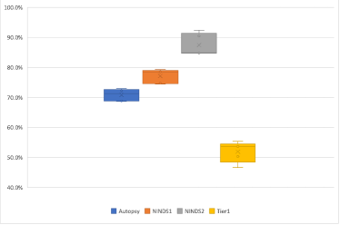
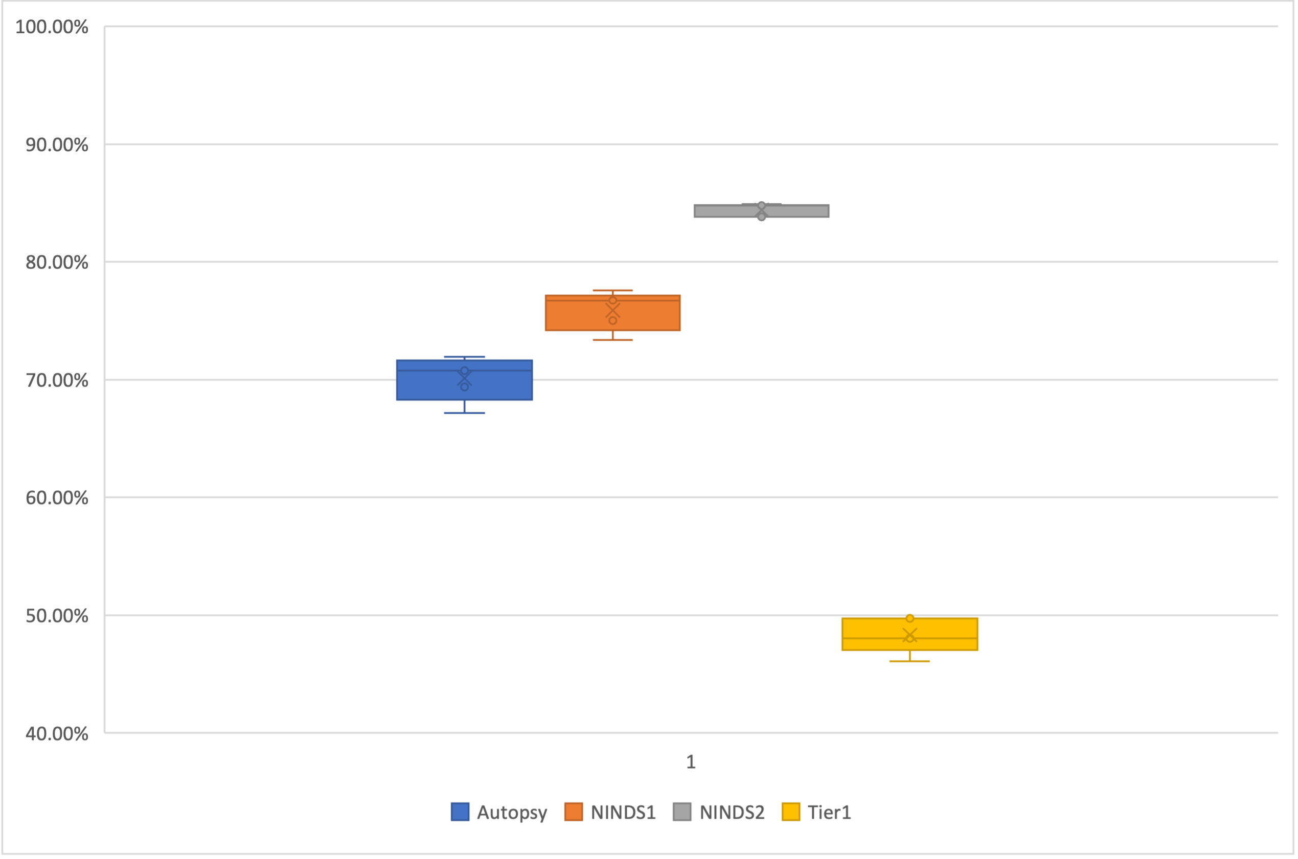
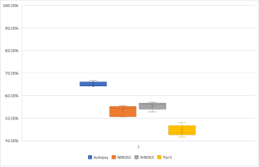
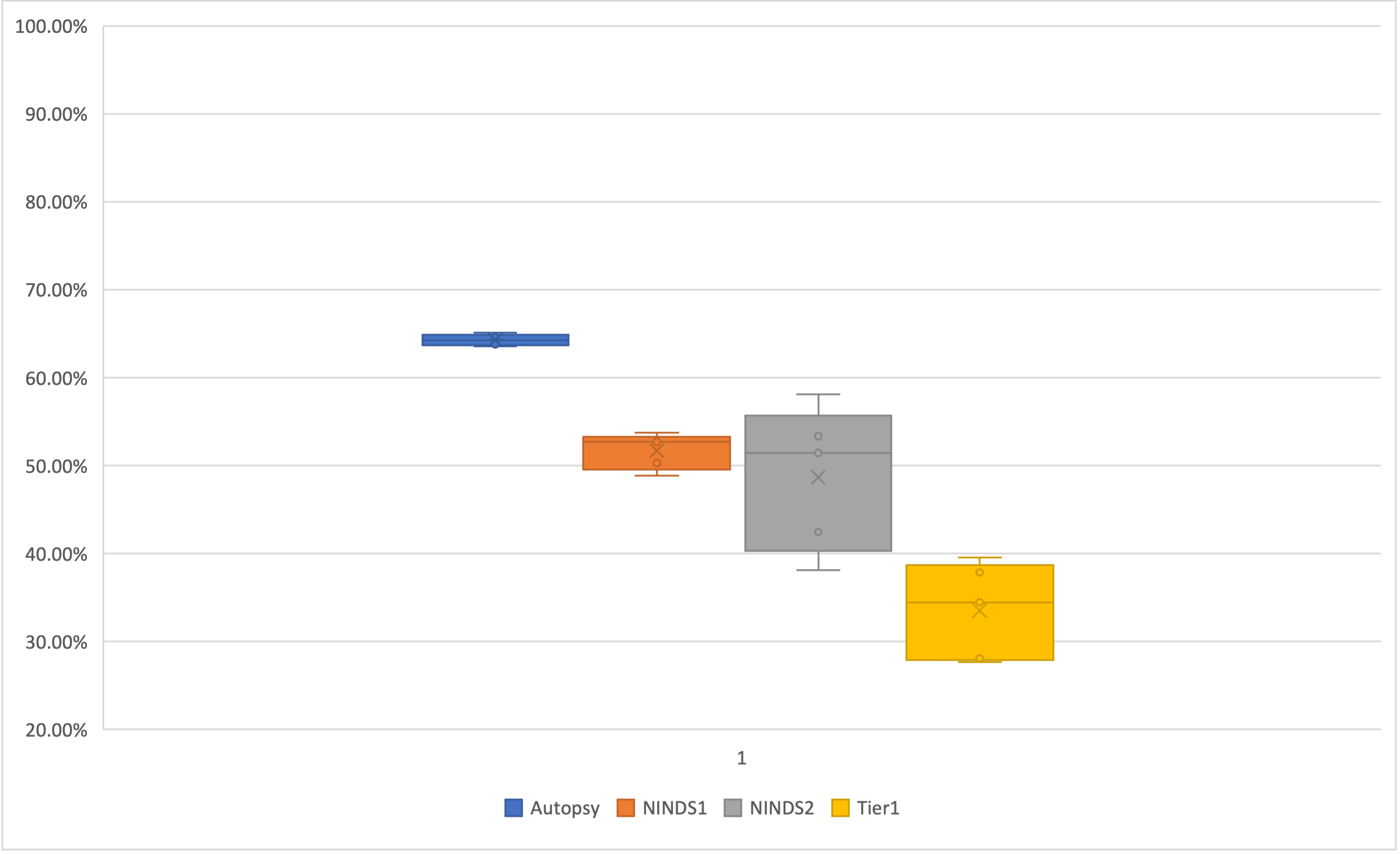
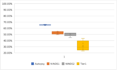
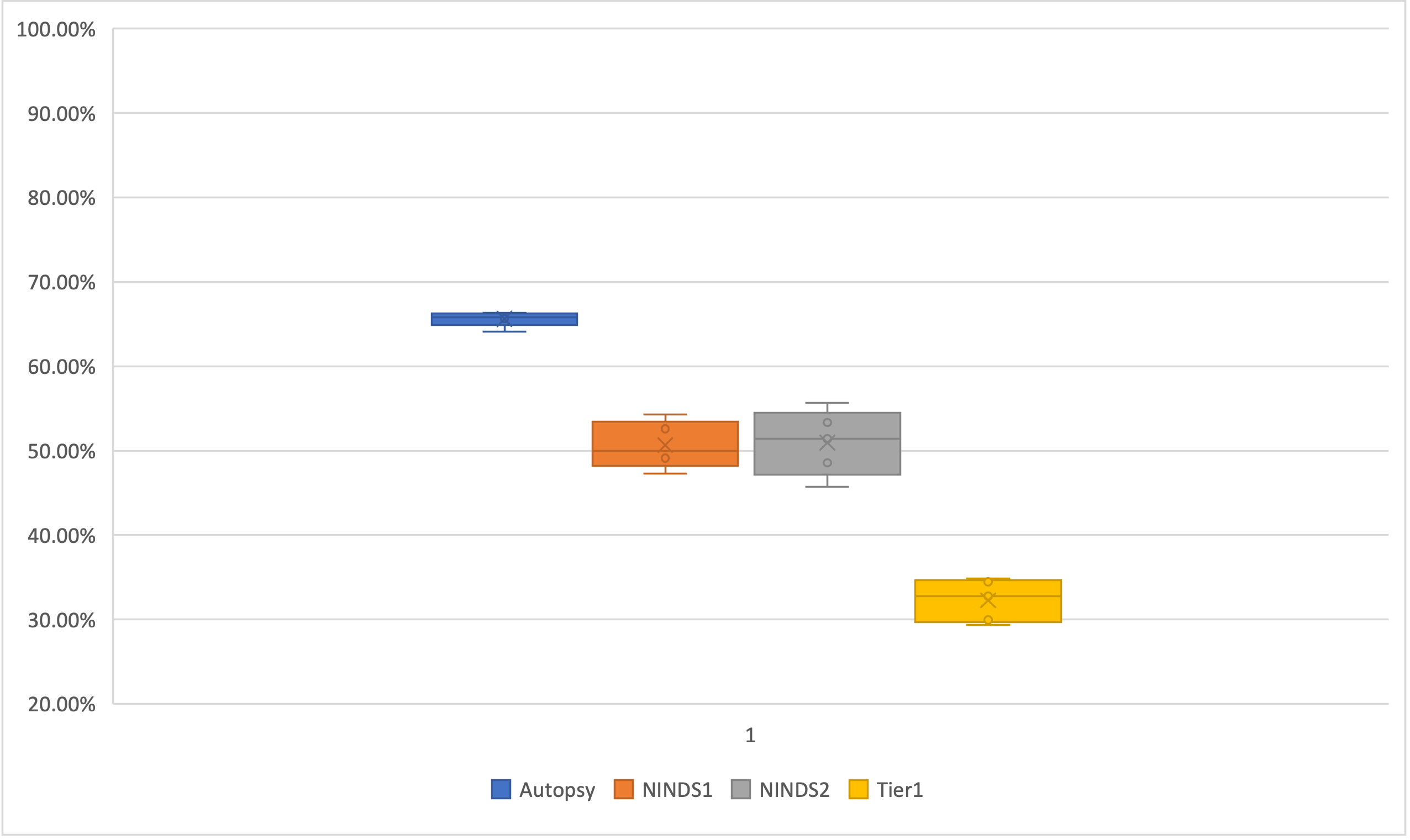
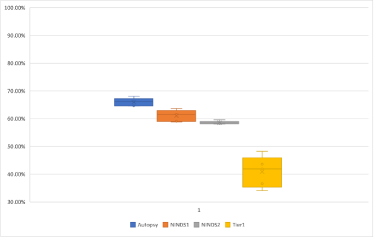
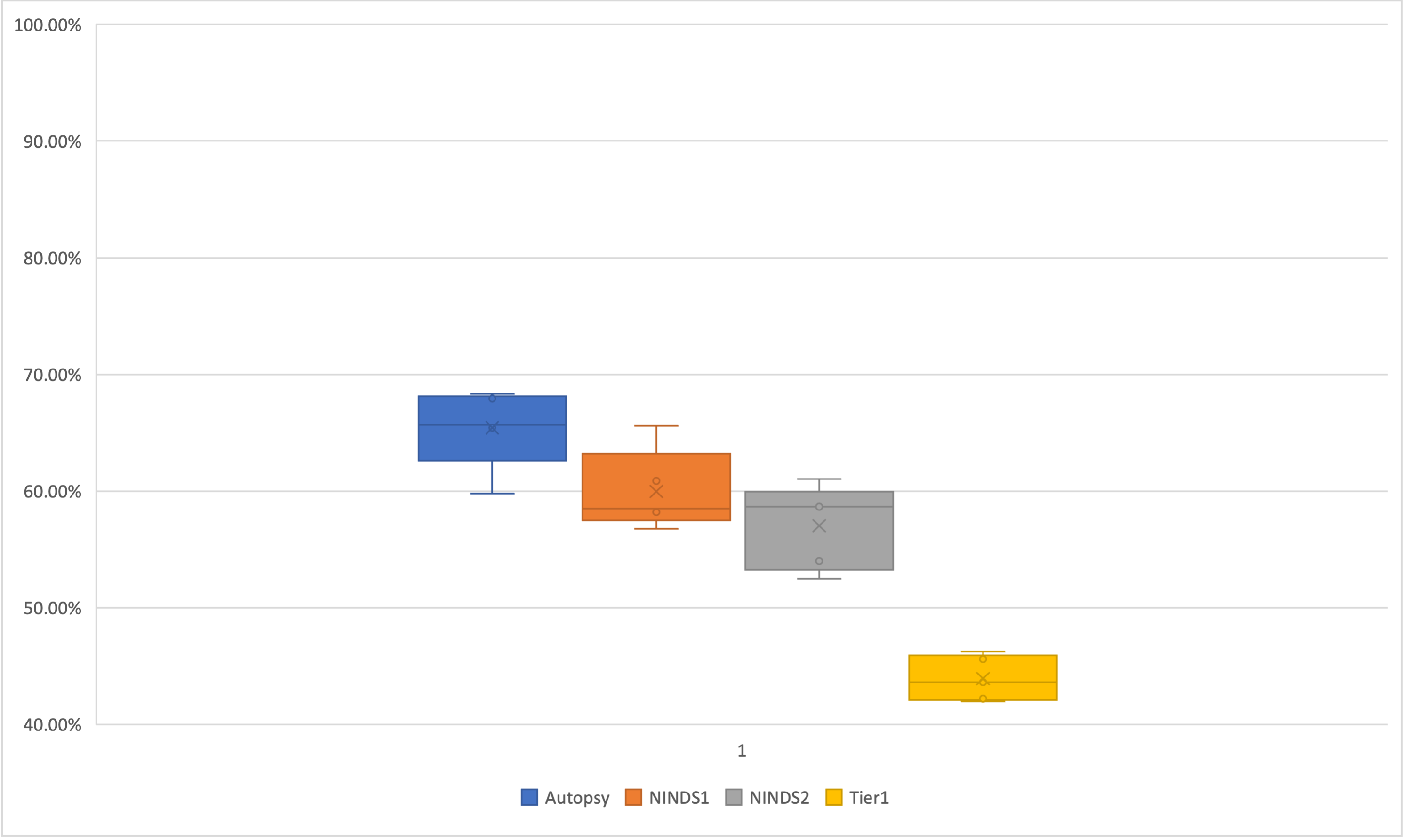
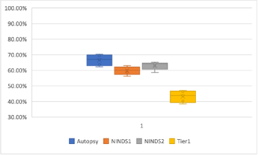
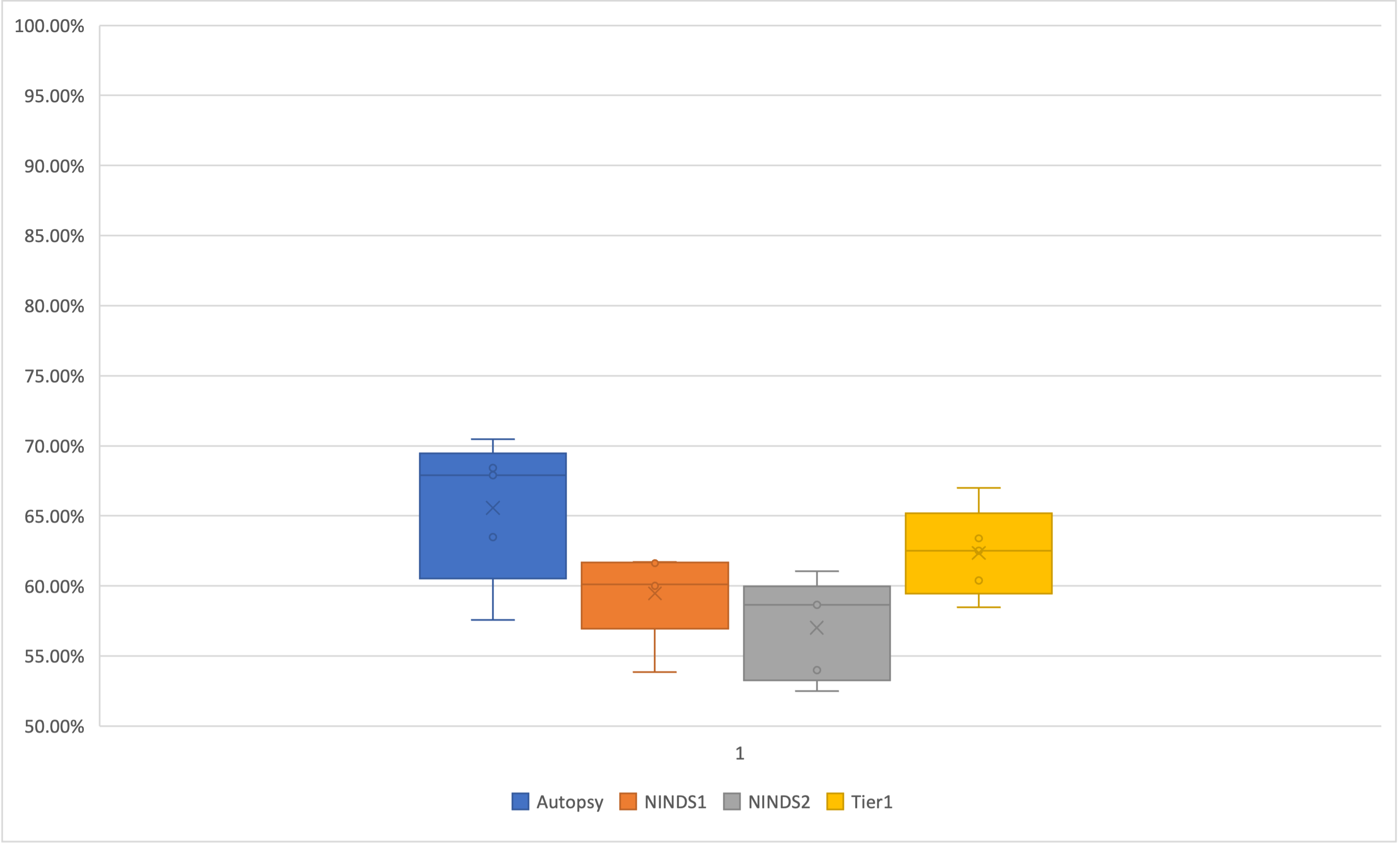
Approach 0 (A) obtained the highest accuracy for all datasets (Table 3 and Figures 1 and 2). We anticipated that Approach 0 would achieve the highest accuracy because there is no technical variation among the samples used. Approaches 1 & 2, and Approaches 3 & 4 have similar accuracy. Approaches 3 & 4 achieved higher accuracy than approaches 1 & 2 on Autopsy, NINDS1, and NINDS2. This lead us to recommend to perform feature selection on merged datasets. As extending the list of most common SNPs with SNPs in LD with the most common SNPs (mode B) did not improve accuracy, for the following analyses we considered only the SNPs obtained using mode A.
| Approach | ||||
| Approach 0 (A) | ||||
| Approach 1 (A) | ||||
| Approach 2 (A) | ||||
| Approach 3 (A) | ||||
| Approach 4 (A) | ||||
| Approach 0 (B) | ||||
| Approach 1 (B) | ||||
| Approach 2 (B) | ||||
| Approach 3 (B) | ||||
| Approach 4 (B) |
In Figure 3, we show the number of SNPs and genes that are in common among different integration approaches for the same dataset. To get the genes where the SNPs are located we used the Biomart platform [54]. On average around 6% of the SNPs identified using Approach 0 (without data integration) are replicated by at least one other approach (Supplementary Figures), while on average % of the SNPs identified with any data integration strategy (Approaches 1 to 4) are replicated by at least one other integration approach (Figure 3). This indicates that integrating datasets increases by six-fold the proportion of replicated SNPs. The highest agreement was observed between Approaches 3 and 4, followed by Approaches 1 and 2. Figure 3(f) only includes three approaches because there were no common SNPs between Approach 1 and Approaches 2, 3, and 4.

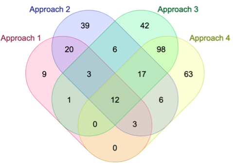
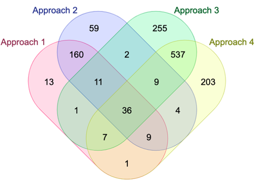
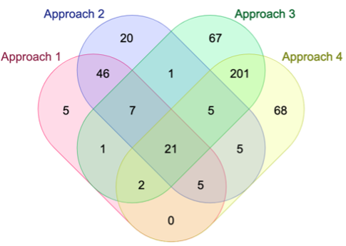


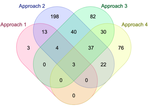

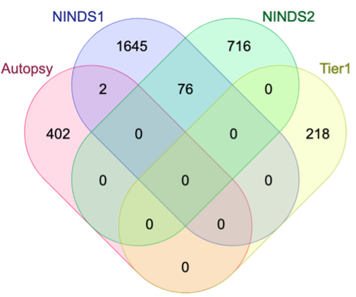
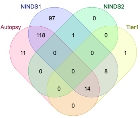
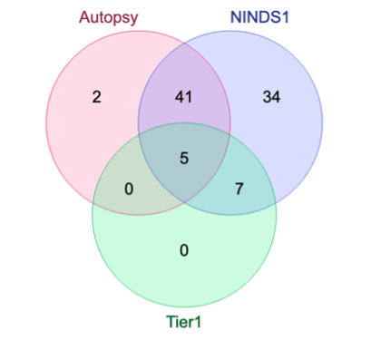
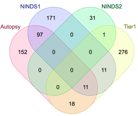
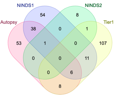
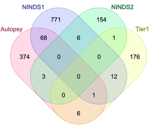
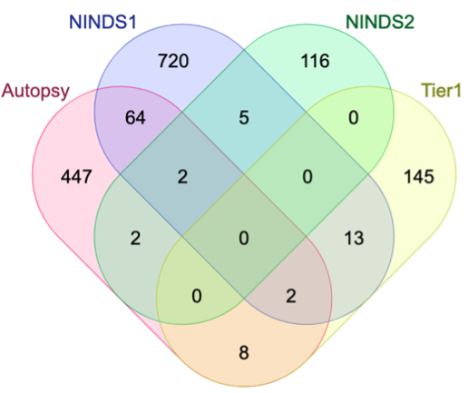
Figure 4 shows the number of identified SNPs and genes that are in agreement using different datasets per approach. The number of SNPs in agreement between datasets fell dramatically when using different datasets but the same approach. The highest pair-wise agreement is in Approach 0 between NINDS1 and NINDS2 which are two datasets generated by the same studies. This suggests that the genotyping platform and study design are the greatest source of variation. If we consider NINDS1 and NINDS2 as the same dataset then the number of genes reproduced by at least two different datasets goes from 33 in Approach 0 to 75 in Approach 4. This suggests that integrating datasets more than duplicates the number of genes that are reproduced in at least two datasets.


3.1 Phenotypes associated with potential biomarkers
To investigate whether SNPs identified by at least two datasets or two approaches (referred to as replicated SNPs) are associated with PD, we retrieved the phenotype associated with each of these replicated SNPs using the Biomart platform. Four of these replicated SNPs (rs11248060, rs239748, rs999473, and rs2313982) are directly linked to PD. By performing a literature search on the associated phenotypes, we found 50 other replicated SNPs indirectly associated with PD. That is, they are directly associated with a disease that frequently co-occurs with PD. These 50 replicated SNPs together with the manuscripts used as basis of their indirect association to PD are listed in Supplementary File 1. These 50 replicated SNPs open up new potential avenues of investigation for PD biomarkers.
4 Conclusion
The integration of datasets may result in a slight decrease in classification accuracy but it can significantly enhance the reproducibility of potential biomarkers. We show that on average 93% of the SNPs discovered using a single data set are not replicated in other datasets, and that dataset integration reduces that average lack of replication to 62%. A limitation of this study is that SNPs genotyped on each dataset differ due to different genotyping platforms, leading to the exclusion of many SNPs as potential biomarkers when integrating data sets. To address this issue, repeating the study on SNPs detected by whole-genome sequencing could be a solution. In addition, accessing other datasets from diverse populations would enable us to further test the replication of our identified SNPs. Moreover, our methodology is applicable to various diseases such as breast cancer, lung cancer, and colorectal cancer.
Declaration of Interest
None.
Funding Sources
This research was partially supported by grants from the Natural Sciences and Engineering Research Council of Canada (NSERC) to L.P.-C. and H.U. A.A was partially supported by funding from Memorial University School of Graduate Studies.
Declaration of generative AI in scientific writing
During the preparation of this work the author(s) used Grammarly and ChatGPT in order to check the grammar and improve clarity. After using this tool/service, the author(s) reviewed and edited the content as needed and take(s) full responsibility for the content of the publication.
References
- [1] J. Jankovic, Parkinson’s disease: clinical features and diagnosis, Journal of Neurology, Neurosurgery, & Psychiatry 79 (4) (2008) 368–376.
- [2] J. Contreras-Vidal, G. E. Stelmach, Effects of Parkinsonism on motor control, Life Sciences 58 (3) (1995) 165–176.
- [3] American Association of Neurological Surgeons, https://www.aans.org/en/Patients/Neurosurgical-Conditions-and-Treatments/Parkinsons-Disease, accessed: October 2022.
- [4] J. Opara, W. Brola, M. Leonardi, B. Błaszczyk, Quality of life in Parkinsons disease, Journal of Medicine and Life 5 (4) (2012) 375.
- [5] S. J. Johnson, M. D. Diener, A. Kaltenboeck, H. G. Birnbaum, A. D. Siderowf, An economic model of Parkinson’s disease: Implications for slowing progression in the United States, Movement Disorders 28 (3) (2013) 319–326.
- [6] S. L. Kowal, T. M. Dall, R. Chakrabarti, M. V. Storm, A. Jain, The current and projected economic burden of Parkinson’s disease in the United States, Movement Disorders 28 (3) (2013) 311–318.
- [7] J.-X. Yang, L. Chen, Economic burden analysis of Parkinson’s disease patients in China, Parkinson’s Disease 2017 (2017).
- [8] O.-B. Tysnes, A. Storstein, Epidemiology of Parkinson’s disease, Journal of Neural Transmission 124 (8) (2017) 901–905.
- [9] E. R. Dorsey, A. Elbaz, E. Nichols, N. Abbasi, F. Abd-Allah, A. Abdelalim, J. C. Adsuar, M. G. Ansha, C. Brayne, J.-Y. J. Choi, et al., Global, regional, and national burden of Parkinson’s disease, 1990–2016: a systematic analysis for the Global Burden of Disease Study 2016, The Lancet Neurology 17 (11) (2018) 939–953.
- [10] C. Tremblay, P. D. Martel, J. Frasnelli, Trigeminal system in Parkinson’s disease: A potential avenue to detect Parkinson-specific olfactory dysfunction, Parkinsonism & Related Disorders 44 (2017) 85–90.
- [11] T. A. Zesiewicz, K. L. Sullivan, R. A. Hauser, Nonmotor symptoms of Parkinson’s disease, Expert Review of Neurotherapeutics 6 (12) (2006) 1811–1822.
- [12] H. Braak, K. Del Tredici, U. Rüb, R. A. De Vos, E. N. J. Steur, E. Braak, Staging of brain pathology related to sporadic Parkinson’s disease, Neurobiology of Aging 24 (2) (2003) 197–211.
- [13] R. B. Postuma, D. Berg, M. Stern, W. Poewe, C. W. Olanow, W. Oertel, J. Obeso, K. Marek, I. Litvan, A. E. Lang, et al., MDS clinical diagnostic criteria for Parkinson’s disease, Movement Disorders 30 (12) (2015) 1591–1601.
- [14] P. Drotár, J. Mekyska, I. Rektorová, L. Masarová, Z. Smékal, M. Faundez-Zanuy, Decision support framework for Parkinson’s disease based on novel handwriting markers, IEEE Transactions on Neural Systems and Rehabilitation Engineering 23 (3) (2014) 508–516.
- [15] C. R. Pereira, D. R. Pereira, G. H. Rosa, V. H. Albuquerque, S. A. Weber, C. Hook, J. P. Papa, Handwritten dynamics assessment through convolutional neural networks: An application to Parkinson’s disease identification, Artificial Intelligence in Medicine 87 (2018) 67–77.
- [16] A. Li, C. Li, Detecting Parkinson’s disease through gait measures using machine learning, Diagnostics 12 (10) (2022) 2404.
- [17] F. Wahid, R. K. Begg, C. J. Hass, S. Halgamuge, D. C. Ackland, Classification of Parkinson’s disease gait using spatial-temporal gait features, IEEE Journal of Biomedical and Health Informatics 19 (6) (2015) 1794–1802.
- [18] T. D. Pham, H. Yan, Tensor decomposition of gait dynamics in Parkinson’s disease, IEEE Transactions on Biomedical Engineering 65 (8) (2017) 1820–1827.
- [19] A. Cherubini, M. Morelli, R. Nisticó, M. Salsone, G. Arabia, R. Vasta, A. Augimeri, M. E. Caligiuri, A. Quattrone, Magnetic resonance support vector machine discriminates between Parkinson’s disease and progressive supranuclear palsy, Movement Disorders 29 (2) (2014) 266–269.
- [20] H. Choi, S. Ha, H. J. Im, S. H. Paek, D. S. Lee, Refining diagnosis of Parkinson’s disease with deep learning-based interpretation of dopamine transporter imaging, NeuroImage: Clinical 16 (2017) 586–594.
- [21] F. Segovia, J. M. Gorriz, J. Ramirez, F. J. Martinez-Murcia, D. Castillo-Barnes, Assisted diagnosis of Parkinsonism based on the striatal morphology, International Journal of Neural Systems 29 (09) (2019) 1950011.
- [22] B. E. Sakar, M. E. Isenkul, C. O. Sakar, A. Sertbas, F. Gurgen, S. Delil, H. Apaydin, O. Kursun, Collection and analysis of a Parkinson speech dataset with multiple types of sound recordings, IEEE Journal of Biomedical and Health Informatics 17 (4) (2013) 828–834.
- [23] C. Ma, J. Ouyang, H.-L. Chen, X.-H. Zhao, An efficient diagnosis system for Parkinson’s disease using kernel-based extreme learning machine with subtractive clustering features weighting approach, Computational and Mathematical Methods in Medicine 2014 (2014).
- [24] P. A. LeWitt, J. Li, M. Lu, T. G. Beach, C. H. Adler, L. Guo, A. Parkinson’s Disease Consortium, 3-hydroxykynurenine and other Parkinson’s disease biomarkers discovered by metabolomic analysis, Movement Disorders 28 (12) (2013) 1653–1660.
- [25] F. Maass, B. Michalke, D. Willkommen, A. Leha, C. Schulte, L. Tönges, B. Mollenhauer, C. Trenkwalder, D. Rückamp, M. Börger, et al., Elemental fingerprint: Reassessment of a cerebrospinal fluid biomarker for Parkinson’s disease, Neurobiology of Disease 134 (2020) 104677.
- [26] S. Nuvoli, A. Spanu, M. L. Fravolini, F. Bianconi, S. Cascianelli, G. Madeddu, B. Palumbo, [123I] Metaiodobenzylguanidine (MIBG) cardiac scintigraphy and automated classification techniques in Parkinsonian disorders, Molecular Imaging and Biology 22 (3) (2020) 703–710.
- [27] C. Váradi, K. Nehéz, O. Hornyák, B. Viskolcz, J. Bones, Serum n-glycosylation in Parkinson’s disease: a novel approach for potential alterations, Molecules 24 (12) (2019) 2220.
- [28] C. Su, J. Tong, F. Wang, Mining genetic and transcriptomic data using machine learning approaches in Parkinson’s disease, npj Parkinson’s Disease 6 (1) (2020) 1–10.
- [29] A. Nunes, G. Silva, C. Duque, C. Januário, I. Santana, A. F. Ambrósio, M. Castelo-Branco, R. Bernardes, Retinal texture biomarkers may help to discriminate between Alzheimer, Parkinson, and healthy controls, PlOS One 14 (6) (2019) e0218826.
- [30] Z. Wang, X. Zhu, E. Adeli, Y. Zhu, F. Nie, B. Munsell, G. Wu, et al., Multi-modal classification of neurodegenerative disease by progressive graph-based transductive learning, Medical Image Analysis 39 (2017) 218–230.
- [31] M. Afshar, H. Usefi, Dimensionality reduction using singular vectors, Scientific Reports 11 (1) (2021) 1–13.
- [32] L. Breiman, Random forests, Machine Learning 45 (1) (2001) 5–32.
- [33] National Library of Medicine. The ncbi dbGaP database of genotypes and phenotypes [online]. Accessed: September 2022.
- [34] U. Johns Hopkins University Center for Inherited Disease Research (CIDR). Baltimore, MD, CIDR: Genome Wide Association Study in Familial Parkinson’s disease (PD), https://www.ncbi.nlm.nih.gov/projects/gap/cgi-bin/study.cgi?study_id=phs000126.v2.p1 (2016).
- [35] W. Nichols, V. Elsaesser, N. Pankratz, M. Pauciulo, D. Marek, C. Halter, A. Rudolph, C. Shults, T. Foroud, et al., LRRK2 mutation analysis in Parkinson’s disease families with evidence of linkage to PARK8, Neurology 69 (18) (2007) 1737–1744.
- [36] N. Pankratz, M. W. Pauciulo, V. E. Elsaesser, D. K. Marek, C. A. Halter, A. Rudolph, C. W. Shults, T. Foroud, W. C. Nichols, Mutations in LRRK2 other than G2019S are rare in a north american–based sample of familial Parkinson’s disease, Movement Disorders: Official Journal of the Movement Disorder Society 21 (12) (2006) 2257–2260.
- [37] W. C. Nichols, N. Pankratz, D. Hernandez, C. Paisán-Ruíz, S. Jain, C. A. Halter, V. E. Michaels, T. Reed, A. Rudolph, C. W. Shults, et al., Genetic screening for a single common LRRK2 mutation in familial Parkinson’s disease, The Lancet 365 (9457) (2005) 410–412.
- [38] J. Wilk, J. Tobin, O. Suchowersky, H. A. Shill, C. Klein, G. Wooten, M. Lew, M. Mark, M. Guttman, R. Watts, et al., Herbicide exposure modifies GSTP1 haplotype association to Parkinson onset age: the GenePD Study, Neurology 67 (12) (2006) 2206–2210.
- [39] M. Sun, J. C. Latourelle, G. F. Wooten, M. F. Lew, C. Klein, H. A. Shill, L. I. Golbe, M. H. Mark, B. A. Racette, J. S. Perlmutter, et al., Influence of heterozygosity for parkin mutation on onset age in familial Parkinson disease: the GenePD Study, Archives of Neurology 63 (6) (2006) 826–832.
- [40] S. Karamohamed, J. Latourelle, B. Racette, J. Perlmutter, G. Wooten, M. Lew, C. Klein, H. Shill, L. Golbe, M. Mark, et al., BDNF genetic variants are associated with onset age of familial Parkinson disease: GenePD Study, Neurology 65 (11) (2005) 1823–1825.
- [41] S. Karamohamed, L. Golbe, M. Mark, A. Lazzarini, O. Suchowersky, N. Labelle, M. Guttman, L. Currie, G. Wooten, M. Stacy, et al., Absence of previously reported variants in the SCNA (G88C and G209A), NR4A2 (T291D and T245G) and the DJ-1 (T497C) genes in familial Parkinson’s disease from the GenePD Study, Movement Disorders: Official Journal of the Movement Disorder Society 20 (9) (2005) 1188–1191.
- [42] U. Johns Hopkins University Center for Inherited Disease Research (CIDR). Baltimore, MD, Autopsy-confirmed Parkinson disease GWAS consortium (APDGC), https://www.ncbi.nlm.nih.gov/projects/gap/cgi-bin/study.cgi?study_id=phs000394.v1.p1 (2012).
- [43] D. Andrew Singleton, National Institute of Neurological Disorders and Stroke (NINDS) Genome-wide genotyping in Parkinson’s disease, https://www.ncbi.nlm.nih.gov/projects/gap/cgi-bin/study.cgi?study_id=phs000089.v4.p2, accessed: September 2022.
- [44] H.-C. Fung, S. Scholz, M. Matarin, J. Simón-Sánchez, D. Hernandez, A. Britton, J. R. Gibbs, C. Langefeld, M. L. Stiegert, J. Schymick, et al., Genome-wide genotyping in Parkinson’s disease and neurologically normal controls: first stage analysis and public release of data, The Lancet Neurology 5 (11) (2006) 911–916.
- [45] J. Simon-Sanchez, S. Scholz, H.-C. Fung, M. Matarin, D. Hernandez, J. R. Gibbs, A. Britton, F. W. de Vrieze, E. Peckham, K. Gwinn-Hardy, et al., Genome-wide SNP assay reveals structural genomic variation, extended homozygosity and cell-line induced alterations in normal individuals, Human Molecular Genetics 16 (1) (2007) 1–14.
- [46] J. Simon-Sanchez, C. Schulte, J. M. Bras, M. Sharma, J. R. Gibbs, D. Berg, C. Paisan-Ruiz, P. Lichtner, S. W. Scholz, D. G. Hernandez, et al., Genome-wide association study reveals genetic risk underlying Parkinson’s disease, Nature Genetics 41 (12) (2009) 1308–1312.
- [47] J. M. Sanz, S. Falzoni, M. L. Morieri, A. Passaro, G. Zuliani, F. Di Virgilio, Association of hypomorphic P2X7 receptor genotype with age, Frontiers in Molecular Neuroscience 13 (2020) 8.
- [48] Demetrius Maraganore. Mayo Clinic Rochester MN USA, Mayo-perlegen LEAPS (linked efforts to accelerate Parkinson's solutions) collaboration, https://www.ncbi.nlm.nih.gov/projects/gap/cgi-bin/study.cgi?study_id=phs000048.v1.p1, accessed: September 2022.
- [49] D. M. Maraganore, M. De Andrade, T. G. Lesnick, K. J. Strain, M. J. Farrer, W. A. Rocca, P. K. Pant, K. A. Frazer, D. R. Cox, D. G. Ballinger, High-resolution whole-genome association study of Parkinson’s disease, The American Journal of Human Genetics 77 (5) (2005) 685–693.
- [50] E. Evangelou, D. M. Maraganore, J. P. Ioannidis, Meta-analysis in genome-wide association datasets: strategies and application in Parkinson’s disease, PLOS One 2 (2) (2007) e196.
- [51] T. G. Lesnick, S. Papapetropoulos, D. C. Mash, J. Ffrench-Mullen, L. Shehadeh, M. De Andrade, J. R. Henley, W. A. Rocca, J. E. Ahlskog, D. M. Maraganore, A genomic pathway approach to a complex disease: axon guidance and Parkinson’s disease, PLOS Genetics 3 (6) (2007) e98.
- [52] H. Schwender, Imputing missing genotypes with weighted k nearest neighbors, Journal of Toxicology and Environmental Health, Part A 75 (8-10) (2012) 438–446.
- [53] M. Arnold, J. Raffler, A. Pfeufer, K. Suhre, G. Kastenmüller, SNiPA: an interactive, genetic variant-centered annotation browser, Bioinformatics 31 (8) (2015) 1334–1336.
- [54] Ensemble, Ensemble Biomart, http://useast.ensembl.org/biomart/martview/fbd18081f77c6d6aa53ba6f63544988b (2022).