Quantized vortex dynamics of the nonlinear Schrödinger equation on torus with non-vanishing momentum

Abstract

We derive rigorously the reduced dynamical law for quantized vortex dynamics of the nonlinear Schrödinger equation on the torus with non-vanishing momentum when the vortex core size $\varepsilon\to 0$. The reduced dynamical law is governed by a Hamiltonian flow driven by a renormalized energy. A key ingredient is to construct a new canonical harmonic map to include the effect from the non-vanishing momentum into the dynamics. Finally, some properties of the reduced dynamical law are discussed.

1 Introduction

In this paper, we study quantized vortex dynamics of the nonlinear Schrödinger equation (NLSE) on the torus [10, 27]:

$$i\partial_{t}u^{\varepsilon}(\boldsymbol{x},t)-\Delta u^{\varepsilon}(\boldsymbol{x},t)+\frac{1}{\varepsilon^{2}}\left(|u^{\varepsilon}(\boldsymbol{x},t)|^{2}-1\right)u^{\varepsilon}(\boldsymbol{x},t)=0,\quad\boldsymbol{x}\in\mathbb{T}^{2},\ t>0,$$ (1.1)

with initial data

$$u^{\varepsilon}(\boldsymbol{x},0)=u_{0}^{\varepsilon}(\boldsymbol{x}),\quad\boldsymbol{x}\in\mathbb{T}^{2},$$ (1.2)

where $t$ is the time variable, $\mathbb{T}^{2}=(\mathbb{R}/\mathbb{Z})\times(\mathbb{R}/\mathbb{Z})$ is the unit torus, $\boldsymbol{x}=(x,y)^{T}$ is the spatial coordinate, $u^{\varepsilon}:=u^{\varepsilon}(\boldsymbol{x},t)$ is a complex-valued wave function or order parameter, $0<\varepsilon<<1$ is a dimensionless parameter which is used to characterize the core size of quantized vortices, and $u_{0}^{\varepsilon}:=u_{0}^{\varepsilon}(\boldsymbol{x})$ is a given initial data. It is well-known that the NLSE (1.1) conserves the mass defined as [22]

$$M(u^{\varepsilon}(t)):=\int_{\mathbb{T}^{2}}|u^{\varepsilon}(\boldsymbol{x},t)|^{2}d\boldsymbol{x}\equiv\int_{\mathbb{T}^{2}}|u^{\varepsilon}_{0}(\boldsymbol{x})|^{2}d\boldsymbol{x}:=M(u^{\varepsilon}_{0}),\qquad t\geq 0;$$ (1.3)

the momentum defined as [10, 14, 22]

$$\boldsymbol{Q}(u^{\varepsilon}(t)):=\int_{\mathbb{T}^{2}}\boldsymbol{j}(u^{\varepsilon}(\boldsymbol{x},t))d\boldsymbol{x}\equiv\int_{\mathbb{T}^{2}}\boldsymbol{j}(u^{\varepsilon}_{0}(\boldsymbol{x}))d\boldsymbol{x}=\boldsymbol{Q}(u^{\varepsilon}_{0}):=\boldsymbol{Q}_{0}^{\varepsilon}\qquad t\geq 0;$$ (1.4)

and the energy defined as [10, 14, 22]

$$E(u^{\varepsilon}(t)):=\int_{\mathbb{T}^{2}}e(u^{\varepsilon}(\boldsymbol{x},t))d\boldsymbol{x}\equiv\int_{\mathbb{T}^{2}}e(u^{\varepsilon}_{0}(\boldsymbol{x}))d\boldsymbol{x}=E(u^{\varepsilon}_{0}),\quad t\geq 0.$$ (1.5)

Here we adopt the notations, for any complex-valued function $v(\boldsymbol{x}):\ \mathbb{T}^{2}\to{\mathbb{C}}$, its corresponding current $\boldsymbol{j}(v)$, energy density $e(v)$ and Jacobian $J(v)$ are defined as

$$\boldsymbol{j}(v):=\mathrm{Im}\,(\overline{v}\nabla v),\quad e(v):=\frac{1}{2}|\nabla v|^{2}+\frac{1}{4\varepsilon^{2}}(1-|v|^{2})^{2},\quad J(v)=\frac{1}{2}\nabla\cdot(\mathbb{J}\boldsymbol{j}(v))=\mathrm{Im}\,(\partial_{x}\overline{v}\,\partial_{y}v),$$ (1.6)

where $\overline{v}$ and $\mathrm{Im}\,(v)$ denote the complex conjugate and imaginary part of the function $v$, respectively, and $\mathbb{J}$ is a symplectic matrix given as

$$\mathbb{J}=\left(\begin{array}[]{cc}0&1\\ -1&0\end{array}\right).$$

The NLSE (1.1), also known as the Gross-Pitaevskii equation (GPE) [28, 1], has been widely used as a phenomenological model for superfluidity, such as liquid helium [26, 17, 22] and Bose-Einstein condensation [1]. A key signature of superfluidity is the appearance of quantized vortices which are particle-like or topological defects. Quantized vortices in two dimensions are those particle-like defects whose centers are zeros of the order parameter or wave function, possessing localized phase singularity with the topological charge (also known as winding number, index, or circulation) being quantized. They have been widely observed in many different physical systems, such as liquid Helium, atomic gases, nonlinear optics and type-II superconductors [26, 8, 2]. Their study remains one of the most important and fundamental problems since they were predicted by Lars Onsager in 1947 in connection with superfluid Helium.

Several analytical and numerical studies have dealt with quantized vortex states of the NLSE (1.1) and their interactions as well as the reduced dynamical laws of quantized vortex lattice when $\varepsilon\to 0$ [3, 25, 29]. For results in the whole space ${\mathbb{R}}^{2}$ or on bounded domains with either Dirichlet or homogeneous Neumann boundary conditions, we refer to [7, 10, 14, 19, 22, 28, 12, 13, 18, 20, 21, 15, 16, 4, 5] and references therein. Based on mathematical analysis and numerical simulation results [24, 25, 23], for a quantized vortex with winding number $m$, when $m=\pm 1$, it is dynamically (or structurally) stable; and when $|m|>1$, it is unstable.

For the NLSE (1.1) on the torus, due to the periodic-type boundary condition, there can exist several isolated and distinct quantized vortices in the initial data $u_{0}^{\varepsilon}:=u_{0}^{\varepsilon}(\boldsymbol{x})$, while the winding number of each quantized vortex is either $+1$ or $-1$ [10]. It is well-known in the literature that the total number of quantized vortices in the initial data has to be an even integer and half of them with winding number $+1$ and the other half of them with winding number $-1$ [10]. We assume that in $u_{0}^{\varepsilon}$ there are $2N(N\in{\mathbb{N}})$ isolated and distinct quantized vortices whose centers are located at $\boldsymbol{a}^{0,\varepsilon}_{1},\boldsymbol{a}^{0,\varepsilon}_{2},\ldots,\boldsymbol{a}^{0,\varepsilon}_{2N}\in\mathbb{T}^{2}$ with winding number $d_{1},d_{2},\ldots,d_{2N}\in\{\pm 1\}$, respectively. Without loss of generality, we assume

$$d_{1}=\ldots=d_{N}=1,\ d_{N+1}=\ldots=d_{2N}=-1,\quad\boldsymbol{a}^{0,\varepsilon}_{j}\neq\boldsymbol{a}^{0,\varepsilon}_{k},\ 1\leq j\neq k\leq 2N.\qquad$$ (1.7)

Assume

$$\boldsymbol{a}^{0}_{j}:=\lim_{\varepsilon\to 0}\boldsymbol{a}^{0,\varepsilon}_{j},\quad 1\leq j\leq 2N.$$ (1.8)

Then one has

$$\boldsymbol{Q}_{0}:=\lim_{\varepsilon\to 0}\boldsymbol{Q}(u^{\varepsilon}_{0})=2\pi\mathbb{J}\sum_{j=1}^{2N}d_{j}\boldsymbol{a}^{0}_{j}=2\pi\mathbb{J}\left[\sum_{j=1}^{N}\boldsymbol{a}^{0}_{j}-\sum_{j=1}^{N}\boldsymbol{a}^{0}_{N+j}\right].$$ (1.9)

Under the assumption of the vanishing momentum of the initial data, i.e.

$$\boldsymbol{a}^{0}_{j}\neq\boldsymbol{a}^{0}_{k},\quad 1\leq j\neq k\leq 2N,\qquad\boldsymbol{Q}_{0}=\lim_{\varepsilon\to 0}\boldsymbol{Q}_{0}^{\varepsilon}={\bf 0}\in{\mathbb{R}}^{2},$$ (1.10)

and

$$J(u^{\varepsilon}_{0})\stackrel{{\scriptstyle\varepsilon\to 0^{+}}}{{\longrightarrow}}\pi\sum_{j=1}^{2N}d_{j}\delta_{\boldsymbol{a}^{0}_{j}}\ \text{in}\ W^{-1,1}(\mathbb{T}^{2}):=[W^{1,\infty}(\mathbb{T}^{2})]^{\prime},$$ (1.11)

with $\delta(\boldsymbol{x})$ the Dirac delta function and $\delta_{\boldsymbol{a}^{0}_{j}}:=\delta_{\boldsymbol{a}^{0}_{j}}(\boldsymbol{x})$ defined as $\delta_{\boldsymbol{a}^{0}_{j}}(\boldsymbol{x})=\delta(\boldsymbol{x}-\boldsymbol{a}^{0}_{j})$ for $1\leq j\leq 2N$, Colliander and Jerrard [10] established the reduced dynamical law of quantized vortex of the NLSE (1.1) with (1.2) when $\varepsilon\to 0$: for $t\geq 0$, there exists the $j$-th vortex path, denoted as $\boldsymbol{a}^{\varepsilon}_{j}(t)$ satisfying $\boldsymbol{a}^{\varepsilon}_{j}(0)=\boldsymbol{a}^{0,\varepsilon}_{j}$, in the solution $u^{\varepsilon}(\boldsymbol{x},t)$ of the NLSE (1.1) originated from $\boldsymbol{a}^{0,\varepsilon}_{j}$, for $j=1,\ldots,2N$. Denote

$$\begin{aligned} &\boldsymbol{a}_{j}:=\boldsymbol{a}_{j}(t):=\lim_{\varepsilon\to 0}\boldsymbol{a}^{\varepsilon}_{j}(t),\quad j=1,\ldots,2N,\\ &\boldsymbol{a}:=\boldsymbol{a}(t)=(\boldsymbol{a}_{1}(t),\ldots,\boldsymbol{a}_{2N}(t))^{T}\in(\mathbb{T}^{2})^{2N}_{*},\end{aligned}\qquad t\geq 0$$ (1.12)

with

$$(\mathbb{T}^{2})^{2N}_{*}:=\left\{(\boldsymbol{a}_{1},\cdots,\boldsymbol{a}_{2N})^{T}\in(\mathbb{T}^{2})^{2N}|\boldsymbol{a}_{k}\neq\boldsymbol{a}_{m}\ \text{for any}\ 1\leq k\neq m\leq 2N\right\}.$$ (1.13)

Then when $\varepsilon\to 0$, $\boldsymbol{a}(t)$ satisfies the following reduced dynamical law:

$$\dot{\boldsymbol{a}}_{j}=-d_{j}\frac{1}{\pi}\mathbb{J}\nabla_{\boldsymbol{a}_{j}}W(\boldsymbol{a})=2\mathbb{J}\sum_{1\leq k\leq 2N,\;k\neq j}d_{k}\,\nabla F(\boldsymbol{a}_{j}-\boldsymbol{a}_{k}),\qquad 1\leq j\leq 2N,$$ (1.14)

with initial data

$$\boldsymbol{a}_{j}(0)=\boldsymbol{a}_{j}^{0},\qquad 1\leq j\leq 2N;$$ (1.15)

where $W(\boldsymbol{a})$ is the renormalized energy defined as

$$W(\boldsymbol{a})=-\pi\sum_{1\leq k\neq m\leq 2N}d_{k}d_{m}\,F(\boldsymbol{a}_{k}-\boldsymbol{a}_{m}),$$ (1.16)

with $F\in C^{\infty}_{loc}(\mathbb{T}^{2}\setminus\{\boldsymbol{0}\})\cap W^{1,1}(\mathbb{T}^{2})$ the solution of

$$\Delta F(\boldsymbol{x})=2\pi(\delta(\boldsymbol{x})-1),\ \boldsymbol{x}\in\mathbb{T}^{2},\quad{\rm with}\quad\int_{\mathbb{T}^{2}}F(\boldsymbol{x})d\boldsymbol{x}=0.$$ (1.17)

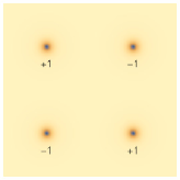
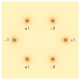
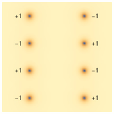
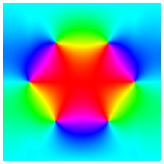
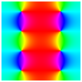
Figure 1: Some typical vanishing momentum initial data $u_{0}^{\varepsilon}:=\sqrt{\rho_{0}^{\varepsilon}}e^{iS_{0}^{\varepsilon}}$: Contour plots of $|u^{\varepsilon}_{0}|$ with vortex center locations with $+1$ and $-1$ as their corresponding winding numbers (top row), and contour plots of the phase function $S_{0}^{\varepsilon}$ (bottom row).

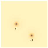
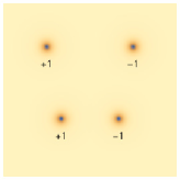
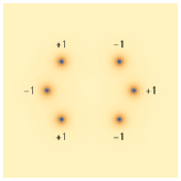
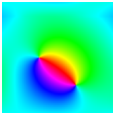
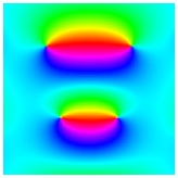
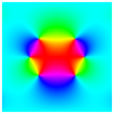
Figure 2: Some typical non-vanishing momentum initial data.

By (1.9), the vanishing momentum assumption used in [10], i.e. $\boldsymbol{Q}_{0}={\bf 0}$, is equivalent to

$$\boldsymbol{0}=\sum_{j=1}^{2N}d_{j}\boldsymbol{a}_{j}^{0}=\sum_{j=1}^{N}\boldsymbol{a}_{j}^{0}-\sum_{j=1}^{N}\boldsymbol{a}_{N+j}^{0}.$$ (1.18)

Thus the vanishing momentum assumption is equivalent to the assumption that the positive mass center is the same as the negative mass center, i.e.

$$\boldsymbol{a}_{+}^{0}=\boldsymbol{a}_{-}^{0},\qquad{\rm with}\qquad\boldsymbol{a}_{+}^{0}:=\frac{1}{N}\sum_{j=1}^{N}\boldsymbol{a}_{j}^{0},\quad\boldsymbol{a}_{-}^{0}:=\frac{1}{N}\sum_{j=N+1}^{2N}\boldsymbol{a}_{j}^{0}.$$ (1.19)

From (1.10) and (1.19), one gets that $N\geq 2$, i.e. $2N\geq 4$, since $\boldsymbol{a}_{+}^{0}\neq\boldsymbol{a}_{-}^{0}$ when $N=1$. In other words, the reduced dynamical law for the NLSE (1.1) obtained in Colliander and Jerrard [10] only works for the case when the initial data $u_{0}^{\varepsilon}$ admits $2N$ ($N\geq 2$, i.e. $4$ or more) vortices with their centers satisfying proper symmetry requirement as stated in (1.19). Clearly, the requirement (1.19) on the initial data $u_{0}^{\varepsilon}$ excludes the non-vanishing momentum initial data, i.e. $\boldsymbol{Q}_{0}=\lim_{\varepsilon\to 0}\boldsymbol{Q}_{0}^{\varepsilon}\neq{\bf 0}$, which includes two different cases: (i) $N=1$, i.e. two vortices; and (ii) $N\geq 2$ and $\boldsymbol{a}_{+}^{0}\neq\boldsymbol{a}_{-}^{0}$. For the convenience of readers, Figure 1 shows some typical initial data with vanishing momentum, while Figure 2 illustrates some typical initial data with non-vanishing momentum.

The main aim of this paper is to extend the reduced dynamical law for quantized vortex dynamics of the NLSE (1.1) with vanishing momentum initial data, i.e. $\boldsymbol{Q}_{0}={\bf 0}$ in (1.8), to non-vanishing momentum initial data, i.e. $\boldsymbol{Q}_{0}\neq{\bf 0}$. A key ingredient is to construct a new canonical harmonic map to include the effect of the non-vanishing momentum into the dynamics. To present our main result, define

$$I(\varepsilon)=\inf_{v\in H^{1}_{g}(B_{1}(\boldsymbol{0}))}\int_{B_{1}(\boldsymbol{0})}\left[\frac{1}{2}|\nabla v|^{2}+\frac{1}{4\varepsilon^{2}}(|v|^{2}-1)^{2}\right]d\boldsymbol{x},$$ (1.20)

where the function space $H^{1}_{g}(B_{1}(\boldsymbol{0}))$ is defined as

$$H_{g}^{1}(B_{1}(\boldsymbol{0}))=\left\{v\in H^{1}(B_{1}(\boldsymbol{0}))\left|v(\boldsymbol{x})=g(\boldsymbol{x})=\frac{x+iy}{|\boldsymbol{x}|}\ \text{for}\ \boldsymbol{x}\in\partial B_{1}(\boldsymbol{0})\right.\right\}.$$

Define

$$\gamma=\lim_{\varepsilon\to 0}\left(I(\varepsilon)-\pi\log\frac{1}{\varepsilon}\right).$$ (1.21)

Introduce a renormalized energy on the torus as [11]

$$W_{\mathbb{T}^{2}}(\boldsymbol{a}) =W(\boldsymbol{a})+2\pi^{2}\left|\sum_{m=1}^{2N}d_{m}\boldsymbol{a}_{m}\right|^{2}$$ (1.22)

$$=-\pi\sum_{1\leq k\neq m\leq 2N}d_{k}d_{m}\,F(\boldsymbol{a}_{k}-\boldsymbol{a}_{m})+2\pi^{2}\left|\sum_{m=1}^{2N}d_{m}\boldsymbol{a}_{m}\right|^{2},\quad\boldsymbol{a}\in(\mathbb{T}^{2})^{2N}_{*},$$

and an $\varepsilon$-dependent renormalized energy as

$$W_{\mathbb{T}^{2}}^{\varepsilon}(\boldsymbol{a}):=2N\left(\pi\log\frac{1}{\varepsilon}+\gamma\right)+W_{\mathbb{T}^{2}}(\boldsymbol{a}),\quad\boldsymbol{a}\in(\mathbb{T}^{2})^{2N}_{*}.$$ (1.23)

Our main result is stated as following:

Theorem 1.1 (Reduced dynamical law for NLSE).

Assume the initial data $u_{0}^{\varepsilon}$ in (1.2) satisfies (1.11) and

$$\lim_{\varepsilon\to 0}\boldsymbol{Q}(u^{\varepsilon}_{0})=\boldsymbol{Q}_{0}:=2\pi\mathbb{J}\left[\sum_{j=1}^{N}\boldsymbol{a}^{0}_{j}-\sum_{j=1}^{N}\boldsymbol{a}^{0}_{N+j}\right],\qquad\limsup_{\varepsilon\to 0}\left[E(u^{\varepsilon}_{0})-W_{\mathbb{T}^{2}}^{\varepsilon}(\boldsymbol{a}^{0})\right]\leq 0.$$ (1.24)

Then there exists a time $T>0$ and $2N$ Lipschitz paths given in (1.12) such that the solution $u^{\varepsilon}$ of the NLSE (1.1) with (1.2) satisfies

$$J(u^{\varepsilon}(t))\stackrel{{\scriptstyle\varepsilon\to 0^{+}}}{{\longrightarrow}}\pi\sum_{j=1}^{2N}d_{j}\delta_{\boldsymbol{a}_{j}(t)}\ \text{in}\ W^{-1,1}(\mathbb{T}^{2}),$$ (1.25)

where $\boldsymbol{a}_{j}(t)$ ($1\leq j\leq 2N$) satisfy the following reduced dynamical law:

$$\dot{\boldsymbol{a}}_{j}=-d_{j}\frac{1}{\pi}\mathbb{J}\nabla_{\boldsymbol{a}_{j}}W(\boldsymbol{a})-2\boldsymbol{Q}_{0}=2\mathbb{J}\sum_{1\leq k\leq 2N,\;k\neq j}d_{k}\,\nabla F(\boldsymbol{a}_{j}-\boldsymbol{a}_{k})-2\boldsymbol{Q}_{0},\quad t>0,$$ (1.26)

with the initial data (1.15).

We remark here that: (i) when $\boldsymbol{Q}_{0}={\bf 0}$, (1.26) collapses to (1.14); and (ii) (1.26) is also equivalent to the following ordinary differential equations (ODEs)

$$\dot{\boldsymbol{a}}_{j}=-d_{j}\frac{1}{\pi}\mathbb{J}\nabla_{\boldsymbol{a}_{j}}W_{\mathbb{T}^{2}}(\boldsymbol{a})=2\mathbb{J}\sum_{1\leq k\leq 2N,\;k\neq j}d_{k}\,\nabla F(\boldsymbol{a}_{j}-\boldsymbol{a}_{k})-4\pi\boldsymbol{q}(\boldsymbol{a}),\quad t>0,$$ (1.27)

where $\boldsymbol{q}(\boldsymbol{a})$ is defined as

$$\boldsymbol{q}(\boldsymbol{a}):=\mathbb{J}\sum_{m=1}^{2N}d_{m}\boldsymbol{a}_{m},\qquad\boldsymbol{a}\in(\mathbb{T}^{2})^{2N}_{*}.$$ (1.28)

Since $\boldsymbol{q}(\boldsymbol{a})$ is a first integral of (1.27), and if $\boldsymbol{a}$ is the solution of (1.27) with the initial data (1.15), we have

$$\boldsymbol{q}(\boldsymbol{a}(t))\equiv\boldsymbol{q}(\boldsymbol{a}(0))=\mathbb{J}\sum_{m=1}^{2N}d_{m}\boldsymbol{a}_{m}^{0}=\frac{1}{2\pi}\boldsymbol{Q}_{0},\qquad t\geq 0.$$ (1.29)

The paper is organized as follows. In Section 2, we introduce a new canonical harmonic map on the torus corresponding to $2N$ vortex centers with non-vanishing initial momentum $\boldsymbol{Q}_{0}\neq{\bf 0}$ and show its properties. In Section 3, we prove the local existence of $2N$ vortex paths in the solution of the NLSE and the convergence of the corresponding current. In Section 4, we establish the reduced dynamical law (1.27). In Section 5, we present some first integrals and give several analytical solutions of the reduced dynamical law with initial data with symmetry. Finally, some concluding remarks are drawn in Section 6.

2 Canonical harmonic maps

To prove the reduced dynamical law (1.26) in Theorem 1.1, similar to the proof in [10] for the case of vanishing initial momentum, i.e. $\boldsymbol{Q}_{0}={\bf 0}$, we introduce a new canonical harmonic map on the torus which works for both non-vanishing initial momentum, i.e. $\boldsymbol{Q}_{0}\neq{\bf 0}$, and vanishing initial momentum, i.e. $\boldsymbol{Q}_{0}={\bf 0}$, by adopting a phase shift depending on $\boldsymbol{Q}_{0}$.

2.1 A canonical harmonic map for a vortex dipole

For simplicity of notations, we first consider the most simple case of a vortex dipole, i.e. $N=1$, and assume the two vortex centers are located at $\boldsymbol{a}_{1}=(x_{1},y_{1})^{T}\neq\boldsymbol{a}_{2}=(x_{2},y_{2})^{T}\in\mathbb{T}^{2}$ with winding number $d_{1}=1$ and $d_{2}=-1$, respectively. Denote

$$\Omega=[0,1]^{2},\qquad\boldsymbol{a}=(\boldsymbol{a}_{1},\boldsymbol{a}_{2})^{T}\in(\mathbb{T}^{2})^{2},\qquad\boldsymbol{q}_{2}(\boldsymbol{a}):=(q_{1},q_{2})^{T}=\mathbb{J}(\boldsymbol{a}_{1}-\boldsymbol{a}_{2}).$$ (2.1)

Using the known results on harmonic maps in Section I.3 in [6], there exists a complex-valued function $\widetilde{H}:=\widetilde{H}(\boldsymbol{x};\boldsymbol{a})\in C_{\rm loc}^{\infty}(\Omega\setminus\{\boldsymbol{a}_{1},\boldsymbol{a}_{2}\})\cap W^{1,1}(\Omega)$ that satisfies

$$\boldsymbol{j}({\widetilde{H}(\boldsymbol{x};\boldsymbol{a})})=-\mathbb{J}\nabla(F(\boldsymbol{x}-\boldsymbol{a}_{1})-F(\boldsymbol{x}-\boldsymbol{a}_{2})),\quad\ |\widetilde{H}(\boldsymbol{x};\boldsymbol{a})|=1,\quad\boldsymbol{x}\in\Omega\setminus\{\boldsymbol{a}_{1},\boldsymbol{a}_{2}\}.$$ (2.2)

Unfortunately, $\widetilde{H}\not\in C^{\infty}_{\rm loc}(\mathbb{T}^{2}\setminus\{\boldsymbol{a}_{1},\boldsymbol{a}_{2}\})\cap W^{1,1}(\mathbb{T}^{2})$ due to $\boldsymbol{a}_{1}-\boldsymbol{a}_{2}\neq{\bf 0}$ [6, 10].

Lemma 2.1 (A canonical harmonic map for a vortex dipole).

Define a complex-valued function as

$$H_{2}:=H_{2}(\boldsymbol{x};\boldsymbol{a})={\widetilde{H}(\boldsymbol{x};\boldsymbol{a})}e^{2\pi i\boldsymbol{q}_{2}(\boldsymbol{a})\cdot\boldsymbol{x}},\quad\boldsymbol{x}\in\mathbb{T}^{2}\setminus\{\boldsymbol{a}_{1},\boldsymbol{a}_{2}\}.$$ (2.3)

Then $H_{2}\in C^{\infty}_{\rm loc}(\mathbb{T}^{2}\setminus\{\boldsymbol{a}_{1},\boldsymbol{a}_{2}\})\cap W^{1,1}(\mathbb{T}^{2})$ satisfies $|H_{2}(\boldsymbol{x};\boldsymbol{a})|=1$ and

$$\boldsymbol{j}({H_{2}(\boldsymbol{x};\boldsymbol{a})})=-\mathbb{J}\nabla(F(\boldsymbol{x}-\boldsymbol{a}_{1})-F(\boldsymbol{x}-\boldsymbol{a}_{2}))+2\pi\boldsymbol{q}_{2}(\boldsymbol{a}),\quad\boldsymbol{x}\in\mathbb{T}^{2}\setminus\{\boldsymbol{a}_{1},\boldsymbol{a}_{2}\}.$$ (2.4)

Proof.

From $\widetilde{H}:=\widetilde{H}(\boldsymbol{x};\boldsymbol{a})\in C_{\rm loc}^{\infty}(\Omega\setminus\{\boldsymbol{a}_{1},\boldsymbol{a}_{2}\})\cap W^{1,1}(\Omega)$ and $|\widetilde{H}(\boldsymbol{x};\boldsymbol{a})|=1$, noting (2.3), we know that $H_{2}(\boldsymbol{x};\boldsymbol{a})\in C_{\rm loc}^{\infty}(\Omega\setminus\{\boldsymbol{a}_{1},\boldsymbol{a}_{2}\})\cap W^{1,1}(\Omega)$ and $|H_{2}(\boldsymbol{x};\boldsymbol{a})|=1$. Combining (1.6), (2.3), (2.2) and (2.1), we obtain

$$\boldsymbol{j}({H_{2}(\boldsymbol{x};\boldsymbol{a})})= \mathrm{Im}\,({\overline{H_{2}(\boldsymbol{x};\boldsymbol{a})}}\nabla{H_{2}(\boldsymbol{x};\boldsymbol{a})})$$ (2.5)

$$= \mathrm{Im}\,\left({\overline{\widetilde{H}(\boldsymbol{x};\boldsymbol{a})}}e^{-2\pi i\boldsymbol{q}_{2}(\boldsymbol{a})\cdot\boldsymbol{x}}e^{2\pi i\boldsymbol{q}_{2}(\boldsymbol{a})\cdot\boldsymbol{x}}(\nabla{\widetilde{H}(\boldsymbol{x};\boldsymbol{a})}+2\pi i{\widetilde{H}(\boldsymbol{x};\boldsymbol{a})}\boldsymbol{q}_{2}(\boldsymbol{a}))\right)$$

$$= \boldsymbol{j}({\widetilde{H}(\boldsymbol{x};\boldsymbol{a})})+2\pi\boldsymbol{q}_{2}(\boldsymbol{a})=-\mathbb{J}\nabla(F(\boldsymbol{x}-\boldsymbol{a}_{1})-F(\boldsymbol{x}-\boldsymbol{a}_{2}))+2\pi\boldsymbol{q}_{2}(\boldsymbol{a}),$$

which immediately implies (2.4).

In order to show the periodicity of $H_{2}$, noting $|H_{2}(\boldsymbol{x};\boldsymbol{a})|=1$, we have

$$H_{2}(\boldsymbol{x};\boldsymbol{a})=e^{i\Theta(\boldsymbol{x})},\qquad\boldsymbol{x}\in\mathbb{T}^{2}\setminus\{\boldsymbol{a}_{1},\boldsymbol{a}_{2}\},$$ (2.6)

where $\Theta(\boldsymbol{x})$ is the phase function. Combining (1.6), (2.6), (2.4) and (2.1), we get

$$\boldsymbol{j}({H_{2}(\boldsymbol{x};\boldsymbol{a})}) =\mathrm{Im}\,({\overline{H_{2}(\boldsymbol{x};\boldsymbol{a})}}\nabla{H_{2}(\boldsymbol{x};\boldsymbol{a})})=\mathrm{Im}\,(e^{-i\Theta(\boldsymbol{x})}e^{i\Theta(\boldsymbol{x})}i\nabla\Theta(\boldsymbol{x}))$$ (2.7)

$$=\nabla\Theta(\boldsymbol{x})=-\mathbb{J}\nabla(F(\boldsymbol{x}-\boldsymbol{a}_{1})-F(\boldsymbol{x}-\boldsymbol{a}_{2}))+2\pi\boldsymbol{q}_{2}(\boldsymbol{a}).$$

From (2.7), (1.17) and (2.1), we get $\nabla\Theta\in C^{\infty}_{\rm loc}(\mathbb{T}^{2}\setminus\{\boldsymbol{a}_{1},\boldsymbol{a}_{2}\})\cap L^{1}(\mathbb{T}^{2})$.

Without loss of generality, we can assume $x_{1}<x_{2},y_{1}\leq y_{2}$. For the case $y_{1}<y_{2}$, from (2.7) and noting that $F$ is a function defined on the torus in (1.17), we have

$$\Theta(1,y)-\Theta(0,y) =\int_{0}^{1}\partial_{x}\Theta\left(x,y\right)dx$$

$$=-\int_{0}^{1}\left[\partial_{y}F\left(x-x_{1},y-y_{1}\right)-\partial_{y}F\left(x-x_{2},y-y_{2}\right)\right]dx+2\pi q_{1}$$

$$=-\int_{0}^{1}\left[\partial_{y}F\left(x,y-y_{1}\right)-\partial_{y}F\left(x,y-y_{2}\right)\right]dx+2\pi q_{1}$$

$$=-\int_{\partial\Gamma}\frac{\partial F}{\partial\boldsymbol{n}}ds+2\pi q_{1}=-\int_{\Gamma}\Delta Fd\boldsymbol{x}+2\pi(y_{1}-y_{2})$$

$$=-\int_{\Gamma}2\pi(\delta(\boldsymbol{x})-1)d\boldsymbol{x}+2\pi(y_{1}-y_{2})=\left\{\begin{array}[]{cc}0,&y\not\in(y_{1},y_{2}),\\ -2\pi,&y\in(y_{1},y_{2}),\end{array}\right.$$

where $\Gamma=[0,1]\times[y_{1},y_{2}]$ and $\boldsymbol{n}$ is the unit outward normal vector. For the case $y_{1}=y_{2}$, we have

$$\Theta(1,y)-\Theta(0,y)= \int_{0}^{1}\partial_{x}\Theta(x,y)dx$$

$$= -\int_{0}^{1}[\partial_{y}F(x-x_{1},y-y_{1})-\partial_{y}F(x-x_{2},y-y_{2})]dx+2\pi q_{1}$$

$$= -\int_{0}^{1}[\partial_{y}F(x,y-y_{1})-\partial_{y}F(x,y-y_{2})]dx+2\pi(y_{1}-y_{2})=0.$$

Combining the above two equalities, we get

$$\Theta(1,y)-\Theta(0,y)=\int_{0}^{1}\partial_{x}\Theta\left(x,y\right)dx=\left\{\begin{array}[]{ll}0,&y\notin(y_{1},y_{2}),\\ -2\pi,&y\in(y_{1},y_{2}).\end{array}\right.$$ (2.8)

Plugging (2.8) into (2.6), we get

$${H_{2}((1,y)^{T};\boldsymbol{a})}=e^{i\Theta(1,y)}=e^{i\Theta(0,y)}={H_{2}((0,y)^{T};\boldsymbol{a})},\qquad 0\leq y\leq 1.$$ (2.9)

Similarly, we can prove

$$\Theta(x,1)-\Theta(x,0)=\int_{0}^{1}\partial_{y}\Theta\left(x,y\right)dy=\left\{\begin{array}[]{ll}0,&x\notin(x_{1},x_{2}),\\ 2\pi,&x\in(x_{1},x_{2}),\end{array}\right.$$ (2.10)

and

$${H_{2}((x,1)^{T};\boldsymbol{a})}=e^{i\Theta(x,1)}=e^{i\Theta(x,0)}={H_{2}((x,0)^{T};\boldsymbol{a})},\qquad 0\leq x\leq 1.$$ (2.11)

Taking the gradient of (2.6), we have

$$\nabla H_{2}(\boldsymbol{x};\boldsymbol{a})=i\,H_{2}(\boldsymbol{x};\boldsymbol{a})\nabla\Theta(\boldsymbol{x}).$$ (2.12)

Combining (2.6), (2.12), (2.11) and (2.9), and noting $\nabla\Theta\in C^{\infty}_{\rm loc}(\mathbb{T}^{2}\setminus\{\boldsymbol{a}_{1},\boldsymbol{a}_{2}\})\cap L^{1}(\mathbb{T}^{2})$, we obtain immediately $H_{2}\in C^{\infty}_{\rm loc}(\mathbb{T}^{2}\setminus\{\boldsymbol{a}_{1},\boldsymbol{a}_{2}\})\cap W^{1,1}(\mathbb{T}^{2})$. ∎

2.2 A canonical harmonic map for $N$ vortex dipoles and its properties

For $2N$ vortex centers $\boldsymbol{a}_{1},\cdots,\boldsymbol{a}_{2N}\in\mathbb{T}^{2}$ and $\boldsymbol{a}=(\boldsymbol{a}_{1},\cdots,\boldsymbol{a}_{2N})^{T}\in(\mathbb{T}^{2})^{2N}_{*}$, we can divide $\boldsymbol{a}$ into $N$ vortex dipoles: $(\boldsymbol{a}_{1},\boldsymbol{a}_{N+1})^{T},\cdots,(\boldsymbol{a}_{N},\boldsymbol{a}_{2N})^{T}$. Then, we define the canonical harmonic map as

$$H:=H(\boldsymbol{x};\boldsymbol{a})=\prod_{j=1}^{N}H_{2}(\boldsymbol{x};(\boldsymbol{a}_{j},\boldsymbol{a}_{N+j})^{T}).$$ (2.13)

Similar to (2.5), we have

$${\boldsymbol{j}(H):=} \boldsymbol{j}(H(\boldsymbol{x},\boldsymbol{a}))=\sum_{j=1}^{N}\boldsymbol{j}(H_{2}(\boldsymbol{x};(\boldsymbol{a}_{j},\boldsymbol{a}_{N+j})^{T}))$$

$$= \sum_{j=1}^{N}\left[-\mathbb{J}\nabla(F(\boldsymbol{x}-\boldsymbol{a}_{j})-F(\boldsymbol{x}-\boldsymbol{a}_{N+j}))+2\pi\boldsymbol{q}_{2}(\left(\boldsymbol{a}_{j},\boldsymbol{a}_{N+j}\right)^{T})\right]$$

$$= -\mathbb{J}\sum_{j=1}^{2N}d_{j}\nabla F(\boldsymbol{x}-\boldsymbol{a}_{j})+2\pi\boldsymbol{q}(\boldsymbol{a}).$$ (2.14)

As shown in Lemma 2.1, we have $H_{2}(\boldsymbol{x};(\boldsymbol{a}_{j},\boldsymbol{a}_{N+j})^{T})\in C^{\infty}_{\rm loc}(\mathbb{T}^{2}\setminus\{\boldsymbol{a}_{j},\boldsymbol{a}_{N+j}\})\cap W^{1,1}(\mathbb{T}^{2})$ and
$|H_{2}(\boldsymbol{x},(\boldsymbol{a}_{j},\boldsymbol{a}_{N+j})^{T})|=1$, which implies

$$H\in C^{\infty}_{\rm loc}({\mathbb{T}^{2}_{*}(\boldsymbol{a})})\cap W^{1,1}(\mathbb{T}^{2}),\qquad|H(\boldsymbol{x};\boldsymbol{a})|=1,$$ (2.15)

with

$$\mathbb{T}^{2}_{*}(\boldsymbol{a})=\mathbb{T}^{2}\setminus\{\boldsymbol{a}_{1},\cdots,\boldsymbol{a}_{2N}\}.$$ (2.16)

We then introduce some notations. For $z,Z\in\mathbb{C}$, we define

$$\left\langle z,Z\right\rangle:=\frac{1}{2}(\overline{z}Z+z\overline{Z}).$$

And for two complex vectors $\boldsymbol{z}=(z_{1},z_{2})^{T},\boldsymbol{Z}=(Z_{1},Z_{2})^{T}\in\mathbb{C}^{2},$ we define

$$\left\langle\boldsymbol{z},\boldsymbol{Z}\right\rangle:=\left\langle z_{1},Z_{1}\right\rangle+\left\langle z_{2},Z_{2}\right\rangle.$$

In particular, if $\boldsymbol{z},\boldsymbol{Z}\in\mathbb{R}^{2}\subset\mathbb{C}^{2}$,

$$\left\langle\boldsymbol{z},\boldsymbol{Z}\right\rangle=\boldsymbol{z}\cdot\boldsymbol{Z}.$$

We denote

$$\Psi(\boldsymbol{x}):=\sum_{j=1}^{2N}d_{j}F(\boldsymbol{x}-\boldsymbol{a}_{j}),$$ (2.17)

and for $0<\rho\ll 1$

$$\mathbb{T}^{2}_{\rho}(\boldsymbol{a}):=\mathbb{T}^{2}\setminus\cup_{j}B_{\rho}(\boldsymbol{a}_{j}).$$ (2.18)

In the following, we use $\mathrm{Hess}(\eta)$ to denote the Hessian matrix of a function $\eta$.

We then derive some simple properties of $H$ defined in (2.2):

Lemma 2.2.

For the $H=H(\boldsymbol{x};\boldsymbol{a})$ given in (2.13), we have

$$\nabla\cdot\boldsymbol{j}(H)=0,\qquad J(H)=\pi\sum_{j=1}^{2N}d_{j}\delta_{\boldsymbol{a}_{j}},\qquad\int_{\mathbb{T}^{2}}\boldsymbol{j}(H)d\boldsymbol{x}= 2\pi\boldsymbol{q}(\boldsymbol{a}),\quad\boldsymbol{a}\in(\mathbb{T}^{2})^{2N}_{*},$$ (2.19)

and for $0<\rho\ll 1$

$$\int_{\mathbb{T}^{2}_{\rho}(\boldsymbol{a})}e(H)d\boldsymbol{x}=2N\pi\log\frac{1}{\rho}+W_{\mathbb{T}^{2}}(\boldsymbol{a})+O\left(\rho^{2}\right),\quad\boldsymbol{a}\in(\mathbb{T}^{2})^{2N}_{*}.$$ (2.20)

Proof.

Via direct calculation of $\nabla\cdot\boldsymbol{j}(H)$ and $J(H)$, noting (1.6), (2.2) and that $F\in W^{1,1}(\mathbb{T}^{2})$ satisfies (1.17), we have

$$\nabla\cdot\boldsymbol{j}({H(\boldsymbol{x};\boldsymbol{a})})=-\nabla\cdot\left(\sum_{j=1}^{2N}d_{j}\mathbb{J}\nabla F(\boldsymbol{x}-\boldsymbol{a}_{j})\right)=0,$$ (2.21)

$$J({H(\boldsymbol{x};\boldsymbol{a})})= \frac{1}{2}\nabla\cdot(\mathbb{J}\boldsymbol{j}({H(\boldsymbol{x};\boldsymbol{a})}))=-\frac{1}{2}\nabla\cdot\left(\mathbb{J}\sum_{j=1}^{2N}d_{j}\mathbb{J}\nabla F(\boldsymbol{x}-\boldsymbol{a}_{j})\right)$$ (2.22)

$$= \frac{1}{2}\sum_{j=1}^{2N}d_{j}\Delta F(\boldsymbol{x}-\boldsymbol{a}_{j})=\pi\sum_{j=1}^{2N}d_{j}\delta_{\boldsymbol{a}_{j}}(\boldsymbol{x}).$$

Integrating $\boldsymbol{j}(H)$ over $\mathbb{T}^{2}$ and noting (2.2), we obtain

$$\int_{\mathbb{T}^{2}}\boldsymbol{j}(H)d\boldsymbol{x}= -\mathbb{J}\sum_{j=1}^{2N}d_{j}\int_{\mathbb{T}^{2}}\nabla F(\boldsymbol{x}-\boldsymbol{a}_{j})d\boldsymbol{x}+2\pi\int_{\mathbb{T}^{2}}\boldsymbol{q}(\boldsymbol{a})d\boldsymbol{x}$$

$$= -\mathbb{J}\sum_{j=1}^{2N}d_{j}\int_{\mathbb{T}^{2}}\nabla F(\boldsymbol{x})d\boldsymbol{x}+2\pi\boldsymbol{q}(\boldsymbol{a})=2\pi\boldsymbol{q}(\boldsymbol{a}).$$ (2.23)

Combining the above three equalities, we obtain (2.19).

Noting $|H(\boldsymbol{x};\boldsymbol{a})|=1$, we can assume ${H(\boldsymbol{x};\boldsymbol{a})}=e^{i\theta(\boldsymbol{x})}$. Similar to (2.7) and (2.12), we have

$$\boldsymbol{j}(H)=\nabla\theta,\quad\nabla H=iH\nabla\theta=iH\boldsymbol{j}(H).$$ (2.24)

Then plugging $|H|=1$, (2.24), (2.17) and (2.2) into the definition of $e(H)$ in (1.6), and integrating $e(H)$ over $\mathbb{T}^{2}_{\rho}(\boldsymbol{a})$, we have

$$\int_{\mathbb{T}^{2}_{\rho}(\boldsymbol{a})}e(H)d\boldsymbol{x}= \frac{1}{2}\int_{\mathbb{T}^{2}_{\rho}(\boldsymbol{a})}|\nabla H|^{2}d\boldsymbol{x}=\frac{1}{2}\int_{\mathbb{T}^{2}_{\rho}(\boldsymbol{a})}|\boldsymbol{j}(H)|^{2}d\boldsymbol{x}=\frac{1}{2}\int_{\mathbb{T}^{2}_{\rho}(\boldsymbol{a})}|-\mathbb{J}\nabla\Psi+2\pi\boldsymbol{q}(\boldsymbol{a})|^{2}d\boldsymbol{x}$$

$$= \frac{1}{2}\int_{\mathbb{T}^{2}_{\rho}(\boldsymbol{a})}|\nabla\Psi|^{2}d\boldsymbol{x}-2\pi\int_{\mathbb{T}^{2}_{\rho}(\boldsymbol{a})}\boldsymbol{q}(\boldsymbol{a})\cdot(\mathbb{J}\nabla\Psi)d\boldsymbol{x}+2\pi^{2}|\boldsymbol{q}(\boldsymbol{a})|^{2}+O(\rho^{2}).$$ (2.25)

Similar to Lemma 12 in [14], the first term on the right-hand side of (2.2) can be estimated by

$$\frac{1}{2}\int_{\mathbb{T}^{2}_{\rho}(\boldsymbol{a})}|\nabla\Psi|^{2}d\boldsymbol{x}=W(\boldsymbol{a})+2N\pi\log\frac{1}{\rho}+O(\rho^{2}).$$ (2.26)

For the second term on the right-hand side of (2.2), we define

$$\Psi_{j}(\boldsymbol{x})=\Psi(\boldsymbol{x})-d_{j}\log|\boldsymbol{x}-\boldsymbol{a}_{j}|.$$ (2.27)

Then $\Psi_{j}\in C^{1}(B_{\rho}(\boldsymbol{a}_{j}))$. Noting that $\mathbb{J}\boldsymbol{q}(\boldsymbol{a})$ is constant with respect to $\boldsymbol{x}$ and substituting (2.27) into the second term on the right-hand side of (2.2), we have

$$\int_{\mathbb{T}^{2}_{\rho}(\boldsymbol{a})}\boldsymbol{q}(\boldsymbol{a})\cdot(\mathbb{J}\nabla\Psi)d\boldsymbol{x}= -\int_{\mathbb{T}^{2}_{\rho}(\boldsymbol{a})}(\mathbb{J}\boldsymbol{q}(\boldsymbol{a}))\cdot\nabla\Psi d\boldsymbol{x}=\sum_{j=1}^{2N}\int_{\partial B_{\rho}(\boldsymbol{a}_{j})}\boldsymbol{n}\cdot(\mathbb{J}\boldsymbol{q}(\boldsymbol{a}))\Psi ds$$

$$= \sum_{j=1}^{2N}\int_{\partial B_{\rho}(\boldsymbol{a}_{j})}(d_{j}\log|\boldsymbol{x}-\boldsymbol{a}_{j}|+\Psi_{j}(\boldsymbol{x}))(\mathbb{J}\boldsymbol{q}(\boldsymbol{a}))\cdot\boldsymbol{n}ds$$

$$= \sum_{j=1}^{2N}\left(d_{j}\log\rho\int_{\partial B_{\rho}(\boldsymbol{a}_{j})}(\mathbb{J}\boldsymbol{q}(\boldsymbol{a}))\cdot\boldsymbol{n}ds+\int_{B_{\rho}(\boldsymbol{a}_{j})}\nabla\Psi_{j}(\boldsymbol{x})\cdot(\mathbb{J}\boldsymbol{q}(\boldsymbol{a}))d\boldsymbol{x}\right)$$

$$= O(\rho^{2}).$$ (2.28)

Substituting (2.26), (2.2), (1.22) and (1.28) into (2.2), we immediately obtain (2.20). ∎

Lemma 2.3.

Suppose that $\eta\in C^{2}(\mathbb{T}^{2})$ is linear in a neighborhood of $\boldsymbol{a}_{j}$ and $\mathrm{supp}\,(\eta)\cap\{\boldsymbol{a}_{1},\cdots,\boldsymbol{a}_{2N}\}=\{\boldsymbol{a}_{j}\}$. Then we have

$$\int_{\mathbb{T}^{2}}\left\langle\mathrm{Hess}(\eta)\boldsymbol{j}(H),\mathbb{J}\boldsymbol{j}(H)\right\rangle d\boldsymbol{x}= -\nabla\eta(\boldsymbol{a}_{j})\cdot(\mathbb{J}\nabla_{\boldsymbol{a}_{j}}W_{\mathbb{T}^{2}}(\boldsymbol{a})).$$ (2.29)

Proof.

Denote

$$\boldsymbol{j}_{0}=-\mathbb{J}\nabla\Psi.$$ (2.30)

Then (2.2) and (2.17) imply

$$\boldsymbol{j}(H)=\boldsymbol{j}_{0}+2\pi\boldsymbol{q}(\boldsymbol{a}).$$ (2.31)

Plugging (2.31) into the left hand-side of (2.29), we get

$$\int_{\mathbb{T}^{2}}\left\langle\mathrm{Hess}(\eta)\boldsymbol{j}(H),\mathbb{J}\boldsymbol{j}(H)\right\rangle d\boldsymbol{x}$$

$$\quad=\int_{\mathbb{T}^{2}}\left\langle\mathrm{Hess}(\eta)(\boldsymbol{j}_{0}+2\pi\boldsymbol{q}(\boldsymbol{a})),\mathbb{J}(\boldsymbol{j}_{0}+2\pi\boldsymbol{q}(\boldsymbol{a}))\right\rangle d\boldsymbol{x}$$

$$\quad=\int_{\mathbb{T}^{2}}\left\langle\mathrm{Hess}(\eta)\boldsymbol{j}_{0},\mathbb{J}\boldsymbol{j}_{0}\right\rangle d\boldsymbol{x}+2\pi\int_{\mathbb{T}^{2}}\left\langle\mathrm{Hess}(\eta)\boldsymbol{j}_{0},\mathbb{J}\boldsymbol{q}(\boldsymbol{a})\right\rangle d\boldsymbol{x}$$

$$\qquad+2\pi\int_{\mathbb{T}^{2}}\left\langle\mathrm{Hess}(\eta)\boldsymbol{q}(\boldsymbol{a}),\mathbb{J}\boldsymbol{j}_{0}\right\rangle d\boldsymbol{x}+4\pi^{2}\int_{\mathbb{T}^{2}}\left\langle\mathrm{Hess}(\eta)\boldsymbol{q}(\boldsymbol{a}),\mathbb{J}\boldsymbol{q}(\boldsymbol{a})\right\rangle d\boldsymbol{x}.$$ (2.32)

For the first term of the right hand-side of (2.2), Lemma 2.3.1 in [10] implies that

$$\int_{\mathbb{T}^{2}}\left\langle\mathrm{Hess}(\eta)\boldsymbol{j}_{0},\mathbb{J}\boldsymbol{j}_{0}\right\rangle d\boldsymbol{x}=d_{j}\nabla\eta(\boldsymbol{a}_{j})\cdot\left(2\pi\sum_{1\leq k\leq 2N,\,k\neq j}d_{k}(\mathbb{J}\nabla F(\boldsymbol{a}_{j}-\boldsymbol{a}_{k}))\right).$$ (2.33)

Applying integration by parts to the second, third and fourth terms of the right hand-side of (2.2), we have

$$\int_{\mathbb{T}^{2}}\left\langle\mathrm{Hess}(\eta)\boldsymbol{q}(\boldsymbol{a}),\mathbb{J}\boldsymbol{q}(\boldsymbol{a})\right\rangle d\boldsymbol{x} =0,$$ (2.34)

$$\int_{\mathbb{T}^{2}}\left\langle\mathrm{Hess}(\eta)\boldsymbol{j}_{0},\mathbb{J}\boldsymbol{q}(\boldsymbol{a})\right\rangle d\boldsymbol{x} =-\int_{\mathbb{T}^{2}}\nabla\cdot\boldsymbol{j}_{0}\left\langle\nabla\eta,\mathbb{J}\boldsymbol{q}(\boldsymbol{a})\right\rangle d\boldsymbol{x}=0,$$ (2.35)

$$\int_{\mathbb{T}^{2}}\left\langle\mathrm{Hess}(\eta)\boldsymbol{q}(\boldsymbol{a}),\mathbb{J}\boldsymbol{j}_{0}\right\rangle d\boldsymbol{x} =-\int_{\mathbb{T}^{2}}\nabla\cdot(\mathbb{J}\boldsymbol{j}_{0})\left\langle\nabla\eta,\boldsymbol{q}(\boldsymbol{a})\right\rangle d\boldsymbol{x}=-\int_{\mathbb{T}^{2}}\boldsymbol{q}(\boldsymbol{a})\cdot\nabla\eta\nabla\cdot(\mathbb{J}\boldsymbol{j}_{0})d\boldsymbol{x}$$

$$=-2\pi\int_{\mathbb{T}^{2}}\boldsymbol{q}(\boldsymbol{a})\cdot\nabla\eta\sum_{k=1}^{2N}d_{k}\delta_{\boldsymbol{a}_{k}}d\boldsymbol{x}=-2\pi\boldsymbol{q}(\boldsymbol{a})\cdot\left(d_{j}\nabla\eta(\boldsymbol{a}_{j})\right).$$ (2.36)

In the above equalities, we have used $\mathrm{supp}\,(\eta)\cap\{\boldsymbol{a}_{1},\cdots,\boldsymbol{a}_{2N}\}=\{\boldsymbol{a}_{j}\}$ and

$$\nabla\cdot\boldsymbol{j}_{0}=0,\quad\nabla\cdot(\mathbb{J}\boldsymbol{j}_{0})=2\pi\sum_{j=1}^{2N}d_{j}\delta_{\boldsymbol{a}_{j}},$$ (2.37)

which are direct corollaries of (2.31), (2.19) and (1.6).

Substituting (2.33)-(2.36) into (2.2), we obtain

$$\int_{\mathbb{T}^{2}}\left\langle\mathrm{Hess}(\eta)\boldsymbol{j}(H),\mathbb{J}\boldsymbol{j}(H)\right\rangle d\boldsymbol{x}=-2\pi d_{j}\nabla\eta(\boldsymbol{a}_{j})\cdot\left(-\sum_{1\leq k\leq 2N,\,k\neq j}d_{k}(\mathbb{J}\nabla F(\boldsymbol{a}_{j}-\boldsymbol{a}_{k}))+2\pi\boldsymbol{q}(\boldsymbol{a})\right).$$ (2.38)

Taking the gradient of $W_{\mathbb{T}^{2}}$ defined by (1.16) and (1.22) with respect to $\boldsymbol{a}_{j}$, we have

$$\nabla_{\boldsymbol{a}_{j}}W_{\mathbb{T}^{2}}(\boldsymbol{a})=-2\pi\sum_{1\leq k\leq 2N,\,k\neq j}d_{k}d_{j}\nabla F(\boldsymbol{a}_{j}-\boldsymbol{a}_{k})-4\pi^{2}d_{j}\mathbb{J}\boldsymbol{q}(\boldsymbol{a}).$$ (2.39)

Then substituting (2.39) into (2.38), we obtain (2.29). ∎

3 Vortex paths and current of the NLSE (1.1)

In this section, we will first derive local existence of $2N$ vortex paths by proving

$$J(u^{\varepsilon}(t))\to\pi\sum_{j=1}^{2N}d_{j}\delta_{\boldsymbol{b}_{j}(t)}\ \text{in}\ W^{-1,1}(\mathbb{T}^{2})\quad\text{for some Lipschitz paths}\ \boldsymbol{b}_{j}\text{'s},$$ (3.1)

then prove the convergence of $\boldsymbol{j}(u^{\varepsilon})$ and $\frac{\boldsymbol{j}(u^{\varepsilon})}{|u^{\varepsilon}|}$, and finally give some estimates of $L^{2}$-norm of $\nabla|u^{\varepsilon}|$ and $\frac{\boldsymbol{j}(u^{\varepsilon})}{|u^{\varepsilon}|}-\boldsymbol{j}(u_{*})$ with

$$u_{*}(\boldsymbol{x},t)=H(\boldsymbol{x};\boldsymbol{b}(t)),$$ (3.2)

where $\boldsymbol{b}:=\boldsymbol{b}(t)=(\boldsymbol{b}_{1}(t),\cdots,\boldsymbol{b}_{2N}(t))^{T}$ and $H(\boldsymbol{x};\boldsymbol{b}(t))$ is the canonical harmonic map given by (2.13). Similar to the proofs in [10, 12], the proof of our main result relies on these results.

3.1 Local existence of vortex paths

Lemma 3.1 (Local existence of vortex paths as $\varepsilon\to 0$).

If the initial data $u_{0}^{\varepsilon}$ satisfies (1.11) and (1.24), then the NLSE (1.1) with (1.2) has a weak solution $u^{\varepsilon}(\boldsymbol{x},t)\in H^{1}(\mathbb{T}^{2}\times\mathbb{R})$ for each $\varepsilon>0$. Moreover, after passing to a subsequence $\varepsilon\to 0^{+}$, still denoted by $\varepsilon$, there exists a $T>0$ and $2N$ Lipschitz paths $\boldsymbol{b}_{j}:[0,T)\to\mathbb{T}^{2}$ with $\boldsymbol{b}_{j}(0)=\boldsymbol{a}_{j}^{0}$ for $j=1,2,\cdots,2N$, such that (3.1) holds for all $t\in[0,T)$. Moreover, $T$ satisfies

$$T=\inf\{t>0|\,\exists 1\leq j<k\leq 2N\ \text{such that}\ |\boldsymbol{b}_{j}(t)-\boldsymbol{b}_{k}(t)|=0\}.$$ (3.3)

Proof.

For the local well-posedness of Problem (1.1) with (1.2) for each $\varepsilon>0$, one can see [9] for details and thus they are omitted here for brevity. The proofs of the existence of $\boldsymbol{b}_{j}$ and (3.3) are essentially the same as the proof of Theorem 1.4.1 in [10], since the proof of Theorem 1.4.1 in [10] does not depend on the vanishing momentum assumption $\boldsymbol{Q}_{0}=\boldsymbol{0}$. ∎

3.2 Convergence of current density

Lemma 3.2.

Assume $u^{\varepsilon},u^{\varepsilon}_{0},\boldsymbol{b}_{j}$ are the same as in Lemma 3.1. Then there exists a subsequence $\varepsilon\to 0$, which is still denoted by $\varepsilon$, such that for any $T_{0}<T$

$$\boldsymbol{j}(u^{\varepsilon})\rightharpoonup\boldsymbol{j}(u_{*})\ \text{in}\ L^{1}(\mathbb{T}^{2}\times[0,T_{0}]),$$ (3.4)

and

$$\frac{\boldsymbol{j}(u^{\varepsilon})}{|u^{\varepsilon}|}\rightharpoonup\boldsymbol{j}(u_{*})\ \text{in}\ L^{2}_{\rm loc}({\mathbb{T}^{2}_{*}(\boldsymbol{b}(t))}\times[0,T_{0}]),$$ (3.5)

where $\mathbb{T}^{2}_{*}(\boldsymbol{b}(t))$ is defined by replacing $\boldsymbol{a}$ by $\boldsymbol{b}(t)$ in (2.16).

Proof.

We first prove (3.4). Lemma 3.1 implies that for $\varepsilon$ small enough, we have for $t\leq T_{0}$,

$$\left\|\pi\sum_{j=1}^{2N}d_{j}\delta_{\boldsymbol{b}_{j}(t)}-J(u^{\varepsilon}(t))\right\|_{W^{-1,1}(\mathbb{T}^{2})}\leq\frac{\pi r_{{}_{\boldsymbol{b}}}}{200},$$ (3.6)

where

$$r_{{}_{\boldsymbol{b}}}=\frac{1}{4}\min\bigl{\{}|\boldsymbol{b}_{j}(t)-\boldsymbol{b}_{k}(t)|1\leq j<k\leq 2N,0\leq t\leq T_{0}\bigr{\}}.$$

The energy conservation (1.5), the energy bound of initial data given in (1.24) and the definition of $W^{\varepsilon}_{\mathbb{T}^{2}}$ (1.23) imply that there exists a positive constant $C$ such that

$$E(u^{\varepsilon}(t))=E(u^{\varepsilon}_{0})\leq 2N\pi\log\frac{1}{\varepsilon}+C.$$ (3.7)

Then, it follows from (1.4.26) in [10] that for any $0<\rho<r_{{}_{\boldsymbol{b}}}$,

$$\|\boldsymbol{j}(u^{\varepsilon})\|_{L^{1}(\mathbb{T}^{2}\times[0,T_{0}])}\leq C,\qquad\|\nabla u^{\varepsilon}\|_{L^{2}(\mathbb{T}^{2}_{\rho}(\boldsymbol{b}(t)))}\leq C,$$ (3.8)

which implies that there exists a subsequence of $u^{\varepsilon}$ and $\boldsymbol{j}_{*}\in L^{1}(\mathbb{T}^{2}\times[0,T_{0}])$ such that

$$\boldsymbol{j}(u^{\varepsilon})\rightharpoonup\boldsymbol{j}_{*}\ \text{in}\ L^{1}(\mathbb{T}^{2}\times[0,T_{0}]).$$ (3.9)

In addition, the mass conservation (1.3) and the energy bound (3.7) yield

$$\frac{\partial}{\partial t}\frac{|u^{\varepsilon}|^{2}}{2}=\nabla\cdot\boldsymbol{j}(u^{\varepsilon}),\qquad\left\||u^{\varepsilon}|^{2}-1\right\|^{2}_{L^{2}(\mathbb{T}^{2})}\leq C\varepsilon^{2}|\log\varepsilon|.$$ (3.10)

For any $\psi\in C_{0}^{\infty}(\mathbb{T}^{2}\times[0,T_{0}])$, noting (3.10), we have

$$\left|\int_{0}^{T_{0}}\int_{\mathbb{T}^{2}}\boldsymbol{j}(u^{\varepsilon})\cdot\nabla\psi d\boldsymbol{x}dt\right|= \left|-\int_{0}^{T_{0}}\int_{\mathbb{T}^{2}}\psi\nabla\cdot\boldsymbol{j}(u^{\varepsilon})d\boldsymbol{x}dt\right|=\left|-\int_{0}^{T_{0}}\int_{\mathbb{T}^{2}}\psi\partial_{t}\frac{|u^{\varepsilon}|^{2}-1}{2}d\boldsymbol{x}dt\right|$$

$$= \left|\int_{0}^{T_{0}}\int_{\mathbb{T}^{2}}\partial_{t}\psi\frac{|u^{\varepsilon}|^{2}-1}{2}d\boldsymbol{x}dt\right|\leq C\varepsilon\sqrt{|\log\varepsilon|}\|\partial_{t}\psi\|_{L^{2}(\mathbb{T}^{2}\times[0,T_{0}])}.$$ (3.11)

Letting $\varepsilon\to 0$ on both sides of (3.2), we obtain

$$\int_{0}^{T_{0}}\int_{\mathbb{T}^{2}}\boldsymbol{j}_{*}\cdot\nabla\psi d\boldsymbol{x}dt=0,\quad\text{which implies}\ \int_{0}^{T_{0}}\int_{\mathbb{T}^{2}}\psi\nabla\cdot\boldsymbol{j}_{*}d\boldsymbol{x}dt=0.$$

Since $\psi$ is arbitrary, we have

$$\nabla\cdot\boldsymbol{j}_{*}=0.$$ (3.12)

Similarly, we can prove

$$\nabla\cdot(\mathbb{J}\boldsymbol{j}_{*}(\boldsymbol{x},t))=\lim_{\varepsilon\to 0^{+}}\nabla\cdot(\mathbb{J}\boldsymbol{j}(u^{\varepsilon}(\boldsymbol{x},t)))=2\lim_{\varepsilon\to 0^{+}}J(u^{\varepsilon}(\boldsymbol{x},t))=2\pi\sum_{k=1}^{2N}d_{k}\delta_{\boldsymbol{b}_{k}(t)}(\boldsymbol{x}).$$ (3.13)

Similar to (1.9), (3.13) implies

$$\int_{\mathbb{T}^{2}}\boldsymbol{j}_{*}(\boldsymbol{x},t)d\boldsymbol{x}=\lim_{\varepsilon\to 0}\int_{\mathbb{T}^{2}}\boldsymbol{j}(u^{\varepsilon}(\boldsymbol{x},t))d\boldsymbol{x}=2\pi\mathbb{J}\sum_{j=1}^{2N}d_{j}\boldsymbol{b}_{j}(t)=2\pi\boldsymbol{q}(\boldsymbol{b}(t)).$$ (3.14)

Combining (3.2), (2.19) and (3.14), we have

$$\int_{\mathbb{T}^{2}}\boldsymbol{j}(u_{*}(\boldsymbol{x},t))d\boldsymbol{x}=2\pi\boldsymbol{q}(\boldsymbol{b}(t))=\int_{\mathbb{T}^{2}}\boldsymbol{j}_{*}(\boldsymbol{x},t)d\boldsymbol{x}.$$ (3.15)

Define $\boldsymbol{V}=\boldsymbol{j}_{*}-\boldsymbol{j}(u_{*})$. Combining (2.19), (3.12) and (3.13), we see that

$$\nabla\cdot\boldsymbol{V}=\nabla\cdot\boldsymbol{j}_{*}-\nabla\cdot\boldsymbol{j}(u_{*})=0,\qquad\nabla\cdot(\mathbb{J}\boldsymbol{V})=\nabla\cdot(\mathbb{J}\boldsymbol{j}_{*})-\nabla\cdot(\mathbb{J}\boldsymbol{j}(u_{*}))=0.$$

Thus, $\boldsymbol{V}(\boldsymbol{x},t)=\boldsymbol{g}(t)$ for some $\boldsymbol{g}:[0,T_{0}]\to\mathbb{C}$ and $\boldsymbol{g}\in L^{1}([0,T_{0}])$ since $\boldsymbol{j}_{*},\boldsymbol{j}(u_{*})\in L^{1}(\mathbb{T}^{2}\times[0,T_{0}])$. Then, (3.15) implies that for any $t_{1},t_{2}\in[0,T_{0}]$,

$$\int_{t_{1}}^{t_{2}}\boldsymbol{g}(t)dt=\int_{t_{1}}^{t_{2}}\int_{\mathbb{T}^{2}}\boldsymbol{V}(\boldsymbol{x},t)d\boldsymbol{x}dt=\int_{t_{1}}^{t_{2}}\int_{\mathbb{T}^{2}}(\boldsymbol{j}_{*}(\boldsymbol{x},t)-\boldsymbol{j}(u_{*}(\boldsymbol{x},t)))d\boldsymbol{x}dt=\boldsymbol{0},$$

which implies $\boldsymbol{V}(\boldsymbol{x},t)=\boldsymbol{g}(t)=\boldsymbol{0}$. Hence, $\boldsymbol{j}_{*}-\boldsymbol{j}(u_{*})=\boldsymbol{V}=\boldsymbol{0}$, which together with (3.9) implies (3.4).

Then we give the proof of (3.5). Noting

$$|\nabla u^{\varepsilon}|^{2}=\bigl{|}\nabla|u^{\varepsilon}|\,\bigr{|}^{2}+\left|\frac{\boldsymbol{j}(u^{\varepsilon})}{|u^{\varepsilon}|}\right|^{2}\geq\left|\frac{\boldsymbol{j}(u^{\varepsilon})}{|u^{\varepsilon}|}\right|^{2},$$ (3.16)

(3.8) implies that for any $0<\rho<r_{{}_{\boldsymbol{b}}}$,

$$\int_{0}^{T_{0}}\int_{\mathbb{T}^{2}_{\rho}(\boldsymbol{b}(t))}\left|\frac{\boldsymbol{j}(u^{\varepsilon})}{|u^{\varepsilon}|}\right|^{2}d\boldsymbol{x}dt\leq\int_{0}^{T_{0}}\int_{\mathbb{T}^{2}_{\rho}(\boldsymbol{b}(t))}\left|\nabla u^{\varepsilon}\right|^{2}d\boldsymbol{x}dt\leq C\,T_{0},$$ (3.17)

i.e. $\frac{\boldsymbol{j}(u^{\varepsilon})}{|u^{\varepsilon}|}$ is uniformly bounded in $L^{2}(\mathbb{T}^{2}_{\rho}(\boldsymbol{b}(t))\times[0,T_{0}])$. Hence, there exists a function $\,\widetilde{\boldsymbol{j}}_{*}\in L^{2}(\mathbb{T}^{2}_{\rho}(\boldsymbol{b}(t))\times[0,T_{0}])$ such that up to a subsequence

$$\frac{\boldsymbol{j}(u^{\varepsilon})}{|u^{\varepsilon}|}\rightharpoonup\widetilde{\boldsymbol{j}}_{*},\ \text{in}\ L^{2}({\mathbb{T}^{2}_{\rho}(\boldsymbol{b}(t))}\times[0,T_{0}]).$$ (3.18)

Then (3.10) implies $|u^{\varepsilon}|\to 1$ in $L^{2}(\mathbb{T}^{2}\times[0,T_{0}])$. As a result, $\boldsymbol{j}(u^{\varepsilon})=|u^{\varepsilon}|\frac{\boldsymbol{j}(u^{\varepsilon})}{|u^{\varepsilon}|}$ converges weakly to $\widetilde{\boldsymbol{j}}_{*}$ in $L^{1}(\mathbb{T}^{2}_{\rho}(\boldsymbol{b}(t))\times[0,T_{0}])$. Hence, $\widetilde{\boldsymbol{j}}_{*}=\boldsymbol{j}(u_{*})$ by (3.4), which together with (3.18) implies that $\frac{\boldsymbol{j}(u^{\varepsilon})}{|u^{\varepsilon}|}\rightharpoonup\boldsymbol{j}(u_{*})$ in $L^{2}(\mathbb{T}^{2}_{\rho}(\boldsymbol{b}(t))\times[0,T_{0}])$. Noting that $0<\rho<r_{{}_{\boldsymbol{b}}}$ is arbitrary, we obtain (3.5). ∎

3.3 Estimates of $L^{2}$-norm of $\nabla|u^{\varepsilon}|$ and $\frac{\boldsymbol{j}(u^{\varepsilon})}{|u^{\varepsilon}|}-\boldsymbol{j}(u_{*})$

Lemma 3.3.

Assume that $u^{\varepsilon},u_{0}^{\varepsilon},\boldsymbol{b}_{j},u_{*}$ are the same as in Lemma 3.2, and $0<\rho<<1$. Then there exists a positive constant $C$ such that for any $[t_{1},t_{2}]\subset[0,T)$, we have

$$\limsup_{\varepsilon\to 0}\int_{t_{1}}^{t_{2}}\int_{\mathbb{T}^{2}_{\rho}(\boldsymbol{b}(s))}\left[e(|u^{\varepsilon}(s)|)+\left|\frac{\boldsymbol{j}(u^{\varepsilon}(s))}{|u^{\varepsilon}(s)|}-\boldsymbol{j}(u_{*}(s))\right|^{2}\right]d\boldsymbol{x}ds$$

$$\ \ \leq C\int_{t_{1}}^{t_{2}}|W_{\mathbb{T}^{2}}(\boldsymbol{a}^{0})-W_{\mathbb{T}^{2}}(\boldsymbol{b}(s))|ds.$$ (3.19)

Proof.

By Lemma 3 in [14], we have for $0<\varepsilon\leq\rho$,

$$\int_{B_{\rho}(\boldsymbol{b}_{j}(s))}e(u^{\varepsilon})d\boldsymbol{x}-\left(\gamma+\pi\log\frac{\rho}{\varepsilon}\right)\geq-\Sigma_{1}(\varepsilon),$$ (3.20)

where

$$\Sigma_{1}(\varepsilon)=C\frac{\varepsilon}{\rho}\sqrt{\log\frac{\rho}{\varepsilon}}+\frac{C}{\rho}\|J(u)-\pi\delta_{\boldsymbol{b}_{j}(s)}\|_{W^{-1,1}(B_{\rho}(\boldsymbol{b}_{j}(s)))}.$$ (3.21)

Combining (3.20), (1.5) and (1.24), we obtain

$$\int_{\mathbb{T}^{2}_{\rho}(\boldsymbol{b}(s))}e(u^{\varepsilon})d\boldsymbol{x}= E(u^{\varepsilon}(s))-\sum_{j=1}^{2N}\int_{B_{\rho}(\boldsymbol{b}_{j}(s))}e(u^{\varepsilon}(s))d\boldsymbol{x}$$

$$\leq E(u^{\varepsilon}_{0})-2N\left(\gamma+\pi\log\frac{\rho}{\varepsilon}\right)+\Sigma_{1}(\varepsilon)$$

$$\leq W_{\mathbb{T}^{2}}^{\varepsilon}(\boldsymbol{a}^{0})-2N\left(\gamma+\pi\log\frac{\rho}{\varepsilon}\right)+\Sigma_{1}(\varepsilon)$$

$$= 2N\pi\log\frac{1}{\rho}+W_{\mathbb{T}^{2}}(\boldsymbol{a}^{0})+\Sigma_{1}(\varepsilon).$$ (3.22)

Combining (2.20) and (3.3), we get

$$\int_{\mathbb{T}^{2}_{\rho}(\boldsymbol{b}(s))}(e(u^{\varepsilon})-e(u_{*}))d\boldsymbol{x}\leq W_{\mathbb{T}^{2}}(\boldsymbol{a}^{0})-W_{\mathbb{T}^{2}}(\boldsymbol{b}(s))+O(\rho^{2})+\Sigma_{1}(\varepsilon).$$ (3.23)

Noting that

$$e(u^{\varepsilon})-e(u_{*})=e(|u^{\varepsilon}|)+\frac{1}{2}\left|\frac{\boldsymbol{j}(u^{\varepsilon})}{|u^{\varepsilon}|}-\boldsymbol{j}(u_{*})\right|^{2}+\boldsymbol{j}(u_{*})\cdot\left(\frac{\boldsymbol{j}(u^{\varepsilon})}{|u^{\varepsilon}|}-\boldsymbol{j}(u_{*})\right),$$ (3.24)

(3.23) implies

$$\int_{\mathbb{T}^{2}_{\rho}(\boldsymbol{b}(s))}\left(e(|u^{\varepsilon}|)+\frac{1}{2}\left|\frac{\boldsymbol{j}(u^{\varepsilon})}{|u^{\varepsilon}|}-\boldsymbol{j}(u_{*})\right|^{2}\right)d\boldsymbol{x}$$

$$\quad\leq|W_{\mathbb{T}^{2}}(\boldsymbol{a}^{0})-W_{\mathbb{T}^{2}}(\boldsymbol{b}(s))|+O(\rho^{2})+\Sigma_{1}(\varepsilon)-\int_{\mathbb{T}^{2}_{\rho}(\boldsymbol{b}(s))}\boldsymbol{j}(u_{*})\cdot\left(\frac{\boldsymbol{j}(u^{\varepsilon})}{|u^{\varepsilon}|}-\boldsymbol{j}(u_{*})\right)d\boldsymbol{x}.$$ (3.25)

Integrating both sides of (3.3) with respect to $s$ over $[t_{1},t_{2}]$, we obtain

$$\int_{t_{1}}^{t_{2}}\int_{\mathbb{T}^{2}_{\rho}(\boldsymbol{b}(s))}\left(e(|u^{\varepsilon}|)+\frac{1}{2}\left|\frac{\boldsymbol{j}(u^{\varepsilon})}{|u^{\varepsilon}|}-\boldsymbol{j}(u_{*})\right|^{2}\right)d\boldsymbol{x}ds$$

$$\quad\leq\int_{t_{1}}^{t_{2}}|W_{\mathbb{T}^{2}}(\boldsymbol{a}^{0})-W_{\mathbb{T}^{2}}(\boldsymbol{b}(s))|ds+O(\rho^{2})+{(t_{2}-t_{1})\Sigma_{1}(\varepsilon)}$$

$$\qquad-\int_{t_{1}}^{t_{2}}\int_{\mathbb{T}^{2}_{\rho}(\boldsymbol{b}(s))}\boldsymbol{j}(u_{*})\cdot\left(\frac{\boldsymbol{j}(u^{\varepsilon})}{|u^{\varepsilon}|}-\boldsymbol{j}(u_{*})\right)d\boldsymbol{x}ds.$$ (3.26)

By (3.5), letting $\varepsilon\to 0$ on both sides of (3.3), we obtain

$$\limsup_{\varepsilon\to 0}\int_{t_{1}}^{t_{2}}\int_{\mathbb{T}^{2}_{\rho}(\boldsymbol{b}(s))}\left(e(|u^{\varepsilon}|)+\frac{1}{2}\left|\frac{\boldsymbol{j}(u^{\varepsilon})}{|u^{\varepsilon}|}-\boldsymbol{j}(u_{*})\right|^{2}\right)d\boldsymbol{x}ds$$

$$\quad\leq\int_{t_{1}}^{t_{2}}|W_{\mathbb{T}^{2}}(\boldsymbol{a}^{0})-W_{\mathbb{T}^{2}}(\boldsymbol{b}(s))|ds+O(\rho^{2}).$$ (3.27)

Here, we have used

$$\boldsymbol{j}(u_{*})\in L^{2}_{loc}(\mathbb{T}^{2}_{*}(\boldsymbol{b}(t))\times[t_{1},t_{2}]),$$ (3.28)

which is a direct corollary of (3.2), (2.2) and $F\in C^{\infty}_{loc}(\mathbb{T}^{2}\setminus\{\boldsymbol{0}\})$.

Since the estimate above works for any $\rho^{\prime}<\rho$ and $\mathbb{T}^{2}_{\rho^{\prime}}(\boldsymbol{b}(s))\supset\mathbb{T}^{2}_{\rho}(\boldsymbol{b}(s))$, we have

$$\limsup_{\varepsilon\to 0}\int_{t_{1}}^{t_{2}}\int_{\mathbb{T}^{2}_{\rho}(\boldsymbol{b}(s))}\left(e(|u^{\varepsilon}|)+\frac{1}{2}\left|\frac{\boldsymbol{j}(u^{\varepsilon})}{|u^{\varepsilon}|}-\boldsymbol{j}(u_{*})\right|^{2}\right)d\boldsymbol{x}ds$$

$$\quad\leq\limsup_{\varepsilon\to 0}\int_{t_{1}}^{t_{2}}\int_{\mathbb{T}^{2}_{\rho^{\prime}}(\boldsymbol{b}(s))}\left(e(|u^{\varepsilon}|)+\frac{1}{2}\left|\frac{\boldsymbol{j}(u^{\varepsilon})}{|u^{\varepsilon}|}-\boldsymbol{j}(u_{*})\right|^{2}\right)d\boldsymbol{x}ds$$

$$\quad\leq\int_{t_{1}}^{t_{2}}|W_{\mathbb{T}^{2}}(\boldsymbol{a}^{0})-W_{\mathbb{T}^{2}}(\boldsymbol{b}(s))|ds+O((\rho^{\prime})^{2}).$$ (3.29)

Letting $\rho^{\prime}\to 0$, we obtain (3.3). ∎

4 Proof of our main result and its extension

In this section, we prove the main result Theorem 1.1 and then discuss its extension to torus with arbitrary length and width.

4.1 Proof of our main result

Proof of Theorem 1.1.

Recall $\boldsymbol{a}$ is the solution of (1.27) and $\boldsymbol{b},T$ were obtained in Lemma 3.1. Define

$$T_{1}=\inf\{t>0|\,\exists 1\leq j<k\leq 2N\ \text{such that}\ |\boldsymbol{a}_{j}(t)-\boldsymbol{a}_{k}(t)|=0\},\qquad T_{2}:=\min\{T,T_{1}\},$$ (4.1)

$$\zeta(t):=\sum_{j=1}^{2N}|\boldsymbol{b}_{j}(t)-\boldsymbol{a}_{j}(t)|,\qquad t\geq 0.$$ (4.2)

For any $\widetilde{T}<T_{2}$, Lemma 3.1 and the definition of $\boldsymbol{a}$ (1.27) imply that both $\boldsymbol{b}(t)$ and $\boldsymbol{a}(t)$ are Lipschitz on $[0,\widetilde{T}]$. Hence, there exists a constant $C_{*}$ such that

$$|\boldsymbol{a}(t)-\boldsymbol{a}(0)|+|\boldsymbol{b}(t)-\boldsymbol{b}(0)|\leq C_{*}t,$$ (4.3)

which together with (4.2) implies that

$$|\zeta(t)-\zeta(0)|\leq 2NC_{*}t.$$ (4.4)

Lemma 3.1 and the definition of $\boldsymbol{a}$ (1.27) imply that $\boldsymbol{b}(0)=\boldsymbol{a}^{0},\boldsymbol{a}(0)=\boldsymbol{a}^{0}$. Hence, (4.2) implies

$$\zeta(0)=\sum_{j=1}^{2N}|\boldsymbol{b}_{j}(0)-\boldsymbol{a}_{j}(0)|=\sum_{j=1}^{2N}|\boldsymbol{a}_{j}^{0}-\boldsymbol{a}_{j}^{0}|=0.$$ (4.5)

Then, combining (4.4) and (4.5) we have

$$\zeta(t)\leq\frac{r}{4},\qquad\text{for}\ 0\leq t\leq\tau_{0}:=\frac{r}{8NC_{*}},$$ (4.6)

with

$$r=\frac{1}{4}\min\left\{|\boldsymbol{a}_{j}(t)-\boldsymbol{a}_{k}(t)|,|\boldsymbol{b}_{j}(t)-\boldsymbol{b}_{k}(t)|\,\left|1\leq j<k\leq 2N,0\leq t\leq\widetilde{T}\right.\right\}.$$ (4.7)

We first prove $\boldsymbol{b}(t)=\boldsymbol{a}(t)$, which is equivalent to $\zeta(t)=0$ on $[0,\tau_{0}]$.

Substituting (1.27) into the derivative of $\zeta(t)$, we have

$$\dot{\zeta}(t) \leq\sum_{j=1}^{2N}\left|\dot{\boldsymbol{a}}_{j}(t)-\dot{\boldsymbol{b}}_{j}(t)\right|=\sum_{j=1}^{2N}\left|-d_{j}\frac{1}{\pi}\mathbb{J}\nabla_{\boldsymbol{a}_{j}}W_{\mathbb{T}^{2}}(\boldsymbol{a}(t))-\dot{\boldsymbol{b}}_{j}(t)\right|$$

$$\leq\sum_{j=1}^{2N}\left|-d_{j}\frac{1}{\pi}\mathbb{J}\nabla_{\boldsymbol{a}_{j}}W_{\mathbb{T}^{2}}(\boldsymbol{a}(t))+d_{j}\frac{1}{\pi}\mathbb{J}\nabla_{\boldsymbol{b}_{j}}W_{\mathbb{T}^{2}}(\boldsymbol{b}(t))\right|+\sum_{j=1}^{2N}\left|-d_{j}\frac{1}{\pi}\mathbb{J}\nabla_{\boldsymbol{b}_{j}}W_{\mathbb{T}^{2}}(\boldsymbol{b}(t))-\dot{\boldsymbol{b}}_{j}(t)\right|$$

$$=\sum_{j=1}^{2N}B_{j}(t)+\sum_{j=1}^{2N}A_{j}(t),$$ (4.8)

where

$$A_{j}(t) =\left|\dot{\boldsymbol{b}}_{j}(t)+d_{j}\frac{1}{\pi}\mathbb{J}\nabla_{\boldsymbol{b}_{j}}W_{\mathbb{T}^{2}}(\boldsymbol{b}(t))\right|,$$ (4.9)

$$B_{j}(t) =\left|-d_{j}\frac{1}{\pi}\mathbb{J}\nabla_{\boldsymbol{a}_{j}}W_{\mathbb{T}^{2}}(\boldsymbol{a}(t))+d_{j}\frac{1}{\pi}\mathbb{J}\nabla_{\boldsymbol{b}_{j}}W_{\mathbb{T}^{2}}(\boldsymbol{b}(t))\right|.$$ (4.10)

Substituting (2.39) into the definition of $B_{j}$ in (4.10), we have

$$B_{j}(t)\leq 2\left|\sum_{1\leq k\leq 2N,\,k\neq j}d_{k}\mathbb{J}\nabla F(\boldsymbol{a}_{j}(t)-\boldsymbol{a}_{k}(t))-\sum_{1\leq k\leq 2N,\,k\neq j}d_{k}\mathbb{J}\nabla F(\boldsymbol{b}_{j}(t)-\boldsymbol{b}_{k}(t))\right|$$

$$+\left|-4\pi\mathbb{J}\sum_{k=1}^{2N}d_{k}\boldsymbol{a}_{k}(t)+4\pi\mathbb{J}\sum_{k=1}^{2N}d_{k}\boldsymbol{b}_{k}(t)\right|$$

$$\leq 2\sum_{\begin{subarray}{c}1\leq k\leq 2N,k\neq j\end{subarray}}|d_{k}\mathbb{J}\nabla F(\boldsymbol{a}_{j}(t)-\boldsymbol{a}_{k}(t))-d_{k}\mathbb{J}\nabla F(\boldsymbol{b}_{j}(t)-\boldsymbol{b}_{k}(t))|+8\pi N\zeta(t)$$

$$\leq 2\zeta(t)\sum_{\begin{subarray}{c}1\leq k\leq 2N,k\neq j\end{subarray}}\|F\|_{C^{2}(B_{r}(\boldsymbol{b}_{j}(t)-\boldsymbol{b}_{k}(t)))}+8\pi N\zeta(t).$$ (4.11)

In the above, we have used the following inequality by noting (4.2) and (4.6)

$$|(\boldsymbol{a}_{j}-\boldsymbol{a}_{k})-(\boldsymbol{b}_{j}-\boldsymbol{b}_{k})|\leq|\boldsymbol{b}_{j}-\boldsymbol{a}_{j}|+|\boldsymbol{b}_{k}-\boldsymbol{a}_{k}|\leq\zeta<r,\qquad 1\leq j\neq k\leq 2N.$$

Since $B_{r}(\boldsymbol{b}_{j}(t)-\boldsymbol{b}_{k}(t))\subset\mathbb{T}^{2}\setminus B_{3r}(\boldsymbol{0})$, there exists a positive constant $C$ such that $\|F\|_{C^{2}(B_{r}(\boldsymbol{b}_{j}(t)-\boldsymbol{b}_{k}(t)))}\leq C$. Hence, (4.1) implies

$$B_{j}(t)\leq(4NC+8\pi N)\zeta(t).$$ (4.12)

For $A_{j}(t)$, we can find a smooth function $\eta\in C_{0}(B_{r}(\boldsymbol{b}_{j}(t)))$ satisfying

$$\eta=\eta(\boldsymbol{x})=\boldsymbol{\nu}\cdot\boldsymbol{x}\ \text{in}\ B_{3r/4}(\boldsymbol{b}_{i}(t)),$$

where $\boldsymbol{\nu}\in{\mathbb{S}}^{1}$ satisfies

$$A_{j}(t)=d_{j}\,\boldsymbol{\nu}\cdot\left(\dot{\boldsymbol{b}_{j}}(t)+d_{j}\frac{1}{\pi}\mathbb{J}\nabla_{\boldsymbol{b}_{j}}W_{\mathbb{T}^{2}}(\boldsymbol{b}(t))\right).$$ (4.13)

By (2.1.9) in [10] and (3.1), we know

$$d_{j}\,\boldsymbol{\nu}\cdot\dot{\boldsymbol{b}}_{j}(t) =\lim_{h\to 0}d_{j}\,\boldsymbol{\nu}\cdot\frac{1}{h}(\boldsymbol{b}_{j}(t+h)-\boldsymbol{b}_{j}(t))$$

$$=\lim_{h\to 0}\lim_{\varepsilon\to 0}\frac{1}{\pi h}\int_{\mathbb{T}^{2}}\left[\eta(\boldsymbol{x})J(u^{\varepsilon}(\boldsymbol{x},t+h))-\eta(\boldsymbol{x})J(u^{\varepsilon}(\boldsymbol{x},t))\right]d\boldsymbol{x}$$

$$=\lim_{h\to 0}\lim_{\varepsilon\to 0}\frac{1}{\pi h}\int_{t}^{t+h}\int_{\mathbb{T}^{2}}\left\langle\mathrm{Hess}(\eta)\nabla u^{\varepsilon},\mathbb{J}\nabla u^{\varepsilon}\right\rangle d\boldsymbol{x}ds.$$ (4.14)

Lemma 2.3 together with (3.2) implies

$$d_{j}\,\boldsymbol{\nu}\cdot\left(d_{j}\frac{1}{\pi}\mathbb{J}\nabla_{\boldsymbol{b}_{j}}W_{\mathbb{T}^{2}}(\boldsymbol{b}(t))\right)= -\frac{1}{\pi}\int_{\mathbb{T}^{2}}\left\langle\mathrm{Hess}(\eta)\boldsymbol{j}(u_{*}(t)),\mathbb{J}\boldsymbol{j}(u_{*}(t))\right\rangle d\boldsymbol{x}$$

$$= -\lim_{h\to 0}\frac{1}{\pi h}\int_{t}^{t+h}\int_{\mathbb{T}^{2}}\left\langle\mathrm{Hess}(\eta)\boldsymbol{j}(u_{*}(s)),\mathbb{J}\boldsymbol{j}(u_{*}(s))\right\rangle d\boldsymbol{x}ds.$$ (4.15)

Combining (4.13), (4.1) and (4.1), and noting

$$\begin{cases}\left\langle\partial_{x}u^{\varepsilon},\partial_{x}u^{\varepsilon}\right\rangle&=\frac{1}{|u^{\varepsilon}|^{2}}(j_{1}(u^{\varepsilon}))^{2}+(\partial_{x}|u^{\varepsilon}|)^{2},\\ \left\langle\partial_{x}u^{\varepsilon},\partial_{y}u^{\varepsilon}\right\rangle&=\frac{1}{|u^{\varepsilon}|^{2}}j_{1}(u^{\varepsilon})j_{2}(u^{\varepsilon})+\partial_{x}|u^{\varepsilon}|\,\partial_{y}|u^{\varepsilon}|,\\ \left\langle\partial_{y}u^{\varepsilon},\partial_{y}u^{\varepsilon}\right\rangle&=\frac{1}{|u^{\varepsilon}|^{2}}(j_{2}(u^{\varepsilon}))^{2}+(\partial_{y}|u^{\varepsilon}|)^{2},\end{cases}$$ (4.16)

which is a corollary of

$$\nabla u^{\varepsilon}=\frac{u^{\varepsilon}}{|u^{\varepsilon}|}\nabla|u^{\varepsilon}|+\frac{\boldsymbol{j}(u^{\varepsilon})}{|u^{\varepsilon}|}\frac{iu^{\varepsilon}}{|u^{\varepsilon}|},$$ (4.17)

one gets

$$A_{j}(t)= \lim_{h\to 0}\lim_{\varepsilon\to 0}\frac{1}{\pi h}\int_{t}^{t+h}\int_{\mathbb{T}^{2}}\bigl{[}\left\langle\mathrm{Hess}(\eta)\nabla u^{\varepsilon},\mathbb{J}\nabla u^{\varepsilon}\right\rangle-\left\langle\mathrm{Hess}(\eta)\boldsymbol{j}(u_{*}),\mathbb{J}\boldsymbol{j}(u_{*})\right\rangle\bigr{]}d\boldsymbol{x}ds$$

$$= L_{j}(t)+K_{j}(t)=L_{j}(t)+K_{j1}(t)+K_{j2}(t)+K_{j3}(t),$$ (4.18)

where

$$L_{j}(t)= \lim_{h\to 0}\lim_{\varepsilon\to 0}\frac{1}{\pi h}\int_{t}^{t+h}\int_{\mathbb{T}^{2}}\left\langle\mathrm{Hess}(\eta)\nabla|u^{\varepsilon}|,\mathbb{J}\nabla|u^{\varepsilon}|\right\rangle d\boldsymbol{x}ds,$$ (4.19)

$$K_{j}(t)= \lim_{h\to 0}\lim_{\varepsilon\to 0}\frac{1}{\pi h}\int_{t}^{t+h}\int_{\mathbb{T}^{2}}\left[\left\langle\mathrm{Hess}(\eta)\frac{\boldsymbol{j}(u^{\varepsilon})}{|u^{\varepsilon}|},\frac{\mathbb{J}\boldsymbol{j}(u^{\varepsilon})}{|u^{\varepsilon}|}\right\rangle-\left\langle\mathrm{Hess}(\eta)\boldsymbol{j}(u_{*}),\mathbb{J}\boldsymbol{j}(u_{*})\right\rangle\right]d\boldsymbol{x}ds,$$ (4.20)

$$K_{j1}(t)= \lim_{h\to 0}\lim_{\varepsilon\to 0}\frac{1}{\pi h}\int_{t}^{t+h}\int_{\mathbb{T}^{2}}\left\langle\mathrm{Hess}(\eta)\left(\frac{\boldsymbol{j}(u^{\varepsilon})}{|u^{\varepsilon}|}-\boldsymbol{j}(u_{*})\right),\mathbb{J}\left(\frac{\boldsymbol{j}(u^{\varepsilon})}{|u^{\varepsilon}|}-\boldsymbol{j}(u_{*})\right)\right\rangle d\boldsymbol{x}ds,$$ (4.21)

$$K_{j2}(t)= \lim_{h\to 0}\lim_{\varepsilon\to 0}\frac{1}{\pi h}\int_{t}^{t+h}\int_{\mathbb{T}^{2}}\left\langle\mathrm{Hess}(\eta)\boldsymbol{j}(u_{*}),\mathbb{J}\left(\frac{\boldsymbol{j}(u^{\varepsilon})}{|u^{\varepsilon}|}-\boldsymbol{j}(u_{*})\right)\right\rangle d\boldsymbol{x}ds,$$ (4.22)

$$K_{j3}(t)= \lim_{h\to 0}\lim_{\varepsilon\to 0}\frac{1}{\pi h}\int_{t}^{t+h}\int_{\mathbb{T}^{2}}\left\langle\mathrm{Hess}(\eta)\left(\frac{\boldsymbol{j}(u^{\varepsilon})}{|u^{\varepsilon}|}-\boldsymbol{j}(u_{*})\right),\mathbb{J}\boldsymbol{j}(u_{*})\right\rangle d\boldsymbol{x}ds.{}$$ (4.23)

Noting (3.28) and $\mathrm{Hess}(\eta)\in C_{0}(B_{r}(\boldsymbol{b}_{j}(t))\setminus B_{3r/4}(\boldsymbol{b}_{j}(t)))$, substituting (3.5) to (4.22) and (4.23), we obtain

$$K_{j2}(t)\equiv 0,\qquad K_{j3}(t)\equiv 0.$$ (4.24)

Thus, it only remains to estimate $L_{j}(t)$ and $K_{j1}(t)$. By definition (4.19) and (4.21),

$$|K_{j1}(t)|+|L_{j}(t)|\leq C\lim_{h\to 0}\lim_{\varepsilon\to 0}\frac{1}{\pi h}\int_{t}^{t+h}\left(\left\|\frac{\boldsymbol{j}(u^{\varepsilon})}{|u^{\varepsilon}|}-\boldsymbol{j}(u_{*})\right\|_{L^{2}(\mathbb{T}^{2}_{\rho}(\boldsymbol{b}(s)))}+\left\|\nabla|u^{\varepsilon}|\right\|_{L^{2}(\mathbb{T}^{2}_{\rho}(\boldsymbol{b}(s)))}\right)ds.$$

Then by Lemma 3.3, we have

$$|K_{j1}(t)|+|L_{j}(t)|\leq C\lim_{h\to 0}\frac{1}{\pi h}\int_{t}^{t+h}|W_{\mathbb{T}^{2}}(\boldsymbol{a}^{0})-W_{\mathbb{T}^{2}}(\boldsymbol{b}(s))|ds\leq\frac{C}{\pi}|W_{\mathbb{T}^{2}}(\boldsymbol{a}^{0})-W_{\mathbb{T}^{2}}(\boldsymbol{b}(t))|.$$ (4.25)

Noting (1.22) and (1.27), differentiate $W_{\mathbb{T}^{2}}(\boldsymbol{a}(t))$ with respect to $t$:

$$\frac{d}{dt}W_{\mathbb{T}^{2}}(\boldsymbol{a}(t)) =\sum_{j=1}^{2N}\nabla_{\boldsymbol{a}_{j}}W_{\mathbb{T}^{2}}(\boldsymbol{a}(t))\cdot\dot{\boldsymbol{a}}_{j}(t)=\nabla_{\boldsymbol{a}_{j}}W_{\mathbb{T}^{2}}(\boldsymbol{a})\cdot\left(-\frac{1}{\pi}d_{j}\mathbb{J}\nabla_{\boldsymbol{a}_{i}}W_{\mathbb{T}^{2}}(\boldsymbol{a})\right)=0.$$ (4.26)

This implies that $W_{\mathbb{T}^{2}}(\boldsymbol{a}(t))\equiv W_{\mathbb{T}^{2}}(\boldsymbol{a}^{0})$. As a result, (4.25) gives

$$|K_{j1}(t)|+|L_{j}(t)|\leq\frac{C}{\pi}|W_{\mathbb{T}^{2}}(\boldsymbol{a}(t))-W_{\mathbb{T}^{2}}(\boldsymbol{b}(t))|\leq C\zeta(t).$$ (4.27)

Combining (4.1), (4.12), (4.1), (4.24) and (4.27), we obtain

$$\dot{\zeta}(t)\leq\sum_{j=1}^{2N}B_{j}(t)+\sum_{j=1}^{2N}(L_{j}(t)+K_{j1}(t)+K_{j2}(t)+K_{j3}(t))\leq C\zeta(t),$$

which implies $\zeta(t)\equiv 0$ on $[0,\tau_{0}]$ together with (4.5). Hence, $\boldsymbol{b}(t)=\boldsymbol{a}(t)$ on $[0,\tau_{0}]$. Recall the definition of $\tau_{0}$ in (4.7). $\tau_{0}$ is a constant whenever $\widetilde{T}$ is chosen. Hence we can repeat the above proof on $[\tau_{0},2\tau_{0}],[2\tau_{0},3\tau_{0}]$ and so on. Then we have $\boldsymbol{b}(t)=\boldsymbol{a}(t)$ for any $t\in[0,\widetilde{T}]$. Since $\widetilde{T}<T_{2}$ is arbitrary, we have $\boldsymbol{b}(t)=\boldsymbol{a}(t)$ for any $t\in[0,T_{2})$. Then (3.3) and (4.1) imply that $T=T^{\prime}=\widetilde{T}$. Noting (3.1) and the equivalence between (1.26) and (1.27), $\boldsymbol{b}(t)=\boldsymbol{a}(t)$ both satisfy (1.25) and (1.26) on $[0,T)$. ∎

4.2 Extension to torus with arbitrary length and width

We can extend our result to the case of the nonlinear Schrödinger equation on torus with arbitrary length and width $\mathbb{T}^{2}_{lw}=(\mathbb{R}/l\mathbb{Z})\times(\mathbb{R}/w\mathbb{Z})$ with $l>0$ and $w>0$:

$$i\partial_{t}u^{\varepsilon}(\boldsymbol{x},t)-\Delta u^{\varepsilon}(\boldsymbol{x},t)+\frac{1}{\varepsilon^{2}}\left(|u^{\varepsilon}(\boldsymbol{x},t)|^{2}-1\right)u^{\varepsilon}(\boldsymbol{x},t)=0,\quad{\boldsymbol{x}\in\mathbb{T}^{2}_{lw}},\ t>0,$$ (4.28)

with initial data

$$u^{\varepsilon}(\boldsymbol{x},0)=u_{0}^{\varepsilon}(\boldsymbol{x}),\quad{\boldsymbol{x}\in\mathbb{T}^{2}_{lw}}.$$ (4.29)

Define the renormalized energy $W_{lw}$ on $\mathbb{T}^{2}_{lw}$ for $\boldsymbol{a}=(\boldsymbol{a}_{1},\cdots,\boldsymbol{a}_{2N})^{T}\in({\mathbb{T}^{2}_{lw}})^{2N}$ with $\boldsymbol{a}_{j}\neq\boldsymbol{a}_{k}(j\neq k)$ by

$${W_{lw}}(\boldsymbol{a})=-\pi\sum_{1\leq k\neq m\leq 2N}d_{k}d_{m}{F_{lw}}(\boldsymbol{a}_{k}-\boldsymbol{a}_{m})+\frac{2\pi^{2}}{{lw}}\left|\sum_{k=1}^{2N}d_{k}\boldsymbol{a}_{k}\right|^{2},$$ (4.30)

with ${F_{lw}}$ the solution of

$$\Delta{F_{lw}}(\boldsymbol{x})=2\pi\left(\delta(\boldsymbol{x})-\frac{1}{{lw}}\right)\ \text{on}\ {\mathbb{T}^{2}_{lw}},\quad\text{with}\ \int_{{\mathbb{T}^{2}_{lw}}}{F_{lw}}(\boldsymbol{x})d\boldsymbol{x}=0.$$

Then we can repeat the proof of Theorem 1.1 with some adjustments to prove the following result:

Corollary 4.1 (Reduced dynamical law for the NLSE on torus with arbitrary length and width).

Assume there exist $2N$ distinct points $\boldsymbol{a}_{1}^{0},\cdots,\boldsymbol{a}_{2N}^{0}\in{\mathbb{T}^{2}_{lw}}$ and $\boldsymbol{a}^{0}=(\boldsymbol{a}_{1}^{0},\cdots,\boldsymbol{a}_{2N}^{0})^{T}$ such that the initial data $u_{0}^{\varepsilon}$ in (4.29) satisfies

$$J(u^{\varepsilon}_{0})\stackrel{{\scriptstyle\varepsilon\to 0^{+}}}{{\longrightarrow}}\pi\sum_{j=1}^{2N}d_{j}\delta_{\boldsymbol{a}_{j}^{0}}\ \text{in}\ W^{-1,1}({\mathbb{T}^{2}_{lw}}),\qquad\lim_{\varepsilon\to 0}\int_{{\mathbb{T}^{2}_{lw}}}\boldsymbol{j}(u^{\varepsilon}_{0}(\boldsymbol{x}))d\boldsymbol{x}=\widehat{\boldsymbol{Q}}_{0}=2\pi\mathbb{J}\sum_{j=1}^{2N}d_{j}\boldsymbol{a}_{j}^{0},$$ (4.31)

$$\limsup_{\varepsilon\to 0}\left[\int_{{\mathbb{T}^{2}_{lw}}}e(u^{\varepsilon}_{0}(\boldsymbol{x}))d\boldsymbol{x}-2N\left(\pi\log\frac{1}{\varepsilon}+\gamma\right)-{W_{lw}}(\boldsymbol{a}^{0})\right]\leq 0.$$ (4.32)

Then there exists a time $\widehat{T}>0$ and $2N$ Lipschitz paths $\boldsymbol{a}_{j}:[0,\widehat{T})\to{\mathbb{T}^{2}_{lw}}$ for $j=1,\cdots,2N$, such that the solution $u^{\varepsilon}$ of the NLSE (4.28) with (4.29) satisfies

$$J(u^{\varepsilon}(t))\stackrel{{\scriptstyle\varepsilon\to 0^{+}}}{{\longrightarrow}}\pi\sum_{j=1}^{2N}d_{j}\delta_{\boldsymbol{a}_{j}(t)}\ \text{in}\ W^{-1,1}({\mathbb{T}^{2}_{lw}}),$$ (4.33)

and $\boldsymbol{a}_{j}$ ($1\leq j\leq 2N$) satisfy the following reduced dynamical law:

$$\dot{\boldsymbol{a}}_{j}=-d_{j}\frac{1}{\pi}\mathbb{J}\nabla_{\boldsymbol{a}_{j}}{W_{lw}}(\boldsymbol{a})=\mathbb{J}\left(2\sum_{1\leq k\leq 2N,\,k\neq j}d_{k}\nabla{F_{lw}}(\boldsymbol{a}_{j}-\boldsymbol{a}_{k})\right)-\frac{2}{{lw}}\boldsymbol{Q}_{0},\quad t>0,$$ (4.34)

with the initial data $\boldsymbol{a}_{j}(0)=\boldsymbol{a}_{j}^{0}$ for $1\leq j\leq 2N$.

5 Some properties of the reduced dynamical law

In this section, we show some first integrals of the reduced dynamical law (1.26) (or (1.27)) and present analytical solutions for several initial setups with symmetry.

5.1 First Integrals

Define

$$\xi(\boldsymbol{a}):=\frac{1}{4}\sum_{1\leq j\neq k\leq 2N}d_{j}d_{k}|\boldsymbol{a}_{j}-\boldsymbol{a}_{k}|^{2},\qquad\boldsymbol{a}\in(\mathbb{T}^{2})^{2N}_{*}.$$ (5.1)

Then we have

Lemma 5.1.

Let $\boldsymbol{a}:=\boldsymbol{a}(t)=(\boldsymbol{a}_{1}(t),\ldots,\boldsymbol{a}_{2N}(t))^{T}\in(\mathbb{T}^{2})^{2N}_{*}$ be the solution of the reduced dynamical law (1.26) (or (1.27)) with (1.15). Then $\boldsymbol{q}(\boldsymbol{a})$, $W_{\mathbb{T}^{2}}(\boldsymbol{a})$ and $\xi(\boldsymbol{a})$ defined in (1.28), (1.22) and (5.1), respectively, are three first integrals, i.e.

$$\boldsymbol{q}(\boldsymbol{a}):=\boldsymbol{q}(\boldsymbol{a}(t))\equiv\boldsymbol{q}(\boldsymbol{a}(0))=\boldsymbol{q}(\boldsymbol{a}^{0})=\frac{1}{2\pi}\boldsymbol{Q}_{0},$$ (5.2)

$$W_{\mathbb{T}^{2}}(\boldsymbol{a}):=W_{\mathbb{T}^{2}}(\boldsymbol{a}(t))\equiv W_{\mathbb{T}^{2}}(\boldsymbol{a}(0))=W_{\mathbb{T}^{2}}(\boldsymbol{a}^{0}),\qquad t\geq 0,$$ (5.3)

$$\xi(\boldsymbol{a}):=\xi(\boldsymbol{a}(t))\equiv\xi(\boldsymbol{a}(0))=\xi(\boldsymbol{a}^{0}).$$ (5.4)

Proof.

Differentiating (1.28) with respect to $t$, noting (1.27), (1.7), (2.39), and that $F$ is an even function, we have

$$\frac{d}{dt}\boldsymbol{q}(\boldsymbol{a}(t)) =2\mathbb{J}\sum_{j=1}^{2N}d_{j}\mathbb{J}\left(\sum_{1\leq k\leq 2N,\,k\neq j}d_{k}\nabla F(\boldsymbol{a}_{j}(t)-\boldsymbol{a}_{k}(t))-2\pi\sum_{k=1}^{2N}d_{k}\boldsymbol{a}_{k}(t)\right)$$

$$=-2\sum_{1\leq j\neq k\leq 2N}d_{j}d_{k}\nabla F(\boldsymbol{a}_{j}(t)-\boldsymbol{a}_{k}(t))+4\pi\left(\sum_{j=1}^{2N}d_{j}\right)\left(\sum_{k=1}^{2N}d_{k}\boldsymbol{a}_{k}(t)\right)$$

$$=\boldsymbol{0},\qquad t\geq 0,$$

which immediately implies (5.2). Plugging (5.2) into (1.27), we obtain (1.26) immediately. From (4.26), we get (5.3). Finally, combining $\xi(\boldsymbol{a})=-\frac{1}{4}|\boldsymbol{q}(\boldsymbol{a})|^{2}$ with (5.2), we get (5.4). ∎

5.2 Analytical solutions for several initial setups with symmetry

Lemma 5.2.

When $N=1$ in (1.26), the analytical solution of (1.26) with (1.15) is given as

$$\boldsymbol{a}_{1}(t)=\boldsymbol{a}_{1}^{0}+\boldsymbol{p}t,\qquad\boldsymbol{a}_{2}(t)=\boldsymbol{a}_{2}^{0}+\boldsymbol{p}t,$$ (5.5)

with

$${\boldsymbol{p}=-2\mathbb{J}\nabla F(\boldsymbol{a}_{1}^{0}-\boldsymbol{a}_{2}^{0})-2\boldsymbol{Q}_{0}}$$ (5.6)

Proof.

Clearly, (5.5) implies that $\boldsymbol{a}(t)=(\boldsymbol{a}_{1}(t),\boldsymbol{a}_{2}(t))^{T}$ satisfies the initial data of (1.26) and

$${\boldsymbol{a}_{1}(t)-\boldsymbol{a}_{2}(t)\equiv\boldsymbol{a}_{1}^{0}-\boldsymbol{a}_{2}^{0}},\qquad t\geq 0.$$ (5.7)

Noting that $F$ is an even function and substituting (5.7) into (1.26), we have that the right hand-side of (1.26) is equal to ($j=1,2$ respectively)

$$2d_{2}\mathbb{J}\nabla F(\boldsymbol{a}_{1}(t)-\boldsymbol{a}_{2}(t))-2\boldsymbol{Q}_{0}=-2\mathbb{J}\nabla F(\boldsymbol{a}_{1}^{0}-\boldsymbol{a}_{2}^{0})-2\boldsymbol{Q}_{0}=\boldsymbol{p},$$ (5.8)

$$2d_{1}\mathbb{J}\nabla F(\boldsymbol{a}_{2}(t)-\boldsymbol{a}_{1}(t))-2\boldsymbol{Q}_{0}=2\mathbb{J}\nabla F(-(\boldsymbol{a}_{1}^{0}-\boldsymbol{a}_{2}^{0}))-2\boldsymbol{Q}_{0}=-2\mathbb{J}\nabla F(\boldsymbol{a}_{1}^{0}-\boldsymbol{a}_{2}^{0})-2\boldsymbol{Q}_{0}=\boldsymbol{p}.$$

Differentiating $\boldsymbol{a}_{j}$’s defined by (5.5) with respect to $t$, we have

$$\dot{\boldsymbol{a}}_{1}(t)=\boldsymbol{p},\qquad\dot{\boldsymbol{a}}_{2}(t)=\boldsymbol{p},$$ (5.9)

which are equal to the right hand-side of (1.26). By the uniqueness of the solution of (1.26), (5.5) is the solution of (1.26) when $N=1$. ∎

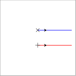
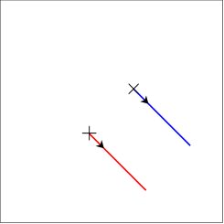
Figure 3: Trajectories of the reduced dynamics law (1.26) with $N=1$ and different initial datum in (1.15), i.e. different $\boldsymbol{Q}_{0}$, for: (i) $\boldsymbol{a}^{0}_{1}=(0.5,0.4)^{T}$ and $\boldsymbol{a}^{0}_{2}=(0.5,0.6)^{T}$ with $\boldsymbol{Q}_{0}=(-0.4\pi,0)^{T}$ (left), (ii) $\boldsymbol{a}^{0}_{1}=(0.4,0.4)^{T}$ and $\boldsymbol{a}^{0}_{2}=(0.6,0.6)^{T}$ with $\boldsymbol{Q}_{0}=(-0.4\pi,0.4\pi)^{T}$ (middle), and (iii) $\boldsymbol{a}^{0}_{1}=(0.6,0.4)^{T}$ and $\boldsymbol{a}^{0}_{2}=(0.4,0.6)^{T}$ with $\boldsymbol{Q}_{0}=(-0.4\pi,-0.4\pi)^{T}$ (right). Here and in the below, we use $+$ and $\times$ in the pictures to denote vortices with winding numbers $+1$ and $-1$, respectively.

Lemma 5.3.

Take $N=2$ in (1.26) and the initial data (1.15) as

$$\boldsymbol{a}^{0}_{1}=(0.5,0.5)^{T}+(\alpha_{0},\beta_{0})^{T},\quad\boldsymbol{a}^{0}_{2}=(0.5,0.5)^{T}-(\alpha_{0},\beta_{0})^{T},$$ (5.10)

$$\boldsymbol{a}_{3}^{0}=(0.5,0.5)^{T}+(\beta_{0},\alpha_{0})^{T},\quad\boldsymbol{a}^{0}_{4}=(0.5,0.5)^{T}-(\beta_{0},\alpha_{0})^{T},$$

with $0<\beta_{0},\alpha_{0}<1$ such that $\boldsymbol{Q}_{0}=\boldsymbol{0}$, then the analytical solution of (1.26) with (1.15) is given as

$$\boldsymbol{a}_{1}(t)=(0.5,0.5)^{T}+(\alpha(t),\beta(t))^{T},\quad\boldsymbol{a}_{2}(t)=(0.5,0.5)^{T}-(\alpha(t),\beta(t))^{T},$$ (5.11)

$$\boldsymbol{a}_{3}(t)=(0.5,0.5)^{T}+(\beta(t),\alpha(t))^{T},\quad\boldsymbol{a}_{4}(t)=(0.5,0.5)^{T}-(\beta(t),\alpha(t))^{T},$$

where ($\alpha(t)$, $\beta(t)$) is the solution of

$$\left\{\begin{aligned} &\dot{\alpha}=2\left(-\partial_{y}F(\alpha-\beta,\beta-\alpha)+\partial_{y}F(2\alpha,2\beta)-\partial_{y}F(\alpha+\beta,\alpha+\beta)\right),\\ &\dot{\beta}=2(\partial_{x}F(\alpha-\beta,\beta-\alpha)-\partial_{x}F(2\alpha,2\beta)+\partial_{x}F(\alpha+\beta,\alpha+\beta)),\end{aligned}\right.$$ (5.12)

with the initial data

$$\alpha(0)=\alpha_{0},\qquad\beta(0)=\beta_{0}.$$ (5.13)

Proof.

By the symmetry of (1.17), we have that $F$ satisfies

$$F(x,y)=F(-x,y)=F(x,-y)=F(y,x).$$ (5.14)

Then, owing to the symmetry of the initial data (5.10) and the symmetry of the equation (1.26), we can take the ansatz that the solution $\boldsymbol{a}=(\boldsymbol{a}_{1},\boldsymbol{a}_{2},\boldsymbol{a}_{3},\boldsymbol{a}_{4})^{T}$ satisfies (5.11). Substituting (5.11) into (1.26) and noting that

$$\boldsymbol{Q}_{0}=2\pi\mathbb{J}(\boldsymbol{a}_{1}^{0}+\boldsymbol{a}_{2}^{0}-\boldsymbol{a}_{3}^{0}-\boldsymbol{a}_{4}^{0})=\boldsymbol{0},$$ (5.15)

we have

$$\dot{\boldsymbol{a}}_{1}=2\mathbb{J}(-\nabla F(\alpha-\beta,\beta-\alpha)+\nabla F(2\alpha,\beta)-\nabla F(\alpha+\beta,\alpha+\beta)).$$ (5.16)

Noting $\dot{\boldsymbol{a}}_{1}=(\dot{\alpha},\dot{\beta})$, we obtain (5.12). ∎

Similar to Lemma 5.3, we can prove the following lemmas:

Lemma 5.4.

Take $N=2$ in (1.26) and the initial data (1.15) as

$$\boldsymbol{a}^{0}_{1}=(0.5,0.5)^{T}+(\alpha_{0},\beta_{0})^{T},\quad\boldsymbol{a}^{0}_{2}=(0.5,0.5)^{T}-(\alpha_{0},\beta_{0})^{T},$$ (5.17)

$$\boldsymbol{a}_{3}^{0}=(0.5,0.5)^{T}+(\alpha_{0},-\beta_{0})^{T},\quad\boldsymbol{a}^{0}_{4}=(0.5,0.5)^{T}-(\alpha_{0},-\beta_{0})^{T},$$

with $0<\beta_{0},\alpha_{0}<1$ such that $\boldsymbol{Q}_{0}=\boldsymbol{0}$, then the analytical solution of (1.26) with (1.15) is given as

$$\boldsymbol{a}_{1}(t)=(0.5,0.5)^{T}+(\alpha(t),\beta(t))^{T},\quad\boldsymbol{a}_{2}(t)=(0.5,0.5)^{T}-(\alpha(t),\beta(t))^{T},$$ (5.18)

$$\boldsymbol{a}_{3}(t)=(0.5,0.5)^{T}+(\alpha(t),-\beta(t))^{T},\quad\boldsymbol{a}_{4}(t)=(0.5,0.5)^{T}-(\alpha(t),-\beta(t))^{T},$$

where ($\alpha(t)$,$\beta(t)$) is the solution of

$$\left\{\begin{aligned} &\dot{\alpha}=2\left(\partial_{y}F(2\alpha,2\beta)-\partial_{y}F(0,2\beta)\right),\\ &\dot{\beta}=2(-\partial_{x}F(2\alpha,2\beta)+\partial_{x}F(2\alpha,0)),\end{aligned}\right.$$ (5.19)

with the initial data (5.13).

Lemma 5.5.

Take $N=2$ in (1.26) and the initial data (1.15) as

$$\boldsymbol{a}^{0}_{1}=(x_{0},0.25)^{T}+(\alpha_{0},\beta_{0})^{T},\quad\boldsymbol{a}^{0}_{2}=(x_{0},0.25)^{T}-(\alpha_{0},\beta_{0})^{T},$$ (5.20)

$$\boldsymbol{a}_{3}^{0}=(x_{0},0.75)^{T}+(\alpha_{0},-\beta_{0})^{T},\quad\boldsymbol{a}^{0}_{4}=(x_{0},0.75)^{T}-(\alpha_{0},-\beta_{0})^{T},$$

with $0<\beta_{0},\alpha_{0}<1$ such that $\boldsymbol{Q}_{0}\neq\boldsymbol{0}$, then the analytical solution of (1.26) with (1.15) is given as

$$\boldsymbol{a}_{1}(t)=(x_{0},0.25)^{T}+(\alpha(t),\beta(t))^{T}-2t\boldsymbol{Q}_{0},\quad\boldsymbol{a}_{2}(t)=(x_{0},0.25)^{T}-(\alpha(t),\beta(t))^{T}-2t\boldsymbol{Q}_{0},$$ (5.21)

$$\boldsymbol{a}_{3}(t)=(x_{0},0.75)^{T}+(\alpha(t),-\beta(t))^{T}-2t\boldsymbol{Q}_{0},\quad\boldsymbol{a}_{4}(t)=(x_{0},0.75)^{T}-(\alpha(t),-\beta(t))^{T}-2t\boldsymbol{Q}_{0},$$

where ($\alpha(t)$,$\beta(t)$) is the solution of

$$\left\{\begin{aligned} &\dot{\alpha}=2\left(\partial_{y}F(2\alpha,2\beta)-\partial_{y}(0,2\beta-0.5)\right),\\ &\dot{\beta}=2(-\partial_{x}F(2\alpha,2\beta)+\partial_{x}F(2\alpha,0.5)),\end{aligned}\right.$$ (5.22)

with the initial data (5.13).

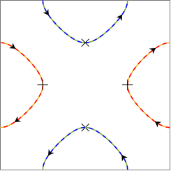
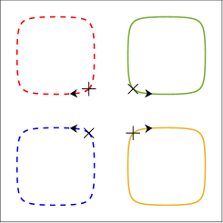
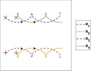
Figure 4: Trajectories of the reduced dynamics law (1.26) with $N=2$ for different initial datum: (i) in (5.10) with $\alpha_{0}=-0.25$ and $\beta_{0}=0$ (left), (ii) in (5.17) with $\alpha_{0}=-0.1$ and $\beta_{0}=0.1$ (middle), and (iii) in (5.20) with $x_{0}=0.15$, $\alpha_{0}=-0.075$ and $\beta_{0}=0$ (right).

To illustrate the solution of (1.26) with the initial data (1.15) for a few special setups, we solve it numerically by adopting the fourth-order Runge-Kutta method with time step $\Delta t=10^{-4}$. Figure 3 plots the solutions of (1.26) with $N=1$ and different initial datum in (1.15), i.e. different $\boldsymbol{Q}_{0}$, to illustrate the dynamics described in Lemma (5.2); and Figure 4 shows the solutions of (1.26) with $N=2$ and different initial datum in (5.10) to illustrate the dynamics described in Lemma 5.3, in (5.17) to illustrate the dynamics described in Lemma 5.4, and in (5.20) to illustrate the dynamics described in Lemma 5.5.

6 Conclusion

A new reduced dynamical law for quantized vortex dynamics of the nonlinear Schödinger equation (NLSE) on the torus with non-vanishing momentum was established when the vortex core size $\varepsilon\to 0$. It is governed by a Hamiltonian flow driven by a renormalized energy on the torus and it collapses to the reduced dynamical law obtained in [10] for NLSE on the torus with vanishing momentum. The key step is to adopt a new canonical harmonic map on the torus to include the effect of the non-vanishing momentum into the dynamics. Extension of the reduced dynamical law for NLSE on torus with arbitrary length and width was discussed. Finally, three first integrals of the reduced dynamical law were presented and analytical solutions were obtained with several initial setups with symmetry.

CRediT authorship contribution statement

Weizhu Bao: Conceptualization, Validation, Supervision, Writing - review & editing. Huaiyu Jian: Conceptualization, Validation, Supervision, Writing - review & editing. Yongxing Zhu: Conceptualization, Methodology, Writing - original draft, Writing - review & editing.

Data availability

No data was used for the research described in the article.

Declaration of competing interest

The authors declare that they have no known competing financial interests or personal relationships that could have appeared to influence the work reported in this paper.

References

- [1] W. Bao, Q. Du, Y. Zhang, Dynamics of rotating Bose-Einstein condensates and its efficient and accurate numerical computation, SIAM J. Appl. Math. 66 (2006) 758–786.
- [2] W. Bao, S. Shi, Z. Xu, Quantized vortex dynamics and interaction patterns in superconductivity based on the reduced dynamical law, Discret. Contin. Dyn. Syst. B 23 (2018) 2265–2297.
- [3] W. Bao, Q. Tang, Numerical study of quantized vortex interactions in the nonlinear Schrödinger equation on bounded domains, Multiscale Model. Simul. 12(2) (2014) 411–439.
- [4] W. Bao, Q. Tang, Numerical study of quantized vortex interaction in the Ginzburg-Landau equation on bounded domains, Commun. Comput. Phys. 14 (2013) 819–850.
- [5] W. Bao, R. Zeng, Y. Zhang, Quantized vortex stability and interaction in the nonlinear wave equation, Physica D 237 (2008) 2391–2410.
- [6] F. Bethuel, H. Brezis, F. Helein, Ginzburg-Landau Vortices, Springer, Cham, 2017.
- [7] F. Bethuel, R. L. Jerrard, D. Smets, On the NLS dynamics for infinite energy vortex configurations on the plane, Rev. Mat. Iberoam. 24(2) (2008) 671–702.
- [8] G. P. Bewley, D. P. Lathrop, K. R. Sreenivasan, Visualization of quantized vortices, Nature 441(2006) 588–588.
- [9] T. Cazenave, Semilinear Schrödinger Equation, Courant Lect. Notes Math., vol. 10, Am. Math. Soc., Providence, Rhode Island, 2003.
- [10] J. E. Colliander, R. L. Jerrard, Ginzburg-Landau vortices: weak stability and Schrödinger equation dynamics, J. Anal. Math. 77(1) (1999) 129–205.
- [11] R. Ignat, R. L. Jerrard, Renormalized energy between vortices in some Ginzburg-Landau models on 2-dimensional Riemannian manifolds, Arch. Ration. Mech. Anal. 239(3) (2021) 1577–1666.
- [12] R. L. Jerrard, Vortex dynamics for the Ginzburg-Landau wave equation, Calc. Var. Partial Differ. Equ. 9(1) (1999) 1–30.
- [13] R. L. Jerrard, H. M. Soner, Dynamics of Ginzburg-Landau vortices, Arch. Ration. Mech. Anal. 142(2) (1998) 99–125.
- [14] R. L. Jerrard, D. Spirn, Refined Jacobian estimates and Gross-Pitaevsky vortex dynamics, Arch. Ration. Mech. Anal. 190(3) (2008) 425–475.
- [15] H. Y. Jian, The dynamical law of Ginzburg-Landau vortices with a pinning effect, Appl. Math. Lett. 13(4) (2000) 91–94.
- [16] H. Y. Jian, B. H. Song, Vortex dynamics of Ginzburg–Landau equations in inhomogeneous superconductors, J. Differ. Equ. 13(1) (2001) 123–141.
- [17] M. Y. Kagan, Modern Trends in Superconductivity and Superfluidity, Springer, Dordrecht, 2013.
- [18] F. H. Lin, Some dynamical properties of Ginzburg-Landau vortices, Commun. Pure Appl. Math. 49(4) (1996) 323–359.
- [19] F. H. Lin, Complex Ginzburg-Landau equations and dynamics of vortices, filaments, and codimension-2 submanifolds, Commun. Pure Appl. Math. 51(4) (1998) 385–441.
- [20] F. H. Lin, Vortex dynamics for the nonlinear wave equation, Commun. Pure Appl. Math. 52(6) (1999) 737–761.
- [21] F. H. Lin, J. X. Xin, On the dynamical law of the Ginzburg-Landau vortices on the plane, Commun. Pure Appl. Math. 52(10) (1999) 1189–1212.
- [22] F. H. Lin, J. X. Xin, On the incompressible fluid limit and the vortex motion law of the nonlinear Schrödinger equation, Commun. Math. Phys. 200(2) (1999) 249–274.
- [23] P. Mironescu, On the stability of radial solutions of the Ginzburg-Landau equation, J. Funct. Anal. 130(2) (1995) 334–344.
- [24] J. C. Neu, Vortex dynamics of the nonlinear wave equation, Physica D 43(2-3) (1990) 407–420.
- [25] J. C. Neu, Vortices in complex scalar fields, Physica D 43(2) (1990) 385–406.
- [26] L. P. Pitaevskii, Vortex lines in an imperfect Bose gas, Sov. Phys. JETP 13(2) (1961) 451–454.
- [27] J. Rubinstein, Self-induced motion of line defects, Q. Appl. Math. 49(1) (1991) 1–9.
- [28] S. Serfaty, Mean field limits of the Gross-Pitaevskii and parabolic Ginzburg-Landau equations, J. Am. Math. Soc. 30(3) (2017) 713–768.
- [29] Y. Zhang, W. Bao, Q. Du, Numerical simulation of vortex dynamics in Ginzburg-Landau-Schrödinger equation, Eur. J. Appl. Math. 18(5) (2007) 607–630.