On the Limits of Cross-Authentication Checks
for GNSS Signals

Abstract

Global navigation satellite systems (GNSSs) are implementing security mechanisms: examples are Galileo open service navigation message authentication (OS-NMA) and GPS chips-message robust authentication (CHIMERA). Each of these mechanisms operates in a single band. However, nowadays, even commercial GNSS receivers typically compute the position, velocity, and time (PVT) solution using multiple constellations and signals from multiple bands at once, significantly improving both accuracy and availability. Hence, cross-authentication checks have been proposed, based on the PVT obtained from the mixture of authenticated and non-authenticated signals.

In this paper, first, we formalize the models for the cross-authentication checks. Next, we describe, for each check, a spoofing attack to generate a fake signal leading the victim to a target PVT without notice. We analytically relate the degrees of the freedom of the attacker in manipulating the victim’s solution to both the employed security checks and the number of open signals that can be tampered with by the attacker. We test the performance of the considered attack strategies on an experimental dataset. Lastly, we show the limits of the PVT-based GNSS cross-authentication checks, where both authenticated and non-authenticated signals are used.

I Introduction

Global navigation satellite systems (GNSSs) provide real-time positioning and timing for various civil and military applications. However, GNSS signals are particularly susceptible to both accidental and intentional interference due to their low received power. Furthermore, civilian GNSS signal and modulation formats are open to the public [1, 2]: therefore, an attacker can compromise location or timing-aware applications by generating fake GNSS signals, leading the receiver into the calculation of a fake location or time [3, 4]. These attacks are referred to as spoofing attacks. Additionally, several works have reported successful attacks even using off-the-shelf hardware [5, 6].

Thus, service providers proposed several authentication mechanisms. On the system side, authentication is strengthened by incorporating into the broadcast GNSS signals specific features, which cannot be predicted and generated by the attacker. An authentication-enabled receiver can then interpret these characteristics to distinguish authentic signals from forgeries. The features can be inserted at two complementary levels: the data level, i.e, on navigation messages, and the ranging level, i.e., on pseudoranges between the satellite and receiver.

Navigation message authentication (NMA) techniques aim at ensuring the authenticity of the content of the navigation messages. Open service NMA (OS-NMA) [7] is a data authentication function for public Galileo E1B signals, in which the message transmitted by the satellites is interleaved with authentication data, generated through a broadcast authentication protocol called timed-efficient stream loss-tolerant authentication (TESLA) [8, 9, 10]. However, NMA-based protocols are vulnerable to secure code estimation and replay (SCER) attacks [11, 12] that estimate the message signature to forge a fake signal in real-time.

Authentication at the ranging level operates on the signal spreading code, de facto authenticating each signal travel time, i.e., the time it takes for the signal to reach the receiver. Spreading code encryption (SCE) techniques are the most reliable options to limit access to GNSS signals, as they make the whole spreading code unpredictable. A SCE solution for Galileo is represented by the commercial authentication service (CAS), which will complement OS-NMA by offering spreading ranging level authentication in the E6 band. The assisted CAS (ACAS), recently presented in [13] and [14], is instead a spreading code authentication (SCA) method based on the navigation data received and authenticated by OS-NMA. For GPS, the chips-message robust authentication (CHIMERA) scheme, [15, 16], aims at jointly authenticating the navigation data and the spreading code of GPS signals for civil usage, implementing both NMA and SCA. This solution replaces a small part of the spreading code with a secret cryptographic sequence, which can be subsequently reproduced by the receivers when they become aware of the key. Navigation message data are instead protected by digitally signing most or all the data. Indeed, ranging level authentication reduces the effectiveness of SCER-type attacks, as discussed in [17]. Thus, in the following, we will refer to signals protected by SCA (or SCE) as authenticated signals, while all the others are open signals.

Both ACAS and CHIMERA present several issues. First, data for range verification is only provided to the receivers a posteriori, therefore they do not allow the verification of the current position, velocity, and time (PVT). To address this, in [18], the authors proposed a strategy where only ACAS is used to derive a continuous, robust, and secure timing service: the application however is limited to static scenarios. A verification method operating on a continuous GPS signal and using a stochastic reachability-based Kalman filter is proposed in [19]. However, this solution relies only on CHIMERA and does not take advantage of signals transmitted by other systems or over different frequency bands.

A second issue is that a receiver using only the authenticated signals to derive the PVT may reduce the solution accuracy and availability. To make the PVT solution more accurate, GNSS receivers typically exploit the signals of all the available frequency bands. Thus, a recent trend considers cross-authentication mechanisms, where, on the receiver side, authenticated signals are combined with open non-authenticated signals, and a consistency check is performed on the obtained solution.

To improve the trustfulness of the PVT, [20] discusses a stepwise approach wherein the receiver exploits the authenticated signals as trust anchors for the complete PVT solution. In particular, the check between signals on the same band but different carrier frequencies has been included in [14] to verify the consistency between Galileo encrypted E6C and E1B open measurements. Still, the effectiveness of the proposed approach degrades when including signals from different systems and in urban scenarios.

In [21], the authors proposed a cross-authentication scheme with the goal of enhancing the Galileo ranging level protection, without relying on CAS, by leveraging on both CHIMERA and OS-NMA single system authentication concepts. Knowing that the GPS and the Galileo reference times are related by the GPS to Galileo time offset (GGTO) [22], they proposed a consistency check between the measured local clock biases and the GGTO retrieved from the navigation messages. However, we will show that it is possible to attack such a mechanism even by tampering with only the open Galileo signals.

In this paper, we investigate the security of cross-authentication for PVT-based checks in GNSS: in particular, we derive spoofing attack strategies targeting cross-authentication schemes showing that such mechanisms do not guarantee the authenticity of the computed solutions. More in detail, the main contributions of the paper are the following.

1. We introduce a new general framework for the PVT cross-authentication checks. In particular, we identify two classes of cross-checks: time-based checks for positioning services and position-based checks for timing. The discussed state-of-the-art mechanisms fit these classes.

2. We introduce the attack strategies that break the cross-authentication checks, and a novel generation time spoofing attack of the signal generation type.

3. We analytically investigate the limits of the new attack, for instance, relating the degrees of the freedom of the attacker in manipulating the victim’s solution to parameters of the transmission/propagation scenario.

4. We analytically evaluate the attack performance considering both a noiseless scenario and a realistic noisy scenario.

5. We test the attacks by using an experimental dataset collected by a Septentrio PolarRx5 receiver.

The rest of this paper is organized as follows. Section II introduces the system model. Section III provides a general model for the PVT-based authentication checks. Then, Section IV describes the proposed attack strategies. Section VI presents the numerical results, obtained from the experimental dataset. Finally, Section VII provides the conclusions.

II System Model

We consider a multi-constellation receiver acquiring signals from $M>1$ constellations. A subset of the received signals is authenticated, i.e., protected by a SCE (or SCA) mechanism. For instance, these may represent a set of Galileo signals protected by CAS in the E6C band or GPS signals protected by CHIMERA in L1 C/A. We assume no fault can happen in the authentication assessment of these signals; thus, the attacker cannot generate new signals to replace the authenticated ones.

In general, the victim receiver obtains signals from $N$ visible satellites: $N_{\mathrm{A}}$ are authenticated while the remaining $N_{\mathrm{O}}=N-N_{\mathrm{A}}$ are open (i.e., non-authenticated). For ease of notation, the authenticated satellites are indexed by $j=1,\ldots,N_{\mathrm{A}}$, while non-authenticated satellites are indexed by $j=N_{\mathrm{A}}+1,\ldots,N$. After the general acquisition and tracking procedures (see, e.g., [23, Ch. 5]), the receiver obtains a vector of pseudoranges measurements $\bm{r}=\left[r_{1},\ldots,r_{\mathrm{N}}\right]^{\mathrm{T}}$.

In nominal conditions, the PVT solution computed by the victim receiver is

$$p=[x,\,y,\,z,\,t_{1},\,\ldots,\,t_{M}]^{\mathrm{T}}\,,$$ (1)

denoting the receiver’s three-dimensional position in Earth-Centered Earth-Fixed (ECEF) coordinates, and the clock biases, one per each time reference. The procedure to obtain (1) is outlined in Appendix A. Indeed, we may consider a single time reference, e.g., one of the GNSS time references or the coordinated universal time (UTC), and relate the others reference, using the respective inter-system bias (ISB) [24, Ch. 21], thus obtaining the PVT solution

$$p=[x,\,y,\,z,\,t]^{\mathrm{T}}\,,$$ (2)

as outlined in Appendix B. However, some of the considered mechanisms use instead the ISB to assess the authenticity of the solution, so, in these cases, we will estimate each clock bias separately from the others, as in (1). On the other hand, when the assessment is based on the receiver position, we will consider the PVT solution to be computed as in (2).

II-A PVT Solution

In this Section, we briefly describe how GNSS receivers typically compute the PVT solution that will be used in the cross-authentication checks.

At each epoch, the PVT solution is computed following an iterative approach, starting from the initial solution $\hat{\bm{p}}~{}=~{}[\hat{x},\hat{y},\hat{z},\hat{t}_{1},\ldots,\hat{t}_{M}]^{\mathrm{T}}$, or $\hat{\bm{p}}~{}=~{}[\hat{x},\hat{y},\hat{z},\hat{t}]^{\mathrm{T}}$, depending on whether we aim to get (1) or (2), respectively. In particular, $\hat{\bm{p}}$ is the PVT computed at the previous epoch or a predefined starting point (cold start). The approach follows a linearization procedure, where the PVT is related to the range by the geometry matrix $\bm{G}$ (see Appendices A and B for details). Thus, given the range measurement of the $j$th signal $r_{j}$ and its estimate $\hat{r}_{j}$, the range residual is

$$\Delta r_{j}=r_{j}-\hat{r}_{j}\,.$$ (3)

Next, observe that the pseudorange displacement $\Delta\bm{r}$ is related to the position displacement $\Delta\bm{p}$ as

$$\Delta\bm{r}=\bm{G}\Delta\bm{p}=\begin{bmatrix}\bm{G}_{\mathrm{A}}\\ \bm{G}_{\mathrm{O}}\end{bmatrix}\Delta\bm{p}\,,$$ (4)

where we decomposed the geometry matrix considering the authenticated and the open signal in $\bm{G}_{\mathrm{A}}$ and $\bm{G}_{\mathrm{O}}$, respectively. From the previous relation, it follows that $\Delta\bm{p}$ can be computed from $\Delta\bm{r}$ as

$$\Delta\bm{p}=(\bm{G}^{\mathrm{T}}\bm{G})^{-1}\bm{G}^{\mathrm{T}}\Delta\bm{r}\triangleq\bm{H}\Delta\bm{r}\,,$$ (5)

where $\bm{H}$ is the Moore-Penrose pseudoinverse of $\bm{G}$, often called also least-squares solution matrix. We remark that the components of matrix $\bm{H}$ depend only on the relative geometry between the user and the $N$ satellites participating in the least-squares computation. Finally the position is updated as $\hat{\bm{p}}^{\prime}=\hat{\bm{p}}+\Delta\bm{p}$, where $\hat{\bm{p}}^{\prime}$ is the starting point for the next iteration.

The iterative procedure continues until either i) the maximum number of iterations is reached or ii) the solution update is smaller than a user-defined step, i.e., $\|\Delta\bm{p}\|<\epsilon$. More details about the procedure and the derivation of each term are reported in the Appendices.

II-B Attacker Model

In this Section, we detail the attacker’s capabilities and operations. We assume that the message data (e.g., atmospheric corrections and ephemeris) are retrieved from a publicly-available authenticated side channel. Additionally, we suppose that the actual victim receiver position is known by the attacker. We take into consideration two types of attacks:

Generation attack:

This attack consists of the generation and transmission of fake GNSS signals, corresponding possibly different PVT solutions than the one computed using the legitimate signals.

Relay attack:

This attack consists of sampling, recording, and relaying the entire modulated signal with unchanged code and data. This attack is sometimes referred to as meaconing.

We remark that the attacker cannot perform a generation attack on authenticated signals, which are protected by SCA (or SCE), because he has no knowledge of the actual spreading code. The only action the attacker can perform on the authenticated signals is a relay attack. On the other hand, the attacker can generate, relay, or selectively delay the open signals, since, in this case, both the spreading code and the message content are entirely public.

We assume that the victim under attack acquires and locks onto the forged signals transmitted by the attacker. This is achieved, for instance, by increasing the transmitting power of the forged signals or canceling the legitimate open ones.

The attacker aims at inducing the victim receiver to obtain as PVT some target position $\bm{p}^{\star}$ instead of the authentic solution $\bm{p}$. To achieve this goal, he tampers the signals propagation times, altering the range residuals $\Delta{\bm{r}}$ by a term $\Delta{\bm{r}_{\mathrm{T}}}$, such that, when under attack, (4) and (5) become respectively

$$\Delta\widetilde{\bm{r}}\triangleq\Delta\bm{r}+\Delta\bm{r}_{\mathrm{T}} =\bm{G}(\Delta\bm{p}+\Delta\bm{p}_{\mathrm{T}})\,,$$ (6)

$$\Delta\widetilde{\bm{p}}\triangleq\Delta\bm{p}+\Delta\bm{p}_{\mathrm{T}} =\bm{H}\Delta\widetilde{\bm{r}}\,.$$ (7)

This means that the range tampering $\Delta\bm{r}_{\mathrm{T}}$ causes a displacement on the PVT solution $\Delta\bm{p}_{\mathrm{T}}$. So, the PVT update due to the attacker spoofing will be

$$\widetilde{\bm{p}}=\hat{\bm{p}}+\Delta\widetilde{\bm{p}}=\hat{\bm{p}}+\Delta\bm{p}+\Delta\bm{p}_{\mathrm{T}}\,.$$ (8)

We remark that the iterative least squares approach to compute the PVT when under attack is approximated by a linear transformation only when the pseudorange displacement $\Delta\bm{r}_{\mathrm{T}}$ introduced by the attacker is small with respect to $\bm{r}$. In Section VI, we will test the effectiveness of the attack by exploiting the linearization procedure and evaluating the performance as a function of the distance between the target and the real position, i.e., the magnitude of the pseudorange displacements to be induced, thus testing the robustness of the linear approximation.

Figure 1: Example of the scenario under attack: $\hat{\bm{p}}$ is the solution at the iteration start, $\bm{p}$ is the legitimate solution, ${\bm{p}}^{\star}$ is the attacker target solution, and $\tilde{\bm{p}}$ is the solution computed by the victim, mixing open and tampered signals.

Fig. 1 shows the displacement of the attacker PVT due to the attacker tampering: in legitimate conditions, starting from $\hat{\bm{p}}$, the receiver would compute $\Delta\bm{p}$ to obtain the legitimate solution $\bm{p}$ (in black). In turn, the attacker wants to lead the receiver to the target $\bm{p}^{\star}$ (in red), thus he tampers the signals, causing the alteration $\Delta\bm{p}_{\mathrm{T}}$. In this case, instead of the true PVT, the victim computes $\tilde{\bm{p}}$, as close as possible to the target $\bm{p}^{\star}$. Notice that Fig. 1 may represent the actual 3D position or the whole PVT vector, i.e., considering points in the $3+M$ space.

For the sake of clarity, we will distinguish between authenticated and non-authenticated ranges residuals, $\Delta\bm{r}_{\mathrm{T,A}}$ and $\Delta\bm{r}_{\mathrm{T,O}}$, that the attacker introduces to the authenticated and non authenticated signals, respectively

$$\Delta\bm{r}_{\mathrm{T}}=\begin{bmatrix}\Delta\bm{r}_{\mathrm{T,A}}\\ \Delta\bm{r}_{\mathrm{T,O}}\end{bmatrix}.$$ (9)

Finally, it is natural to partition the least square matrix as $\bm{H}=[\bm{H}_{\mathrm{A}}\,\bm{H}_{\mathrm{O}}]$, where $\bm{H}_{\mathrm{A}}$ and $\bm{H}_{\mathrm{O}}$ represent the matrix associated to the authenticated and the open signals, respectively. In particular, since the attacker can only perform a relay attack on the authenticated signals, we model the tampering of the attacker on the authenticated ranges as $\Delta\bm{r}_{\mathrm{T,A}}=k\bm{1}$, where $\bm{1}$ is the column vector filled with all ones. Indeed, when performing a generation attack, the attacker sets $k=0$, i.e., only the open signals are actually fake.

III PVT-based Cross-Authentication Checks Models

The receiver computes the PVT solution using both authenticated and non-authenticated ranges. Next, to assess its authenticity, it performs one or more consistency checks on the PVT (or in part of it). We use decision theory to describe the problem and consider the two hypotheses

$$\mathcal{H}_{0}:\;\mbox{PVT is legitimate, signals are legitimate,}$$

$$\mathcal{H}_{1}:\;\mbox{PVT is fake, signals have been tampered with.}$$

The consistency check on the PVT provides one of the two decision

$$\hat{\mathcal{H}}_{0}:\;\mbox{Check passed, PVT is legitimate}$$

$$\hat{\mathcal{H}}_{1}:\;\mbox{Check failed, PVT is not legitimate.}$$

This allows us to define the false alarm and missed detection probabilities as

$$p_{\mathrm{FA}}=P(\hat{\mathcal{H}}_{1}|{\mathcal{H}}_{0})\,$$ (10a)

$$p_{\mathrm{MD}}=P(\hat{\mathcal{H}}_{0}|{\mathcal{H}}_{1})\,.$$ (10b)

In the next Sections, we describe the classes of consistency checks to authenticate the PVT, also related to the required service.

III-A Time-Based Checks for Navigation Services

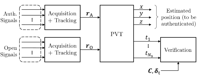
Figure 2: Block scheme of the time-based check.

The receiver collects signals from $M$ different GNSSs, with the PVT solution containing $N_{\rm s}$ clock biases, one per GNSS time reference, thus, $\bm{p}$ is computed as in Appendix A. The time references are related by the ISB, thus the receiver considers the PVT to be authentic if

$$\bm{\theta}_{\mathrm{t}}\triangleq\bm{C}\bm{p}\leq\bm{\delta}_{\mathrm{t}}\,,$$ (11)

where $\bm{C}$ is a matrix that selects and relates a pair of clock biases (with the appropriate sign), while $\bm{\delta}_{\mathrm{t}}$ contains an upper bound of the expected ISB, eventually tuned to meet a predefined false alarm. The mechanism for time-based checks is summarized in Fig. 2. Matrix $\bm{C}$ has $N_{\mathrm{c}}=2\left(M-1\right)$ rows, with $\bm{\delta}_{\mathrm{t}}$ containing $M-1$ upper-bounds on the measured ISB. Therefore, $\bm{C}$ has $M-1$ linearly independent rows. The $i$-th row of $\bm{C}$ is $\bm{c}_{i}$: this will be associated to the $i$-th element of $\bm{\delta}_{\mathrm{t}}$, $\delta_{\mathrm{t},i}$, such that the $i$-th check will be $\theta_{\mathrm{t},i}=\bm{c}_{i}\bm{H}\bm{r}\leq\delta_{\mathrm{t},i}$. For instance, in [21] authors propose to authenticate the computed PVT solution through a time consistency check. In particular, they consider the PVT solution obtained by combining the signals from two constellations, one transmitting authenticated signals and the other transmitting open signals, following the procedure outlined in Appendix A. Then, denoting as $t_{\mathrm{1}}$ and $t_{\mathrm{2}}$ the clock biases associated with the time reference of each constellation, the PVT is authenticated by checking, at the receiver, if the difference $|t_{1}-t_{2}|$ is consistent with the reference ISB, as

$$\left|(t_{\mathrm{2}}-t_{\mathrm{1}})-b-\mathrm{ISB}\right|<T\;,$$ (12)

where $T$ is a threshold that is set by the receiver, and $b$ is a bias set during the calibration phase. More details about the security check and the parameters’ derivation are reported in [21]. The check (12) can be framed in (11), by choosing

$$\bm{C}=\begin{bmatrix}0&0&0&1&-1\\ 0&0&0&-1&1\\ \end{bmatrix}\,,\quad\bm{\delta}_{\mathrm{t}}=\begin{bmatrix}T+b+\mathrm{ISB}\\ T-b-\mathrm{ISB}\end{bmatrix}.$$ (13)

This means that the attacker must craft a $\Delta\bm{r}_{\mathrm{T}}$ that changes the estimated time offset by at most $\bm{\delta_{\mathrm{t}}}$. In the rest of the paper, we will refer to this scheme as ISB-based cross-authentication check.

III-B Position-Based Checks for Timing Services

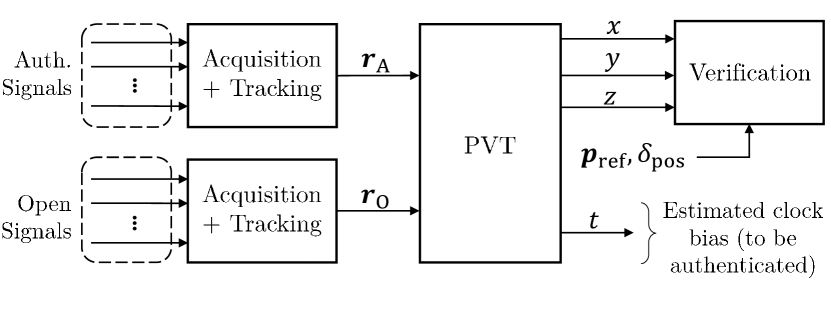
Figure 3: Block scheme of the position-based check.

The goal here is to provide a secure GNSS-based timing source. We assume the receiver knows a priory its position, whose coordinates are denoted by $\bm{p}_{\mathrm{ref}}=[x_{\mathrm{ref}},y_{\mathrm{ref}},z_{\mathrm{ref}}]$: these may be obtained either by computing the PVT using only authenticated ranges, received by a side channel, or it can be simply a priory (e.g., in a static scenario). However, none of these side channels provides a reliable timing correction. Hence, the receiver exploits all the available measurements, both authenticated and open, and obtains the PVT solution $\bm{p}=[x,y,z,t]$, containing the desired clock bias correction, as outlined in Appendix B. To verify its authenticity, the receiver verifies that the reconstructed position is consistent with its a-priori knowledge of the position, verifying that

$${\theta}_{\mathrm{pos}}\triangleq\sqrt{\left(x_{\mathrm{ref}}-x\right)^{2}+\left(y_{\mathrm{ref}}-y\right)^{2}+\left(z_{\mathrm{ref}}-z\right)^{2}}\\ =\sqrt{\bm{\epsilon^{\mathrm{T}}\epsilon}}\leq\delta_{\mathrm{pos}}\,.$$ (14)

where $\bm{\epsilon}\triangleq[x_{\mathrm{ref}}-x,y_{\mathrm{ref}}-y,z_{\mathrm{ref}}-z]$ represents the 3D position displacement with respect to the reference position. The position-based check is summarized in Fig. 3. If the check passes, i.e., the position computed using all the signals is coherent with the reference one, the solution is considered safe and the receiver uses the timing correction from $\bm{p}$ to correct the local clock. An example of such a setting is described in [18].

IV Proposed Attack Strategies

In this Section, we outline the proposed strategies that the attacker uses to alter the PVT solution without alerting the victim receiver. First, we focus on the ideal noiseless scenario, where the received signals of neither the attacker nor the victim are affected by noise. We will generalize the attack for a more realistic scenario in Section V.

To be successful the attacker must i) alter only the non-protected signals, and choose the $\Delta\bm{r}_{\mathrm{T}}$ such that ii) $\Delta\bm{\tilde{p}}$ passes the check employed by the victim, and iii) leads the victim to a PVT solution close to the target $\bm{p}^{\star}$. In this first phase, we assume that the victim receives the signals as intended by the attacker. Moreover, we consider that the attacker knows the pseudorange vector $\bm{r}$ that the victim would measure in the nominal scenario. In Section V, we will analyze the scenario wherein the attacker cannot pre-compensate the channel, and the victim receives a noisier copy of the tampered signal.

In the following Sections, we describe the attacking strategies for the timing and position-based checks.

IV-A Generation Attack Against Time-Based Checks

We consider a legitimate receiver employing the check described in Section III-A, where the PVT solution is considered to be authentic and the clock bias differences are coherent with the ISBs derived from a side channel.

First, we identify the set of feasible solutions that do not raise an alarm at the receiver. Next, we pick the solution that leads the receiver estimated position close to the target position $\bm{p}^{\star}$.

To identify the set of feasible solutions, we have the following result.

Theorem 1.

Given a constraint vector $\bm{\delta}^{\prime}$, the set of feasible solutions for the attacker containing all the range alterations that do not raise an alarm in (11) is the affine space

$$S=\left\{\Delta\bm{r}_{\mathrm{p}}+s\,,s\in\mathcal{N}(\bm{CH}_{\mathrm{O}})\right\}\,,$$ (15)

where $\Delta\bm{r}_{\mathrm{p}}$ is a solution of $\bm{\delta}^{\prime}=\bm{CH}_{\mathrm{O}}\Delta\bm{r}_{\mathrm{T,O}}$, and $\mathcal{N}(\bm{X})$ is the null space of $\bm{X}$. Moreover, it holds

$$\mathrm{dim}({S})=N_{\mathrm{O}}-M+1\;.$$ (16)

Proof.

Now, condition (11) requires

$$\bm{C}\widetilde{\bm{p}}=\bm{C\hat{p}}+\bm{C}\Delta\widetilde{\bm{p}}=\bm{C\hat{p}}+\bm{C}\Delta\bm{p}+\bm{C}\Delta\bm{p}_{\mathrm{T}}\leq\bm{\delta}_{\mathrm{t}}\,.$$ (17)

We assume that, in the nominal scenario, the check (11) is passed, thus, $\bm{C\hat{p}}+\bm{C}\Delta\bm{p}=\bm{\delta}^{\prime\prime}\leq\bm{\delta}_{\mathrm{t}}$: for instance, this models also the case where the defender’s measurements are affected by noise. So, to avoid raising an alarm, the attacker can choose any alteration that induce a change smaller than $\bm{\delta}_{\mathrm{t}}-\bm{\delta}^{\prime\prime}$, i.e., from 17 the shift induced by the attacker is

$$\bm{C}\Delta\bm{p}_{\mathrm{T}}\triangleq\bm{\delta}^{\prime}\,,\;\;\bm{\delta}^{\prime}\leq\bm{\delta}_{\mathrm{t}}-\bm{\delta}^{\prime\prime}\,.$$ (18)

By using (5) and considering that only non-protected signals can be manipulated by the attacker, we have

$$\begin{split}\bm{\delta}^{\prime}=\bm{C}\Delta\bm{p}_{\mathrm{T}}=\bm{C}\bm{H}\Delta\bm{r}_{\mathrm{T}}=\bm{C}\begin{bmatrix}\bm{H}_{\mathrm{A}}&\bm{H}_{\mathrm{O}}\end{bmatrix}\begin{bmatrix}\bm{0}\\ \Delta\bm{r}_{\mathrm{T,O}}\end{bmatrix}\\ =\bm{C}\bm{H}_{\mathrm{O}}\Delta\bm{r}_{\mathrm{T,O}}\;.\end{split}$$ (19)

Being $\bm{\delta}^{\prime}$ under the control of the attacker, he can choose it such that $\bm{\delta}^{\prime}\in\mathcal{R}(\bm{CH}_{\mathrm{O}})$, so that (19) has at least one solution. Indeed, $\mathrm{rank}(\bm{CH}_{\mathrm{O}})=M-1$, since $\bm{C}$ has $M-1$ linearly independent rows. The matrix resulting from the product $\bm{CH}_{\mathrm{O}}$ has size $N_{\mathrm{c}}\times N_{\mathrm{O}}$.

Hence, by the Rouché-Capelli’s theorem, (19) describes a linear undetermined system that admits infinitely many solutions, belonging to the affine space $S$ as defined in (15), where $\Delta\bm{r}_{\mathrm{p}}$ is any particular solution of (19), which can be found, for instance, by Gaussian elimination. Moreover, since the dimension of an affine space is the dimension of its associated linear space, we have

$$\mathrm{dim}(S)=\mathrm{dim}(\mathcal{N}(\bm{CH}_{\mathrm{O}}))\\ =N_{\mathrm{O}}-\mathrm{rank}(\bm{CH}_{\mathrm{O}})=N_{\mathrm{O}}-M+1\,>1\,.$$ (20)

So, each solution of 19 depends on $N_{\mathrm{O}}-M+1$ parameters. ∎

The above Theorem has two main consequences. First, let us consider the worst-case scenario for the attacker, where the legitimate range residuals $\Delta\bm{r}$ already yield $\bm{C}\Delta\bm{p}=\bm{\delta}$. In this case, there is no margin for the attacker that, from 18, has to pick an attack with $\bm{\delta}^{\prime}=0$. Still, (15) shows that it is possible to lead a successful attack, by picking ranges from the null space $\mathcal{N}(\bm{CH}_{\mathrm{O}})$.

Secondly, it shows that the increased number of signals used in the PVT by the legitimate receiver potentially leads to an increased degree of freedom given to the attacker to manipulate the fake PVT solution, since the dimension of the null space increases. However, using more open signals improves the accuracy of the PVT estimation, when under attack. Therefore, a trade-off between accuracy and security is at stake here. Finally, there may be scenarios where $N_{\mathrm{A}}<4$, therefore no fully authenticated PVT solution is available at all. In these cases, the victim receiver has to increase the number of the open signals used for the PVT or not compute any PVT at all.

Next, we derive the actual range alterations that lead the victim receiver to the target position $\bm{p}^{\star}$. We consider the worst-case scenario for the attacker, where $\bm{\delta}^{\prime}=\bm{0}$. In this case, (19) describes a linear homogeneous system whose solutions belong to the linear space $S=\mathcal{N}(\bm{CH_{\mathrm{O}}})$. Indeed, this boils down to the general case by adding in the calculations a range vector related to the particular solution $\Delta\bm{r}_{\mathrm{p}}$. Thus, any solution belonging to $S$ can be written as

$$\Delta\bm{r}_{\mathrm{T}}=\begin{bmatrix}\bm{u}_{1}&\ldots&\bm{u}_{K}\\ \end{bmatrix}\begin{bmatrix}\alpha_{1}\\ \ldots\\ \alpha_{K}\\ \end{bmatrix}=\bm{U}\bm{\alpha}\;,$$ (21)

where $\bm{u}_{1},\ldots,\bm{u}_{K}$ is an orthonormal basis of $S$, $\alpha_{k}\in\mathbb{R}$ $\forall k=1,\ldots,K$, and $K\triangleq\mathrm{dim}\left(S\right)$. Notice that $\bm{U}$ is a matrix with $3+M$ rows and $K$ columns.

Target and fake positions are related by

$$\widetilde{\bm{p}}-\bm{p}^{\star}=\Delta\widetilde{\bm{p}}-\Delta\bm{p}^{\star}=\bm{H}\Delta\bm{r}_{\mathrm{T}}-\left(\Delta\bm{p}^{\star}-\Delta\bm{p}\right)\\ =\bm{H}\bm{U}\bm{\alpha}-\left(\Delta\bm{p}^{\star}-\Delta\bm{p}\right)\;,$$ (22)

where in the last step we used the fact that the attacker will only use the range alterations that do not raise an alarm, i.e., belonging to (15) so having the form in (22).

By imposing the target position to coincide to the fake one, i.e., $\widetilde{\bm{p}}=\bm{p}^{\star}$, we have

$$\bm{H}\bm{U}\bm{\alpha}=\Delta\bm{p}^{\star}-\Delta\bm{p},$$ (23)

and, resorting to the Moore-Penrose pseudoinverse, we obtain

$$\bm{\alpha}^{\star}=\left(\bm{U}^{\mathrm{T}}\bm{H}^{\mathrm{T}}\bm{H}\bm{U}\right)^{-1}\bm{U}^{\mathrm{T}}\bm{H}^{\mathrm{T}}\left(\Delta\bm{p}^{\star}-\Delta\bm{p}\right)\,.$$ (24)

Finally, plugging this in (21), we obtain the target range alteration

$$\Delta\bm{r}_{\mathrm{T}}^{\star}=\alpha^{\star}_{1}\bm{u}_{1}+\ldots+\alpha^{\star}_{K}\bm{u}_{K}\;.$$ (25)

Indeed, as required, this attack will not raise any alarm while taking the victim exactly to $\bm{p}^{\star}$.

Alternatively, by exploiting (22), we can choose the solution directly minimizing the distance between the induced and the target position, among those that do not raise an alarm, i.e.,

$$\Delta\bm{r}_{\mathrm{T}}^{\star}=\operatorname*{arg\,min}_{\Delta\bm{r}_{\mathrm{T}}\in S}\|\bm{H}\Delta\bm{r}_{\mathrm{T}}-\left(\Delta\bm{p}^{\star}-\Delta\bm{p}\right)\|^{2}\,.$$ (26)

Indeed, as long as the space $S$ is not empty, this problem can be solved by numeric methods.

Attack Against the GGTO-based Cross-authentication Check

We consider the authentication procedure in [21] and exploit the previous analysis to derive the attack. The technique proposed in [21] only considers signals from Galileo and GPS, so we have $M=2$. According to (16), we expect to find a space of feasible solutions $S$ with size $\mathrm{dim}\,(S)=N_{\mathrm{O}}-1$. We consider the worst-case scenario for the attacker where $\bm{\delta}^{\prime}=\bm{0}$. Combining (13) and (19) and denoting as $\bm{h}_{\mathrm{O},i}$ the $i$-th row of $\bm{H}_{\mathrm{O}}$, we have

$$\bm{C}\bm{H}_{\mathrm{O}}\Delta\bm{r}_{\mathrm{T,O}}=\bm{0}\Leftrightarrow(\bm{h}_{\mathrm{O},4}-\bm{h}_{\mathrm{O},5})\Delta\bm{r}_{\mathrm{T,O}}=0\,.\\$$ (27)

Thus, $\Delta\bm{r}_{\mathrm{T,O}}$ belongs to the null space $\mathcal{N}(\bm{h}_{\mathrm{O},4}-\bm{h}_{\mathrm{O},5})$. This corresponds to the orthogonal complement to the space generated by column vector $(\bm{h}_{\mathrm{O},4}-\bm{h}_{\mathrm{O},5})^{\mathrm{T}}$, or

$$S=\mathcal{N}(\bm{h}_{\mathrm{O},4}-\bm{h}_{\mathrm{O},5})=\left\langle(\bm{h}_{\mathrm{O},4}-\bm{h}_{\mathrm{O},5})^{\mathrm{T}}\right\rangle^{\perp}\,.$$ (28)

Considering that $\bm{h}_{\mathrm{O},4}$ and $\bm{h}_{\mathrm{O},5}$ are column vectors of length $N_{\mathrm{O}}$, the null space in (28) has clearly size $N_{\mathrm{O}}-1$ and, as expected, $\mbox{dim}(S)=N_{\mathrm{O}}-1$.

IV-B Attack Against Position-Based Checks

We consider the class of checks described in Section III-B. Here, the victim is using GNSS for timing, while it is monitoring its own position, using the procedure outlined in Appendix B, which is used for the security check: for instance, a scenario where GNSS signals are used to synchronize the clock of a local area network (LAN) within one building is presented in [18]. Indeed, in such condition the position is well-known, so the attacker can only tamper the timing estimation, and induce a PVT shift of the type

$$\Delta\bm{p}_{\mathrm{T}}=\begin{bmatrix}\xi_{x}\\ \xi_{y}\\ \xi_{z}\\ c\gamma_{T}\end{bmatrix}=\begin{bmatrix}\xi_{x}\\ \xi_{y}\\ \xi_{z}\\ 0\end{bmatrix}+\begin{bmatrix}0\\ 0\\ 0\\ c\gamma_{T}\end{bmatrix}=\bm{\xi}+\begin{bmatrix}0\\ 0\\ 0\\ c\gamma_{T}\end{bmatrix}\,,$$ (29)

where $c\gamma_{T}$ is the time shift induced by the attacker to the victim clock. To not raise an alarm, by (14) we need $\|\bm{\xi}\|^{2}\leq\delta_{\mathrm{pos}}$.

In the next paragraphs, we will present a relay and a generation attack against the position-based check. Using either one, the attacker is able to induce the target time shift  (29). While a generation attack may be preferable since, for instance, it does not introduce additional noise at the victim due to the attacker receiver noise, we will prove that it can only be performed if $N_{\mathrm{O}}\geq 4$ signals are used by the victim.

Relay Attack Against the Position-Based Check

Starting from 29 the attack can be compute straightly from 4 as

$$\Delta\bm{r}_{\mathrm{T}}=\bm{G}\Delta\bm{p}_{\mathrm{T}}=c\gamma_{T}\bm{1}+G\bm{\xi}\;,$$ (30)

where $\bm{1}$ is a vector of ones with the same size as $\bm{p}$. In the worst-case scenario for the attacker, where $\|\bm{\xi}\|=0$ or, equivalently, $\delta_{\mathrm{pos}}=0$, i.e., no change in the position is tolerated at the legitimate receiver, it yields

$$\Delta\bm{r}_{\mathrm{T}}=c\gamma_{T}\bm{1}\;.$$ (31)

This means that the attacker has to receive, record, and retransmit with some delay both the authenticated and the open signals to induce the required attack, as typically done for the meaconing attack. On the other hand, this also shows that when picking $\bm{\xi}\neq\bm{0}$ we are choosing a solution that differs by (at most) $G\bm{\xi}$ from the meaconing solution.

Finally notice that, as pointed out in Section II-B, this attack can be performed even when the ranges are authenticated by SCE or SCA. Still, this is a viable option only if the attacker is sufficiently close to the victim. Conversely, it may induce a different position calculation, that may alert the victim. However, especially when considering realistic scenarios, relay attacks may introduce additional noise. Thus, if possible, the attacker would rather use a generation attack even for position-based checks. For this reason, in the next paragraph, we will present a generation attack strategy against position-based checks.

Generation Attack Against Position-Based Checks

In this Section, we show how and when it is possible for the attacker to perform a generation-type attack against the position-based check. The attacker aims at introducing a time shift equal to $c\gamma_{\mathrm{T}}$ on the estimated clock bias, as in (31). So, by exploiting the linearization procedure of 5 and combining it with (29), the attacker must choose $\Delta r_{\mathrm{T}}$ to obtain

$$\bm{H}\Delta\bm{r}_{\mathrm{T}}=\begin{bmatrix}0\\ 0\\ 0\\ c\gamma_{T}\end{bmatrix}\,.$$ (32)

Indeed, the range alteration $\Delta\bm{r}_{\mathrm{T}}$ that solves (32) induces a shift only in the time component of the PVT solution computed by the victim. We remark that, for ease of reading, we focus on the worst-case scenario where $\|\xi\|=0$. This can be easily extended also for the case where $\bm{\xi}\neq\bm{0}$, by adding a term $\bm{G}\bm{\xi}$ in (32).

Analogously to the procedure outlined in Section IV-A, we have that the set of feasible solutions of 32 is the affine space

$$S=\left\{\Delta\bm{r}_{\mathrm{p}}+s\,,s\in\mathcal{N}(\bm{H})\right\}\,.$$ (33)

where, from 31, the particular solution is the meaconing attack $\Delta\bm{r}_{\mathrm{p}}=c\gamma_{\mathrm{T}}\bm{1}$.

Indeed, $\bm{H}$ is $4\times N$ and $\mathrm{rank}(\bm{H})=4$, therefore

$$\mathrm{dim}(\mathcal{N}(\bm{H}))=\mathcal{R}(\bm{H})-\mathrm{rank}({\bm{H}})=N-4.$$ (34)

We remark that to compute the PVT, it always holds $N\geq 4$, so $\mathrm{dim}(\mathcal{N}(\bm{H}))\geq 0$. Hence, any range tampering that induces the target time shift, can be written as

$$s=c\gamma_{\mathrm{T}}\bm{1}+\sum_{n=1}^{N-4}\beta_{n}\bm{u}_{n}=c\gamma_{\mathrm{T}}\bm{1}+\bm{U}\bm{\beta}$$ (35)

where vectors $\bm{u}_{1},\ldots,\bm{u}_{N-4}$ form a basis for the null space $\mathcal{N}(\bm{H})$, collected as the columns of the basis matrix $\bm{U}$.

Our aim is to find the range tampering that belongs to $S$ and does not require any alteration on the authenticated ranges. This latter requirement is formalized as

$$\bm{U}_{N_{\mathrm{A}}}\bm{\beta}+c\gamma_{\mathrm{T}}\bm{1}_{N_{\mathrm{A}}}=0\;,$$ (36)

where $\bm{U}_{N_{\mathrm{A}}}$ and $\bm{1}_{N_{\mathrm{A}}}$ collect the first $N_{\mathrm{A}}$ rows of $\bm{U}$ and $\bm{1}$, respectively.

A sufficient condition for (36) to admit at least one solution is that $\bm{U}_{N_{\mathrm{A}}}$, with size $N_{\mathrm{A}}\times N-4$, be left invertible. This happens if $N_{\mathrm{A}}<(N-4)$ or, equivalently, $N_{\mathrm{O}}>4$. Moreover this also assures that $c\gamma_{\mathrm{T}}\bm{1}_{N_{\mathrm{A}}}\in\mathcal{R}(\bm{H})$. Under this condition, the coefficients vector that assures (36) is computed as

$$\bm{\beta}^{\star}=-c\gamma_{\mathrm{T}}\left(\bm{U}_{N_{\mathrm{A}}}^{\mathrm{T}}\bm{U}_{N_{\mathrm{A}}}\right)^{-1}\bm{U}_{N_{\mathrm{A}}}^{\mathrm{T}}\bm{1}_{N_{\mathrm{A}}}\;.$$ (37)

Finally, for the generation attack, the attacker has to pick ranges

$$\Delta\bm{r}^{\star}=c\gamma_{\mathrm{T}}\bm{1}+\sum_{n=1}^{N-4}\beta^{\star}_{n}\bm{u}_{n}\;.$$ (38)

Indeed, by construction of $\bm{\beta}^{\star}$, $\Delta{r}^{\star}_{n}=0$ for $1\leq n\leq N_{\mathrm{A}}$, hence only the open signals need be tampered.

Concluding, we showed that if $N_{\mathrm{O}}\geq 4$, the attacker can exploit the just described procedure to perform a generation-type attack that alters the victim time of a factor $\gamma_{\mathrm{T}}$, generating only the open signals.

V Analysis for the Realistic Scenario

In this Section, we analyze the performance of the attack considering a realistic scenario that takes into account the noise at the victim and the attacker receivers. We remark that, when the attacker performs a generation attack, the fake signals are only affected by the noise added at the victim receiver. On the other hand, when the attacker performs a relay attack, the tampered signals are affected by both the noises produced by the victim’s and the attacker’s receivers. We assume that the channels between the satellites and the receivers, of both the attacker and the victim, are additive white Gaussian noise (AWGN), as well as the channel between the attacker and the victim. We denote with $\sigma_{\mathrm{L}}$ and $\sigma_{\mathrm{A}}$ the noise standard deviations at the victim and attacker receiver, respectively. Moreover, as typically done for GNSS, we assume each channel to be independent, with equal variance.

The noise affects the pseudorange estimations, thus, the covariance matrices of the legitimate and tampered pseudoranges residuals, respectively, are

$$\bm{\Sigma}_{\mathrm{L}}=\mbox{cov}(\Delta\bm{r})\triangleq\sigma^{2}_{\mathrm{L}}\bm{I}_{N}\,,\;\;\;\bm{\Sigma}_{\mathrm{T}}=\mbox{cov}(\Delta\widetilde{\bm{r}})\triangleq\sigma^{2}_{\mathrm{T}}\bm{I}_{N}\,,$$ (39)

where $\sigma^{2}_{\mathrm{T}}=\sigma^{2}_{\mathrm{L}}$ when the attacker performs a generation attack, and $\sigma^{2}_{\mathrm{T}}=\sigma^{2}_{\mathrm{L}}+\sigma^{2}_{\mathrm{A}}$ when he performs a relay attack. Moreover, the legitimate pseudorange residuals are zero-mean, at the convergence of the PVT iterative computation. Taking into account the additional tampering introduced by the attacker, the tampered pseudoranges mean is

$$\mathbb{E}\left[\Delta\bm{\widetilde{r}}|\mathcal{H}_{1}\right]=\mathbb{E}\left[\Delta\bm{r}+\Delta\bm{r}_{\mathrm{T}}\right]=\Delta\bm{r}_{\mathrm{T}}\,.$$ (40)

In the next Sections, we separately consider the attacks to the timing and the position-based checks.

V-A Attacks to the Time-Based Checks

Our aim is to statistically characterize the vector $\bm{\theta}_{\mathrm{t}}$, defined in (11), in realistic conditions. Indeed, $\bm{\theta}_{\mathrm{t}}=\bm{C}\bm{H}\Delta\bm{r}$ is a Gaussian vector since it is derived from the linear combination of the Gaussian vector $\Delta\bm{r}$. Thus, to characterize it, we have to compute its mean and covariance, considering both legitimate and under-attack conditions.

In the legitimate scenario, $\mathcal{H}_{0}$, the mean is

$$\mathbb{E}[\bm{\theta}_{\mathrm{t}}|\mathcal{H}_{0}]=\bm{CH}\mathbb{E}[\Delta\bm{r}|\mathcal{H}_{0}]=0\,,$$ (41)

while the covariance of $\bm{\theta}_{\mathrm{t}}$ in $\mathcal{H}_{0}$ is

$$\begin{split}\bm{\Sigma_{0}}\triangleq\mathbb{E}\left[\bm{\theta}_{\mathrm{t}}\bm{\theta}_{\mathrm{t}}^{\mathrm{T}}|\mathcal{H}_{0}\right]=\mathbb{E}\left[\bm{C}\bm{H}\Delta\bm{r}(\bm{C}\bm{H}\Delta\bm{r})^{\mathrm{T}}|\mathcal{H}_{0}\right]=\\ \bm{C}\bm{H}\mathbb{E}\left[\Delta\bm{r}\Delta\bm{r}^{\mathrm{T}}\right]\bm{H}^{\mathrm{T}}\bm{C}^{\mathrm{T}}=\sigma_{\mathrm{L}}^{2}\bm{C}\bm{H}\bm{H}^{\mathrm{T}}\bm{C}^{\mathrm{T}}\,,\end{split}$$ (42)

where, in the last step, we used the definition of $\bm{\Sigma}_{L}$ given in (39).

For the under-attack scenario, $\mathcal{H}_{1}$, the mean is given by

$$\mathbb{E}[\bm{\theta}_{\mathrm{t}}|\mathcal{H}_{1}]=\bm{C}\bm{H}\Delta\bm{r}_{\mathrm{T}}\triangleq\bm{\mu}\,,$$ (43)

while, analogously to (42), the covariance of $\bm{\theta}_{\mathrm{t}}$ in $\mathcal{H}_{1}$ is

$$\begin{split}\bm{\Sigma_{1}}\triangleq\mathbb{E}\left[\bm{\theta}_{\mathrm{t}}\bm{\theta}_{\mathrm{t}}^{\mathrm{T}}|\mathcal{H}_{1}\right]=\sigma_{\mathrm{T}}^{2}\bm{C}\bm{H}\bm{H}^{\mathrm{T}}\bm{C}^{\mathrm{T}}\,.\end{split}$$ (44)

where the last equality follows from the definition of $\bm{\Sigma}_{T}$ given in (39). Moreover, the attack to the time-based check described in Section IV-A is a generation attack, thus $\sigma^{2}_{\mathrm{T}}=\sigma^{2}_{\mathrm{L}}$.

The false alarm and miss detection probabilities are, respectively,

$$p_{\mathrm{FA}} =\mathrm{P}\left[\bigcup_{i=1}^{N_{\mathrm{c}}}\{\theta_{\mathrm{t},i}>\delta_{\mathrm{t},i}\}|\mathcal{H}_{0}\right]=1-\mathrm{P}\left[\bigcap_{i=1}^{N_{\mathrm{c}}}\{\theta_{\mathrm{t},i}\leq\delta_{\mathrm{t},i}\}|\mathcal{H}_{0}\right],$$ (45)

$$p_{\mathrm{MD}} =\mathrm{P}\left[\bigcap_{i=1}^{N_{\mathrm{c}}}\{\theta_{\mathrm{t},i}\leq\delta_{\mathrm{t},i}\}|\mathcal{H}_{1}\right].$$ (46)

We remark that, in general, metrics $\theta_{\mathrm{t},i}$ and $\theta_{\mathrm{t},j}$, with $i\neq j$, are not statistically independent.

Attack Against the ISB-based Cross-authentication Check

We consider now the check of [21], where only Galileo and GPS are considered. First, we neglect the bias $b+GGTO$, which can be subtracted in advance from one measurement. So, it yields $\delta_{\mathrm{t},1}=\delta_{\mathrm{t},2}=T$. Moreover, from 13, $\bm{c}_{1}=-\bm{c}_{2}$, thus also $\theta_{\mathrm{t},1}=-\theta_{\mathrm{t},2}$, and (45) becomes

$$\begin{split}p_{\mathrm{FA}}&=1-P(\theta_{\mathrm{t},1}<T\wedge\theta_{\mathrm{t},2}<T|\mathcal{H}_{0})\\ &=1-P(-\delta_{1}<\theta_{\mathrm{t},1}<T|\mathcal{H}_{0})=2Q(T/\sigma_{0})\;,\end{split}$$ (47)

where $\sigma_{0}=\sigma_{\mathrm{L}}\sqrt{\bm{c}_{1}\bm{H}\bm{H}^{\mathrm{T}}\bm{c}_{1}^{\mathrm{T}}}$. Next, we can invert the above relation to computing the threshold values as a function of the $p_{\mathrm{FA}}$ set by the receiver,

$$T=\sigma_{0}\mathrm{Q}^{-1}\left(\frac{1}{2}p_{\mathrm{FA}}\right)\,.$$ (48)

Analogously, calling $\mu_{1}$ and $\mu_{2}$ the first and second element of $\bm{\mu}$, respectively, the miss detection probability is

$$\begin{split}p_{\mathrm{MD}}&=P(\theta_{\mathrm{t},1}\leq\delta_{\mathrm{t},1}\wedge\theta_{\mathrm{t},2}\leq\delta_{\mathrm{t},2}|\mathcal{H}_{1})\\ &=\mathrm{Q}\left(\frac{-T-\mu_{1}}{\sigma_{1}}\right)-\mathrm{Q}\left(\frac{T-\mu_{1}}{\sigma_{1}}\right)\\ &=\mathrm{Q}\left(-\frac{\sigma_{0}}{\sigma_{1}}\mathrm{Q}^{-1}\left(\frac{1}{2}p_{\mathrm{FA}}\right)-\frac{\mu_{1}}{\sigma_{1}}\right)-\\ -&\mathrm{Q}\left(\frac{\sigma_{0}}{\sigma_{1}}\mathrm{Q}^{-1}\left(\frac{1}{2}p_{\mathrm{FA}}\right)-\frac{\mu_{1}}{\sigma_{1}}\right)\;,\end{split}$$ (49)

where $\mu_{1}=-\mu_{2}=\bm{c}_{1}\bm{H}\Delta\bm{r}_{\mathrm{T}}$ and $\sigma_{1}=\sigma_{\mathrm{T}}\sqrt{\bm{c}_{1}\bm{H}\bm{H}^{\mathrm{T}}\bm{c}_{1}^{\mathrm{T}}}$. Thus, (49) shows the missed detection probability as a function of the false alarm, legitimate and attacker channel noises, and $\bm{\mu}$. In particular, $\bm{\mu}$ is also related to the range alteration induced by the attacker, which is a function of the distance between the true solution $\bm{p}$ and the target $\bm{p}^{\star}$.

In a generation attack scenario, where $\sigma_{0}=\sigma_{1}$, for small values of $\mu_{1}$, from 49 we get $p_{\mathrm{MD}}=p_{\mathrm{FA}}$, which means that fake signals are indistinguishable from the legitimate ones. This shows that the success probability depends on $\mu_{1}$, the amount of displacement induced by the attacker, so that the more the attacker tries to tamper with the signals, the easier it is for the victim to detect the attack. For instance, if we consider a relay attack for position spoofing, as selective delay, then $\sigma_{1}\gg\sigma_{0}$, i.e., the noise standard deviation of the tampered pseudoranges is higher than that of the legitimate ones, $p_{\mathrm{MD}}\rightarrow 0$ for any chosen $p_{\mathrm{FA}}$, thus the receiver is always able to detect the attack. In Section VI-C we will provide a numerical evaluation of these observations.

V-B Attacks to the Position-Based Checks

Our aim is to statistically characterize the term ${\theta}_{\mathrm{pos}}$ in (14), in a realistic environment, i.e., when the measurements are affected by noise. In particular, we aim at relating security performance, i.e., false and miss detection, to the channel noise in the legitimate and under-attack scenarios, $\sigma_{\mathrm{L}}^{2}$ and $\sigma_{\mathrm{T}}^{2}$. Notice that, in the legitimate case, this problem is equivalent to the general problem of characterizing the position accuracy for GNSS.

From (14), we can write

$$\theta_{\mathrm{pos}}^{2}=\bm{\epsilon}^{\mathrm{T}}\bm{\epsilon}\;,$$ (50)

where $\bm{\epsilon}$ is the 3D position displacement with respect to the reference position. We remark that the reference position with coordinates ($x_{\mathrm{ref}},y_{\mathrm{ref}},z_{\mathrm{ref}}$) is assumed to be known without error. Thus, to characterize the performance of the test (14) we model term $\bm{\epsilon}$ first. Indeed, $\bm{\epsilon}$ is a Gaussian vector since the position is derived as a linear combination of the Gaussian random vector $\Delta\bm{r}$, as in (5). In the legitimate case, we have

$$\mathbb{E}[\bm{\epsilon}|\mathcal{H}_{0}]=0\;,$$ (51)

since the PVT solution is expected to converge to the reference position itself. For the covariance we have

$$\mathbb{E}[\bm{\epsilon}\bm{\epsilon}^{\mathrm{T}}|\mathcal{H}_{0}]=\sigma^{2}_{\mathrm{L}}\bm{H}_{1-3}\bm{H}_{1-3}^{\mathrm{T}}\;,$$ (52)

where the subscript of $\bm{H}_{1-3}$ refers to the fact that we are considering only rows 1, 2, and 3 of $\bm{H}$.

Under attack, we have

$$\mathbb{E}[\bm{\epsilon}|\mathcal{H}_{1}]=\bm{H}_{1-3}\Delta\bm{r}_{\mathrm{T}}\;,$$ (53)

and, for the covariance,

$$\mathbb{E}[\bm{\epsilon}\bm{\epsilon}^{\mathrm{T}}|\mathcal{H}_{0}]=\sigma^{2}_{\mathrm{T}}\bm{H}_{1-3}\bm{H}_{1-3}^{\mathrm{T}}\;.$$ (54)

Note that (50) is a quadratic form, so we can take advantage of the following Theorem.

Theorem 2.

The random variable $\theta_{\mathrm{pos}}^{2}=\bm{\epsilon}^{\mathrm{T}}\bm{\epsilon}$, with $\bm{\epsilon}\sim\mathcal{N}\left(\bm{\mu},\bm{\Sigma}\right)$, can be written as

$$\theta_{\mathrm{pos}}^{2}=\left(\bm{u}+\bm{b}\right)\bm{\Lambda}\left(\bm{u}+\bm{b}\right)=\sum_{i}^{3}\lambda_{i}(u_{i}+b_{i})^{2}\;,$$ (55)

where $\bm{u}\sim\mathcal{N}\left(\bm{0},\bm{I}_{3}\right)$, $\bm{\Lambda}$ is the diagonal matrix obtained from the decomposition $\bm{\Sigma}=\bm{P}\bm{\Lambda}\bm{P}^{\mathrm{T}}$ and $\bm{b}^{\mathrm{T}}=\bm{P}^{\mathrm{T}}\bm{\Sigma}^{-\frac{1}{2}}\bm{\mu}$. Hence, $\theta_{\mathrm{pos}}^{2}$ can be expressed as the linear combination of non-central chi-square random variables of degree 1, with non-centrality parameter $b_{i}^{2}$.

Proof.

The proof can be found in [25, Ch. 3], for the quadratic form $Q(\bm{X})=\bm{X}^{\mathrm{T}}\bm{A}\bm{X}$, but using $\bm{A}=\bm{I}$. ∎

Indeed, in the legitimate case, $\epsilon$ has zero mean, thus, $\theta^{2}$ is actually the linear combination of (central) chi-square random variables of degree $1$. Still, it is not possible to derive the closed-form expression for either the false alarm or miss detection probabilities, thus relating the metric value, $\theta_{\mathrm{pos}}$ to the chosen threshold.

For an application-oriented (but approximate) derivation of such relation we could exploit the definition of geometric dilution of precision (GDOP) [23, Ch. 7]. First, we rotate the reference system to have the first three coordinates pointing to the east, north, up (ENU) reference frame. Next, repeating the steps in (52), we get as position error

$$\mathbb{E}\left[\Delta\bm{p}\Delta\bm{p}^{\mathrm{T}}\right]=\sigma^{2}_{L}\bm{H}\bm{H}^{\mathrm{T}}=\sigma^{2}_{L}\left(\bm{G}^{\mathrm{T}}\bm{G}\right)^{-1}.$$ (56)

Hence, taking the trace operation, we define the GDOP as

$$\mathrm{GDOP}\triangleq\frac{1}{\sigma_{L}}\sqrt{\sigma_{\mathrm{E}}^{2}+\sigma_{\mathrm{N}}^{2}+\sigma_{\mathrm{U}}^{2}+\sigma_{\mathrm{t}}^{2}}\;,$$ (57)

where $\sigma_{\mathrm{E}}^{2}$, $\sigma_{\mathrm{N}}^{2}$, and $\sigma_{\mathrm{U}}^{2}$ are the variances associated respectively with the error along the East, North, and vertical directions while $\sigma_{\mathrm{t}}^{2}$ is the error for the clock bias (measured in meters). To focus on the position error, it is useful to consider the position dilution of precision (PDOP)

$$\mathrm{PDOP}\triangleq\frac{1}{\sigma_{L}}\sqrt{\sigma_{\mathrm{E}}^{2}+\sigma_{\mathrm{N}}^{2}+\sigma_{\mathrm{U}}^{2}}\;,$$ (58)

These terms are used to model, and therefore also to predict, the positioning error since the dilution of precision (DOP) values are related to the pseudorange noise and the geometry. Thus, low DOP values are typically associated with high PVT accuracy. An additional in-depth discussion of the DOP and their derivation can be found in [24, Ch. 21].

Hence, it is possible to use this characterization to describe $p(\theta_{\mathrm{pos}}|\mathcal{H}_{0})$ and $p(\theta_{\mathrm{pos}}|\mathcal{H}_{1})$. Still, these estimates would be based only on an approximate model which is not suited for security analysis. The performance of the position check will be therefore evaluated only numerically, in Section VI-C.

VI Numerical Results

In this Section, we assess the performance of the proposed attack against the authentication mechanism discussed in Section III. More in detail, first we describe the data collection procedure and the validation phase. Next, we test both the attacks of Section IV, considering both noiseless and noisy scenarios.

VI-A Data Collection

The dataset was built by collecting signals from a quasi-urban environment with a Septentrio PolarRx5 receiver connected to an A42 Hemisphere antenna. In particular, the measurements were collected from our lab window sill ($45.408^{\circ}\,$N, $11.894^{\circ}\,$E, altitude $30\text{\,}\mathrm{m}$ above the sea level).

The receiver output was post-processed obtaining a dataset of measurements from different constellations. We focused on GPS L1 C/A and Galileo E1 BC. The dataset, contained $10\text{\,}\mathrm{min}$ of measurements, collected with a frequency of $1\text{\,}\mathrm{Hz}$, for a total of 600 PVT epochs. We consider the GPS signals as authenticated (e.g., by CHIMERA) and the Galileo signals as open, and we collected signals from $N=8$ different satellites in view, with $N_{\mathrm{A}}=3$ and $N_{\mathrm{O}}=5$.

More in detail, for each considered epoch, the dataset contained: the pseudoranges measurements, the satellite clock biases, the tropospheric and the ionospheric delays (estimated using the Klobuchar model [26]), and the satellite positions. Satellite clock biases, atmospheric delays, and satellite positions were derived from the respective navigation message.

To test the performance of the attacks, we implemented a PVT computation block operating as summarized in the Appendices, following the description of [27, Ch. 8].

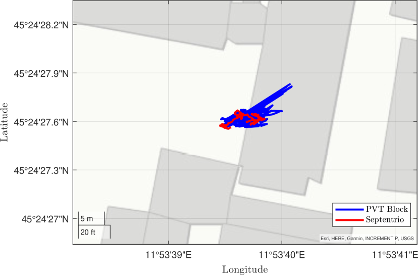
Figure 4: Validation of our PVT block: position computed using our PVT block (blue) and the Septentrio’s software (red).

To validate our PVT block, we report in Fig. 4 respectively the positions computed by the Septentrio receiver, in blue, and those computed by our PVT block, in red. The positions obtained from the Septentrio receiver are slightly more precise than ours: the error standard deviations were $3.03\text{\,}\mathrm{m}$ and $3.13\text{\,}\mathrm{m}$ using, respectively, the Septentrio receiver and our PVT block.

VI-B Attacks in Ideal Scenario Conditions

We now present the attack performance in the noiseless scenario, thus $\sigma_{\mathrm{L}}=\sigma_{\mathrm{T}}=0$, distinguishing between the attack to the time-based and the position-based checks.

Attack Against the Time-Based Check

We present the results of the proposed attack. In particular, we use the following procedure, where at each epoch we

1. compute the PVT solution by using the legitimate measurements (legitimate case);

2. chose the target position $\bm{p}^{\star}_{1}$;

3. solve problem (26), obtaining the tampered ranges $\Delta\bm{\widetilde{r}}$;

4. feed the tampered ranges to the PVT block;

5. check the authenticity of the solution using the ISB-based cross-authentication check (12).

In particular, we set the target position $\bm{p}^{\star}_{1}$ at $45.398\text{\,}\mathrm{\SIUnitSymbolDegree}$ N, $11.876\text{\,}\mathrm{\SIUnitSymbolDegree}$ E, with altitude $12\text{\,}\mathrm{m}$ (Prato della Valle square, Padua, Italy). The distance between the legitimate and the target position is roughly $1.7\text{\,}\mathrm{km}$.

Notice that, between steps 3) and 4) we omitted the actual fake signal generation and the processing of the victim on the received signal. This means that we assumed that, under attack, the victim processes the tampered signal as intended by the attacker. Still as experimentally proved, e.g., in [5] and [6], it is indeed feasible to induce to the victim the fake signals, hence we skipped these steps.

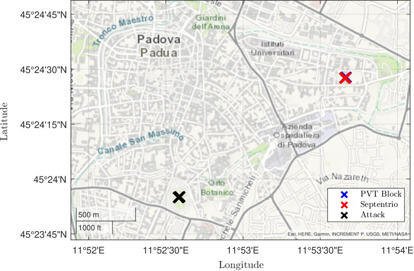
Figure 5: Positions computed in the legitimate (blue) and under attack scenario (black), compared to the ground truth (red). The position computed in the under-attack scenario coincides with the target $\bm{p}^{\star}$.

Fig. 5 shows the positions computed in the legitimate and under-attack scenarios: the attacker is always able to induce the target position and only negligible errors are observed with respect to the target position. No issue has been observed in terms of availability, i.e., all the fake ranges led to the computation of a PVT.

Figure 6: Metric for the check (12): the metric computed under attack (black) is superimposed to the one computed in the legitimate case (red).

Fig. 6 shows the difference between the clock biases $t_{\mathrm{O}}$ and $t_{\mathrm{A}}$ used in the security check (12), computed respectively in the legitimate and under-attack case. Indeed, the check cannot distinguish the legitimate from the under-attack scenario, since the actual differences between legitimate and fake are well below the standard deviation of the metric itself. Hence, for any threshold $T$, the check cannot effectively detect the attack. For these reasons, we conclude that our attack can spoof the victim’s position without being detected.

Fig. 7 shows instead the detection error trade-off (DET) curves for different distances between target and actual position. Indeed as this distance increases, it becomes easier for the victim to detect the spoofing attack. In particular, the attack success probability rapidly decreases for distances higher than $10\text{\,}\mathrm{km}$. This is in line with our observations in Section II-B, confirming that the linearization procedure is not reliable to design the attack if the target position is too far from the real one. Still, we remark that it may not be reasonable for the attacker to consider the target position too far since other signals of opportunity may be exploited by the victim to check the computed position.

Figure 7: DET curves for different distances between legit and target positions, for the time-based cross-authentication against the proposed generation attack.

Attack Against the Position-Based Check

We report the results of the attacks against the position cross-authentication checks, discussed in Section IV-B for the noiseless scenario. In particular, three different attacks are considered (Table I), with different induced time shifts and attack start times.

TABLE I: Parameters of the attack to the position cross authentication check: attack starts $t_{\mathrm{start}}$ and additional clock biases $\Delta t-\Delta t_{\mathrm{L}}$.

	Attack 1	Attack 2	Attack 3
$t_{\mathrm{start}}$	$60\text{\,}\mathrm{s}$	$100\text{\,}\mathrm{s}$	$150\text{\,}\mathrm{s}$
$\Delta t-\Delta t_{\mathrm{L}}$	$30\text{\,}\mu\mathrm{s}$	$10\text{\,}\mu\mathrm{s}$	$5\text{\,}\mu\mathrm{s}$

Fig. 8 shows the results of the step-change on the clock bias estimated by the victim. This represents a best-case scenario for the defender, since, typically, the time shift is induced in a ramp-like manner (e.g., see the classification of [28]). Indeed, if the considered attacks are successful, also the more sophisticated attacks will be successful as well. During the tests, all the considered attacks achieve their aim, inducing the target time shifts. On the other hand, consider the actual position check, no significant position deviation is induced by any of the attacks, since the deviation is at the cm-level, well below the actual accuracy of the receiver. Again, none of these attacks would be detected by the victim using the considered cross-authentication checks.

Figure 8: Effect of the time attack on the clock bias estimated by the victim: $\Delta t$ for the legitimate case (red), for Attack 1 (green), 2 (blue), and 3 (purple), whose parameters are reported in Table I.

VI-C Results with Noisy Measurements

In this Section, we evaluate the performance of the proposed attack in noisy conditions, distinguishing between time-based and position-based checks.

Starting from the experimental dataset, we run a Montecarlo simulation, repeating each experiment 35 times, therefore obtaining in total 21 000 PVT measurements.

Attacks Against the Time-Based Check

As proved in Section IV-A, we show that it is possible for the attacker to lead a successful attack using a generation attack.

We repeat the same attack simulation procedure adopted for the noiseless scenario but, between steps 3) and 4), we add AWGN to both the legitimate and the fake pseudoranges, according to the noise standard deviation at the victim receiver $\sigma_{\mathrm{L}}$, with $\sigma_{\mathrm{L}}=0,1,2,4,$ and $9\text{\,}\mathrm{m}$. We remark that, in this case, the attacker performs a generation attack, thus pseudoranges are only affected by the noise at the victim receiver. In general, a reasonable value for the noise standard deviation is $7.1\text{\,}\mathrm{m}$ [23, Ch. 7]. To evaluate the attack performance, we consider a target position $25.5\text{\,}\mathrm{km}$ away from the victim receiver location.

Fig. 9 reports the DET curve for the generation attack against time-based checks, showing the miss detection probability $p_{\mathrm{MD}}$ as a function of the false alarm probability $p_{\mathrm{FA}}$ and various values of $\sigma_{\mathrm{L}}$. We notice that, as the noise at the victim receiver increases, the victim becomes unable to distinguish between legitimate and fake signals. Still, the results confirm that the check is not fully reliable even when the noise is minimum since, even in this condition, to get $p_{\mathrm{MD}}<10^{-2}$ it would yield $p_{\mathrm{FA}}\approx 0.88$, thus rejecting most of the legitimate signals.

Figure 9: DET curves with for the generation attack against time-based checks, when the attack target position is $25.5\text{\,}\mathrm{km}$ away from the victim location, for different values of $\sigma_{\mathrm{L}}$.

Attacks Against the Position-Based Check

As discussed in Sections IV-B and IV-B, if $N_{\mathrm{O}}<4$ only a relay attack can induce the desired clock-shift while keeping low the probability of being detected. Conversely, when $N_{\mathrm{O}}\geq 4$, also a generation attack can be used to achieve the same goal. It is worth noting that, when both the relay and the generation attack are viable, the latter is always the preferred option, since it involves signal generation instead of retransmission, and, as a result, the attacker does not introduce additional noise to achieve a better performance in terms of $p_{\mathrm{FA}}$ and $p_{\mathrm{MD}}$, as will be discussed in this Section.

First, we consider the relay-type attack described in Section IV-B. Indeed, this represents the worst case for the attacker. To show the attack performance, we add noise only to the tampered ranges, so we consider $\sigma_{\mathrm{L}}=0$. Thus, the fake pseudoranges variance is $\sigma^{2}_{\mathrm{T}}=\sigma^{2}_{\mathrm{A}}$.

We consider the scenarios where the attacker aims to induce a shift in the estimated clock bias $\Delta t-\Delta t_{\mathrm{L}}=$10\text{\,}\mathrm{\SIUnitSymbolMicro s}$$. No relevant difference was observed when considering $\Delta t-\Delta t_{\mathrm{L}}=5$ and $30\text{\,}\mathrm{\SIUnitSymbolMicro s}$. In all the considered scenarios, when receiving the tampered signal, the victim computes the clock bias set by the attacker, with only negligible error. Hence whenever no alarm was raised, the attacks were successful.

Fig. 10 reports the DET curves of the attack for several values of $\sigma_{\mathrm{A}}$. Indeed, for $\sigma_{\mathrm{A}}=0$, thus simulating an attacker able to perform a relay attack without adding any additional noise, tampered and legitimate signals are indistinguishable. On the other hand, as $\sigma_{\mathrm{A}}$ increases, it is easier for the victim to detect the attack. Still, even when $\sigma_{\mathrm{A}}=$9\text{\,}\mathrm{m}$$, the check is only partially effective since to get low values of missed detection the victim experience high false alarm: for instance to get $p_{\mathrm{MD}}<10^{-3}$ (not such a low value for a security application) the victim would obtain a $p_{\rm FA}>0.2$.

Figure 10: DET curves for the relay attack against the position cross-authentication check, for $\Delta t-\Delta t_{\mathrm{L}}=$10\text{\,}\mathrm{\SIUnitSymbolMicro s}$$, for several values $\sigma_{\mathrm{A}}$ and $\sigma_{\mathrm{L}}$ fixed.

Concerning the generation attack against the time-based check, we carried out attack simulations adding the AWGN of the victim receiver to both fake and legitimate ranges, with $\sigma_{\mathrm{L}}=0,1,2,4,$ and $9\text{\,}\mathrm{m}$. For all the considered values of noise standard deviation, the fake ranges resulted to be indistinguishable from the legitimate ones, and all the DET curves collapsed to the line $p_{\rm FA}=p_{\rm MD}$.

VII Conclusion

In this work, general attack strategies targeting cross-authentication PVT-based mechanisms were presented. In such mechanisms, the victim receiver computes the PVT using all the available signals, both open and authenticated and tries to assess the authenticity of the computed PVT using some a priori information. In particular, we focused on two classes of checks: the timing cross-authentication, such as [21], where the check is performed verifying if the clock biases relative to each system are related to the actual ISBs; the position cross-authentication, that may be used for a timing service, where the PVT is considered to be authentic if it leads (sufficiently close) to the expected position. For both scenarios, we show that the attacker leads the victim to a chosen target PVT solution, i.e., to a target 3D position or clock correction. We show that the success of the attack depends on both the number of open signals used by the receiver and the attacker conditions. Still, under realistic conditions, the attack is shown to be successful.

We considered both noiseless and noisy scenarios: in the latter, the receiver obtains a noisier replica of the signal tampered with by the receiver. Numerical results confirm the effectiveness of the attack in both the considered scenarios, showing that such a class of security checks is not able to protect the receiver effectively.

In several practical scenarios, less than 4 authenticated signals may be received so that the receiver cannot compute a PVT based on the authenticated signals solely. Our work shows that it is not possible to extend the authentication to open signals by using PVT-based consistency checks, so the receiver can either choose to compute a non-secure PVT or to not perform navigation at all.

Appendix A PVT Computation with Separate Time References

We describe the PVT linearization procedure and the derivation of each term needed to update the PVT during the iterative approach, to compute the terms of 5.

From the received signal, we derive the pseudorange vector ${\bm{r}}$. For ease of reading, we consider only signals from two systems: hence the PVT will contain entries $t_{\mathrm{1}}$ and $t_{\mathrm{2}}$, the clock biases associated with each of the time references, e.g., to the GPS system time (GPST) and Galileo system time (GST). In particular, the receiver collects $N_{1}$ signals from the first constellation and $N_{2}=N-N_{1}$ from the latter.

In general, each pseudorange is modeled by

$$r_{j}=\rho_{j}+ct_{j}-ct_{\mathrm{1}}\mathbbm{1}_{\mathrm{1}}(j)-ct_{\mathrm{2}}\mathbbm{1}_{\mathrm{2}}(j)+D_{\mathrm{atm},j}+\eta\,,$$ (59)

where $\rho_{j}$ is the geometric range, i.e., the Euclidean distance between the (estimated) receiver position and the $j$th satellite position, with coordinates $(x_{j},y_{j},z_{j})$, defined as

$$\rho_{j}\triangleq\sqrt{(x_{j}-x)^{2}+(y_{j}-y)^{2}+(z_{j}-z)^{2}}\,,$$ (60)

$c$ is the speed of light, $t_{j}$ is the satellite clock bias, $D_{\mathrm{atm},j}$ models the atmospheric delays, and $\eta$ models the remaining errors, considered as noise. The indicator functions $\mathbbm{1}_{\mathrm{1}}(j)$ and $\mathbbm{1}_{\mathrm{2}}(j)$ are introduced to identify the satellite constellations, i.e., $\mathbbm{1}_{\mathrm{1}}(j)=1$ if satellite $j$ belongs to the first constellation and 0 otherwise, while $\mathbbm{1}_{\mathrm{2}}(j)=1$ if satellite $j$ belongs to the second and is 0 otherwise. Notice that (approximations of) the satellites’ positions, $x_{j}$, $y_{j}$, and $z_{j}$, $t_{j}$, and $D_{\mathrm{atm},j}$, are retrieved directly from the navigation messages.

Next, we introduce the terms

$$a_{x,j}\triangleq\frac{x_{j}-\hat{x}}{\hat{\rho}_{j}},\hskip 11.38092pta_{y,j}\triangleq\frac{y_{j}-\hat{y}}{\hat{\rho}_{j}},\hskip 11.38092pta_{z,j}\triangleq\frac{z_{j}-\hat{z}}{\hat{\rho}_{j}}\,,$$ (61)

which represent the components of the unit vector pointing from the (approximate) receiver to the $j$th satellite position. This allows us to introduce the geometry matrix

$$\bm{G}\triangleq\begin{bmatrix}a_{x,1}&a_{y,1}&a_{z,1}&1&0\\ \vdots&\vdots&\vdots&\vdots&\vdots\\ a_{x,N_{1}}&a_{y,N_{1}}&a_{z,N_{1}}&1&0\\ a_{x,N_{1}+1}&a_{y,N_{1}+1}&a_{z,N_{1}+1}&0&1\\ \vdots&\vdots&\vdots&\vdots&\vdots\\ a_{x,N}&a_{y,N}&a_{z,N}&0&1\end{bmatrix}\;.$$ (62)

Following the linearization procedure reported, for instance, in [23, Ch. 2], and recalling (3), we obtain

$$\Delta r_{j}=a_{x,j}\Delta x+a_{y,j}\Delta y+a_{z,j}\Delta z-\,c\,t_{\mathrm{1}}\mathbbm{1}_{\mathrm{1}}(j)-c\,t_{\mathrm{2}}\mathbbm{1}_{\mathrm{2}}(j)\,,$$ (63)

which can be equivalently written in matrix form as (4). This relates the range residuals to the PVT update vector $\Delta\bm{p}=[\Delta x,\Delta y,\Delta z,\Delta t_{\mathrm{1}},\Delta t_{\mathrm{2}}]^{\mathrm{T}}$.

Notice that, the residuals as ordered naturally as

$$\Delta\bm{r} \triangleq\begin{bmatrix}\Delta r_{1}\\ \vdots\\ \Delta r_{N_{1}}\\ \Delta r_{N_{1}+1}\\ \vdots\\ \Delta r_{N}\end{bmatrix}=\begin{bmatrix}\Delta\bm{r}_{1}\\ \Delta\bm{r}_{2}\end{bmatrix}\;.$$ (64)

Lastly, given $\bm{G}$, we can compute its Moore-Penrose inverse $\bm{H}$ and solve (5).

More details about the PVT derivation and other aspects related to it, such as the impact of $\bm{H}$ on the solution accuracy, can be found in [23, Ch. 2,7] and [24, Ch. 21].

Appendix B PVT Computation with Unique Time Reference

If the ISB between the system is known it is possible to take into account and solve the PVT linearization considering just one of the $M$ time references. Without loss of generality, we consider the case where measurements are collected from two constellations and the $\mathrm{ISB}=t_{\mathrm{2}}-t_{\mathrm{1}}$ is known by the receiver. This relates to the case where the signals are received from both GPS and Galileo and the GGTO is obtained from the I/NAV messages. Next, (59) becomes

$$r_{j}=\rho_{j}+ct_{j}-ct_{\mathrm{1}}-c\,\mathrm{ISB}\,\mathbbm{1}_{\mathrm{2}}(j)+D_{\mathrm{atm},j}+\eta\,,$$ (65)

Next, we can consider this as if the satellites were synchronized to the same time reference, thus matrix $\bm{G}$ becomes

$$\bm{G}\triangleq\begin{bmatrix}a_{x,1}&a_{y,1}&a_{z,1}&1\\ \vdots&\vdots&\vdots&\vdots\\ a_{x,N_{1}}&a_{y,N_{1}}&a_{z,N_{1}}&1\\ a_{x,N_{1}+1}&a_{y,N_{1}+1}&a_{z,N_{1}+1}&1\\ \vdots&\vdots&\vdots&\vdots\\ a_{x,N}&a_{y,N}&a_{z,N}&1\end{bmatrix}\;.$$ (66)

The rest of the procedure is analogous to the one reported in Appendix A.

References

- [1] “Galileo Signal-in-Space Interface Control Document,” https://www.gsc-europa.eu/sites/default/files/sites/all/files/Galileo_OS_SIS_ICD_v2.0.pdf, [Online; accessed March-2023].
- [2] “NAVSTAR GPS Space Segment/Navigation User Interfaces, document IS-GPS-200,” https://www.gps.gov/technical/icwg/IS-GPS-200M.pdf, [Online; accessed March-2023].
- [3] S. Miljanovic, F. Ardizzon, L. Crosara, N. Laurenti, L. Canzian, E. Lovisotto, N. Montini, O. Pozzobon, and R. T. Ioannides, “Experimental testing and impact analysis of jamming and spoofing attacks on professional GNSS receivers,” in Proc. of the International Conference on Localization and GNSS (ICL-GNSS), 2022.
- [4] Z. Wu, Y. Zhang, Y. Yang, C. Liang, and R. Liu, “Spoofing and anti-spoofing technologies of global navigation satellite system: A survey,” IEEE Access, vol. 8, pp. 165 444–165 496, Sept. 2020.
- [5] S. Ceccato, F. Formaggio, G. Caparra, N. Laurenti, and S. Tomasin, “Exploiting side-information for resilient GNSS positioning in mobile phones,” in Proc. of the IEEE/ION Position Location and Navigation Symposium (PLANS), 2018.
- [6] M. Lenhart, M. Spanghero, and P. Papadimitratos, “Relay/replay attacks on GNSS signals,” in Proc. of the 14th ACM Conference on Security and Privacy in Wireless and Mobile Networks. ACM, 2021, p. 380–382.
- [7] I. Fernández-Hernández, T. Ashur, V. Rijmen, C. Sarto, S. Cancela, and D. Calle, “Toward an operational navigation message authentication service: Proposal and justification of additional OSNMA protocol features,” in Proc. of the European Navigation Conference (ENC), 2019, pp. 1–6.
- [8] A. Perrig and J. D. Tygar, TESLA Broadcast Authentication. Boston, MA: Springer US, 2003, pp. 29–53.
- [9] I. Fernandez-Hernandez, T. Walter, A. Neish, and C. O’Driscoll, “Independent time synchronization for resilient GNSS receivers,” in Proc. of the International Technical Meeting of The Institute of Navigation (ION), 2020, pp. 964–978.
- [10] I. Fernández-Hernández, V. Rijmen, G. Seco-Granados, J. Simon, I. Rodríguez, and J. D. Calle, “A navigation message authentication proposal for the Galileo Open Service,” NAVIGATION: Journal of the Institute of Navigation, vol. 63, no. 1, pp. 85–102, Mar. 2016.
- [11] T. E. Humphreys, “Detection strategy for cryptographic GNSS anti-spoofing,” IEEE Transactions on Aerospace and Electronic Systems, vol. 49, no. 2, pp. 1073–1090, Apr. 2013.
- [12] G. Caparra, N. Laurenti, R. Ioannides, and M. Crisci, “Improving secure code estimate-replay attacks and their detection on GNSS signals,” in Proc. of the 7th ESA Workshop on Satellite Navigation Technologies and European Workshop on GNSS Signals and Signal Processing (NAVITEC), 2014.
- [13] R. Terris-Gallego, I. Fernandez-Hernandez, J. A. López-Salcedo, and G. Seco-Granados, “Guidelines for Galileo Assisted Commercial Authentication Service implementation,” in Proc. of the International Conference on Localization and GNSS (ICL-GNSS), 2022, pp. 1–7.
- [14] I. Fernandez-Hernandez, J. Winkel, C. O’Driscoll, S. Cancela, R. Terris-Gallego, J. A. López-Salcedo, G. Seco-Granados, A. D. Chiara, C. Sarto, D. Blonski, and J. D. Blas, “Semi-assisted signal authentication for Galileo: Proof of concept and results,” IEEE Transactions on Aerospace and Electronic Systems, pp. 1–13, Feb. 2023.
- [15] L. Scott, “Anti-spoofing & authenticated signal architectures for civil navigation systems,” in Proc. of the 16th International Technical Meeting of the Satellite Division of The Institute of Navigation (ION GPS/GNSS), 2003, p. 1543–1552.
- [16] J. M. Anderson, K. L. Carroll, N. P. DeVilbiss, J. T. Gillis, J. C. Hinks, J. J. O’Hanlon, Brady W.and Rushanan, L. Scott, and R. A. Yazdi, “Chips-message robust authentication (CHIMERA) for GPS civilian signals,” in Proc. of the 30th International Technical Meeting of the Satellite Division of The Institute of Navigation (ION GNSS+), 2017, pp. 2388–2416.
- [17] G. Caparra and J. T. Curran, “On the achievable equivalent security of GNSS ranging code encryption,” in Proc. of the IEEE/ION Position, Location and Navigation Symposium (PLANS), 2018, pp. 956–966.
- [18] F. Ardizzon, L. Crosara, N. Laurenti, S. Tomasin, and N. Montini, “Authenticated timing protocol based on Galileo ACAS,” Sensors, vol. 22, no. 16, Aug. 2022.
- [19] T. Mina, A. Kanhere, S. Kousik, and G. Gao, “Continuous GPS authentication with CHIMERA using stochastic reachability analysis,” in Proc. of the 34th International Technical Meeting of the Satellite Division of The Institute of Navigation (ION GNSS+), Oct. 2021, pp. 4234–4248.
- [20] F. Ardizzon, G. Caparra, Fernandez-Hernandez, and C. O’Driscoll, “A blueprint for multi-frequency and multi-constellation PVT assurance,” in Proc. of the ESA Workshop on Satellite Navigation Technologies and European Workshop on GNSS Signals and Signal Processing (NAVITEC), 2022.
- [21] B. Motella, M. Nicola, and S. Damy, “Enhanced GNSS authentication based on the joint CHIMERA/OSNMA scheme,” IEEE Access, vol. 9, pp. 121 570–121 582, Aug. 2021.
- [22] C. Gioia, J. Fortuny-Guasch, and F. Pisoni, “Estimation of the GPS to Galileo time offset and its validation on a mass market receiver,” in Proc. of the 7th ESA Workshop on Satellite Navigation Technologies and European Workshop on GNSS Signals and Signal Processing (NAVITEC), 2014, pp. 1–6.
- [23] E. D. Kaplan and C. J. Hegarty, Understanding GPS, Principles and Applications - Second edition. Artech House, 2005.
- [24] P. Teunissen and O. Montenbruck, Springer Handbook of Global Navigation Satellite Systems. Springer International Publishing, 2017.
- [25] A. Mathai and S. Provost, Quadratic Forms in Random Variables. Taylor & Francis, 1992.
- [26] J. A. Klobuchar, “Ionospheric time-delay algorithm for single-frequency GPS users,” IEEE Transactions on Aerospace and Electronic Systems, vol. AES-23, no. 3, pp. 325–331, May 1987.
- [27] K. Borre, D. Akos, N. Bertelsen, P. Rinder, and S. Jensen, A Software-Defined GPS and Galileo Receiver: A Single-Frequency Approach. Birkhäuser Verlag, Jan. 2007.
- [28] E. Schmidt, J. Lee, N. Gatsis, and D. Akopian, “Rejection of smooth GPS time synchronization attacks via sparse techniques,” IEEE Sensors Journal, vol. 21, no. 1, pp. 776–789, May 2021.