Abstract

We derive a set of light-cone sum rules relating the $S$-wave $B\to K\pi$ hadronic form factors to the $B$-meson light-cone distribution amplitudes (LCDAs), taking into account the complete set of LCDAs up to and including twist four. These results complement the sum rules for the $P$-wave $B\to K\pi$ form factors obtained earlier. We then use the new sum rules to estimate the $S$-wave contributions to $B\to K\pi\ell\ell$ decays as a function of the $K\pi$ invariant mass. We pay particular attention to the fact that the $S$-wave $K\pi$ spectrum cannot be modelled by a sum of Breit-Wigner resonances, and employ a more consistent dispersive coupled-channel approach. We compare our predictions for branching ratios and angular observables with LHCb measurements in two different kinematic regions, around $K^{*}(892)$ and $K^{*}_{0}(1430)$. We observe an overall compatibility and discuss possible improvements of our model to obtain a better description of the $B\to K\pi$ form factors over a large kinematic range.

1 Introduction

The decay $B\to K\pi\ell^{+}\ell^{-}$ remains one of the most important modes in the investigation of the $b\to s\ell^{+}\ell^{-}$ flavour-changing neutral current (FCNC) transition. This decay occurs predominantly through the vector-resonance channel $B\to K^{*}(892)\ell^{+}\ell^{-}$, which has received most of the experimental and theoretical focus (see Refs. [2, 3] for the latest LHCb results and Refs. [4, 5] for recent reviews). Several interesting tensions have been observed in the muon mode, concerning the branching ratio and some of the angular observables [6, 7, 8], in particular the so-called $P_{5}^{\prime}$ observable [9, 10].

However, while the $K^{*}(892)$ is the most prominent resonance, it is only one of the many possibilities for the $K\pi$ system in a $P$-wave state. Based on the same approach as in Ref. [11], the contribution of excited vector $K^{*}$ resonances and also of the non-resonant $P$-wave $K\pi$ state have been studied in Ref. [12], where the $P$-wave $B\to K\pi$ form factors were obtained from QCD light-cone sum rules (LCSRs). This study allowed to uncover two important effects. First, a notable impact of the non-vanishing $K^{*}$ total width was found, leading to an $\mathcal{O}(10\%)$ increase of the $B\to K^{*}$ form factors compared to the narrow-width limit. Second, large contributions from higher resonances were found to be constrained by existing experimental measurements performed outside the $K^{*}$ window [13]. These findings thus illustrated the usefulness of investigating the LCSRs for form factors beyond the well-known case of final states with a single narrow resonance.

In this paper we concentrate on another important part of the $B\to K\pi\ell\ell$ decay amplitude in which the $K\pi$ pair is produced in an $S$-wave. This requires the knowledge of the $S$-wave $B\to K\pi$ form factors. Our main goal is to study these form factors within the same LCSR approach as in Ref. [12]. There are several important motivations for this study:

1. The $S$-wave $K\pi$ state represents a potentially important background for the $B\to K^{*}\ell\ell$ channel. The LHCb collaboration has indeed identified a non-negligible $S$-wave fraction of 10% under the $K^{*}$ peak [14]. There are also hints that the interference between the $S$-wave and the other components is important in the higher-resonance region around the $K^{*}_{0,2}(1430)$ [13]. It was stressed in Ref. [15] that the scalar component could affect the accurate extraction of $B\to K^{*}\mu\mu$ angular observables. Current LHCb analyses for $B\to K^{*}\mu\mu$ include this component by treating the $S$-wave fraction and the additional angular coefficients arising from the interference between $S$ and $P$ waves as nuisance parameters [3].

2. It is notoriously difficult to describe the $S$-wave $K\pi$ state at low invariant masses. More specifically, there is a scalar resonance ($K^{*}_{0}(700)$) in the same region as the $K^{*}(892)$ [16], but it is known to elude a Breit-Wigner (BW) description due to its large width. A better description of the $S$-wave component of the $K\pi$ state would thus contribute to a better understanding of its interference with the $P$-wave in the $B\to K\pi\ell\ell$ decay. As described in detail in Ref. [17], angular observables associated with these components can be extracted experimentally (rather than treated as background/nuisance terms). Besides providing useful cross-checks of the experimental analyses, these angular observables could in be principle used to constrain New Physics (NP), provided that a solid theoretical description of the hadronic dynamics is available .

3. The $B\to K\pi$ form factors are not only relevant for semileptonic decays, but appear also in factorization theorems for non-leptonic multi-body $B$ decays [18, 19, 20, 21, 22]. The $S$-wave $B\to K\pi$ form factors are also relevant for a complete phenomenological analysis of these decay modes.

We will consider LCSRs for the $S$-wave $B\to K\pi$ form factors based on the operator-product expansion (OPE) of the vacuum-to-$B$ correlation function of two currents. One of them is a $b\to s$ transition current, whereas the other one is a quark-antiquark current interpolating the final $K\pi$ hadronic state. In order to isolate the $K\pi$ $S$-wave, the chosen interpolating current is the scalar light-quark current with strangeness. The version of the LCSR method with the $B$-meson distribution amplitudes (DAs) used here originated in Ref. [23] and was used in several other $B$-meson form factor calculations (e.g. [24, 25, 26, 11, 27, 12, 28]). The generalization to the case of two mesons in the final state was proposed in Ref. [11] . As for any QCD sum rule, we rely on the dual nature of the underlying correlation function. On the one hand, it is cast into a hadronic dispersion representation with a spectral density saturated by the intermediate states with strangeness and spin-parity $J^{P}=0^{+}$. On the other hand, the same correlation function is computed, employing a light-cone OPE in terms of $B$-meson DAs convoluted with perturbatively computed short-distance kernels. In this respect, the way the LCSRs are obtained in this paper largely follows Ref. [12]. Most importantly, we can use the same non-perturbative input in the form of $B$-meson DAs, taken into account up to twist four.

An essential novelty concerns the hadronic part of the LCSRs obtained here. In the case of $P$-wave $B\to K\pi$ form factors, a set of Breit-Wigner (BW) resonances – the $K^{*}(892)$ and its radial excitations – described reasonably well the spectral density. This was supported by measurements of the $\tau\to K\pi\nu_{\tau}$ decay distribution, where the vector part of the hadronic spectral density is determined by the same $P$-wave $K\pi$ state. However, for the scalar $K\pi$ state, a simple BW ansatz would constitute an oversimplification. We thus pay special attention to this issue and employ a more realistic model for the hadronic spectral density based on the dispersive analysis of Ref. [31]. The same spectral density emerges in the auxiliary two-point QCD sum rule for two scalar currents with strangeness. The latter sum rule is used to estimate the quark-hadron duality threshold, in analogy with Refs. [11, 12].

The rest of the article is organized as follows. In Section 2 we define the $S$-wave $B\to K\pi$ form factors and discuss the related kinematics. In Section 3 the LCSRs for these form factors are derived. In Section 4 we discuss the coupled-channel model for the scalar $K\to\pi$ form factor and introduce the corresponding ansatz for the $B\to K\pi$ form factors. Section 5 contains a numerical analysis. In Section 6 we use the form factors to analyse the role of the $K\pi$ $S$-wave in the $B\to K\pi\ell\ell$ decay. Finally, Section 7 contains our concluding discussion. In Appendix A we collect the results for the OPE parts of the LCSRs. In Appendix B we present the various models for the $B\to K\pi$ form factors. Appendix C contains the analysis of the two-point QCD sum rules in the scalar $K\pi$ channel.

2 $S$-wave Form Factors and Kinematics

The complete definitions of all $B\to K\pi$ form factors and their partial wave expansions have been presented in Ref. [12]. In this paper we use the same conventions, which we repeat here for convenience and reference. The form factors $F_{i}^{(T)}(k^{2},q^{2},q\cdot\overline{k})$ are defined by the following Lorentz decomposition:

$$i\langle K^{-}(k_{1})\pi^{+}(k_{2})|\bar{s}\gamma^{\mu}b|\bar{B}^{0}(q+k)\rangle = F_{\perp}\,k^{\mu}_{\perp}\,,$$

$$-i\langle K^{-}(k_{1})\pi^{+}(k_{2})|\bar{s}\gamma^{\mu}\gamma_{5}b|\bar{B}^{0}(q+k)\rangle = F_{t}\,k^{\mu}_{t}+F_{0}\,k^{\mu}_{0}+F_{\parallel}\,k^{\mu}_{\|}\,,$$

$$\langle K^{-}(k_{1})\pi^{+}(k_{2})|\bar{s}\sigma^{\mu\nu}q_{\nu}b|\bar{B}^{0}(q+k)\rangle = F_{\perp}^{T}\,k^{\mu}_{\perp}\,,$$ (1)

$$\langle K^{-}(k_{1})\pi^{+}(k_{2})|\bar{s}\sigma^{\mu\nu}q_{\nu}\gamma_{5}b|\bar{B}^{0}(q+k)\rangle = F_{0}^{T}\,k^{\mu}_{0}+F_{\parallel}^{T}\,k^{\mu}_{\|}\,,$$

in terms of the following set of orthogonal Lorentz vectors:

$$k^{\mu}_{\perp} =\frac{2}{\sqrt{k^{2}}\sqrt{\lambda}}\,i\epsilon^{\mu\alpha\beta\gamma}\,q_{\alpha}\,k_{\beta}\,\bar{k}_{\gamma}\ , k^{\mu}_{t} =\frac{q^{\mu}}{\sqrt{q^{2}}}\ ,$$

$$k^{\mu}_{0} =\frac{2\sqrt{q^{2}}}{\sqrt{\lambda}}\,\Big{(}k^{\mu}-\frac{k\cdot q}{q^{2}}q^{\mu}\Big{)}\ , k^{\mu}_{\|} =\frac{1}{\sqrt{k^{2}}}\,\Big{(}\overline{k}^{\mu}-\frac{4(q\cdot k)(q\cdot\overline{k})}{\lambda}\,k_{\mu}+\frac{4k^{2}(q\cdot\overline{k})}{\lambda}\,q_{\mu}\Big{)}\ .$$ (2)

Here $\lambda\equiv\lambda(m_{B}^{2},q^{2},k^{2})=m_{B}^{4}+q^{4}+k^{4}-2(m_{B}^{2}q^{2}+m_{B}^{2}k^{2}+q^{2}k^{2})$ is the kinematic Källén function. The total dimeson momentum is $k=k_{1}+k_{2}$, and

$$\overline{k}^{\mu}=\bigg{(}1-\frac{\Delta m^{2}}{k^{2}}\bigg{)}\ k_{1}^{\mu}-\bigg{(}1+\frac{\Delta m^{2}}{k^{2}}\bigg{)}\ k_{2}^{\mu}\ ,$$ (3)

with $\Delta m^{2}\equiv k_{1}^{2}-k_{2}^{2}=m_{1}^{2}-m_{2}^{2}$, such that $k\cdot\overline{k}=0$. Some useful relations are:

$$q\cdot k =\frac{1}{2}(m_{B}^{2}-q^{2}-k^{2})\ , q\cdot\overline{k} =\frac{\sqrt{\lambda\,\lambda_{K\pi}}\ \cos\theta_{K}}{2k^{2}}\ ,$$

$$\lambda =4(q\cdot k)^{2}-4q^{2}k^{2}\ , k^{2}\overline{k}^{2} =-\lambda_{K\pi}\ ,$$ (4)

where $\lambda_{K\pi}\equiv\lambda(k^{2},m_{K}^{2},m_{\pi}^{2})$, and $\theta_{K}$ is the angle between the 3-momenta of the pion and the $B$-meson in the $(K\pi)$ rest frame.

The dependence on $\theta_{K}$ (i.e. on $q\cdot\bar{k}$) can be separated by partial-wave expansion. Ref. [12] focuses on the $P$-wave ($\ell=1$) components, while here we focus on the $S$-wave ($\ell=0$):

$$F_{0,t}(k^{2},q^{2},q\cdot\bar{k})=F_{0,t}^{(\ell=0)}(k^{2},q^{2})+\sum_{\ell=1}^{\infty}\sqrt{2\ell+1}\ F_{0,t}^{(\ell)}(k^{2},q^{2})\ P_{\ell}^{(0)}(\cos\theta_{K})\,,$$ (5)

where $P^{(0)}_{0}=1$ has been used. The same expansion is valid for the tensor form factor $F_{0}^{T}$, while $F_{\perp}^{(T)}$ and $F_{\|}^{(T)}$ contain no $S$-wave components. Our main task is to find LCSR relations for the three $S$-wave $B\to(K\pi)_{S}$ form factors $F_{0}^{(\ell=0)}$, $F_{t}^{(\ell=0)}$ and $F_{0}^{T(\ell=0)}$, referred to, respectively, as the longitudinal, timelike-helicity and tensor $S$-wave form factors. In order to simplify the notation along the paper, hereafter the $S$-wave tensor form factor will be denoted as

$$F_{0}^{T(\ell=0)}\equiv F_{T}^{(\ell=0)}\ .$$ (6)

For definiteness, we consider the $\bar{B}^{0}\to K^{-}\pi^{+}$ transition. Isospin symmetry allows one to relate the form factors of all four $\bar{B}\to K\pi$ transitions:

$$-\langle\bar{K}^{0}(k_{1})\pi^{0}(k_{2})|j_{b}|\bar{B}^{0}(p)\rangle=\langle K^{-}(k_{1})\pi^{0}(k_{2})|j_{b}|B^{-}(p)\rangle$$

$$=\frac{1}{\sqrt{2}}\langle\bar{K}^{0}(k_{1})\pi^{-}(k_{2})|j_{b}|B^{-}(p)\rangle=\frac{1}{\sqrt{2}}\langle K^{-}(k_{1})\pi^{+}(k_{2})|j_{b}|\bar{B}^{0}(p)\rangle\,,$$ (7)

where $j_{b}$ is any one of the $b\to s$ transition currents in Eq. (1). For brevity we denote the relevant axial-vector and pseudotensor currents by

$$j_{A}^{\mu}=\bar{s}\gamma^{\mu}\gamma_{5}b\ ,\qquad j^{\mu}_{T}=\bar{s}\sigma^{\mu\nu}q_{\nu}\gamma_{5}b\ .$$ (8)

In the sum rules we will also need the form factor of the scalar strange current interpolating the $S$-wave of the $K\pi$ state. Starting from the standard definition for the vector strange current in terms of the vector and scalar form factors:

$$\langle K^{-}(k_{1})\pi^{+}(k_{2})|\bar{s}\gamma_{\mu}d|0\rangle=f_{+}(k^{2})\ \overline{k}_{\mu}+\frac{m_{K}^{2}-m_{\pi}^{2}}{k^{2}}f_{0}(k^{2})\ k_{\mu}\ \,,$$ (9)

and multiplying both sides by $k_{\mu}$, we recover the divergence of the vector current on l.h.s. and relate the scalar form factor $f_{0}$ with the hadronic matrix element

$$\langle K^{-}(k_{1})\pi^{+}(k_{2})|j_{S}|0\rangle=(m_{K}^{2}-m_{\pi}^{2})f_{0}(k^{2})\equiv F_{S}(k^{2})\,,$$ (10)

where the scalar strange current is defined as

$$j_{S}=(m_{s}-m_{d})\bar{s}d\ ,\qquad j_{S}^{\dagger}=(m_{s}-m_{d})\bar{d}s\ .$$ (11)

The corresponding isospin relations for the $K\pi$ form factors are:

$$\langle\bar{K}^{0}(k_{1})\pi^{0}(k_{2})|\bar{s}d|0\rangle = -\langle K^{-}(k_{1})\pi^{0}(k_{2})|\bar{s}u|0\rangle$$ (12)

$$= \frac{1}{\sqrt{2}}\langle\bar{K}^{0}(k_{1})\pi^{-}(k_{2})|\bar{s}u|0\rangle=-\frac{1}{\sqrt{2}}\langle K^{-}(k_{1})\pi^{+}(k_{2})|\bar{s}d|0\rangle\,.$$

3 LCSRs with $B$-meson Distribution Amplitudes

We follow the method proposed in Ref. [24] and consider a correlation function

$${\cal S}^{\mu}_{b}(k,q)=i\int d^{4}x\,e^{ik\cdot x}\langle 0|\text{T}\{j^{\dagger}_{S}(x),j^{\mu}_{b}(0)\}|\bar{B}^{0}(q+k)\rangle=L^{\mu}(k,q)\,{\cal S}(k^{2},q^{2})+\cdots\ ,$$ (13)

in which the $b\to s$ transition current $j_{b}$ (one of the currents defined in Eq. (8)) and the scalar current $j^{\dagger}_{S}$ defined in Eq. (11) are sandwiched between the on-shell $B$-meson state and the vacuum, so that $(q+k)^{2}=m_{B}^{2}$. We consider the invariant amplitude ${\cal S}(k^{2},q^{2})$ multiplying a certain Lorentz structure $L^{\mu}$, indicating by dots the other possible structures.

Taking the external momenta $k$ and $q$ in the region far below the hadronic thresholds,

$$k^{2}<0,~{}~{}|k^{2}|\gg\Lambda_{QCD}^{2}~{}~{}\mbox{and}~{}~{}q^{2}\ll m_{b}^{2}\,,$$ (14)

the function ${\cal S}(k^{2},q^{2})$ can be calculated by means of a light-cone OPE in terms of $B$-meson LCDAs. We then employ the dispersion relation in the variable $k^{2}$, relating the OPE result for the invariant amplitude in the region given by Eq. (14) to the integral over its imaginary part,

$${\cal S}^{\text{OPE}}(k^{2},q^{2})=\frac{1}{\pi}\int_{s_{\text{th}}}^{\infty}ds\,\frac{{\rm Im}\,{\cal S}(s,q^{2})}{s-k^{2}}\,,$$ (15)

where $s_{\text{th}}=(m_{K}+m_{\pi})^{2}$ is the lowest hadronic threshold. The spectral density of the correlation function in Eq. (13) is obtained from unitarity by inserting a full set of hadronic states between the two currents in the $T$-product. The contribution from the $K\pi$ states with the lowest threshold $(m_{K}+m_{\pi})^{2}$ is:

$$2\,{\rm Im}{\cal S}_{b}^{\mu,(K\pi)}(k,q) = \sum\limits_{K\pi}\int d\tau_{K\pi}\langle 0|j_{S}^{\dagger}\,|K(k_{1})\pi(k_{2})\rangle\langle K(k_{1})\pi(k_{2})|j^{\mu}_{b}|\bar{B}^{0}(q+k)\rangle$$ (16)

$$= L^{\mu}(k,q)\big{[}2\,{\rm Im}\,{\cal S}^{(K\pi)}(k^{2},q^{2})\big{]}\,+\dots,$$

with the same Lorentz-structure as in Eq. (13). Denoting by ${\cal S}^{(h)}$ the sum over all other contributions to the invariant amplitude ${\cal S}$ with thresholds $s_{h}>s_{\text{th}}$, we have:

$${\rm Im}{\cal S}(s,q^{2})={\rm Im}\,{\cal S}^{(K\pi)}(s,q^{2})+{\rm Im}\,{\cal S}^{(h)}(s,q^{2})\theta(s-s_{h})\,.$$ (17)

We then apply the quark-hadron duality approximation for the dispersion integral over the spectral density of the heavier-threshold states:

$$\int_{s_{h}}^{\infty}ds\,\frac{{\rm Im}\,{\cal S}^{(h)}(s,q^{2})}{s-k^{2}}=\int_{s_{0}}^{\infty}ds\,\frac{{\rm Im}\,{\cal S}^{\text{OPE}}(s,q^{2})}{s-k^{2}}\,,$$ (18)

where the integral over imaginary part of the OPE expression is taken above the effective threshold $s_{0}$.

Performing a Borel transformation in the variable $k^{2}$ on both sides of Eq. (15) and using Eqs. (17)-(18), we obtain the following sum rule:

$$\frac{1}{\pi}\int_{s_{\text{th}}}^{s_{0}}ds\,e^{-s/M^{2}}\,{\rm Im}\,{\cal S}^{(K\pi)}(s,q^{2})=\frac{1}{\pi}\int_{m_{s}^{2}}^{s_{0}}ds\,e^{-s/M^{2}}\,{\rm Im}\,{\cal S}^{\text{OPE}}(s,q^{2})\equiv{\cal S}^{\text{OPE}}(q^{2},s_{0},M^{2})\ .$$ (19)

Note that in the OPE expression we neglect the $u$ and $d$ quark masses, hence the lower integration limit on the r.h.s.

Having outlined the method in general, we apply it now to the form factors of the axial-vector $b\to s$ current. We thus start from the correlation function

$${\cal S}_{A}^{\mu}(k,q) = i\int d^{4}x\,e^{ik\cdot x}\langle 0|{\rm T}\{j_{S}^{\dagger}(x),j^{\mu}_{A}(0)\}|\bar{B}^{0}(q+k)\rangle$$ (20)

$$= i\,\bigg{(}k^{\mu}-\frac{(k\cdot q)}{q^{2}}q^{\mu}\bigg{)}\,{\cal S}_{0}(k^{2},q^{2})+i\,\frac{q^{\mu}}{q^{2}}{\cal S}_{t}(k^{2},q^{2})\ .$$

The Lorentz decomposition in two independent four-vectors allows one to obtain the two sum rules for the longitudinal and timelike-helicity form factors from the two invariant amplitudes ${\cal S}_{0}$ and ${\cal S}_{t}$, respectively. To proceed, we derive the $K\pi$-state contribution to the hadronic spectral density:

$$2\,{\rm Im}{\cal S}_{A}^{\mu,(K\pi)}(k,q)=\sum_{K\pi}\int d\tau_{K\pi}\langle 0|j_{S}^{\dagger}\,|K(k_{1})\pi(k_{2})\rangle\langle K(k_{1})\pi(k_{2})|j_{A}^{\mu}|\bar{B}^{0}(q+k)\rangle$$ (21)

$$=\frac{3\sqrt{\lambda_{K\pi}q^{2}}}{32\pi k^{2}}F^{*}_{S}(k^{2})\int_{-1}^{1}d\cos\theta_{K}\bigg{[}\frac{2}{\lambda}\Big{(}k^{\mu}-\frac{k\cdot q}{q^{2}}q^{\mu}\Big{)}F_{0}(k^{2},q^{2},q\cdot\bar{k})+\frac{q^{\mu}}{q^{2}}F_{t}(k^{2},q^{2},q\cdot\bar{k})\bigg{]}\,,$$

where the isospin-related $\bar{K}^{0}\pi^{0}$ state is included, the phase space integral is reduced to the angular integration and the definitions of both $K\pi$ and $B\to K\pi$ form factors are used. We then use partial wave expansions and integrate over the angle $\theta_{K}$, employing the orthogonality of the Legendre polynomials,

$$\int_{-1}^{1}d\cos\theta_{K}\,F_{0,t}(k^{2},q^{2},q\cdot\bar{k})=2F^{(\ell=0)}_{0,t}(k^{2},q^{2})\ .$$ (22)

Matching the coefficients of the Lorentz structures in Eqs. (20) and (21), we obtain the $S$-wave $K\pi$ state contributions to the imaginary parts of the invariant amplitudes:

$${\rm Im}\,{\cal S}_{0}^{(K\pi)}(s,q^{2}) = \frac{3\sqrt{\lambda_{K\pi}(s)}}{16\pi s\sqrt{\lambda(s)}}F_{S}^{*}(s)\sqrt{q^{2}}F^{(\ell=0)}_{0}(s,q^{2})\ ,$$

$${\rm Im}\,{\cal S}_{t}^{(K\pi)}(s,q^{2}) = \frac{3\sqrt{\lambda_{K\pi}(s)}}{32\pi s}F_{S}^{*}(s)\sqrt{q^{2}}F^{(\ell=0)}_{t}(s,q^{2})\ ,$$ (23)

where $\lambda(s)=\lambda(m_{B}^{2},q^{2},s)$ and $\lambda_{K\pi}(s)=\lambda(s,m_{K}^{2},m_{\pi}^{2})$. The resulting LCSRs take the form:

$$\frac{3}{16\pi^{2}}\int_{s_{\text{th}}}^{s_{0}}ds\,e^{-s/M^{2}}\frac{\sqrt{\lambda_{K\pi}(s)}}{s\sqrt{\lambda(s)}}F_{S}^{*}(s)\sqrt{q^{2}}F^{(\ell=0)}_{0}(s,q^{2}) = {\cal S}_{0}^{\text{OPE}}(q^{2},s_{0},M^{2})\ ,$$ (24)

$$\frac{3}{32\pi^{2}}\int_{s_{\text{th}}}^{s_{0}}ds\,e^{-s/M^{2}}\frac{\sqrt{\lambda_{K\pi}(s)}}{s}F_{S}^{*}(s)\sqrt{q^{2}}F^{(\ell=0)}_{t}(s,q^{2}) = {\cal S}_{t}^{\text{OPE}}(q^{2},s_{0},M^{2})\ .$$ (25)

Following the same procedure for the tensor form factor, and starting from the correlation function

$${\cal S}_{T}^{\mu}(k,q)=i\int d^{4}x\,e^{ik\cdot x}\langle 0|{\rm T}\{j^{\dagger}_{S}(x),j^{\mu}_{T}(0)\}|\bar{B}^{0}(q+k)\rangle=\bigg{(}q^{2}k^{\mu}-(k\cdot q)q^{\mu}\bigg{)}\,{\cal S}_{T}(k^{2},q^{2})\,,$$ (26)

with the pseudotensor transition current $j^{\mu}_{T}$ defined in Eq. (8), we obtain the following sum rule for the tensor form factor:

$$\frac{3}{16\pi^{2}}\int_{s_{\text{th}}}^{s_{0}}ds\,e^{-s/M^{2}}\frac{\sqrt{\lambda_{K\pi}(s)}}{s\sqrt{\lambda(s)}}F_{S}^{*}(s)\frac{F^{(\ell=0)}_{T}(s,q^{2})}{\sqrt{q^{2}}}={\cal S}_{T}^{\text{OPE}}(q^{2},s_{0},M^{2})\,.$$ (27)

We can also derive a separate sum rule for the timelike-helicity form factor, as done in Refs.[11, 12], starting from a different correlation function,

$${\cal S}_{5}(k^{2},q^{2}) = i\int d^{4}x\,e^{ik\cdot x}\langle 0|{\rm T}\{j^{\dagger}_{S}(x),j_{5}(0)\}|\bar{B}^{0}(q+k)\rangle\,,\quad$$ (28)

where the pseudoscalar $b\to s$ current $j_{5}=(m_{b}+m_{s})\bar{s}i\gamma_{5}b~{}$ is used and the correlation function itself represents an invariant amplitude. We use the definition of the $B\to K\pi$ form factor generated by the pseudoscalar current:

$$\langle K^{-}(k_{1})\pi^{+}(k_{2})|(m_{b}+m_{s})\bar{s}i\gamma_{5}b|\bar{B}^{0}(p)\rangle=\sqrt{q^{2}}F_{t}(k^{2},q^{2},q\cdot k)\ .$$ (29)

The resulting LCSR reads

$$\frac{3}{32\pi^{2}}\int_{s_{\text{th}}}^{s_{0}}ds\,e^{-s/M^{2}}\frac{\sqrt{\lambda_{K\pi}(s)}}{s}F_{S}^{*}(s)\sqrt{q^{2}}F^{(\ell=0)}_{5}(s,q^{2})={\cal S}^{\text{OPE}}_{5}(q^{2},s_{0},M^{2})\ .$$ (30)

We use the notation $F_{5}^{(\ell=0)}=F_{t}^{(\ell=0)}$ here, in order to distinguish the timelike-helicity form factor derived from the sum rules with the axial and pseudoscalar transition currents. The LCSRs in Eqs.(25) and (30) are identical except for the functions ${\cal S}_{t}^{\text{OPE}}$ and ${\cal S}_{5}^{\text{OPE}}$, which have a different form within the adopted accuracy of the OPE (see Appendix A). Thus a numerical comparison of these OPE functions will determine to which extent $F_{5}^{(\ell=0)}=F_{t}^{(\ell=0)}$, which will constitute a useful test of the LCSR approach. As argued below, both LCSRs are identical in the heavy-quark limit.

The four light-cone sum rules derived in this section, Eqs. (24), (25), (27) and (30), can be written compactly as:

$$\int_{s_{\rm th}}^{s_{0}}ds\ e^{-s/M^{2}}\omega_{i}(s,q^{2})\,F^{*}_{S}(s)\,F_{i}^{(\ell=0)}(s,q^{2})={\cal S}_{i}^{\text{OPE}}(q^{2},s_{0},M^{2})\ ,$$ (31)

for $i=\{0,t,5,T\}$, with the functions $\omega_{i}(s,q^{2})$ given by

$$\omega_{0}(s,q^{2})=q^{2}\,\omega_{T}(s,q^{2})=\frac{2\,\omega_{t}(s,q^{2})}{\sqrt{\lambda(s)}}=\frac{2\,\omega_{5}(s,q^{2})}{\sqrt{\lambda(s)}}=\frac{3\sqrt{\lambda_{K\pi}(s)\,q^{2}}}{16\pi^{2}s\sqrt{\lambda(s)}}\ .$$ (32)

The functions ${\cal S}^{\text{OPE}}_{i}(q^{2},s_{0},M^{2})$, computed within the OPE following Ref. [12], are all collected in Appendix A. The sum rules given by Eq. (31) together with the OPE functions, represent the first main results of this paper.

It is also instructive to consider the heavy-quark limit of the sum rules obtained here. As already discussed in detail in Ref. [24], applying the LCSR method with $B$ meson DAs defined in HQET, we are implicitly leaving some $O(1/m_{b})$ corrections unaccounted, which are to be regarded as ”systematic” uncertainties of the method. These effects still lack their systematic study by expanding the heavy-light current and $B$ state in the correlation function and retaining the terms beyond the leading order in HQET. The fact that all ”standard” heavy-light form factors, such as the ones in $B\to\pi$ and $B\to\rho$ transitions, calculated from $B$-DA sum rules are in a good agreement with the results of an alternative light-meson LCSRs, ensures that the inverse heavy-mass corrections to the correlation function are small. Apart from that, the OPE part of the sum rules (see e.g. the expression written in a compact form in Eq. (117)) contains additional $O(1/m_{b}$) terms originating from different sources. First, we have the standard expansion of the $B$-meson decay constant and mass:

$$f_{B}=\frac{\hat{f}}{\sqrt{m_{b}}}+O(1/m_{b}),\quad m_{B}=m_{b}+\bar{\Lambda}.$$ (33)

Furthermore, there are $O(s/m_{B}^{2})$ terms of kinematical nature in the coefficients of OPE. Their origin is discussed in Ref. [24]. Finally, the $B$-meson DAs depend on the variable $s/m_{B}$ bounded in the sum rules by the threshold $s_{0}$ which does not scale with $m_{b}$. Hence, the heavy quark limit of LCSRs is determined by the behavior of the DAs near $\omega=s/m_{B}\sim 0$. Keeping in mind the above considerations, by comparing the coefficients $I^{(2)}_{5,n}$ and $I^{(2)}_{t,n}$ in Appendix A, it is easy to notice that the heavy mass limits of the LCSRs in Eqs.(25) and (30) determining one and the same form factor $F_{t}^{(\ell=0)}$, are equal. To avoid confusion, we remind that the heavy mass expansion plays a secondary role in LCSRs, because the main hierarchy of power corrections in the light-cone OPE is determined by the Borel scale $M$ in the channel of the light-meson interpolating current. This scale, chosen much larger than $\Lambda_{\text{QCD}}$, is independent of $m_{b}$.

4 Two-channel model of form factors

The generalized LCSR approach used here implies that the sum rules for $B\to K\pi$ form factors only determine weighted integrals of the form factors over the $K\pi$ invariant mass, contrarily to $B\to P$ or $B\to V$ form factors that can be directly extracted from LCSRs (see e.g Ref. [24]). Thus, we first need to model the $B\to K\pi$ form factors and only then use the LCSRs obtained here to constrain the parameters of the model. This was the procedure followed in Refs. [11, 12] for the $P$-wave form factors. We could, in principle, follow the same approach and consider a sum of Breit-Wigner (BW) resonances, as explained in Appendix B.1. However, this description is certainly insufficient in the present case, as the $S$-wave of the $K\pi$ system is known to exhibit a more complicated structure than the $P$-wave. Indeed, in addition to well-identified scalar resonances such as the $K^{*}_{0}(1430)$, more elusive ones have been detected, in particular the $K^{*}_{0}(700)$ (also known as $\kappa$) [32, 33, 34, 35, 36, 37]. These resonances correspond to poles in the second Riemann sheet located far from the real axis in scattering amplitudes or form factors, and they are therefore difficult to distinguish from slow variations of the nonresonant background in these amplitudes.

The scalar $K\pi$ form factor has been extensively studied in the literature with various parametrisations, by means of e.g. the $K$-matrix [38] or dispersion relations [39, 40, 41]. For our purposes, we need a model with the same appealing features as the Breit-Wigner ansatz used in our previous work [12]. Specifically, it should possess appropriate analytical properties, with poles corresponding to known resonances and cuts for the relevant open channels. And it should also be easily generalised to $B\to K\pi$ form factors, with a simple dependence on the parameters to be constrained by the sum rules.

A recent description matching the above requirements was provided in Ref. [31], using a two-channel dispersive model to include both elastic scattering at low energies and inelastic effects and resonances at higher energies. We will briefly discuss the main features of this model for the $K\pi$ scalar form factor, before adopting an extension to the $B\to K\pi$ form factors of interest.

4.1 The $K\pi$ scalar form factor

We start by recalling salient features of the two-channel dispersive model of Ref. [31] for the scalar form factor $F_{S}$, or equivalently, for the related form factor $f_{0}$, see Eq. (10). Inspired by the Bethe-Salpeter approach, this formalism reproduces the elastic Omnès parametrisation at low energies and includes inelastic effects through resonances similarly to the isobar model, and it has been used to study both the scalar $K\pi$ scattering amplitude and the $K\pi$ scalar form factors.

Due to the small impact of the $K\eta$ channel, only the $K\pi$ and $K\eta^{\prime}$ channels are considered in Ref. [31]. The scalar form factors $f_{0}^{K\pi}\equiv f_{0}$ and $f_{0}^{K\eta^{\prime}}$ for both channels are collected in a two-component vector $\mathbf{f_{0}}=(f_{0},f_{0}^{K\eta^{\prime}})^{T}$ modeled as: 

$$\mathbf{f_{0}}(s)=\Omega(s)[{\bf 1}-V_{R}(s)\Sigma(s)]^{-1}M(s)\equiv B(s)M(s)\ ,$$ (34)

where $\Omega$ is the Omnès function, $\Sigma$ is the dressed loop operator and $V_{R}$ is the interaction potential. Appendix B.2 provides the definition of these $2\times 2$ matrices, with the index $a=1,2$ indicating the $K\pi$ and $K\eta^{\prime}$ channels, respectively.

The source term $M(s)$ describes the resonances, making it possible to obtain a description of the form factor above the elastic region:

$$M_{a}(s)=\sum_{k=0}^{k_{\rm max}}c_{a}^{(k)}s^{k}-\sum_{r}g_{a}^{(r)}\frac{s-s_{K\eta}}{(s-\tilde{M}^{2}_{(r)})(s_{K\eta}-\tilde{M}^{2}_{(r)})}\alpha^{(r)}\ .$$ (35)

The coefficients $c^{(k)}$ and the resonance couplings $\alpha^{(r)}$ are process-dependent, as well as the order of the polynomial $k_{\rm max}$. By tuning $k_{\rm max}$, the description at intermediate energies can be improved at the expense of changing the high-energy behaviour. The masses $\tilde{M}_{(r)}$ of the resonances and their couplings $g_{a}^{(r)}$ to the $K\pi$ and $K\eta^{\prime}$ channels can then be determined from a fit to the $K\pi$ scattering data [43]. Based on this knowledge of the $K\pi$ scattering, the description of the $K\pi$ form factor $f_{0}$ in Eq. (34) can be obtained by fitting the $\tau^{-}\to K_{S}\pi^{-}\nu_{\tau}$ spectrum from the Belle experiment [42]. In fact, a joint fit of the scalar and vector $K\pi$ form factors is performed as described in detail in Ref. [31].

As a result, in Ref. [31], four different descriptions of the scalar $K\pi$ form factor are obtained, all fitting the data equally well. All four models contain the resonance $K^{*}_{0}(1430)$ in the interaction potential. Models 1 and 2 also contain the $K^{*}_{0}(1950)$ resonance. In Figure 1 we plot the normalized form factor

$$\bar{f}_{0}(s)\equiv\frac{f_{0}(s)}{f_{0}(0)}\equiv|\bar{f}_{0}|e^{i\delta_{0}}\ ,$$ (36)

for the four models, using the outcome of Ref. [31]. At $q^{2}=0$ we use the model-independent condition $f_{0}(0)=f_{+}(0)$ to have a more precise value of the vector $K\pi$ form factor. The large variations above $\sqrt{s}>2$ GeV are caused by the different assumptions chosen concerning the polynomial terms $c_{a}$ in Eq. (35), as well as the presence or the absence of an additional term for the $K^{*}_{0}(1950)$ resonance. We notice that three models (1,2,3) yield a similar contribution from the $K^{*}_{0}(1430)$ whereas model 4 is much lower. This provides an illustration of the weak constraints on the parameters of this dispersive model in the intermediate energy region around $1.5-2.5\,{\rm GeV}$.

In the following, we will use all these four models to determine the $B\to K\pi$ form factors, interpreting the variation between the models as a qualitative measure of systematic uncertainty.

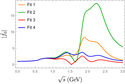
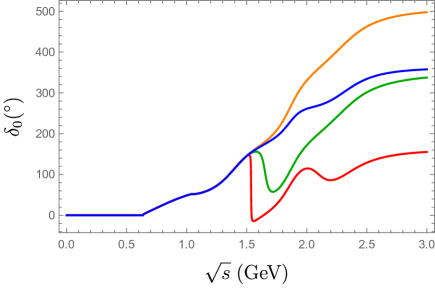
Figure 1: Modulus of the normalized scalar form factor $|\bar{f}_{0}|$ and its strong phase $\delta_{0}$ obtained from the four different fit scenarios of Ref. [31].

4.2 $B\to K\pi$ form factors for the $K\pi$ $S$-wave

We can generalise the above parametrization quite easily to the $B\to K\pi$ form factors with the $K\pi$ system in the $S$ wave. Specifically, for each $B\to K\pi$ form factor $F_{i}^{(\ell=0)}$ a two-component vector $\mathbf{F}_{i}$ is defined including the $B\to K\pi$ and $B\to K\eta^{\prime}$ form factors as components with $a=1$ and $a=2$. Following the previous discussion, we write

$$\mathbf{F}_{i}(s,q^{2})=\Omega(s)[{\bf 1}-V_{R}(s)\Sigma(s)]^{-1}N_{i}(s,q^{2})\equiv B(s)N_{i}(s,q^{2})\ ,$$ (37)

with the source term for a given form factor

$$N_{i,a}(s,q^{2})=\sum_{k=0}^{k_{\rm max}}d_{i,a}^{(k)}(q^{2})s^{k}-\sum_{r}g_{a}^{(r)}\frac{s-s_{K\eta}}{(s-\tilde{M}^{2}_{(r)})(s_{K\eta}-\tilde{M}^{2}_{(r)})}\beta_{i}^{(r)}(q^{2})\ .$$ (38)

Compared to our parametrisation for $P$-wave form factors with BW resonances in Ref. [12], and to the equivalent description given for the $S$ wave in Appendix B.1, we can see that there is an additional channel to be considered $(K\eta^{\prime})$ which doubles the number of parameters. Moreover, there is an additional polynomial term for each of the two channels, with an order which is not determined a priori. We constrain these parameters by assuming that $\mathbf{F}_{i}$ and $\mathbf{f}_{0}$ have the same phase for each channel, leading to the constraints ${\rm Im}[(BM)_{a}^{*}(BN_{i})_{a}]=0$ for $a=1,2$. One solution is provided by $N_{i,a}(s,q^{2})=\hat{\rho}_{i}(s,q^{2})M_{a}(s)$, leading to

$$F_{i}^{(\ell=0)}(s,q^{2})=\hat{\rho}_{i}(s,q^{2})f_{0}(s)\ .$$ (39)

We then further assume that the only $s$-dependence in $\hat{\rho}_{i}(s,q^{2})$ arises from kinematic effects. The latter can be identified, noticing that the alternative model with Breit-Wigner line shapes discussed in Appendix B.1 must feature similar kinematic structures. In particular, from Eq. (134), we expect the form factors $F_{0}^{(\ell=0)}$ and $F_{T}^{(\ell=0)}$ to have a kinematic factor $\sqrt{\lambda(s)}$ (coming from their definition in terms of $k_{0}^{\mu}$) which will not be present for $F_{t}$ and $F_{5}$. In addition, we may factor out the kinematic $q^{2}$ dependence to simplify the analysis of the sum rules. To this extent, we define

$$\hat{\omega}_{i}(s)\equiv\kappa_{i}(s,q^{2})\,{\omega}_{i}(s,q^{2})\ ,$$ (40)

where

$$\kappa_{0}(s,q^{2})=\frac{\sqrt{\lambda(s)}}{\sqrt{q^{2}}}\ ,\quad\kappa_{5,t}(s,q^{2})=\frac{2}{\sqrt{q^{2}}}\ ,\quad\kappa_{T}(s,q^{2})=\sqrt{\lambda(s)q^{2}}\ ,$$ (41)

such that the factors $\kappa_{i}(s,q^{2})$ cancel out the entire kinematic $s$ and $q^{2}$ dependence in $\omega_{i}(s,q^{2})$ defined in Eq. (32), leading to

$$\hat{\omega}\equiv\hat{\omega}_{0}=\hat{\omega}_{T}=\hat{\omega}_{5}=\hat{\omega}_{t}=\frac{3}{16\pi^{2}}\frac{\sqrt{\lambda_{K\pi}(s)}}{s}\ .$$ (42)

Taking into account these elements, we obtain

$$F_{i}^{(\ell=0)}(s,q^{2})=\kappa_{i}(s,q^{2})\,\rho_{i}(q^{2})\,f_{0}(s)\ ,$$ (43)

where $\rho_{i}(q^{2})$ is a real-valued function (independent of the channel $a$) that, by assumption, only depends on $q^{2}$. As a result, the sum rules given in Eq. (31) become constraints on the functions $\rho_{i}$,

$${\cal S}_{i}^{\rm OPE}(q^{2},s_{0},M^{2}) = \rho_{i}(q^{2})\int_{s_{\rm th}}^{s_{0}}ds\ e^{-s/M^{2}}(m_{K}^{2}-m_{\pi}^{2})\hat{\omega}(s)|f_{0}(s)|^{2}$$ (44)

$$\equiv \rho_{i}(q^{2})\;I_{\rm SR}(s_{0},M^{2})\ ,$$

where the integral $I_{\rm SR}$ only depends on $s_{0}$, $M^{2}$ and the form factor model for $f_{0}$. This leads to our final expression for the $S$-wave $B\to K\pi$ form factors,

$$F_{i}^{(\ell=0)}(s,q^{2})=\frac{\kappa_{i}(s,q^{2})f_{0}(s)\,{\cal S}_{i}^{\rm OPE}(q^{2},s_{0},M^{2})}{I_{\rm SR}(s_{0},M^{2})}\ ,\qquad i=\{0,t,5,T\}\ .$$ (45)

At this stage one could perform a $z$-expansion on both sides of the sum rules in Eq. (31), as done in Ref. [12]. Since the model for the form factors does not obey a simple parametrization in this variable, we refrain from doing so and work with Eq. (45) directly.

A comment is in order concerning the comparison with the $P$-wave case of Ref. [12], where both the $K\pi$ and $B\to K\pi$ form factors were modelled as a superposition of Breit-Wigner resonances with relative phases depending on $s$. The reality of the product of the $B\to K\pi$ form factors with the vector $K\pi$ form factor could be easily implemented there for each of the resonance contributions, by choosing the corresponding relative phase equal to that of the vector form factor. Here, we consider a rather different model for the $B\to K\pi$ scalar form factors, as the $s$-dependent phase is encoded in the overall matrix $B(s)$, together with the phase in the $K\eta^{\prime}$ channel and involving all resonances at once. Satisfying the reality constraint is therefore harder than in the $P$-wave case, which explains that a lesser number of parameters are fixed by the sum rules: only two per $B\to K\pi$ form factor in the scalar case, rather than two per $B\to K\pi$ form factor and per resonance in the vector case.

Parameter	Value	Ref	Parameter	Value	Ref
$m_{\pi^{\pm}}$	$140\,{\rm MeV}$	[16]	$m_{K^{\pm}}$	$494\,{\rm MeV}$	[16]
$m_{B^{0}}$	$5.28\,{\rm GeV}$	[16]	$f_{B}$	$207^{+17}_{-9}\,{\rm MeV}$	[48]
$\overline{m}_{b}(\overline{m}_{b})$	$4.18^{+0.03}_{-0.02}\,{\rm GeV}$	[16]	$\overline{m}_{c}(\overline{m}_{c})$	$1.27\pm 0.02\,{\rm GeV}$	[16]
$m_{s}(2\,\mbox{GeV})$	$93.4^{+8.6}_{-3.4}~{}\mbox{MeV}$	[16]	$m_{d}(2\,\mbox{GeV})$	$4.67^{+0.48}_{-0.17}~{}\mbox{MeV}$	[16]
$\lambda_{B}$	$460\pm 110\,{\rm MeV}$	[44]	$R$	$0.4^{+0.5}_{-0.3}$	[49]

Table 1: Compendium of input values used in the numerical analysis.

5 Numerical analysis

5.1 Numerical input

We follow the strategy outlined in Ref. [12] (see also Ref. [11] for further illustration). The inputs used in the numerical analysis and their sources are collected in Table 1. Despite the fact that the OPE for LCSRs is computed in HQET, the $b$-quark mass parameter still explicitly enters the LCSR for the heavy-light pseudoscalar current. We also need the $c$-quark mass for an estimate of nonlocal contributions in the analysis of $B\to K\pi\ell\ell$ decays. In both cases, we adopt typical $\overline{\rm MS}$ heavy quark masses, respectively: $\overline{m}_{b}=4.18\,{\rm GeV}$ and $\overline{m}_{c}=1.27\,{\rm GeV}$. The scale of the OPE is around $\mu=1\,{\rm GeV}$, hence we renormalize the $s$-quark mass value given in Table 1 to $\overline{m}_{s}(1\,{\rm GeV})=123(14)\,{\rm MeV}$.

Furthermore, we use the QCD sum rule estimate for the inverse moment $\lambda_{B}\equiv\lambda_{B}(1.0\,{\rm GeV})$ of the $B$-meson DA from Ref. [44], consistent with a more recent estimate of Ref. [45] obtained with the same method. This moment is the most important parameter determining the two- and three-particle $B$-meson DAs up to twist-four. For these DAs, we use the so-called “Model I” from Ref. [49] specified in Appendix B of Ref. [12], and based on the exponential model proposed originally in Ref. [46] (see also Ref. [24]). The only additional parameter needed in this model and within the adopted approximation of the light-cone OPE is the ratio $R=\lambda_{E}^{2}/\lambda_{H}^{2}$ of the two normalization parameters $\lambda_{E}$ and $\lambda_{H}$ determining the vacuum-to-$B$ matrix elements of the quark-antiquark-gluon HQET currents. The choice of $R$ is discussed in detail in Ref. [12]. For consistency, we also use the QCD sum rule result for the $B$-meson decay constant quoted in Table 1, which is close to (but less accurate than) the most recent lattice QCD average $f_{B}=190.0(1.3)$ MeV in Ref. [47].

For the $K\pi$ form factor, we use the four models obtained from the fits in Ref. [31]. The corresponding numerical values of the normalized form factor $\bar{f_{0}}(s)$ are presented in the ancillary files attached to this paper. For the normalization $f_{0}(0)$ in Eq. (36), we use $f_{0}(0)=f_{+}(0)=1.0$, which agrees with the analysis in Ref. [12] using the Belle data [42] on the $\tau\to K\pi\nu_{\tau}$ decay. For comparison, the current lattice QCD average at $N_{f}=2+1+1$ given in Ref. [47] is $f_{+}(0)=0.9698(17)$. We note that a different normalization would simply correspond to a rescaling of our form factors.

Following Ref. [12], we use the two-point QCD sum rule to fix the effective threshold parameter $s_{0}$ and the Borel mass squared $M^{2}$ appearing in the LCSRs. This sum rule and the procedure to fix $s_{0}$ and $M^{2}$ are described in Appendix C. As a result, we use the following values

$$s_{0}=1.8\;{\rm GeV}^{2}\ ,\quad M^{2}=1.25\;{\rm GeV}^{2}\ ,$$ (46)

independently of the $K\pi$ form factor model. These values satisfy the two-point sum rule for all such models, and at the same time, render the LCSRs well behaved. On the one hand, they lead to a reasonable convergence of the light-cone OPE, measured by the relative size of the contribution from three-particle DAs to the functions $S_{i}^{\text{OPE}}$ :

$$\frac{{\cal S}_{i,3p}^{\text{OPE}}}{{\cal S}_{i,2p}^{\text{OPE}}}<30\%\ ,$$ (47)

in the range $q^{2}=[0,6.0]\,{\rm GeV}^{2}$. On the other hand, the integral of the spectral density above the effective threshold is less than 40% of the total integral, sufficiently suppressing the sensitivity of the LCSRs to the quark-hadron duality approximation.

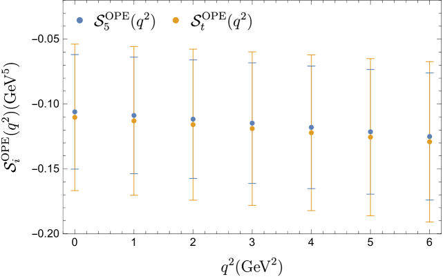
Figure 2: Comparison between the OPE contributions ${\cal S}_{5}^{\text{OPE}}$ and ${\cal S}_{t}^{\text{OPE}}$ as a function of $q^{2}$, for the values of $s_{0}$ and $M^{2}$ given in Eq. (46).

5.2 Results for $S$-wave $B\to K\pi$ form factors

Using the above inputs, we find the following central values for the integral $I_{\rm SR}$ defined in Eq. (44),

$$I_{\rm SR}(s_{0}=1.8\;{\rm GeV}^{2},M^{2}=1.25\;{\rm GeV}^{2})=\big{\{}6.9,\,9.7,\,5.3,\,8.4\big{\}}\cdot 10^{-3}\;{\rm GeV}^{4}\ ,$$ (48)

respectively from the fits $\{1,2,3,4\}$ for $f_{0}$, discussed in Section 4. Using these values, we can calculate the functions $\rho_{i}$, and hence determine the form factors $F_{i}^{(\ell=0)}(s,q^{2})$ from Eq. (45). We first comment on the numerical difference between ${\cal S}_{5}^{\text{OPE}}$ and ${\cal S}_{t}^{\text{OPE}}$ shown in Figure 2 for different values of $q^{2}$. Within uncertainties, the two OPE functions agree. Therefore, in what follows the numerical results for $i=5$ will not be used as they would lead to very similar results.

We also note that the functions ${\cal S}_{i}^{\text{OPE}}$ have a mild dependence on $q^{2}$ in the region of LCSR validity, yielding rather constant functions $\rho_{i}(q^{2})$. These functions are shown in Figure 3.

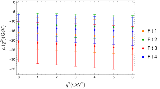
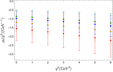
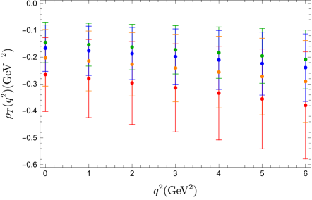
Figure 3: Results for the functions $\rho_{i}(q^{2})$ defined in Eq. (44) for all four fit models.

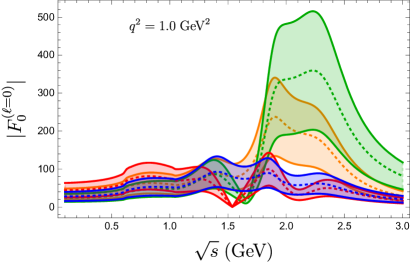
(a)

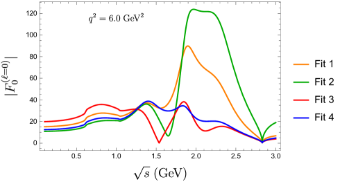
(b)

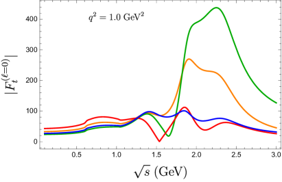
(c)

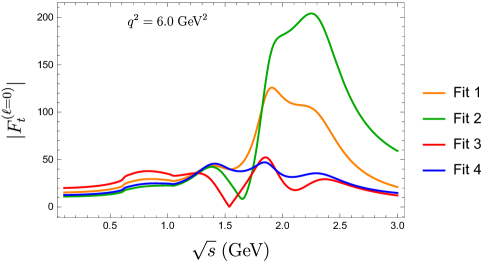
(d)

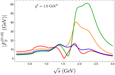
(e)

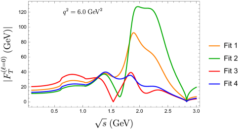
(f)

Figure 4: The form factors $F^{(\ell=0)}_{0},F_{t}^{(\ell=0)},F_{T}^{(\ell=0)}\equiv F_{0}^{T{(\ell=0)}}$ for the different fit models at $q^{2}=1.0\ \,{\rm GeV}^{2}$ (left) and $q^{2}=6.0\ \,{\rm GeV}^{2}$ (right).

In Figure 4, we present our results for the S-wave form factor $F_{0,t}^{(\ell=0)}$ and $F_{T}^{(\ell=0)}\equiv F_{0}^{T(\ell=0)}$ at $q^{2}=1.0$ and $6.0$ GeV² as a function of the $K\pi$ invariant mass $\sqrt{s}$. We display the uncertainties coming from the OPE calculation in Figure 4(a). For other values of $q^{2}$, as well as for the form factors $F_{t}^{(\ell=0)}$ and $F_{T}^{(\ell=0)}$, the corresponding uncertainties are in the same ballpark, hence we omit them in the other panels of Figure 4.

By definition, the $q^{2}$ dependence of the form factors in Eq. (45) is, apart from the factors $\kappa_{i}$, determined by $\mathcal{S}^{\rm OPE}_{i}$, which are parameterized by $\rho_{i}$. As the latter are rather constant functions of $q^{2}$, the resulting $q^{2}$ dependence of the form factors is almost entirely given by the kinematical factors $\kappa_{i}$. This is similar to the $P$-wave case discussed in terms of Breit-Wigner model in Ref. [12]. For completeness, we show the explicit $q^{2}$ dependence of the $B\to K\pi$ $S$-wave form factors in the next subsection, but we can already notice that these $B\to K\pi$ form factors strongly resemble the $K\pi$-form factor, revealing large deviations between different S-wave models for values of $s\gtrsim(1.8\,{\rm GeV})^{2}$.

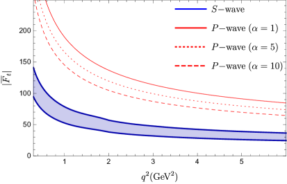
(a)

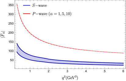
(b)

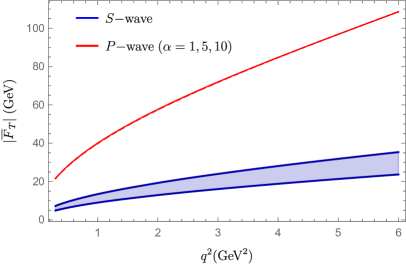
(c)

Figure 5: The $P$-wave form factors $F_{0,t,T}^{(\ell=1)}$ from Ref. [12] for $\alpha=1,~{}5$ and 10 compared to the $S$-wave form factors $F_{0,t,T}^{(\ell=0)}$ (we define $F_{T}^{(\ell=0,1)}\equiv F_{0}^{T(\ell=0,1)}$). The shaded bands indicate the full range of the $S$-wave models. The form factors are integrated over a $100$ MeV region around the $K^{*}(892)$ resonance: $(0.796\;{\rm GeV})^{2}<s<(0.996\;{\rm GeV})^{2}$.

5.3 Interplay of $S$- and $P$-wave form factors

We will combine our results with the $P$-wave $B\to K\pi$ form factors studied in Ref. [12] where the LCSRs were used to constrain the contributions of both $K^{*}(892)$ and $K^{*}(1410)$ $P$-wave resonances. In Ref. [12] a floating parameter $\alpha$ was introduced to vary the relative size of the $K^{*}(1410)$ contribution to the form factors, defined by

$${\cal F}_{K^{*}(1410)}(q^{2})=\alpha\,{\cal F}_{K^{*}(892)}(q^{2})\,.$$ (49)

Upper bounds on $\alpha$ were derived from LHCb measurements in the $K^{*}(1430)$ region in  Ref. [12]: the consideration of $P$-wave moments led to the bound $\alpha\lesssim 10$ whereas the branching ratio (neglecting $S$-wave contributions) led to $\alpha\lesssim 3$. We will show this in more detail later.

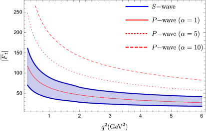
(a)

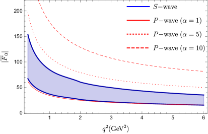
(b)

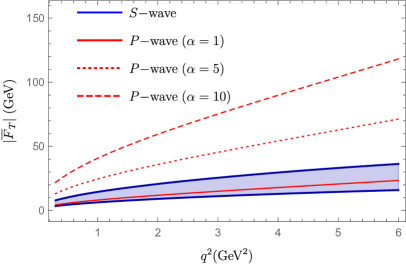
(c)

Figure 6: $P$- and $S$-wave form factors as in Figure 5, but in the higher $s$ region containing the resonances $K^{*}(1410)$ and $K^{*}_{0}(1430)$: $(1.33\;{\rm GeV})^{2}<s<(1.53\;{\rm GeV})^{2}$.

We consider the models for the $P$-wave form factors $F_{0,t,T}^{(\ell=1)}$ with $\alpha=1,5,10$ (we will focus on the case $\alpha=1$ later). In Figure 5 and Figure 6, they are compared to the corresponding $S$-wave form factors, for which the full range of variations between the different fit models is interpreted as a systematic uncertainty. In practice, the model 3 (model 4) always yields the lowest (highest) value for the $S$-wave form factor and we show the corresponding range of variation. We define normalized binned form factors through

$$\overline{F}_{0,t,T}^{(\ell)}(q^{2})=\frac{1}{s_{2}-s_{1}}\int\limits_{s_{1}}^{s_{2}}\!ds\,F_{0,t,T}^{(\ell)}(s,q^{2})\,~{}~{}~{}(\ell=0,1)\,.$$ (50)

In Figure 5 we show the normalized form factors by integrating the form factors in a $100\,{\rm MeV}$ bin  around the $K^{*}(892)$ resonance. We can see that the form factors $F_{0,t,T}^{(\ell=0)}$ and $F_{0,t,T}^{(\ell=1)}$ have a similar $q^{2}$ dependence, while the magnitude of each form factor depends on the specific $S$-wave model or on the value of $\alpha$ in the $P$-wave case. For $F_{0}$ and $F_{T}$, the variation of $\alpha$ has only a tiny effect, indistinguishable in the plots. As expected, the magnitudes of the $S$-wave form factors, though noticeable in this region, are smaller than their $P$-wave counterparts. We add that the $F_{t}$ form factor does not contribute to $B\to K^{*}\ell\ell$ in the limit of massless leptons, but this form factor plays an important role in non-leptonic decays [18, 19, 20, 21].

In Figure 6, the same comparison is shown for the region $1.33<\sqrt{s}<1.53$ GeV, which is dominated by the $P$-wave resonance $K^{*}(1410)$ and the $S$-wave resonance $K^{*}(1430)$. As expected, varying $\alpha$ has a much more significant impact on the $P$-wave model in this region. The interplay between the $P$ and $S$ waves in the $B\to K\pi$ form factors is also more substantial, so that both partial waves contribute at the same level, (and they are very close numerically for $\alpha\simeq 1$).

6 Application to the $B\to K\pi\ell\ell$ decay

In Ref. [12], we applied LCSRs to the $B\to K\pi\ell\ell$ decay with the $K\pi$ system in the $P$ wave. We are now in a position to extend this analysis by adding the $S$-wave contribution. The discussion is aimed at clarifying two different issues: the pollution from the $S$-wave component under the $K^{*}(892)$ peak, and the exploitation of the LHCb measurements in the $K^{*}(1410)$ region. Before discussing a few applications, we will recall elements already presented in Ref. [12], adapting them to include the $S$ wave.

6.1 Formalism

The amplitude ${\cal A}\equiv{\cal A}(\bar{B}^{0}\to K^{-}(k_{1})\pi^{+}(k_{2})\ell^{-}(q_{1})\ell^{+}(q_{2}))$ is given by:

$$i{\cal A}=g_{F}\frac{\alpha}{4\pi}\bigg{[}(C_{9}\,L_{V\mu}+C_{10}\,L_{A\mu})\ {\cal F}_{L}^{\mu}+\frac{L_{V\mu}}{q^{2}}\Big{\{}2m_{b}C_{7}\,{\cal F}^{T\mu}_{R}-i\,16\pi^{2}\,{\cal H}^{\mu}\Big{\}}\bigg{]}$$ (51)

with $g_{F}\equiv 4G_{F}/\sqrt{2}\,V^{*}_{ts}V_{tb}$, $L_{V(A)}^{\mu}\equiv\bar{u}_{\ell}(q_{1})\gamma^{\mu}(\gamma_{5})v_{\ell}(q_{2})$, and the local and non-local hadronic matrix elements:

$${\cal F}_{L}^{\mu} \equiv i\,\langle K^{-}(k_{1})\pi^{+}(k_{2})|\bar{s}\gamma^{\mu}P_{L}\,b|\bar{B}^{0}(p)\rangle=\frac{1}{2}\big{(}F_{\perp}\,k_{\perp}^{\mu}+F_{\|}\,k_{\|}^{\mu}+F_{0}\,k_{0}^{\mu}+F_{t}\,k_{t}^{\mu}\big{)}\ ,$$ (52)

$${\cal F}^{T\mu}_{R} \equiv \langle K^{-}(k_{1})\pi^{+}(k_{2})|\bar{s}\sigma^{\mu\nu}q_{\nu}P_{R}\,b|\bar{B}^{0}(p)\rangle=\frac{1}{2}\big{(}F^{T}_{\perp}\,k_{\perp}^{\mu}+F^{T}_{\|}\,k_{\|}^{\mu}+F^{T}_{0}\,k_{0}^{\mu}\big{)}\ ,$$ (53)

$${\cal H}^{\mu} \equiv i\int dx\,e^{i\,q\cdot x}\langle K^{-}(k_{1})\pi^{+}(k_{2})|T\{j_{\rm em}^{\mu}(x)\,\mathcal{O}_{\rm 4q}(0)\}|\bar{B}^{0}(p)\rangle={\cal H}_{\perp}k_{\perp}^{\mu}+{\cal H}_{\|}k_{\|}^{\mu}+{\cal H}_{0}\,k_{0}^{\mu}\ ,\ \quad$$ (54)

with $q=q_{1}+q_{2}$ and $p=q+k$. In addition to the form factors $F^{(T)}_{i}$, the decay amplitude involves the functions ${\cal H}_{i}(k^{2},q^{2},q\cdot\bar{k})$ describing the non-local effects which appear when the lepton pair couples to the electromagnetic current, through a penguin contraction of the four-quark operators $\mathcal{O}_{\rm 4q}\sim\bar{s}b\bar{q}q$.

We define the decomposition in terms of transversity amplitudes ${\cal A}^{L,R}_{i}$ :

$$i{\cal A}=\frac{\alpha\,g_{F}}{8\pi{\cal N}}\bigg{\{}L_{\mu}\big{(}{\cal A}^{L}_{\perp}\,k_{\perp}^{\mu}+{\cal A}^{L}_{\|}\,k_{\|}^{\mu}+{\cal A}^{L}_{0}\,k_{0}^{\mu}+{\cal A}^{L}_{t}\,k_{t}^{\mu}\big{)}+R_{\mu}\big{(}{\cal A}^{R}_{\perp}\,k_{\perp}^{\mu}+{\cal A}^{R}_{\|}\,k_{\|}^{\mu}+{\cal A}^{R}_{0}\,k_{0}^{\mu}+{\cal A}^{R}_{t}\,k_{t}^{\mu}\big{)}\bigg{\}}\ ,$$ (55)

where $L^{\mu}\equiv\bar{u}_{\ell}(q_{1})\,\gamma^{\mu}P_{L}\,v_{\ell}(q_{2})$ and $R^{\mu}\equiv\bar{u}_{\ell}(q_{1})\,\gamma^{\mu}P_{R}\,v_{\ell}(q_{2})$, and $P_{L,R}=(1\mp\gamma_{5})/2$ are the left- and right-chirality components of the lepton current. The normalization constant $N$ is set to the value

$${\cal N}=\alpha G_{F}V_{tb}V_{ts}^{*}\sqrt{\frac{\sqrt{\lambda\lambda_{K\pi}\lambda_{q}}}{3\cdot 2^{13}\pi^{7}m_{B}^{3}\,k^{2}}}\,,$$ (56)

for easier comparison with the $P$-wave results in the narrow-width limit for the $K^{*}$ meson [12].

Comparing with Eq. (51) one can see that

$${\cal A}_{i}^{L,R}={\cal N}\bigg{[}(C_{9}\mp C_{10})F_{i}+\frac{2m_{b}}{q^{2}}\Big{\{}C_{7}F_{i}^{T}-i\frac{16\pi^{2}}{m_{b}}{\cal H}_{i}\Big{\}}\bigg{]}\ ,\quad i=\{\perp,\|,0,t\}\ ,$$ (57)

keeping in mind that ${\cal A}_{i}^{L,R}\equiv{\cal A}_{i}^{L,R}(k^{2},q^{2},q\cdot\bar{k})$, etc. For ${\cal A}_{t}^{L,R}$ only the first term is present due to $F_{t}^{T}={\cal H}_{t}=0$. In addition, since we consider two leptons of equal masses, one has $L_{\mu}k_{t}^{\mu}=-R_{\mu}k_{t}^{\mu}$ and the timelike-helicity amplitude depends only on the $C_{9}$ - independent combination ${\cal A}_{t}\equiv{\cal A}_{t}^{L}-{\cal A}_{t}^{R}$.

Concerning the non-local form factors ${\cal H}_{i}$, we will use the operator product expansion (OPE) at leading power, which allows us to express the functions ${\cal H}_{i}$ in terms of the local form factors. Using the notation of Ref. [50], we have

$${\cal H}_{i}(k^{2},q^{2},q\cdot\bar{k})=\frac{i\,q^{2}}{32\pi^{2}}\Delta C_{9}(q^{2})F_{i}(k^{2},q^{2},q\cdot\bar{k})+\mathcal{O}(\alpha_{s})+\cdots$$ (58)

where the ellipses denote higher OPE contributions, and the function $\Delta C_{9}(q^{2})$ is given by

$$\Delta C_{9}(q^{2})=\frac{4}{9}(C_{F}C_{1}+C_{2})\bigg{[}\frac{2}{3}+\frac{4m_{c}^{2}}{q^{2}}-\log\frac{m_{c}^{2}}{m_{b}^{2}}-\bigg{(}2+\frac{4m_{c}^{2}}{q^{2}}\bigg{)}\sqrt{\frac{4m_{c}^{2}-q^{2}}{q^{2}}}\arctan\sqrt{\frac{q^{2}}{4m_{c}^{2}-q^{2}}}\bigg{]}\,,$$ (59)

keeping only the leading contributions from the current-current $(\bar{s}c)(\bar{c}b)$ operators. The definitions used here are the same as in Ref. [50], where $C_{1}(m_{b})\simeq-0.29$ and $C_{2}(m_{b})\simeq 1.01$. The resulting transversity amplitudes in this approximation are given by

$${\cal A}_{i}^{L,R}={\cal N}\bigg{[}\big{(}C_{9}+\Delta C_{9}(q^{2})\mp C_{10}\big{)}F_{i}+\frac{2m_{b}}{q^{2}}C_{7}F_{i}^{T}\bigg{]}\ ,\quad i=\{\perp,\|,0,t\}\ .$$ (60)

For the numerical inputs, we use $C_{9}(m_{b})=4.3$, $C_{10}(m_{b})=-4.2$, $C_{7}^{\rm eff}(m_{b})=-0.3$ and $\alpha_{\rm em}(m_{b})=1/129$ (see e.g. Ref. [51]). The transversity amplitudes ${\cal A}_{i}^{L,R}$ in Eq. (60) can be expanded in partial waves ${\cal A}_{i}^{L,R(\ell)}(k^{2},q^{2})$ in the same way as the form factors. The form factors $F_{0,t}$ contain the $S$-wave, as described in Eq. (5), whereas $F_{\perp,\|}$ start at the $P$-wave only (see Ref. [12] for their partial-wave expansion).

Following the same steps as in Ref. [12] and considering the decay chain $B\to V^{*}(\to\ell\ell)K\pi$, we may rewrite the amplitude ${\cal A}$ in terms of the helicity amplitudes $H_{\lambda}^{L,R}$:

$$i{\cal A}=\frac{\alpha g_{F}}{8\pi{\mathcal{N}}}\sum_{\lambda}g_{\lambda\lambda}[(\epsilon_{\lambda}\cdot L)\ H^{L}_{\lambda}+(\epsilon_{\lambda}\cdot R)\ H^{R}_{\lambda}]\ ,$$ (61)

with $\lambda=\{0,t,+,-\}$ and $g_{tt}=1$, $g_{00}=g_{++}=g_{--}=-1$. The polarisations of the virtual intermediate gauge boson $V^{*}$ defined in the $B$-meson rest frame are

$$\epsilon_{\pm}^{\mu}=(0,1,\mp i,0)/\sqrt{2}\quad\epsilon_{0}^{\mu}=(-q_{z},0,0,-q_{0})/\sqrt{q^{2}}\quad\epsilon_{t}^{\mu}=(q_{0},0,0,q_{z})/\sqrt{q^{2}}\ ,$$ (62)

where $q^{\mu}=(q_{0},0,0,q_{z})$. We can then define transversity amplitudes, performing the partial-wave expansion up to the $P$-wave:

$$H_{+}^{L,R} =\sqrt{3}\,\frac{\widehat{A}_{\|}^{L,R}+\widehat{A}_{\perp}^{L,R}}{\sqrt{2}}(-\sin\theta_{K})+\cdots\ , H_{-}^{L,R} =\sqrt{3}\,\frac{\widehat{A}_{\|}^{L,R}-\widehat{A}_{\perp}^{L,R}}{\sqrt{2}}(-\sin\theta_{K})+\cdots\ ,$$ (63)

$$H_{0}^{L,R} =\sqrt{2}(\widehat{S}_{0}^{L,R}+\sqrt{3}\widehat{A}_{0}^{L,R}\cos\theta_{K}+\cdots)\ , H_{t} =-\sqrt{2}(\widehat{S}_{t}+\sqrt{3}\widehat{A}_{t}\cos\theta_{K}+\cdots)\ ,$$ (64)

with $H_{t}\equiv H_{t}^{L}-H_{t}^{R}$. Here $\widehat{S}^{L,R}_{i}$ and $\widehat{A}^{L,R}_{i}$ denote  the amplitudes with $\ell_{K\pi}=0$ and $\ell_{K\pi}=1$ respectively, and the ellipsis indicates the $D$-wave as well as higher partial waves. The amplitudes entering Eqs. (63) and (64) are related to the transversity amplitudes introduced in Eq. (55):

$$\widehat{A}_{\perp}^{L,R} =-\frac{\sqrt{\lambda_{K\pi}}}{k^{2}}{\cal A}_{\perp}^{L,R(1)}\ , \widehat{A}_{\|}^{L,R} =\frac{\sqrt{\lambda_{K\pi}}}{k^{2}}{\cal A}_{\|}^{L,R(1)}\ ,$$

$$\widehat{A}_{0}^{L,R} =-{\cal A}_{0}^{L,R(1)}/\sqrt{2}\ , \widehat{A}_{t} =-{\cal A}_{t}^{(1)}/\sqrt{2}\ ,$$

$$\widehat{S}_{0}^{L,R} =-{\cal A}_{0}^{L,R(0)}/\sqrt{2}\ , \widehat{S}_{t} =-{\cal A}_{t}^{(0)}/\sqrt{2}\ ,$$ (65)

where the first two lines were already shown in Ref. [12], but the last line is new, following from our consideration of $S$-wave contributions.

6.2 Differential decay rate

The differential decay rate for $\bar{B}\to K^{-}\pi^{+}\ell\ell$ is given by

$$\frac{d\Gamma}{dq^{2}\,ds\,d\cos\theta_{\ell}\,d\cos\theta_{K}\,d\phi}=\frac{1}{2^{15}\pi^{6}m_{B}}\frac{\sqrt{\lambda\lambda_{q}\lambda_{K\pi}}}{m_{B}^{2}q^{2}s}\sum_{s_{1},s_{2}}|{\cal A}|^{2}\ ,$$ (66)

where $s=k^{2}$ and $\lambda_{q}\equiv\lambda(q^{2},m_{\ell}^{2},m_{\ell}^{2})$. According to Eq. (61), $|{\cal A}|^{2}$ involves the products of the hadronic amplitudes $\widehat{A}_{i}^{L,R}$ (known in terms of the form factors $F_{i},F_{i}^{T}$ and non-local contributions neglected here) and the leptonic amplitudes $L_{\lambda}$ and $R_{\lambda}$ (which can be easily evaluated in the $B$-meson rest frame). Summing over the spins of the outgoing leptons yields the final expression:

$$\frac{d\Gamma}{dq^{2}\,ds\,d\cos\theta_{\ell}\,d\cos\theta_{K}\,d\phi}=\frac{9}{32\pi}\bar{I}(q^{2},s,\theta_{\ell},\theta_{K},\phi)\,,$$ (67)

containing the following decomposition in terms of angular observables:

$$\bar{I}(q^{2},s,\theta_{\ell},\theta_{K},\phi) =\bar{I}_{1}^{s}\sin^{2}\theta_{K}+\bar{I}_{1}^{c}\cos^{2}\theta_{K}+(\bar{I}_{2}^{s}\sin^{2}\theta_{K}+\bar{I}_{2}^{c}\cos^{2}\theta_{K})\cos 2\theta_{\ell}$$

$$+\bar{I}_{3}\sin^{2}\theta_{K}\sin^{2}\theta_{\ell}\cos 2\phi+\bar{I}_{4}\sin 2\theta_{K}\sin 2\theta_{\ell}\cos\phi$$

$$-\bar{I}_{5}\sin 2\theta_{K}\sin\theta_{\ell}\cos\phi$$

$$-(\bar{I}_{6}^{s}\sin^{2}\theta_{K}+{\bar{I}_{6}^{c}\cos^{2}\theta_{K}})\cos\theta_{\ell}+\bar{I}_{7}\sin 2\theta_{K}\sin\theta_{\ell}\sin\phi$$

$$-\bar{I}_{8}\sin 2\theta_{K}\sin 2\theta_{\ell}\sin\phi-\bar{I}_{9}\sin^{2}\theta_{K}\sin^{2}\theta_{\ell}\sin 2\phi$$

$$+\bar{\tilde{I}}_{1b}^{c}\cos(\theta_{K})+\bar{\tilde{I}}_{2b}^{c}\cos(\theta_{K})\cos(2\theta_{\ell})$$

$$+\bar{\tilde{I}}_{4}\sin(\theta_{K})\sin(2\theta_{\ell})\cos(\phi)-\bar{\tilde{I}}_{5}\sin(\theta_{K})\sin(\theta_{\ell})\cos(\phi)$$

$$+\bar{\tilde{I}}_{7}\sin(\theta_{K})\sin(\theta_{\ell})\sin(\phi)-\bar{\tilde{I}}_{8}\sin(\theta_{K})\sin(2\theta_{\ell})\sin(\phi)\,.$$ (68)

The expressions for the angular observables in which the contributions of the $S$ and $P$ waves are separated are :

$$\bar{I}_{1}^{s} =\frac{(2+\beta_{\ell}^{2})}{4}\left[|\widehat{A}_{\perp}^{L}|^{2}+|\widehat{A}_{\parallel}^{L}|^{2}+(L\to R)\right]+\frac{4m_{\ell}^{2}}{q^{2}}{\rm Re}(\widehat{A}_{\perp}^{L}(\widehat{A}_{\perp}^{R})^{*}+\widehat{A}_{\parallel}^{L}(\widehat{A}_{\parallel}^{R})^{*})$$

$$\qquad+\frac{1}{3}\left[|\widehat{S}_{0}^{L}|^{2}+(L\to R)+(1-\beta_{\ell}^{2})(|\widehat{S}_{t}|^{2}+2{\rm Re}(\widehat{S}_{0}^{L}(\widehat{S}_{0}^{R})^{*})\right],$$ (69)

$$\bar{I}_{1}^{c} =|\widehat{A}_{0}^{L}|^{2}+|\widehat{A}_{0}^{R}|^{2}+\frac{4m_{\ell}^{2}}{q^{2}}\left[|\widehat{A}_{t}|^{2}+2{\rm Re}(\widehat{A}_{0}^{L}(\widehat{A}_{0}^{R})^{*})\right]$$

$$\qquad+\frac{1}{3}\left[|\widehat{S}_{0}^{L}|^{2}+(L\to R)+(1-\beta_{\ell}^{2})(|\widehat{S}_{t}|^{2}+2{\rm Re}(\widehat{S}_{0}^{L}(\widehat{S}_{0}^{R})^{*})\right],$$ (70)

$$\bar{I}_{2}^{s} =\frac{\beta_{\ell}^{2}}{4}\left[|\widehat{A}_{\perp}^{L}|^{2}+|\widehat{A}_{\parallel}^{L}|^{2}+(L\to R)\right]-\frac{1}{3}\beta_{\ell}^{2}\left[|\widehat{S}_{0}^{L}|^{2}+(L\to R)\right],$$ (71)

$$\bar{I}_{2}^{c} =-\beta_{\ell}^{2}\left[|\widehat{A}_{0}^{L}|^{2}+(L\to R)\right]-\frac{1}{3}\beta_{\ell}^{2}\left[|\widehat{S}_{0}^{L}|^{2}+(L\to R)\right],$$ (72)

$$\bar{I}_{3} =\frac{1}{2}\beta_{\ell}^{2}\left[|\widehat{A}_{\perp}^{L}|^{2}-|\widehat{A}_{\parallel}^{L}|^{2}+(L\to R)\right],$$ (73)

$$\bar{I}_{4} =\frac{1}{\sqrt{2}}\beta_{\ell}^{2}\left[{\rm Re}(\widehat{A}_{0}^{L}(\widehat{A}_{\parallel}^{L})^{*})+(L\to R)\right],$$ (74)

$$\bar{I}_{5} =\sqrt{2}\beta_{\ell}\left[{\rm Re}(\widehat{A}_{0}^{L}(\widehat{A}_{\perp}^{L})^{*})-(L\to R)\right],$$ (75)

$$\bar{I}_{6}^{s} =2\beta_{\ell}\left[{\rm Re}(\widehat{A}_{\parallel}^{L}(\widehat{A}_{\perp}^{L})^{*})-(L\to R)\right],$$ (76)

$$\bar{I}_{6}^{c} =0,$$ (77)

$$\bar{I}_{7} =\sqrt{2}\beta_{\ell}\left[{\rm Im}(\widehat{A}_{0}^{L}(\widehat{A}_{\parallel}^{L})^{*})-(L\to R)\right],$$ (78)

$$\bar{I}_{8} =\frac{1}{\sqrt{2}}\beta_{\ell}^{2}\left[{\rm Im}(\widehat{A}_{0}^{L}(\widehat{A}_{\perp}^{L})^{*})+(L\to R)\right],$$ (79)

$$\bar{I}_{9} =\beta_{\ell}^{2}\left[{\rm Im}(\widehat{A}_{\perp}^{L}(\widehat{A}_{\parallel}^{L})^{*})+(L\to R)\right]\,,$$ (80)

with $\beta_{\ell}=\sqrt{\lambda_{q}}/q^{4}=\sqrt{1-4m_{\ell}^{2}/q^{2}}$. The angular observables containing interferences between the $S$ and $P$-waves are:

$$\bar{\tilde{I}}_{1b}^{c} =\frac{2}{3}\sqrt{3}{\rm Re}\left[\widehat{S}_{0}^{L}(\widehat{A}_{0}^{L})^{*}+(L\to R)+(1-\beta_{\ell}^{2})(\widehat{S}_{0}^{L}(\widehat{A}_{0}^{R})^{*}+\widehat{S}_{0}^{R}(\widehat{A}_{0}^{L})^{*}+\widehat{S}_{t}\widehat{A}_{t}^{*})\right],$$ (81)

$$\bar{\tilde{I}}_{2b}^{c} =-\frac{2}{3}\sqrt{3}\beta_{\ell}^{2}{\rm Re}\left[\widehat{S}_{0}^{L}(\widehat{A}_{0}^{L})^{*}(L\to R)\right],$$ (82)

$$\bar{\tilde{I}}_{4} =\frac{2}{3}\sqrt{\frac{3}{2}}\beta_{\ell}^{2}{\rm Re}\left[\widehat{S}_{0}^{L}(\widehat{A}_{\parallel}^{L})^{*}+(L\to R)\right],$$ (83)

$$\bar{\tilde{I}}_{5} =\frac{4}{3}\sqrt{\frac{3}{2}}\beta_{\ell}{\rm Re}\left[\widehat{S}_{0}^{L}(\widehat{A}_{\perp}^{L})^{*}-(L\to R)\right],$$ (84)

$$\bar{\tilde{I}}_{7} =\frac{4}{3}\sqrt{\frac{3}{2}}\beta_{\ell}{\rm Im}\left[\widehat{S}_{0}^{L}(\widehat{A}_{\parallel}^{L})^{*}-(L\to R)\right],$$ (85)

$$\bar{\tilde{I}}_{8} =\frac{2}{3}\sqrt{\frac{3}{2}}\beta_{\ell}^{2}{\rm Im}\left[\widehat{S}_{0}^{L}(\widehat{A}_{\perp}^{L})^{*}+(L\to R)\right]\,.$$ (86)

As already indicated in Ref. [12], the choice of normalisation in Eq. (56) yields a very simple expression for Eq. (67). If we neglect $S$-wave contributions, setting $\widehat{S}_{0}^{L,R}=\widehat{S}_{t}=0$, we can see that $\bar{I}$ is formally the same expression as the one obtained in Eqs (3.10) and (3.21) of Ref. [52], with the angular coefficients $\bar{I}_{1s,1c,2s,2c,3,4,5,6s,6c,7,8,9}$ given by Eqs. (3.34)-(3.45) of the same reference, as long as the transversity amplitudes $A_{i}$ of Eqs. (3.28)-(3.31) in Ref. [52] are replaced by the transversity amplitudes $\widehat{A}_{i}$ given in Eq. (65). We also agree with the structure of the differential decay rate in terms of transversity amplitudes given in Ref. [17] for the terms involving the $S$ wave.

6.3 Predictions for the differential rate in the $K^{*}(892)$ region

We start by considering the case where the $K\pi$ invariant mass is close to the $K^{*}(892)$ $P$-wave resonance. At such low invariant masses, the $S$ and $P$ waves are dominant and one can neglect higher partial waves. The differential rate, integrated over all angles, is then

$$\frac{d\Gamma}{dq^{2}ds}=|\widehat{S}^{L}|^{2}+|\widehat{S}^{R}|^{2}+|\widehat{A}_{\|}^{L}|^{2}+|\widehat{A}_{\|}^{R}|^{2}+|\widehat{A}_{\perp}^{L}|^{2}+|\widehat{A}_{\perp}^{R}|^{2}+|\widehat{A}_{0}^{L}|^{2}+|\widehat{A}_{0}^{R}|^{2}\,.$$ (87)

We note that the $F_{t}^{{(\ell=0,1)}}$ form factors do not enter because we are assuming massless leptons.

In Ref. [14], the LHCb collaboration presented measurements of the $B\to K\pi\mu\mu$ differential decay rate in the $K^{*}(892)$ region. To quantify the $S$-wave contribution, they also measured the $S$-wave fraction in several $q^{2}$ bins and in two different ranges of the $K\pi$ invariant mass around the $K^{*}$ resonance. In analogy with the expression of $F_{S}$ in Eq. (5) of Ref. [14], we define:

$$F_{S}\equiv\frac{\int_{\text{bin}}ds\,(|\widehat{S}^{L}|^{2}+|\widehat{S}^{R}|^{2})}{\int_{\text{bin}}ds\,(|\widehat{S}^{L}|^{2}+|\widehat{S}^{R}|^{2}+|\widehat{A}_{\|}^{L}|^{2}+|\widehat{A}_{\|}^{R}|^{2}+|\widehat{A}_{\perp}^{L}|^{2}+|\widehat{A}_{\perp}^{R}|^{2}+|\widehat{A}_{0}^{L}|^{2}+|\widehat{A}_{0}^{R}|^{2})}\,,$$ (88)

and we compute this fraction in

$${\rm bin\;1}: \quad\quad(0.796\;{\rm GeV})^{2}<s<(0.996\;{\rm GeV})^{2}\,,$$ (89)

$${\rm bin\;2}: \quad\quad(0.644\;{\rm GeV})^{2}<s<(1.200\;{\rm GeV})^{2}\,.$$ (90)

Our results for both bins are presented in Figure 7, using the $P$-wave model of Ref. [12] for $\alpha=1$, compared with the LHCb data from Ref. [14]. We predict a rather small $S$-wave contribution in this region, in agreement with some of the LHCb data points. It would be very difficult to achieve a full agreement, as the data features very rapid changes in $F_{S}$ as $q^{2}$ varies. Since this observable is driven by form factors with a monotonous $q^{2}$ behavior, we cannot propose any plausible theoretical explanation for such rapid variations.

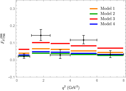
(a)

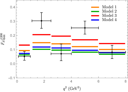
(b)

Figure 7: $S$-wave fration $F_{S}$ in bin 1 (left) and bin 2 (right) for different $q^{2}$ bins compared with the LHCb data points from Ref. [14].

The LHCb collaboration then presented a measurement of the $B\to K^{*}\ell\ell$ branching ratio by subtracting the $S$-wave contribution $F_{S}$ from the data. In Figure 8, we compare this experimental data with our predictions for the branching ratio restricted to the $P$-wave component, calculated at various values of $\alpha$ in the region $(0.796\;{\rm GeV})^{2}<s<(0.996\;{\rm GeV})^{2}$ and in different $q^{2}$ bins. We normalize the branching ratio to the $q^{2}$-bin size in the same way as in the experimental analysis:

$$\frac{dB}{dq^{2}}=\frac{1}{q_{2}^{2}-q_{1}^{2}}\int_{q_{1}^{2}}^{q_{2}^{2}}dq^{2}\int_{s_{\rm min}}^{s_{\rm max}}ds\;\tau_{B}\;\frac{d\Gamma}{dq^{2}ds}\ .$$ (91)

We observe that higher values of $\alpha$ push down the predictions for the branching ratios in the $K^{*}(892)$ region, while lower values push them up. From now on, we will set $\alpha=1$ for the $P$-wave contribution, as it yields a good agreement with the LHCb measurements of the branching ratios.

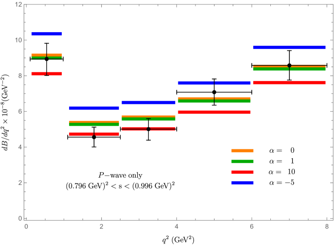
(a)

Figure 8: Theory predictions for the $B\to(K\pi)_{P}\ell^{+}\ell^{-}$ branching ratio within the $K\pi$ invariant mass bin $(0.796\;{\rm GeV})^{2}<s<(0.996\;{\rm GeV})^{2}$, for different values of $\alpha$, compared to the LHCb measurements of $B\to K^{*}\mu^{+}\mu^{-}$ in Ref. [14].

Finally, we note that our results could allow us to predict angular observables associated with different moments of the $S$-wave contribution in the $K^{*}(892)$ region [15, 17]. Comparing such predictions with data could thus give more insight into the dynamics of the $S$-wave component. However, we are not aware of corresponding experimental data on the $S$-wave in this region. The $S$-wave contribution has been discussed for branching ratios [14] but it was treated as a nuisance parameter in the context of angular moments  [3]. We will thus leave this study for further work, focusing on the $K^{*}(1410)$ and $K^{*}_{0}(1430)$ region from now on.

6.4 Differential decay rate in the $K^{*}(1410)$ and $K^{*}_{0}(1430)$ region

The LHCb collaboration also measured the $B\to K\pi\mu\mu$ differential decay rate in the region $(1.33\;{\rm GeV})^{2}<s<(1.52\;\rm{GeV})^{2}$ and in different $q^{2}$ bins in Ref. [13]. Taking Eq. (87), we compute this rate using the four different $S$-wave models and with different values of $\alpha$ for the $P$-wave contribution. The $S$-wave is substantially more important here than in the $K^{*}(892)$ region. In Figure 9, we show our results considering only the $S$-wave contribution for the four different models (normalized following Eq. (91)). We see that in the higher $q^{2}$ bins, some of the models yield already too large value compared to the data, even before including the (positive) $P$-wave contribution. Moreover the sum of the $S$- and $P$-wave contributions to the branching ratios should be smaller than the experimental value, since the latter also includes a (positive) contribution of the $D$ wave that we are not able to estimate at this stage, but which is not necessarily negligible [13].

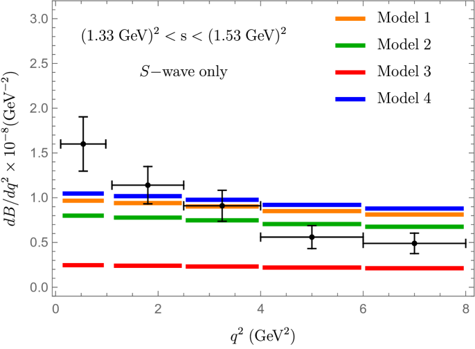
(a)

Figure 9: LHCb data and the $S$-wave only contribution to the differential rate in different $q^{2}$ bins integrated over $s$ in the high bin.

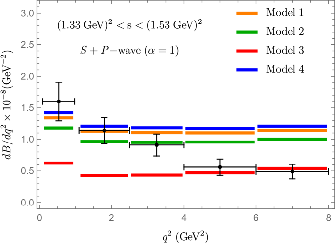
(a)

Figure 10: LHCb data and $P$ ($\alpha=1$) and $S$-wave contributions to the differential rate in different $q^{2}$ bins integrated over $s$ in the high bin.

Adding the $P$-wave (with $\alpha=1$) gives the predictions shown in Figure 10. We observe good agreement for the lower $q^{2}$ bins. At larger $q^{2}$, we cannot reproduce the measured $q^{2}$ dependence, as our result combines the increasing $P$-wave contribution with an almost constant $S$-wave contribution (for all four models).

It seems difficult to improve the situation significantly by changing the parameter $\alpha$ of the $P$-wave contribution. Indeed, this $P$-wave contribution is responsible for the satisfactory agreement for the $B\to K\pi\ell\ell$ branching ratio at low $q^{2}$ in the two regions of $K\pi$ invariant mass that we have considered here.

The $D$-wave contribution constitutes a possible missing element. It is not included in our analysis but would yield a further positive contribution to the branching ratio. This contribution might change the $q^{2}$-dependence of the branching ratio, but at the same time, it will increase the overall prediction and thus worsen the agreement with the data.

We thus expect that the origin of the disagreement encountered with data at large $q^{2}$ might be related to the overall normalisation and the $q^{2}$-dependence of the $S$-wave contribution around the scalar resonance $K^{*}_{0}(1430)$. At this stage, one should remember that the four versions of the $B\to K\pi$ $S$-wave form factors adopted here originate from the models for the scalar $K\pi$ form factor of Ref. [31]. These versions were not meant to exhaust all the possible models for this form factor, but rather to show the possible range of variation at intermediate $K\pi$ invariant mass allowed by the dispersive approach and the limited amount of data available to fix the free parameters of the models. The description of the $K\pi$ scalar form factor, and consequently, of the models for the $B\to K\pi$ $S$-wave form factors, can certainly be explored further, in particular, concerning the impact of the so-called source term (the polynomial terms describing the high-energy behaviour), and the presence of additional resonances around 2 GeV. Therefore, one should interpret the fact that we get only a partial agreement with the data (although in the right ballpark regarding the prediction for the branching ratio) as the indication that the $S$-wave models considered here may serve as a good starting point requiring further tuning. This in turn could yield a larger range of possibilities regarding the contribution from the $K^{*}_{0}(1430)$, which is fairly similar in the models 1,2,3 (see Figure 1), leading to rather close predictions for the branching ratio (see Figure 10). We will refrain from entering such an investigation here, as we want mainly to highlight the possibilities given by our framework.

6.5 Angular observables in the $K^{*}(1410)$ and $K^{*}_{0}(1430)$ region

We can now turn to the analysis of angular observables performed in Ref. [12] and extend it to include the $S$ wave. In Ref. [13] the LHCb experiment has analysed the moments $\Gamma_{i}$ ($i=1\ldots 41$) of the angular distribution of $B\to K\pi\mu^{+}\mu^{-}$ in the region of $K\pi$ and dilepton invariant masses $\sqrt{k^{2}}\in[1.33,1.53]\,{\rm GeV}$ and $q^{2}\in[1.1,6]\,{\rm GeV}^{2}$, respectively . This region of $K\pi$ masses contains contributions from $K^{*}$ resonances in the $S$, $P$ and $D$ waves, and the moments analysed in Ref. [13] contain contributions from all partial waves, following the analysis in Ref. [53]. The corresponding expansion can be written as

$$\frac{d\Gamma}{dq^{2}\,ds\,d\Omega}=\frac{1}{4\pi}\sum_{i=1}^{41}f_{i}(\Omega)\ \tilde{\Gamma}_{i}(q^{2},k^{2})\,,$$ (92)

where $d\Omega=d\cos\theta_{\ell}\,d\cos\theta_{K}\,d\phi$. Since the decomposition takes into account the possibility of $S$, $P$ and $D$-wave contributions, it features many different angular structures $f_{i}(\Omega)$. The normalisations chosen are such that

$$\frac{d\Gamma}{dq^{2}dk^{2}}=\tilde{\Gamma}_{1}=|\widehat{S}^{L}|^{2}+|\widehat{S}^{R}|^{2}+|\widehat{A}_{\|}^{L}|^{2}+|\widehat{A}_{\|}^{R}|^{2}+|\widehat{A}_{\perp}^{L}|^{2}+|\widehat{A}_{\perp}^{R}|^{2}+|\widehat{A}_{0}^{L}|^{2}+|\widehat{A}_{0}^{R}|^{2}+\ldots\,,$$ (93)

where the ellipsis denotes higher partial waves. The other moments can be obtained from Table 5 of Ref. [13] with $\tilde{\Gamma}_{i}=\bar{\Gamma}_{i}\tilde{\Gamma}_{1}$. We recall that Ref. [13] uses the same definition of the kinematics as in Ref. [53], whereas we follow a prescription for the angles in agreement with Ref. [52]: the comparison requires us to perform the redefinition $\theta_{\ell}\to\pi-\theta_{\ell}$ leading to a change of sign for $\Gamma_{i}$ for $i$ from 11 to 18 and 29 to 33 between our definition and the one used in Ref. [54].

We can determine combinations of the moments $\tilde{\Gamma}$ involving only $S$- and $P$-wave amplitudes. In addition to the relations already given in Ref. [12] involving only $P$-wave amplitudes, we have the following relations  free from $D$-wave contributions

$$|\widehat{S}^{L}|^{2}+|\widehat{S}^{R}|^{2}+|\widehat{A}_{0}^{L}|^{2}+|\widehat{A}_{0}^{R}|^{2} = \frac{1}{54}(4\tilde{\Gamma}_{1}-14\sqrt{5}\tilde{\Gamma}_{3}-63\tilde{\Gamma}_{5}-50\sqrt{5}\tilde{\Gamma}_{6}-70\tilde{\Gamma}_{8})\ ,\quad$$ (94)

$${\rm Re}(\widehat{A}_{0}^{L}\widehat{S}^{L*}+\widehat{A}_{0}^{R}\widehat{S}^{R*}) = \frac{1}{54}(-5\sqrt{21}\tilde{\Gamma}_{4}-27\sqrt{5}\tilde{\Gamma}_{7}+\sqrt{105}\tilde{\Gamma}_{9})\ ,$$ (95)

The other interferences between the $P$-wave $\widehat{A}_{i}^{L,R}$ amplitudes and the $S$-wave $\widehat{S}^{L,R}$ amplitudes involve also the $D$ waves and we will consider them only at a later stage.

6.6 Predictions for the moments involving only $S$ and $P$ waves

Using Eq. (94), we define two $S-P$ moments:

$$\langle M_{0}\rangle \equiv \tau_{B}\,\langle|\widehat{S}^{L}|^{2}+|\widehat{S}^{R}|^{2}+|\widehat{A}_{0}^{L}|^{2}+|\widehat{A}_{0}^{R}|^{2}\rangle\,,$$ (96)

$$\langle M_{0{\rm Re}}\rangle \equiv \tau_{B}\,\langle{\rm Re}(\widehat{A}_{0}^{L}\widehat{S}^{L*}+\widehat{A}_{0}^{R}\widehat{S}^{R*})\rangle\,.$$ (97)

Taking the experimental values and correlations of the moments given in Ref. [13], we obtain from (94) and (95) the following values in the ranges $\sqrt{k^{2}}\in[1.33,1.53]\,{\rm GeV}$ and $q^{2}\in[1.1,6.0]\,{\rm GeV}^{2}$:

$$\langle M_{0}\rangle_{\rm exp} =(0.03\pm 1.86)\times 10^{-8}\ ,$$ (98)

$$\langle M_{0{\rm Re}}\rangle_{\rm exp} =(0.34\pm 0.70)\times 10^{-8}\ ,$$ (99)

Using now our $S$-wave form factors and the $P$-wave form factors (at $\alpha=1$) from Ref. [12], we find for the first moment

$$\langle M_{0}\rangle=\left\{5.1,4.4,1.9,5.5\right\}\times 10^{-8}\,,$$ (100)

where the values correspond to the four $S$-wave models under consideration. The spread in the values for the $S$-wave models can be understood from Figure 1, as these models have different behaviour around $\sqrt{s}=1.5$ GeV, which is within our integration region. As discussed in Section 4, these differences stems from different assumptions on the polynomial (non-resonant) part of the models, as well as the inclusion (or not) of the $K^{*}_{0}(1950)$ resonance in the source terms of the model.

Comparing with Eq. (98), we observe that our predictions overshoot the measurements by $(1-2)\sigma$. For higher values of $\alpha$ the moment $\langle M_{0}\rangle$ becomes even larger. Actually, our predictions for most of the models overshoot the measurement even without a $P$-wave contribution (which would only increase the value of the moment). Indeed, we find for the $S$-wave only:

$$\langle M_{S}\rangle\equiv\tau_{B}\langle|\widehat{S}^{L}|^{2}+|\widehat{S}^{R}|^{2}\rangle=\left\{4.37,3.62,1.12,4.73\right\}\times 10^{-8}\,.$$ (101)

For the interference of the amplitudes $\langle M_{0{\rm Re}}\rangle$ we find, for $\alpha=1$,

$$\langle M_{0{\rm Re}}\rangle=\left\{-1.20,-1.08,-0.53,-1.24\right\}\times 10^{-8}\ ,$$ (102)

which lay somewhat below the experimental value in Eq. (99).

Given the experimental measurements, our results for these moment seems to favour fit Model 3 together with $\alpha\approx 1$, which is in agreement with the results found for the branching ratio for $4.0<q^{2}<6.0~{}\,{\rm GeV}^{2}$ in the previous section (although not at lower $q^{2}$).

6.7 Neglecting the $D$-wave contributions

From the results of Ref. [13], it remains unclear if one can assume that the $D$-wave is negligible for $B\to K\pi\ell\ell$ in the $K^{*}_{0}(1430)$ region. On the one hand, the LHCb collaboration indicate that they expect a large $D$-wave contribution in this region, and on the other hand they obtain only a rather weak bound on the $D$-wave fraction of the branching ratio, $F_{D}<0.29$ (and compatible with zero).

Assuming that the $D$-wave contributions are indeed negligible, we get 26 constraints, corresponding to the vanishing of some moments:

$$\tilde{\Gamma}_{4,5,9,10,13,14,17,18,20,22,23,25,27,28,30,32,33,36,37,40,41}=0\,,$$ (103)

and some linear combinations:

$$\tilde{\Gamma}_{1}+\sqrt{5}\tilde{\Gamma}_{3}+\sqrt{5}\tilde{\Gamma}_{6}+5\tilde{\Gamma}_{8}=\tilde{\Gamma}_{2}+\sqrt{5}\tilde{\Gamma}_{7}=$$

$$\tilde{\Gamma}_{19}+\sqrt{5}\tilde{\Gamma}_{21}=\tilde{\Gamma}_{24}+\sqrt{5}\tilde{\Gamma}_{26}=\tilde{\Gamma}_{29}+\sqrt{5}\tilde{\Gamma}_{31}=0\,.$$ (104)

All these constraints are satisfied at 1.5 $\sigma$ or less, apart from $\tilde{\Gamma}_{5}=0$ and $\tilde{\Gamma}_{22}=0$, which are only satisfied at 2$\sigma$ and 1.7$\sigma$, respectively. This suggests indeed that the data in Ref. [13] are compatible with the assumption of negligible $D$-wave contributions. Our study of the branching fraction in Section 6.4 does not suggest the need for a large $D$-wave component either.

Moment$/\tau_{B}$	Amplitude	Exp. Value $\times 10^{8}$	Theory $\times 10^{8}$
$-\frac{\sqrt{5}}{2}(\tilde{\Gamma}_{3}+2\tilde{\Gamma}_{6})$	$\tau_{B}\langle|\widehat{S}^{L}|^{2}+|\widehat{S}^{R}|^{2}\rangle=\langle M_{S}\rangle$	$2.16\pm 1.62$	$[1.12,4.73]$
$\frac{1}{2}\tilde{\Gamma}_{2}$	$\tau_{B}\langle{\rm Re}(\widehat{A}_{0}^{L}\widehat{S}^{L*}+\widehat{A}_{0}^{R}\widehat{S}^{R*})\rangle=\langle M_{0{\rm Re}}\rangle$	$-0.84\pm 0.29$	$[-0.53,-1.24]$
$-\sqrt{\frac{5}{3}}\tilde{\Gamma}_{11}$	$\tau_{B}\langle{\rm Re}(\widehat{A}_{||}^{L}\widehat{S}^{L*}+\widehat{A}_{||}^{R}\widehat{S}^{R*})\rangle$	$-0.31\pm 0.69$	$[-0.23,-0.54]$
$\sqrt{\frac{5}{3}}\tilde{\Gamma}_{15}$	$\tau_{B}\langle{\rm Im}(\widehat{A}_{\perp}^{L}\widehat{S}^{L*}+\widehat{A}_{\perp}^{R}\widehat{S}^{R*})\rangle$	$0.57\pm 0.69$	$[-0.17,-0.36]$
$\frac{1}{\sqrt{3}}\tilde{\Gamma}_{34}$	$\tau_{B}\langle{\rm Re}(\widehat{A}_{\perp}^{L}\widehat{S}^{L*}-\widehat{A}_{\perp}^{R}\widehat{S}^{R*})\rangle$	$0.35\pm 0.26$	$[-0.14,-0.34]$
$-\frac{1}{\sqrt{3}}\tilde{\Gamma}_{38}$	$\tau_{B}\langle{\rm Im}(\widehat{A}_{||}^{L}\widehat{S}^{L*}-\widehat{A}_{||}^{R}\widehat{S}^{R*})\rangle$	$0.14\pm 0.25$	$[-0.29,-0.61]$

Table 2: Moments depending on both $S$ and $P$ interference terms obtained setting the $D$-wave contributions to zero.

In Table 2, we list all the moments that have both an $S$ and $P$ wave contribution and their experimental values . For the theoretical values, we assume $\alpha=1$ for the $P$-wave and we quote as an uncertainty the spread of values from the different $S$-wave models. It turns out that the lower and upper values always come from the models 3 and 4, respectively. One finds a good agreement for the first three moments in Table 2, whereas the last three moments are less well reproduced but still compatible within the large uncertainties.

Once we neglect $D$-wave contributions, we can also split $\langle M_{0}\rangle$ between the $S$-wave only part $\langle M_{S}\rangle$ defined in Eq. (101) and the $P$-wave part:

$$\langle M_{P}\rangle\equiv\tau_{B}\langle|\widehat{A}_{0}^{L}|^{2}+|\widehat{A}_{0}^{R}|^{2}\rangle=\tau_{B}\frac{1}{6}(2\tilde{\Gamma}_{1}+3\sqrt{5}\tilde{\Gamma}_{3}+2\sqrt{5}\tilde{\Gamma}_{6})\ ,$$ (105)

for which we find, using $\alpha=1$,

$$\langle M_{P}\rangle=0.75\times 10^{-8}\,,$$ (106)

and higher predictions for larger $\alpha$ values. Comparing with the experimental value

$$\langle M_{P}\rangle_{\rm exp}=(-0.52\pm 0.87)\times 10^{-8}\ ,$$ (107)

suggests once again a small value of $\alpha$ if $D$ waves can be neglected. For the $S$-wave contribution, we already calculated the moment $\langle M_{S}\rangle$ in Eq. (101), where we find good agreement with the measurement given in Table 2.

We conclude by considering the two $P$-wave moments already discussed in Ref. [12]:

$$\langle M_{||}\rangle\equiv\tau_{B}\langle|\widehat{A}_{||}^{L}|^{2}+|\widehat{A}_{||}^{R}|^{2}\rangle = 0.21\times 10^{-8}\ ,$$ (108)

$$\langle M_{\perp}\rangle\equiv\tau_{B}\langle|\widehat{A}_{\perp}^{L}|^{2}+|\widehat{A}_{\perp}^{R}|^{2}\rangle = 0.11\times 10^{-8}\ ,$$ (109)

where we quote our results using $\alpha=1$. As in Ref. [12], we compare this with the $S$ and $D$-wave free combination of moments:

$$\langle M_{||,\perp}\rangle=\tau_{B}\frac{1}{36}(5\tilde{\Gamma}_{1}-7\sqrt{5}\tilde{\Gamma}_{3}+5\sqrt{5}\tilde{\Gamma}_{6}-35\tilde{\Gamma}_{8}\mp 5\sqrt{15}\tilde{\Gamma}_{19}\pm 35\sqrt{3}\tilde{\Gamma}_{21})\ ,$$ (110)

where the upper (lower) sign applies to $||(\perp)$. Using the experimental data gives

$$\langle M_{||}\rangle_{\rm exp} = (1.07\pm 1.13)\times 10^{-8}\ ,$$ (111)

$$\langle M_{\perp}\rangle_{\rm exp} = (0.94\pm 1.06)\times 10^{-8}\ .$$ (112)

On the other hand, when neglecting the $D$-wave contribution, we find also a different combination of moments that probes the same underlying amplitudes:

$$\langle M_{||}\rangle_{\rm exp}=\tau_{B}\frac{1}{3}(\tilde{\Gamma}_{1}+\sqrt{5}\tilde{\Gamma}_{6}-\sqrt{15}\tilde{\Gamma}_{19}) = (0.61\pm 0.74)\times 10^{-8}\ ,$$ (113)

$$\langle M_{\perp}\rangle_{\rm exp}=\tau_{B}\frac{1}{3}(\tilde{\Gamma}_{1}+\sqrt{5}\tilde{\Gamma}_{6}+\sqrt{15}\tilde{\Gamma}_{19}) = (1.76\pm 0.72)\times 10^{-8}\ .$$ (114)

We observe that our results agree with both these experimental values, and also that they agree with each other within their still large uncertainties. Again this suggests that at the current level of uncertainty, the $D$ wave contribution can be safely neglected.

7 Conclusions

Exclusive $B$-meson decays can be used as powerful tests of the Standard Model, provided that accurate theoretical predictions can be made. These predictions require the knowledge of certain non-perturbative hadronic matrix elements, such as form factors. Among the many approaches to the calculation of form factors, LCSRs in various versions have been extensively used, and are currently advantageous in some respects. One such advantage of the LCSRs with $B$-meson distribution amplitudes is that they provide form factors of the $B$-meson transition into dimeson state, as was demonstrated in Ref. [11] for the $B\to\pi\pi$ form factors and applied in Ref. [12] to the $B\to K\pi$ form factors, focusing in both cases on the $P$-wave final states.

In this article, we have extended the work of Ref. [12] and derived LCSRs for the $B\to K\pi$ transitions with an $S$-wave $K\pi$ state. These sum rules provide integral relations between the convolution of the $K\pi$ scalar form factor with a $B\to K\pi$ form factor on one side, and the OPE of a specific correlation function expressed in terms of $B$-meson LCDAs on the other side. On the OPE side of the sum rules, we computed the two- and three-particle contributions up to twist four, and determined the optimal threshold parameter $s_{0}$ from a separate QCD sum rule. On the hadronic side, we considered a consistent dispersive model [31] that takes into account the interference of the $K\pi$ and $K\eta^{\prime}$ $S$-wave states, and addresses the difficulties of describing the $S$-wave spectrum.

We have studied the implications of the resulting sum rules for the parameters of the $B\to K\pi$ form factors. The form factors inferred from the LCSRs are valid in the phenomenologically relevant large-recoil region, i.e. $q^{2}\leq 8-10\,{\rm GeV}^{2}$. At the same time, the LCSRs reliably constrain the region of the $K\pi$ invariant mass from the threshold up to $m_{K\pi}\approx 1.4\,{\rm GeV}$, which is the region below $m_{K\pi}^{2}<s_{0}$, where the spread between the models of $K\pi$ form factors used in our analysis is inessential.

We have then applied our results for the $S$-wave $B\to K\pi$ form factors to the $B\to K\pi\ell\ell$ decay, combining them with the earlier results of Ref. [12] for the $P$-wave $B\to K\pi$ form factors. Concerning the impact of our results in the $K^{*}(980)$ region, we can predict accurately the branching ratio if we use our previous results for the $P$-wave (setting the model parameter $\alpha=1$). The contributions from the $S$-wave in this region, measured by $F_{S}$ is found rather small for all $q^{2}$ values, in agreement with some of the LHCb measurements available. We reiterate that we have focused here on the “local” form factors involved in $B\to K\pi\ell\ell$. A dedicated study of the non-local (“charm-loop”) contributions to this decay is required, although recent studies suggest that they are small at least in the $K^{*}(892)$ case [28]. In any case, the non-local effect is proportional to the local form factors at the leading order in an Operator Product Expansion, and our numerical analysis has relied on this approximation.

We have then considered the LHCb measurements of the $B\to K\pi\ell\ell$ branching ratio and angular observables for a $K\pi$ invariant mass around the $K^{*}(1410)$ and $K^{*}_{0}(1430)$ resonances. The $S$-wave contribution is larger in this region, leading to results for the branching ratio in the right ballpark, but with an unsatisfatory $q^{2}$-dependence. We understand it as being the sign that the initial model for the scalar $K\pi$ form factor could be further refined to help reproducing the $B\to K\pi$ data more accurately. In particular, most of the four models yield a similar contribution from the $K^{*}_{0}(1430)$ resonance, which could be modified by tuning some of the parameters of the model (presence and characteristics of the $K^{*}_{0}(1950)$ resonance, high-energy behaviour of the source term). This would require further data to constrain efficiently our model. We illustrated how we could extract further information from the angular observables, considering first observables that do not involve the $D$ wave, before discussing the larger set of observables that could be predicted if we neglect $D$-wave contributions. Keeping our $P$-wave model with $\alpha=1$ and the four $S$-wave models inspired by Ref. [31], we found a good agreement with the data for some of the moments and a reasonable compatibility for the others, given the large experimental uncertainties associated with their measurements. A complete description of the $B\to K\pi\ell\ell$ would obviously require a parametrisation of the $D$-wave contribution, whose size is only loosely constrained by the LHCb data.

Our description of the $B\to K\pi$ form factors begins at the $K\pi$ production threshold, includes the $K^{*}(892)$ region, and extends to the vicinity of the first excited resonances $K^{*}(1410)$ and $K^{*}_{0}(1430)$, allowing to make predictions to branching fractions and observables in this entire kinematic region. It would thus be very beneficial to perform a full and detailed angular analysis of the $B\to K\pi\ell\ell$ decay, not only around the $K^{*}(892)$ (to understand better the $S$-wave contribution in this region), and $K^{*}_{0}(1430)$ (to confirm the experimental results [13] that we have used here), but also for a broader range of $K\pi$ invariant masses. Such measurements will provide very useful data to restrict our models in a much more precise way, helping to clarify the questions left open by the existing $B\to K\pi\ell\ell$ measurements.

One important question is the role of the $P$-wave excited resonances. According to Ref. [14], there is no evidence for a non-resonant $P$-wave component in the region around $K^{*}(892)$. In terms of a hadronic dispersion relation, a non-resonant background in the lower mass region is formed by the contributions of the heavier resonances. So far, following Ref. [12], we have only included the $K^{*}(1410)$ in our $P$-wave model. Hence, the observation by LHCb suggests a strong suppression of its contribution. Looking at the data in  Ref. [16] this suppression can be understood, taking into account the smallness of the partial width

$$\Gamma(K^{*}(1410)\to K\pi) = \mbox{BR}(K^{*}(1410)\to K\pi)\times\Gamma^{\text{tot}}_{K^{*}(1410)}$$ (115)

$$\simeq 6.6\%\times 232~{}\mbox{MeV}=15.3~{}\mbox{MeV}\ ,$$

resulting in a suppressed $K^{*}(1430)K\pi$ strong coupling . However, according to Ref. [16] there is a heavier vector resonance $K^{*}(1680)$, with a larger total and partial width:

$$\Gamma(K^{*}(1680)\to K\pi) = \mbox{BR}(K^{*}(1680)\to K\pi)\times\Gamma^{\text{tot}}_{K^{*}(1680)}$$ (116)

$$\simeq 38.7\%\times 322~{}\mbox{MeV}=124.6\,{\rm MeV}\ ,$$

whose influence on both regions of $K^{*}(890)$ and $K^{*}(1410)$ still has to be clarified.

All this shows the necessity for a more detailed partial-wave analysis of the $B\to K\pi\ell\ell$ differential distribution in the $K\pi$ invariant mass. This could lead to a consistent picture of the contributions from higher resonances to the $B\to K\pi\ell\ell$ decay, and to a deeper understanding of the dynamics of $b\to s\ell\ell$ transitions that remain under intense theoretical and experimental scrutiny.

We note that in addition to the FCNC $B\to K\pi\ell\ell$ decays, our method and some of our results are directly applicable to other modes of current interest. First, we can obtain LCSRs for the $B\to\pi\pi$ $S$-wave form factors using the OPE expressions derived here and taking the $m_{s}\to 0$ limit, although a separate dedicated model of the pion scalar form factor will be needed to describe the dynamics of the di-pion state. These form factors are important hadronic inputs for a detailed partial-wave analysis of the semileptonic $B\to\pi\pi\ell\nu$ decay relevant for $V_{ub}$ extraction and for the Cabibbo-suppressed FCNC $B\to\pi\pi\ell\ell$ decays. Furthermore, our results for $B\to K\pi$ form factors apply to other decay modes of interest, including the rare $B\to K\pi\nu\bar{\nu}$ decays, the non-leptonic $B$ decays to three or more hadrons such as $B\to K\pi\pi$, or searches for ALPs or dark photons through the $B\to K\pi\,a$ and $B\to K\pi\gamma^{\prime}$ decays. We thus conclude that a combination of QCD-based LCSRs with a dispersive approach to hadronic interactions substantially enlarges the set of exclusive $B$ decays that can be used to probe the Standard Model and to look for New Physics.

Appendix A OPE expressions for the light-cone sum rules

We present here the OPE functions appearing on the r.h.s. of the sum rules in Eq. (31), including contributions from two- and three-particle $B$-meson DAs up to twist-4. Their definitions and the Model I adopted for their shape are presented and discussed in Appendix B of Ref. [12].

The generic form of the OPE function for any form factor is written as

$${\cal S}_{i}^{\text{OPE}}(q^{2},s_{0},M^{2})=(m_{s}-m_{d})\times$$

$$\sum_{n\geq 0}\ \frac{f_{B}m_{B}}{(M^{2})^{n}}\ \bigg{\{}\int\limits_{0}^{\sigma_{0}}d\sigma~{}e^{-s(\sigma)/M^{2}}I_{i,n}(\sigma)+\sum_{\ell\geq 0}\eta(\sigma_{0}){\cal D}_{\eta}^{\ell}[I_{i,n+\ell+1}](\sigma_{0})\ e^{-s_{0}/M^{2}}\bigg{\}}\ ,$$ (117)

where $i=\{5,0,t,T\}$ and we are using the notation ${\cal S}_{T}^{\text{OPE}}\equiv{\cal S}_{0}^{T,\text{OPE}}$. The functions $I_{i,n}$ consist of two- and three-particle contributions:

$$I_{i,n}(\sigma)=I_{i,n}^{(2)}(\sigma)+\int_{0}^{m_{B}\sigma}\!\!d\omega_{1}\int_{m_{B}\sigma-\omega_{1}}^{\infty}\!\!\frac{d\omega_{2}}{\omega_{2}}\,I_{i,n}^{(3)}(\sigma,\omega_{1},\omega_{2})\,,$$ (118)

with $n\leq 3$ in the adopted twist-4 approximation. The variable $\sigma$ used in Eq. (117) is related to the invariant $s=k^{2}$ via:

$$\hat{s}(\sigma)=\sigma-\frac{\sigma\hat{q}^{2}-\hat{m}_{s}^{2}}{\bar{\sigma}}\ ,\quad\sigma(s)=\frac{1}{2}\bigg{\{}1+\hat{s}-\hat{q}^{2}-\sqrt{(1-\hat{s}+\hat{q}^{2})^{2}-4(\hat{q}^{2}-\hat{m}_{s}^{2})}\bigg{\}}\ ,$$ (119)

where $\bar{\sigma}\equiv 1-\sigma$, $\hat{s}\equiv s/m_{B}^{2}$, $\hat{q}^{2}\equiv q^{2}/m_{B}^{2}$, $\hat{m}_{s}\equiv m_{s}/m_{B}$ and $\sigma_{0}\equiv\sigma(s_{0})$. The operator ${\cal D}^{\ell}_{\eta}$ in Eq. (117) is defined by acting $\ell=0,1,2,..$ times on a generic function $F(\sigma)$:

$${\cal D}_{\eta}^{0}[F](\sigma_{0})=F(\sigma_{0})\ ;\quad{\cal D}^{1}_{\eta}[F](\sigma_{0})=\frac{d}{d\sigma}\big{[}\eta(\sigma)F(\sigma)\big{]}\bigg{|}_{\sigma=\sigma_{0}}\ ;$$

$${\cal D}_{\eta}^{2}[F](\sigma_{0})=\frac{d}{d\sigma}\bigg{[}\eta(\sigma)\frac{d}{d\sigma}[\eta(\sigma)F(\sigma)]\bigg{]}\bigg{|}_{\sigma=\sigma_{0}}\ ;\quad\text{etc},$$ (120)

with

$$\eta(\sigma)=\frac{\bar{\sigma}^{2}}{\bar{\sigma}^{2}m_{B}^{2}-(q^{2}-m_{s}^{2})}\ .$$ (121)

The full expressions for the coefficients $I_{i,n}^{(2)}(\sigma)$ and $I_{i,n}^{(3)}(\sigma,\omega_{1},\omega_{2})$ are given in the ancillary Mathematica file named ‘OPEcoefficientsSwave.m’ (see below for more details). As a sample, we present here only the results for the two-particle coefficients $I_{i,n}^{(2)}(\sigma)$ for $m_{s}=0$ and $q^{2}=0$:

$$I_{5,0}^{(2)}(\sigma) = m_{b}\bigg{(}-\frac{m_{B}^{2}\phi_{+}}{2}-\frac{2\,g_{+}}{\bar{\sigma}^{2}}+\frac{m_{B}\bar{\Phi}_{\pm}}{\bar{\sigma}}\bigg{)}\ ,\quad I_{5,1}^{(2)}(\sigma)=\frac{2m_{b}m_{B}^{2}g_{+}}{\bar{\sigma}}\ ,\quad I_{5,2}^{(2)}(\sigma)=I_{5,3}^{(2)}(\sigma)=0\ ,$$

$$I_{0,0}^{(2)}(\sigma) = -m_{B}\phi_{+}+\frac{\bar{\Phi}_{\pm}}{\bar{\sigma}}\ ,\quad I_{0,1}^{(2)}(\sigma)=\frac{4m_{B}g_{+}}{\bar{\sigma}}\ ,\quad I_{0,2}^{(2)}(\sigma)=I_{0,3}^{(2)}(\sigma)=0\ ,$$

$$I_{t,0}^{(2)}(\sigma) = -\frac{m_{B}^{3}\bar{\sigma}\phi_{+}}{2}+\frac{2m_{B}\,g_{+}}{\bar{\sigma}}+\frac{m_{B}^{2}\bar{\Phi}_{\pm}}{2}\ ,\quad I_{t,1}^{(2)}(\sigma)=2m_{B}^{3}\,g_{+}\ ,\quad I_{t,2}^{(2)}(\sigma)=I_{t,3}^{(2)}(\sigma)=0\ ,$$

$$I_{T,0}^{(2)}(\sigma) = -\frac{\phi_{+}}{\bar{\sigma}}\ ,\quad I_{T,1}^{(2)}(\sigma)=\frac{4\,g_{+}}{\bar{\sigma}^{2}}\ ,\quad I_{T,2}^{(2)}(\sigma)=I_{0,3}^{(2)}(\sigma)=0\ ,$$ (122)

where for brevity we have omitted the arguments of the LCDAs, i.e. $\phi_{+}\equiv\phi_{+}(m_{B}\sigma)$, etc. These results can be easily extracted from the ancillary file. For example, the expression for $I_{t,1}^{(2)}(\sigma)$ given in Eq. (122) is obtained by typing in a Mathematica notebook:

ISWt[2,1]/.(<<"OPEcoefficientsSwave.m")/.{ms -> 0, q2 -> 0}

The arguments in brackets are such that, for example, $I^{(k)}_{t,n}$=ISWt[k,n]. The expressions for the three-particle contributions contain an additional combination of variables denoted as $u=(\sigma m_{B}-\omega_{1})/\omega_{2}$ and $\bar{u}\equiv 1-u$.

Appendix B Models of form factors

In this appendix, we discuss models which could be considered for the S-wave $K\pi$ and $B\to K\pi$ form factors. In the first subsection, we find it illustrative to consider a resonance model similar to the one employed in Ref. [12], even though the Breit-Wigner description fails to give an accurate description of the strange scalar sector at low masses. In the second subsection, we provide further information concerning the two-channel dispersive model that we chose.

B.1 Breit-Wigner parametrization

B.1.1 The $K\pi$ scalar form factor

The resonance ansatz yields the following description for the matrix element leading to the $K\pi$ scalar and vector form factors:

$$\langle K^{-}(k_{1})\pi^{+}(k_{2})|\bar{s}\gamma^{\mu}d|0\rangle=\sum_{R}BW_{R}(k^{2})\langle K^{-}(k_{1})\pi^{+}(k_{2})|R(k)\rangle\langle R(k)|\bar{s}\gamma^{\mu}d|0\rangle\ .$$ (123)

In the following, we will focus on the scalar form factor $f_{0}$ in the Lorentz decomposition of this matrix elements, so that the relevant part of the sum includes the scalar resonances $R=\{K^{\star}_{0}(700),K^{\star}_{0}(1430)\}$. The third factor in the right-hand side is related to the $R$ decay constants $f_{R}$:

$$\langle R(k)|\bar{s}\gamma^{\mu}d|0\rangle=f_{R}\,k_{\mu}$$ (124)

and the phases of the states $\langle R(k)|$ are defined so that they are real and positive. The second factor in (123) is related to the strong coupling of the resonances to the $K^{-}\pi^{+}$ state:

$$g_{RK\pi}\,e^{i\varphi_{R}}=\ \langle K^{-}\pi^{+}|R(k)\rangle=-\sqrt{2}\ \langle\bar{K}^{0}\pi^{0}|R(k)\rangle\ ,$$ (125)

where we include a phase $\varphi_{R}$ related to the normalization of the hadronic states. Later on, this phase will be merged with the relative phases between the separate resonance contributions to the form factors. We neglect any $k^{2}$-dependence of the strong couplings although this assumption, well-founded for narrow resonances, might prove more debatable for broad ones. The first factor in (123) is an energy-dependent Breit-Wigner function:

$$BW_{R}(s)=\frac{1}{m_{R}^{2}-s-i\sqrt{s}\,\Gamma_{R}(s)}\ ,$$ (126)

with

$$\Gamma_{R}(s)=\Gamma^{\rm tot}_{R}\left[\frac{\lambda_{K\pi}(s)}{\lambda_{K\pi}(m_{R}^{2})}\right]^{1/2}\frac{m_{R}^{3}}{s^{3/2}}\,\theta\big{(}s-s_{\rm th}\big{)}\,.$$ (127)

The strong coupling $g_{RK\pi}$ is determined by the total width of the resonance $R$,

$$\Gamma^{\rm tot}_{R}=\frac{g_{RK\pi}^{2}}{16\pi}\frac{\lambda_{K\pi}^{1/2}(m_{R}^{2})}{m_{R}^{3}}\,\frac{1}{{\cal B}(R\to K^{-}\pi^{+})}\,.$$ (128)

Plugging Eqs. (125) and (124) into Eq. (123) and comparing to Eq. (9), we get for the scalar form factor:

$$f_{0}(s)=\frac{1}{m_{K}^{2}-m_{\pi}^{2}}\sum_{R}\frac{m_{R}^{2}\,f_{R}\,g_{RK\pi}\ e^{i\phi_{R}(s)}}{m_{R}^{2}-s-i\sqrt{s}\,\Gamma_{R}(s)}\ .$$ (129)

Even though we do not attempt at using this model for phenomenological purposes, it may be interesting to estimate some of its parameters. From Ref. [16] we have ${\cal B}(K^{*}_{0}(700)\to K^{-}\pi^{+})=2/3$ in the isospin-limit prediction, and ${\cal B}(K^{*}_{0}(1430)\to K^{-}\pi^{+})\simeq 2/3\times 0.93=0.62$. We also take $M_{K^{*}_{0}(700)}=0.68\pm 0.05$ GeV, $\Gamma^{\rm tot}_{K^{*}_{0}(700)}=0.30\pm 0.04$ GeV, $M_{K^{*}_{0}(1430)}=1.425\pm 0.050$ GeV, $\Gamma_{K^{*}_{0}(1430)}=0.270\pm 0.080$ GeV, so that we obtain for the central values of the couplings $g_{K^{*}_{0}(700)K\pi}=4.75\ {\rm GeV}$ and $g_{K^{*}_{0}(1430)K\pi}=3.72\ {\rm GeV}$.

A fit to such Breit-Wigner parametrisations (for both $S$ and $P$-waves) was performed by the Belle collaboration using the $\tau\to K_{S}\pi\nu_{\tau}$ data [42]. The resonances included in the fits were either $K^{*}_{0}(700)$, $K^{*}(892)$ and $K^{*}(1410)$, or $K^{*}_{0}(700)$, $K^{*}(892)$ and $K^{*}_{0}(1430)$. Each of the two fits were limited to three resonances as it was not possible to obtain a satisfactory fit with all four of them. As pointed out in Ref. [31], these descriptions may be qualitatively useful, but do not meet some model-independent constraints such as the value of the phase imposed by unitarity in the elastic regime and the Callan-Treiman theorem.We will thus not use this description for phenomenological studies, but we find it illustrative to describe how this parametrisation could be extended in the case of $B\to K\pi$ form factors.

B.1.2 $B\to K\pi$ form factors for the $K\pi$ S-wave

In the case of the $B\to K\pi$ form factors and along the same lines we have:

$$\langle K^{-}(k_{1})\pi^{+}(k_{2})|\bar{s}\Gamma b|\bar{B}^{0}(q+k)\rangle=\sum_{R}BW_{R}(k^{2})\langle K^{-}(k_{1})\pi^{+}(k_{2})|R(k)\rangle\langle R(k)|\bar{s}\Gamma b|\bar{B}^{0}(q+k)\rangle\ ,$$ (130)

for a generic Dirac structure $\Gamma$. Once again we will focus on the contributions to the $K\pi$ S-wave component of this matrix element, and thus the resonances $R$ considered are scalar. The third factor in the right-hand side is related to $B\to R$ form factors, defined as:

$$\langle R(k)|\bar{s}\gamma_{\mu}\gamma_{5}b|B(q+k)\rangle = i[F_{R,+}\,(q^{2})(q+2k)_{\mu}+F_{R,-}(q^{2})\,q_{\mu}]$$ (131)

$$\langle R(k)|\bar{s}\sigma_{\mu\nu}\gamma_{5}q^{\nu}b|B(q+k)\rangle = F_{R,+}^{T}\,(q^{2})\times\left[q^{2}k_{\mu}-(k\cdot q)q_{\mu}\right]$$ (132)

Plugging Eq. (125) into Eq. (130) and defining

$${\cal G}_{R,0}(q^{2})=F_{R,+}(q^{2})\,,\quad{\cal G}_{R,t}(q^{2})=\frac{1}{2}[(m_{B}^{2}-m_{R}^{2})F_{R,+}(q^{2})+q^{2}F_{R,-}(q^{2})]\,,\quad{\cal G}_{R,T}(q^{2})=\frac{1}{2}F_{R,+}^{T}(q^{2})\,.$$ (133)

we obtain the following expression for the $S$-wave $B\to K\pi$ form factors:

$$F_{i}^{(\ell=0)}(s,q^{2})=\sum_{R}\frac{X_{R,i}(s,q^{2})\,g_{RK\pi}\,{\cal G}_{R,i}(q^{2})\,e^{i\phi_{R}(s)}}{m_{R}^{2}-s-i\sqrt{s}\,\Gamma_{R}(s)}$$ (134)

with $i=\{0,t,T\}$, and the weights

$$X_{R,0}=\frac{\sqrt{\lambda}}{\sqrt{q^{2}}}\ ,\qquad X_{R,t}=\frac{2}{\sqrt{q^{2}}}\ ,\qquad X_{R,T}=\sqrt{\lambda}\sqrt{q^{2}}$$ (135)

depending on $s$ and $q^{2}$ also implicitly through the function $\lambda\equiv\lambda(m_{B}^{2},q^{2},s)$. As in Ref. [12], we assume ansatz that the phase cancellation between $f_{0}$ and the form factors ${\cal F}_{R,i}$ that follows from unitarity happens at the level of the individual resonances [11], so that:

$$\tan\big{[}\delta_{K\pi}^{0}(s)-\phi_{R}(s)\big{]}=\frac{\sqrt{s}\,\Gamma_{R}(s)}{m_{R}^{2}-s}\ ,$$ (136)

where $\delta_{K\pi}^{0}(s)$ as the phase of the $K\pi$ form factor:

$$f_{0}(s)=|f_{0}(s)|e^{i\delta_{K\pi}^{0}(s)}\ .$$ (137)

Note that this assumption also implies that the phases $\phi_{R}(s)$ are $q^{2}$-independent.

The sum rules in Eq. (31) can then be reexpressed as:

$$\sum_{R}{\cal G}_{R,i}(q^{2})H_{R}(s_{0},M^{2})={\cal S}_{i}^{\rm OPE}(q^{2},\sigma_{0},M^{2})\ ,$$ (138)

with

$$H_{R}(s_{0},M^{2})=\frac{3}{16\pi^{2}}\int_{s_{\rm th}}^{s_{0}}ds\ e^{-s/M^{2}}\ \frac{(m_{K}^{2}-m_{\pi}^{2})g_{RK\pi}\,\lambda_{K\pi}^{1/2}(s)\lambda(s)\,|f_{0}(s)|}{s\sqrt{(m_{R}^{2}-s)^{2}+s\,\Gamma_{R}^{2}(s)}}\ .$$ (139)

Following Ref. [11, 12], we could parametrize the $q^{2}$-dependence of the $B\to R$ form factors ${\cal G}_{R,i}^{(T)}(q^{2})$ entering Eq. (134) with a standard $z$-series expansion and work out the consequences of the sum rules of Eq. (138). We refrain from following this path as we adopt a different model, better suited for the description of the complicated dynamics of the $K\pi$ $S$-wave.

B.2 Two-channel dispersive model for the $K\pi$ scalar form factor

For completeness, we briefly recall the formalism developed in Ref. [31] and used to obtain the scalar $K\pi$ form factor in Section 4. Due to the small impact of the $K\eta$ channel, only two channels, $K\pi$ and $K\eta^{\prime}$ ($a=1,2$), are considered. The scalar form factors for both channels gathered in a two-component vector ${\mathbf{f}_{0}}$ are obtained as

$${\mathbf{f}_{0}}(s)=\Omega(s)[{\bf 1}-V_{R}(s)\Sigma(s)]^{-1}M(s)\equiv B(s)M(s)\ .$$ (140)

In this equation, the Omnès function is given by

$$\Omega(s)=\left(\begin{array}[]{cc}\Omega_{11}(s)&0\\ 0&1\end{array}\right)\ ,\qquad\Omega_{11}=\exp\left(\frac{s}{\pi}\int_{s_{\rm th}}^{\infty}dz\frac{\delta_{0}(s)}{z(z-s)}\right)\ ,$$ (141)

with $s_{\rm th}=(m_{K}+m_{\pi})^{2}$. The phase $\delta_{0}$ is obtained from the low-energy $K\pi$ scattering data constrained with dispersion relations [43].

The dressed loop operator $\Sigma$ is obtained from another dispersion integral

$$\Sigma_{ab}=\frac{s}{2i\pi}\int_{s_{\rm th}}^{\infty}dz\frac{{\rm disc}\ \Sigma_{ab}(s)}{z(z-s)}\ ,\qquad{\rm disc}\ \Sigma_{ab}=\Omega_{ac}^{\dagger}{\rm disc}\ G_{cc}\Omega_{cb}\ ,$$ (142)

with the discontinuity of the loop operator in the case of two-particle states:

$${\rm disc}\ G_{cc}=2i\rho_{c}(s)\ ,\qquad\rho_{c}(s)=\frac{\sqrt{\lambda_{ij}(s)}}{16\pi s}\ ,$$ (143)

where $\lambda_{ij}(s)$ is the Källén function corresponding to the two particles of masses $m_{i}$ and $m_{j}$ involved in the channel $c$. The interaction potential reads

$$V_{R,ab}(s)=\sum_{r}g_{a}^{(r)}\frac{s-s_{K\eta}}{(s-\tilde{M}^{2}_{(r)})(s_{K\eta}-\tilde{M}^{2}_{(r)})}g_{b}^{(r)}\ ,$$ (144)

where $s_{K\eta}$ is chosen at $(m_{K}+m_{\eta})^{2}$ and the masses $\tilde{M}^{2}_{(r)}$ of the resonances and their couplings $g_{i}^{(r)}$ to the $\pi K$ and $\eta^{\prime}K$ channels are obtained from a fit to scattering data.

Finally, the source term for the scalar form factor is given by

$$M_{a}=\sum_{k=0}^{k_{\rm max}}c_{a}^{(k)}s^{k}-\sum_{r}g_{a}^{(r)}\frac{s-s_{K\eta}}{(s-\tilde{M}^{2}_{(r)})(s_{K\eta}-\tilde{M}^{2}_{(r)})}\alpha^{(r)}\ .$$ (145)

The coefficients $c^{(k)}$ and the resonance couplings $\alpha^{(r)}$ depend on the process considered. The order of the polynomial $k_{\rm max}$ is also part of the model, potentially improving the description at intermediate energies at the expense of changing the high-energy behaviour.

In Ref. [31], the authors consider the scalar $K\pi$ form factor normalised at zero:

$$\bar{f}_{0}(s)\equiv{f_{0}(s)}/{f_{0}(0)}\,,$$

where the normalisation is $f_{0}(0)=f_{+}(0)$. They determine the parameters of the model in the following way. First, the masses $\tilde{M}_{(r)}$ of the resonances and their couplings $g_{a}^{(r)}$ to the $\pi K$ and $\eta^{\prime}K$ channels are determined from a fit to scattering data [43]. Afterwards, $\tau^{-}\to K_{S}\pi^{-}\nu_{\tau}$ data from the Belle experiment [42] is exploited in a joint fit of their parametrisation of the normalised scalar $K\pi$ form factor $\bar{f}_{0}(s)$ together with a parametrisation of the vector $K\pi$ form factor. The latter is based on Resonance Chiral Theory [62] and it has a similar structure as the Model II considered in Ref. [12], although with a slower decrease at large energies. Four different assumptions are considered for the polynomial term in Eq. (145), leading to four different descriptions of the scalar form factor.

Appendix C Two-point sum rule in the scalar channel

Here we estimate the duality threshold $s_{0}$ for the $S$-wave $K\pi$ state in the LCSRs of Eq. (31). Following the procedure adopted in [11, 12], we use the QCD sum rule for the two-point correlation function of the interpolating currents:

$$\Pi_{S}(q^{2})=i\int d^{4}xe^{iqx}\langle 0|T\{j_{S}(x),j^{\dagger}_{S}(0)\}|0\rangle\,,$$ (146)

where $j_{S}$ is the scalar current with strangeness defined in (11). Note that the above correlation function contains no Lorentz indices and hence directly depends on $q^{2}$.

A QCD sum rule for this correlation function is usually derived (see e.g. [55, 56]), from the doubly differentiated dispersion relation in the variable $q^{2}$:

$$\frac{d^{2}}{d(q^{2})^{2}}\Pi_{S}(q^{2})=\frac{2}{\pi}\int\limits_{0}^{\infty}\,ds\frac{\rm{Im}\Pi_{S}(s)}{(s-q^{2})^{3}}\,.$$ (147)

After Borel transformation $q^{2}\to M^{2}$ we have:

$$\Pi_{S}^{{}^{\prime\prime}}(M^{2})\equiv{\cal B}_{M}\bigg{[}\frac{d^{2}}{d(q^{2})^{2}}\Pi_{S}(q^{2})\bigg{]}=\frac{1}{\pi M^{4}}\int\limits_{0}^{\infty}\!ds\,e^{-s/M^{2}}\rm{Im}\,\Pi_{S}(s)\,.$$ (148)

At sufficiently large $M^{2}$, the l.h.s. of this relation is calculated from the OPE in terms of perturbative part and vacuum condensate contributions. The integral on r.h.s. is taken over the spectral density

$$\rho_{S}(s)=\frac{1}{\pi}\rm{Im}\,\Pi_{S}(s)\,$$

of the hadronic states, starting with the contribution of the $S$-wave $K\pi$ state.

$$\rho_{S}^{(K\pi)}(s)=\frac{3}{32\pi^{2}}|f_{0}(s)|^{2}(m_{K}^{2}-m_{\pi}^{2})^{2}\frac{\sqrt{\lambda_{K\pi}(s)}}{s}\,\theta(s-(m_{K}+m_{\pi})^{2})\,,$$ (149)

where the definition (9) of the scalar $K\pi$ form factor is used and the factor 3/2 accounting for the two isospin related states $K^{-}\pi^{+}$ and $\bar{K}^{0}\pi^{0}$ is included. We then assume that the sum over all other contributions to the hadronic density is approximated with the spectral density calculated from OPE and integrated above an effective threshold $s_{0}$, so that Eq. (148) turns into:

$$M^{4}\Pi_{S}^{{}^{\prime\prime}(OPE)}(M^{2})=\int\limits_{0}^{s_{0}}\!ds\,e^{-s/M^{2}}\rho_{S}^{(K\pi)}(s)+\int\limits_{s_{0}}^{\infty}\!ds\,e^{-s/M^{2}}\rho_{S}^{(OPE)}(s)\,.$$ (150)

Using Eq. (149), we obtain the desired sum rule in the form:

$$\frac{3}{32\pi^{2}}(m_{K}^{2}\!-\!m_{\pi}^{2})^{2}\!\!\!\!\!\!\!\!\int\limits_{(m_{K}+m_{\pi})^{2}}^{s_{0}}\!\!\!\!\!\!\!\!\!ds\,e^{-s/M^{2}}|f_{0}(s)|^{2}\frac{\sqrt{\lambda_{K\pi}(s)}}{s}=M^{4}\Pi_{S}^{{}^{\prime\prime}(OPE)}(M^{2})\!-\!\!\int\limits_{s_{0}}^{\infty}\!ds\,e^{-s/M^{2}}\!\rho_{S}^{(OPE)}(s)\,.$$

(151)

The expressions for $\Pi_{S}^{{}^{\prime\prime}(OPE)}(M^{2})$ and $\rho_{S}^{(OPE)}(s)$ in this sum rule are taken from the literature [55, 56] (see also [57]). They include the perturbative part (the simple loop and gluon radiative corrections) up to $O(\alpha_{s}^{3})$ and the condensate contributions up to dimension $d=6$. For simplicity, we omit the known but numerucally very small $O(\alpha_{s}^{4})$ terms in the perturbative part. Note that, apart from the overall factor $(m_{s}-m_{d})^{2}$, the $d$-quark mass is neglected and the expansion in the numerically small ratio $m_{s}^{2}/M^{2}$ is applied. We use:

$$\Pi_{S}^{{}^{\prime\prime}(OPE)}(M^{2})=\Pi_{S}^{{}^{\prime\prime}(d=0,2)}(M^{2})+\Pi_{S}^{{}^{\prime\prime}(d=4,6)}(M^{2})\,.$$ (152)

The part with $d=0,2$ terms originating from the perturbative contributions and $O(m_{s}^{2}/M^{2})$ corrections is

$$\Pi_{S}^{{}^{\prime\prime}(d=0,2)}(M^{2})=\frac{3(m_{s}-m_{d})^{2}}{8\pi^{2}}\Bigg{\{}1+\sum\limits_{n=1}^{3}b_{0,n}\,\left(\frac{\alpha_{s}}{\pi}\right)^{n}-2\frac{m_{s}^{2}}{M^{2}}\left(1+\sum\limits_{n=1}^{2}b_{2,n}\,\left(\frac{\alpha_{s}}{\pi}\right)^{n}\right)\Bigg{\}}\,,$$ (153)

where the coefficients of $\alpha_{s}$-expansion are

$$b_{0,1}=\frac{11}{3}+2\,\gamma_{E}-2\,l_{M}{},$$

$$b_{0,2}=\frac{5071}{144}+\frac{139}{6}\,\gamma_{E}+\frac{17}{4}\,\gamma_{E}^{2}-\frac{17}{24}\pi^{2}-\frac{35}{2}\,\zeta_{3}-\frac{139}{6}\,l_{M}-\frac{17}{2}\,\gamma_{E}\,l_{M}+\frac{17}{4}\,l_{M}^{2}\,,$$ (154)

$$b_{0,3} = \frac{1995097}{5184}+\frac{2720}{9}\,\gamma_{E}+\frac{695}{8}\,\gamma_{E}^{2}+\frac{221}{24}\,\gamma_{E}^{3}-\frac{695}{48}\pi^{2}-\frac{221}{48}\,\gamma_{E}\pi^{2}$$ (155)

$$\phantom{+}-\frac{1}{36}\pi^{4}-\frac{61891}{216}\,\zeta_{3}-\frac{475}{4}\,\gamma_{E}\,\zeta_{3}+\frac{715}{12}\,\zeta_{5}$$

$${+} \,l_{M}\left[-\frac{2720}{9}-\frac{695}{4}\,\gamma_{E}-\frac{221}{8}\,\gamma_{E}^{2}+\frac{221}{48}\pi^{2}+\frac{475}{4}\,\zeta_{3}\right]$$

$${+} \,l_{M}^{2}\left[\frac{695}{8}+\frac{221}{8}\,\gamma_{E}\right]-\frac{221}{24}\,l_{M}^{3}{},$$

$$b_{2,1}=\frac{16}{3}+4\,\gamma_{E}-4\,l_{M}{},$$ (156)

$$b_{2,2}=\frac{5065}{72}+\frac{97}{2}\,\gamma_{E}+\frac{25}{2}\,\gamma_{E}^{2}-\frac{25}{12}\pi^{2}-\frac{77}{3}\,\zeta_{3}-\frac{97}{2}\,l_{M}-25\,\gamma_{E}\,l_{M}+\frac{25}{2}\,l_{M}^{2}\,.$$ (157)

In the above, $l_{M}=\log\frac{M^{2}}{\mu^{2}}$, $\zeta_{n}\equiv\zeta(n)$ is the Riemann’s zeta-function, $\gamma_{E}$ is the Euler constant and the $\overline{\rm MS}$ quark masses are used.

The part containing power corrections $\sim 1/M^{d}$ with $d=4,6$ is:

$$\Pi_{S}^{{}^{\prime\prime}(d=4,6)}(M^{2})=\frac{(m_{s}-m_{d})^{2}}{2M^{4}}\Bigg{\{}2m_{s}\langle\bar{q}q\rangle\left[1+\frac{\alpha_{s}}{\pi}\left(\frac{14}{3}+2\gamma_{E}-2l_{M}\right)\right]$$

$$-\frac{1}{9}I_{G}\left[1+\frac{\alpha_{s}}{\pi}\left(\frac{67}{18}+2\gamma_{E}-2l_{M}\right)\right]+I_{s}\left[1+\frac{\alpha_{s}}{\pi}\left(\frac{37}{9}+2\gamma_{E}-2l_{M}\right)\right]$$

$$-\frac{3}{7\pi^{2}}m_{s}^{4}\left(\frac{\pi}{\alpha_{s}}+\frac{5}{6}+\frac{15}{4}\gamma_{E}-\frac{15}{4}l_{M}\right)+\frac{I_{6}}{3M^{2}}\Bigg{\}}\,,$$ (158)

where the combinations of condensate densities and $m_{s}$-power corrections with $d=4$ are:

$$I_{s}=m_{s}\langle\bar{s}s\rangle+\frac{3}{7\pi^{2}}\,m_{s}^{4}\left(\frac{\pi}{\alpha_{s}}-\frac{53}{24}\right)\,,$$ (159)

$$I_{G}=-\frac{9}{4}\langle\frac{\alpha_{s}}{\pi}G^{2}\rangle\left(1+\frac{16}{9}\frac{\alpha_{s}}{\pi}\right)+4\frac{\alpha_{s}}{\pi}\left(1+\frac{91}{24}\frac{\alpha_{s}}{\pi}\right)m_{s}\langle\bar{s}s\rangle+\frac{3}{4\pi^{2}}\left(1+\frac{4}{3}\frac{\alpha_{s}}{\pi}\right)m_{s}^{4}\,,$$ (160)

and the one with $d=6$ is

$$I_{6}(\mu)=3m_{s}(\mu)\langle\bar{q}qG\rangle-\frac{32}{9}\pi^{2}\frac{\alpha_{s}(\mu)}{\pi}r_{v}\Big{(}\langle\bar{q}q\rangle^{2}+\langle\bar{s}s\rangle^{2}+9\langle\bar{q}q\rangle\langle\bar{s}s\rangle\Big{)}(\mu)\,.$$ (161)

Here we use the following shorthand notation for the quark and gluon condensate densities:

$$\langle\bar{q}q\rangle\equiv\langle 0|\bar{d}d|0\rangle\simeq\langle 0|\bar{u}u|0\rangle,\langle\bar{s}s\rangle\equiv\langle 0|\bar{s}s|0\rangle,$$

$$\langle\frac{\alpha_{s}}{\pi}G^{2}\rangle\equiv\frac{\alpha_{s}}{\pi}\langle 0|G^{a}_{\mu\nu}G^{a\,\mu\nu}|0\rangle\,,$$

and the standard parametrization for the quark-gluon condensate density:

$$\langle\bar{q}qG\rangle\equiv\langle 0|g_{s}\bar{q}G^{a}_{\mu\nu}t^{a}\sigma^{\mu\nu}q|0\rangle=m_{0}^{2}\langle\bar{q}q\rangle\,.$$

Finally, the four-quark condensate contribution in Eq. (161) is factorized according to the vacuum dominance ansatz [58] and the parameter $r_{v}$ reflects the uncertainty of this approximation. We use $r_{v}=[0.1,1]$, with a default value at $r_{v}=1$. Note, that apart from $\alpha_{s}$, the $s$-quark mass and condensate density are the only scale-dependent parameters, since we neglect the inessential scale-dependence of the quark-gluon and four-quark condensate terms [59]. Hence, the condensates and $\alpha_{s}$ in Eq. (161) are taken at the fixed scale $\mu=1$ GeV.

In addition, we need the spectral function calculated from OPE with the same $O(\alpha_{s}^{3})$ accuracy:

$$\rho_{S}^{\rm OPE}(s)=\frac{1}{\pi}\mbox{Im}\Pi_{S}(s)=\frac{3(m_{s}-m_{d})^{2}}{8\pi^{2}}\,s\,\Bigg{\{}1+\sum\limits_{n=1}^{3}r_{0,n}\,\left(\frac{\alpha_{s}}{\pi}\right)^{n}-2\frac{m_{s}^{2}}{s}\left(1+\sum\limits_{n=1}^{2}r_{2,n}\,\left(\frac{\alpha_{s}}{\pi}\right)^{n}\right)\Bigg{\}}$$

$$+\frac{m_{s}^{2}}{s}\left\{\frac{45}{56\pi^{2}}m_{s}^{4}-2\frac{\alpha_{s}}{\pi}m_{s}\langle\bar{q}q\rangle+\frac{\alpha_{s}}{9\pi}I_{G}-\frac{\alpha_{s}}{\pi}I_{s}\right\}\,,$$ (162)

where $l_{s}=\log\frac{s}{\mu^{2}}$ and the coefficients are:

$$r_{0,1}=\frac{17}{3}-2\,l_{s},\ \ {r_{0,2}=}\frac{9631}{144}-\frac{17}{12}\pi^{2}-\frac{35}{2}\,\zeta_{3}-\frac{95}{3}\,l_{s}+\frac{17}{4}\,l_{s}^{2}{},$$ (163)

$$r_{0,3}= \frac{4748953}{5184}-\frac{229}{6}\pi^{2}-\frac{1}{36}\pi^{4}-\frac{91519}{216}\,\zeta_{3}+\frac{715}{12}\,\zeta_{5}-\frac{4781}{9}\,l_{s}+\frac{221}{24}\pi^{2}\,l_{s}$$ (164)

$$\phantom{+}+\frac{475}{4}\,\zeta_{3}\,l_{s}+\frac{229}{2}\,l_{s}^{2}-\frac{221}{24}\,l_{s}^{3}{},$$

$$r_{2,1}=\frac{16}{3}-4\,l_{s}{},\ \ r_{2,2}=\frac{5065}{72}-\frac{25}{6}\pi^{2}-\frac{77}{3}\,\zeta_{3}-\frac{97}{2}\,l_{s}+\frac{25}{2}\,l_{s}^{2}{}.$$ (165)

Note that this form of the spectral density is adjusted to the integration above $s_{0}\gg m_{s}^{2}$.

In principle, we could now determine $s_{0}$ for fixed $M^{2}$ by equating both sides of the sum rule in Eq. (151). A similar procedure was followed in [12]. For our sum rule, this entails using the four models for $f_{0}$ introduced in Section 4 on the left-hand side of (151). For the OPE contribution on the right-hand side, we use the input parameters within their ranges indicated in Table 3. We use the four-loop renormalization of the strong coupling and of the quark mass from [60]. Furthermore, we adopt the interval of Borel parameter squared $1.0<M^{2}<1.5$ GeV², close to the one used in the case of the $P$-wave $K\pi$ state [12]. We have checked that for $M^{2}>1.0$ GeV² the contributions of power corrections in the OPE are very small, so that

$$\frac{\Pi_{S}^{{}^{\prime\prime}(d=4,6)}(M^{2})}{\Pi_{S}^{{}^{\prime\prime}(d=0,2)}(M^{2})}<6.5\%\,.$$ (166)

In Eq. (151) we adopt $\mu=M$ and allow a variation:

$$M^{2}/2<\mu^{2}<2M^{2}.$$

Within this range, the convergence of the perturbative expansion in $\alpha_{s}$ is quite satisfactory, manifested by the tiny $O(\alpha_{s}^{4})$ terms not included in our analysis.

For a fixed value of $M^{2}$, we can then determine the value of $s_{0}$ for each $f_{0}$ model. Doing so, we find broad intervals for $s_{0}$ that all satisfy the two point sum rule within uncertainty of the latter determined by varying the input parameters. This is mainly caused by the still comparatively large uncertainty of $m_{s}$. Therefore, in our numerical analysis, we fix $M^{2}$ at the central value of the adopted interval and take a single corresponding value of $s_{0}$ for which the two-point sum rule is satisfied for all four models. Our resulting choice is

$$M^{2}=1.25\;{\rm GeV}^{2}\ ,\quad\quad s_{0}=1.8\;{\rm GeV}^{2},$$ (167)

and we not vary these parameters. Additionally, for this choice the contribution of higher states in the sum rule (151) estimated via duality remains moderate:

$$\frac{\int\limits_{s_{0}}^{\infty}\!ds\,e^{-s/M^{2}}\rho_{S}^{(OPE)}(s)}{M^{4}\Pi_{S}^{{}^{\prime\prime}(OPE)}(M^{2})}<40\%\ ,$$ (168)

similar to what is found in the case of the LCSRs.

$\alpha_{s}(m_{Z})$	$0.1179\pm 0.00105$	[16]
$\langle\bar{q}q\rangle(\mu=2\,\mbox{GeV})$	$-\left(286\pm 23~{}\mbox{MeV}\right)^{3}$	[61]
$\langle\bar{s}s\rangle/\langle\bar{q}q\rangle$	$0.8\pm 0.3$
$\langle GG\rangle$	$0.012^{+0.006}_{-0.012}~{}\mbox{GeV}^{4}$	[59]
$m_{0}^{2}$	$0.8\pm 0.2~{}\mbox{GeV}^{2}\,,$

Table 3: Inputs used in the two-point sum rule in addition to the ones presented in Table 1.

References

- [1]
- [2] R. Aaij et al. [LHCb], “Angular Analysis of the Decay,” Phys. Rev. Lett. 126, no.16, 161802 (2021) [arXiv:2012.13241 [hep-ex]].
- [3] R. Aaij et al. [LHCb], “Measurement of -Averaged Observables in the Decay,” Phys. Rev. Lett. 125, no.1, 011802 (2020) [arXiv:2003.04831 [hep-ex]].
- [4] S. Bifani, S. Descotes-Genon, A. Romero Vidal and M. H. Schune, “Review of Lepton Universality tests in decays,” J. Phys. G 46, no.2, 023001 (2019) [arXiv:1809.06229 [hep-ex]].
- [5] J. Albrecht, D. van Dyk and C. Langenbruch, “Flavour anomalies in heavy quark decays,” Prog. Part. Nucl. Phys. 120, 103885 (2021) [arXiv:2107.04822 [hep-ex]].
- [6] S. Descotes-Genon, J. Matias and J. Virto, “Understanding the Anomaly,” Phys. Rev. D 88, 074002 (2013) [arXiv:1307.5683 [hep-ph]].
- [7] S. Descotes-Genon, L. Hofer, J. Matias and J. Virto, “Global analysis of anomalies,” JHEP 06, 092 (2016) [arXiv:1510.04239 [hep-ph]].
- [8] N. Gubernari, M. Reboud, D. van Dyk and J. Virto, “Improved theory predictions and global analysis of exclusive processes,” JHEP 09, 133 (2022) [arXiv:2206.03797 [hep-ph]].
- [9] S. Descotes-Genon, J. Matias, M. Ramon and J. Virto, “Implications from clean observables for the binned analysis of at large recoil,” JHEP 01, 048 (2013) [arXiv:1207.2753 [hep-ph]].
- [10] S. Descotes-Genon, T. Hurth, J. Matias and J. Virto, “Optimizing the basis of observables in the full kinematic range,” JHEP 05, 137 (2013) [arXiv:1303.5794 [hep-ph]].
- [11] S. Cheng, A. Khodjamirian and J. Virto, “ Form Factors from Light-Cone Sum Rules with -meson Distribution Amplitudes,” JHEP 05 (2017), 157 [arXiv:1701.01633 [hep-ph]].
- [12] S. Descotes-Genon, A. Khodjamirian and J. Virto, “Light-cone sum rules for form factors and applications to rare decays,” JHEP 12, 083 (2019) [arXiv:1908.02267 [hep-ph]].
- [13] R. Aaij et al. [LHCb], “Differential branching fraction and angular moments analysis of the decay in the region,” JHEP 12, 065 (2016) [arXiv:1609.04736 [hep-ex]].
- [14] R. Aaij et al. [LHCb], “Measurements of the S-wave fraction in decays and the differential branching fraction,” JHEP 11, 047 (2016) [erratum: JHEP 04, 142 (2017)] [arXiv:1606.04731 [hep-ex]].
- [15] D. Becirevic and A. Tayduganov, “Impact of on the New Physics search in decay,” Nucl. Phys. B 868, 368-382 (2013) [arXiv:1207.4004 [hep-ph]].
- [16] R. L. Workman et al. [Particle Data Group], “Review of Particle Physics,” PTEP 2022, 083C01 (2022)
- [17] M. Algueró, P. A. Cartelle, A. M. Marshall, P. Masjuan, J. Matias, M. A. McCann, M. Patel, K. A. Petridis and M. Smith, “A complete description of - and -wave contributions to the decay,” JHEP 12, 085 (2021) [arXiv:2107.05301 [hep-ph]].
- [18] S. Kränkl, T. Mannel and J. Virto, “Three-body non-leptonic decays and QCD factorization,” Nucl. Phys. B 899, 247-264 (2015) [arXiv:1505.04111 [hep-ph]].
- [19] J. Virto, “Charmless Non-Leptonic Multi-Body decays,” PoS FPCP2016, 007 (2017) [arXiv:1609.07430 [hep-ph]].
- [20] R. Klein, T. Mannel, J. Virto and K. K. Vos, “CP Violation in Multibody Decays from QCD Factorization,” JHEP 10, 117 (2017) [arXiv:1708.02047 [hep-ph]].
- [21] T. Huber, J. Virto and K. K. Vos, “Three-Body Non-Leptonic Heavy-to-heavy Decays at NNLO in QCD,” JHEP 11, 103 (2020) [arXiv:2007.08881 [hep-ph]].
- [22] T. Mannel, K. Olschewsky and K. K. Vos, JHEP 06 (2020), 073 doi:10.1007/JHEP06(2020)073 [arXiv:2003.12053 [hep-ph]].
- [23] A. Khodjamirian, T. Mannel and N. Offen, “-meson distribution amplitude from the form-factor,” Phys. Lett. B 620, 52-60 (2005) [arXiv:hep-ph/0504091].
- [24] A. Khodjamirian, T. Mannel and N. Offen, “Form-factors from light-cone sum rules with -meson distribution amplitudes,” Phys. Rev. D 75, 054013 (2007) [arXiv:hep-ph/0611193 [hep-ph]].
- [25] A. Khodjamirian, T. Mannel, A. A. Pivovarov and Y. M. Wang, “Charm-loop effect in and ,” JHEP 09, 089 (2010) [arXiv:1006.4945 [hep-ph]].
- [26] Y. M. Wang and Y. L. Shen, “QCD corrections to form factors from light-cone sum rules,” Nucl. Phys. B 898, 563-604 (2015) [arXiv:1506.00667 [hep-ph]].
- [27] N. Gubernari, A. Kokulu and D. van Dyk, “ and Form Factors from -Meson Light-Cone Sum Rules beyond Leading Twist,” JHEP 01, 150 (2019) [arXiv:1811.00983 [hep-ph]].
- [28] N. Gubernari, D. van Dyk and J. Virto, “Non-local matrix elements in ,” JHEP 02, 088 (2021) [arXiv:2011.09813 [hep-ph]].
- [29] C. Hambrock and A. Khodjamirian, “Form factors in from QCD light-cone sum rules,” Nucl. Phys. B 905, 373-390 (2016) [arXiv:1511.02509 [hep-ph]].
- [30] S. Cheng, A. Khodjamirian and J. Virto, “Timelike-helicity form factor from light-cone sum rules with dipion distribution amplitudes,” Phys. Rev. D 96, no.5, 051901 (2017) [arXiv:1709.00173 [hep-ph]].
- [31] L. Von Detten, F. Noël, C. Hanhart, M. Hoferichter and B. Kubis, “On the scalar form factor beyond the elastic region,” Eur. Phys. J. C 81, no.5, 420 (2021) [arXiv:2103.01966 [hep-ph]].
- [32] P. Buettiker, S. Descotes-Genon and B. Moussallam, “A new analysis of scattering from Roy and Steiner type equations,” Eur. Phys. J. C 33, 409-432 (2004) [arXiv:hep-ph/0310283 [hep-ph]].
- [33] S. Descotes-Genon and B. Moussallam, “The scalar resonance from Roy-Steiner representations of scattering,” Eur. Phys. J. C 48, 553 (2006) [arXiv:hep-ph/0607133 [hep-ph]].
- [34] J. R. Peláez, A. Rodas and J. Ruiz de Elvira, “Strange resonance poles from scattering below 1.8 GeV,” Eur. Phys. J. C 77, no.2, 91 (2017) [arXiv:1612.07966 [hep-ph]].
- [35] J. R. Peláez and A. Rodas, “Determination of the lightest strange resonance or , from a dispersive data analysis,” Phys. Rev. Lett. 124, no.17, 172001 (2020) [arXiv:2001.08153 [hep-ph]].
- [36] J. R. Peláez and A. Rodas, “Dispersive and amplitudes from scattering data, threshold parameters, and the lightest strange resonance or ,” Phys. Rept. 969, 1-126 (2022) [arXiv:2010.11222 [hep-ph]].
- [37] J. R. Peláez, A. Rodas and J. R. de Elvira, “Precision dispersive approaches versus unitarized chiral perturbation theory for the lightest scalar resonances and ,” Eur. Phys. J. ST 230, no.6, 1539-1574 (2021) [arXiv:2101.06506 [hep-ph]].
- [38] M. Jamin, J. A. Oller and A. Pich, “Strangeness changing scalar form-factors,” Nucl. Phys. B 622, 279-308 (2002) [arXiv:hep-ph/0110193 [hep-ph]].
- [39] B. Moussallam, “Analyticity constraints on the strangeness changing vector current and applications to , ,” Eur. Phys. J. C 53, 401-412 (2008) [arXiv:0710.0548 [hep-ph]].
- [40] V. Bernard, “First determination of from a combined analysis of decay and scattering with constraints from decays,” JHEP 06, 082 (2014) [arXiv:1311.2569 [hep-ph]].
- [41] R. Escribano, S. González-Solís, M. Jamin and P. Roig, “Combined analysis of the decays and ,” JHEP 09, 042 (2014) [arXiv:1407.6590 [hep-ph]].
- [42] D. Epifanov et al. [Belle], “Study of decay at Belle,” Phys. Lett. B 654, 65-73 (2007) [arXiv:0706.2231 [hep-ex]].
- [43] J. R. Pelaez and A. Rodas, “Pion-kaon scattering amplitude constrained with forward dispersion relations up to 1.6 GeV,” Phys. Rev. D 93, no.7, 074025 (2016) [arXiv:1602.08404 [hep-ph]].
- [44] V. M. Braun, D. Y. Ivanov and G. P. Korchemsky, “The meson distribution amplitude in QCD,” Phys. Rev. D 69, 034014 (2004) [arXiv:hep-ph/0309330 [hep-ph]].
- [45] A. Khodjamirian, R. Mandal and T. Mannel, “Inverse moment of the -meson distribution amplitude from QCD sum rule,” JHEP 10, 043 (2020) [arXiv:2008.03935 [hep-ph]].
- [46] A. G. Grozin and M. Neubert, “Asymptotics of heavy meson form-factors,” Phys. Rev. D 55, 272-290 (1997) [arXiv:hep-ph/9607366 [hep-ph]].
- [47] Y. Aoki et al. [Flavour Lattice Averaging Group (FLAG)], “FLAG Review 2021,” Eur. Phys. J. C 82 (2022) no.10, 869 [arXiv:2111.09849 [hep-lat]].
- [48] P. Gelhausen, A. Khodjamirian, A. A. Pivovarov and D. Rosenthal, “Decay constants of heavy-light vector mesons from QCD sum rules,” Phys. Rev. D 88, 014015 (2013) [erratum: Phys. Rev. D 89, 099901 (2014); erratum: Phys. Rev. D 91, 099901 (2015)] [arXiv:1305.5432 [hep-ph]].
- [49] V. M. Braun, Y. Ji and A. N. Manashov, “Higher-twist -meson Distribution Amplitudes in HQET,” JHEP 05, 022 (2017) [arXiv:1703.02446 [hep-ph]].
- [50] H. M. Asatrian, C. Greub and J. Virto, “Exact NLO matching and analyticity in ,” JHEP 04 (2020), 012 [arXiv:1912.09099 [hep-ph]].
- [51] T. Huber, E. Lunghi, M. Misiak and D. Wyler, “Electromagnetic logarithms in ,” Nucl. Phys. B 740, 105-137 (2006) [arXiv:hep-ph/0512066 [hep-ph]].
- [52] W. Altmannshofer, P. Ball, A. Bharucha, A. J. Buras, D. M. Straub and M. Wick, “Symmetries and Asymmetries of Decays in the Standard Model and Beyond,” JHEP 01, 019 (2009) [arXiv:0811.1214 [hep-ph]].
- [53] B. Dey, “Angular analyses of exclusive with complex helicity amplitudes,” Phys. Rev. D 92, 033013 (2015) [arXiv:1505.02873 [hep-ex]].
- [54] R. Aaij et al. [LHCb], “Differential branching fraction and angular moments analysis of the decay in the region,” JHEP 12, 065 (2016) [arXiv:1609.04736 [hep-ex]].
- [55] M. Jamin and M. Munz, “The Strange quark mass from QCD sum rules,” Z. Phys. C 66, 633-646 (1995) [arXiv:hep-ph/9409335 [hep-ph]].
- [56] K. G. Chetyrkin, D. Pirjol and K. Schilcher, “Order determination of the strange quark mass,” Phys. Lett. B 404, 337-344 (1997) [arXiv:hep-ph/9612394 [hep-ph]].
- [57] K. G. Chetyrkin and A. Khodjamirian, “Strange quark mass from pseudoscalar sum rule with accuracy,” Eur. Phys. J. C 46, 721-728 (2006) [arXiv:hep-ph/0512295 [hep-ph]].
- [58] M. A. Shifman, A. I. Vainshtein and V. I. Zakharov, “QCD and Resonance Physics. Theoretical Foundations,” Nucl. Phys. B 147, 385-447 (1979)
- [59] B. L. Ioffe, “QCD at low energies,” Prog. Part. Nucl. Phys. 56, 232-277 (2006) [arXiv:hep-ph/0502148 [hep-ph]].
- [60] K. G. Chetyrkin, J. H. Kuhn and M. Steinhauser, “RunDec: A Mathematica package for running and decoupling of the strong coupling and quark masses,” Comput. Phys. Commun. 133, 43-65 (2000) [arXiv:hep-ph/0004189 [hep-ph]].
- [61] S. Aoki et al. [Flavour Lattice Averaging Group], “FLAG Review 2019: Flavour Lattice Averaging Group (FLAG),” Eur. Phys. J. C 80, no.2, 113 (2020) [arXiv:1902.08191 [hep-lat]].
- [62] G. Ecker, J. Gasser, A. Pich and E. de Rafael, “The Role of Resonances in Chiral Perturbation Theory,” Nucl. Phys. B 321, 311-342 (1989)