HGCC: Enhancing Hyperbolic Graph Convolution Networks on Heterogeneous Collaborative Graph for Recommendation

Abstract.

Due to the naturally power-law distributed nature of user-item interaction data in recommendation tasks, hyperbolic space modeling has recently been introduced into collaborative filtering methods. Among them, hyperbolic GCN combines the advantages of GCN and hyperbolic space and achieves a surprising performance. However, these methods only partially exploit the nature of hyperbolic space in their designs due to completely random embedding initialization and an inaccurate tangent space aggregation. In addition, the data used in these works mainly focus on user-item interaction data only, which further limits the performance of the models. In this paper, we propose a hyperbolic GCN collaborative filtering model, HGCC, which improves the existing hyperbolic GCN structure for collaborative filtering and incorporates side information. It keeps the long-tailed nature of the collaborative graph by adding power law prior to node embedding initialization; then, it aggregates neighbors directly in multiple hyperbolic spaces through the gyromidpoint method to obtain more accurate computation results; finally, the gate fusion with prior is used to fuse multiple embeddings of one node from different hyperbolic space automatically. Experimental results on four real datasets show that our model is highly competitive and outperforms leading baselines, including hyperbolic GCNs. Further experiments validate the efficacy of our proposed approach and give a further explanation by the learned embedding.

1. Introduction

As a tool to solve information overload, recommender systems have provided many conveniences to users and created a high profit for companies. Collaborative Filtering (CF), a recommendation method that uses user-item historical interaction information to predict items users may prefer, remains a fundamental task that researchers actively engage in for effectively personalized recommendations.

Recently, hyperbolic space approach is introduced into CF due to the naturally existing power-law distribution nature of user-item interaction data. According to studies (Adcock et al., 2013; Nickel and Kiela, 2017a; Ravasz and Barabási, 2003), it is found that the power-law distribution shows an implied tree-like structure, i.e., a hierarchical structure. Furthermore, the number of child nodes in the tree grows exponentially with increasing distance from the root. However, Euclidean space’s capacity grows polynomially, leading to distortion when modeling tree-like data. This corresponds to the phenomenon in the CF task that the space is too crowded to push the wrong nodes away. Hyperbolic space extends the traditional Euclidean space, and the presence of its negative curvature makes its space capacity grow exponentially, which fits well for modeling tree-like data. Inspired by this, some recent works on hyperbolic space-based recommender systems have achieved good performance (Feng et al., 2020; Sun et al., 2021; Yang et al., 2022b, a), especially hyperbolic GCN, which combines the advantages of GCN and hyperbolic space.

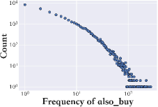
(a) Also_buy in Amazon-Book

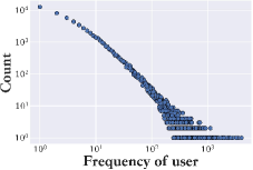
(b) Friends relationship in Yelp2022

Figure 1. Distributions of also_buy graph in Amazon-Book and friends graph in Yelp2022. To obtain the two graphs, we only keep also_buy relationship in Amazon-Book, and friends relationship in Yelp2022. The X-axis presents the frequency of nodes in sub-graphs, and the Y-axis shows the number of nodes with such frequency.

However, these works suffer from two shortcomings. First, the designs of these models only partially utilize the nature of hyperbolic space. This is mainly reflected in the following two points: 1) the initialization of the node representation treats all nodes equally, which contradicts the hierarchical structure of hyperbolic space; and 2) the information propagation of the graph convolution layer in the hyperbolic space uses the tangent space to approximate, which leads to less accurate computational results. Second, most works (He et al., 2020; Sun et al., 2021; Yang et al., 2022b, a) only focus on user-item interaction data and do not consider more side information. Although there are some works (Hu et al., 2018a; Li et al., 2020; Shi et al., 2020) integrate side information into user-item bipartite graph to construct a heterogeneous graph, they still failed to capture intrinsic characteristic in each sub-graph. Inspired by the power-law nature of user-item, we divide the heterogeneous collaborative graph into multiple side-information graphs by edge type and analyze the power-law nature of each side-information graphs. We take Amazon-Book and Yelp2022 datasets as representatives. As shown in Figure 1, we find that the sub-graph of also_buy relationship between items from Amazon-Book and the sub-graph of friends relationship between users from Yelp2022 both exhibit different power-law distributions, so they are likely to be suitable for modeling and introducing through different hyperbolic spaces to enhance the embedding of users and items to obtain better recommendation performance.

To address these challenges, we develop a novel hyperbolic GCN model for CF that incorporates multiple side information. We call our model Enhancing Hyperbolic Graph Convolution Networks on Heterogeneous Collaborative Graph (HGCC), which trains node representations by separately aggregating information in each hyperbolic subspace and fusing them in a global tengent space to obtain the final embedding. It has three novel designs: 1) power law prior-based initialization, which fully utilize heterogeneous structure of hyperbolic space and thus easier to get better training results; 2) hyperbolic information propagation, which can receive more accurate computational results than tangent space information propagation; and 3) gate fusion with prior, which better fuse different side information through training based on prior. In addition, it is worth noting that our model has only a small number of parameters added compared to the latest baseline, which further illustrates the effectiveness of our method. Overall, this work has the following contributions:

• We observe that not only user-item interaction information but also its side information has a power law nature, which indicates the implied hierarchical structure. Inspired by this, we propose a hyperbolic GCN structure for CF with fused side information.

• We propose a new method HGCC, which is equipped with power law prior-based initialization, hyperbolic information propagation, and gate fusion with prior to get better node representation.

• We conduct extensive experiments on four real datasets based on the RecBole (Zhao et al., 2021) framework to demonstrate the superior performance of the proposed method.

2. RELATED WORK

In this section, we review related work from the GCN to hyperbolic graph convolution.

2.1. Graph Convolution Neural Networks

GCN-based methods have received much attention due to their ability to learn node representations from arbitrary graph structures (Niepert et al., 2016; Welling and Kipf, 2016). They are widely used in the fields of computer vision (Liu et al., 2019b; Xu et al., 2017; Yang et al., 2018), natural language processing (Bastings et al., 2017; Welling and Kipf, 2016; Marcheggiani and Titov, 2017), and biocomputing (Duvenaud et al., 2015; Fout et al., 2017; Kearnes et al., 2016). There are also some representative GCN approaches in the field of recommender systems. NGCF (Wang et al., 2019b) generalizes GCN to the domain of recommender systems. While LightGCN (He et al., 2020) further exposes that feature transformations and nonlinear activations in GCN do not play a role in recommendation tasks and thus can be removed. DGCF (Wang et al., 2020), on the other hand, attempts to model the user’s intent using GCN. However, these approaches are mainly built in Euclidean space, which may underestimate the distribution of the user-item dataset. Recent work (Liu et al., 2019a; Chami et al., 2019; Zhang et al., 2021c) has demonstrated the potent power of hyperbolic space to model graph-structured data with hierarchical and power-law distributions.

2.2. Hyperbolic Graph Convolution Neural Networks

Recently, hyperbolic graph convolution has received increasing attention. HGNN (Chami et al., 2019), HGCN (Chami et al., 2019), and HGAT (Zhang et al., 2021b) generalize the traditional Euclidean GCN to hyperbolic spaces. LGCN (Zhang et al., 2021c) reconstructs the graph operations of a hyperbolic GCN with a Lorentzian version and designs an elegant neighborhood aggregation method based on the center of mass of the Lorentzian distance, which strictly guarantees that the learned node features follow a hyperbolic geometry. Subsequently, HYBONET (Chen et al., 2021) proposes a full hyperbolic framework that formalizes the basic operations of neural networks by adjusting Lorentz transformations (including boosting and rotation) to construct hyperbolic networks based on Lorentz models. In addition, works (Gu et al., 2018; Zhu et al., 2020) propose to use mixture curvatures to learn node representations.

2.3. Hyperbolic Recommender Systems

Hyperbolic recommender systems have been receiving more and more attention lately. HyperML (Vinh Tran et al., 2020) bridges the gap between Euclidean and hyperbolic geometry in recommender systems for the representation of the user and the item through metric learning methods. HAE and HVAE (Mirvakhabova et al., 2020) generalize AE and VAE to hyperbolic space for implicit recommendation, respectively. LKGR (Chen et al., 2022) proposes a knowledge-aware attention mechanism for hyperbolic recommender systems. In comparison, HGCF (Sun et al., 2021) implements multiple layers of skip-connected graph convolutions through tangent spaces to capture high-order connectivity information between nodes. Based on HGCF, HRCF (Yang et al., 2022b) designs a geometry-aware hyperbolic regularizer to facilitate the optimization process. Furthermore, HICF (Yang et al., 2022a) proposes an adaptive hyperbolic margin ranking loss. However, the designs of these HGCN-Based methods do not take full advantage of the nature of hyperbolic space, i.e., simplistic embedding initialization approach and message propagation by tangent space.

HSCML (Zhang et al., 2021a) provides an in-depth study of embedding techniques for recommender systems and proposes hyperbolic social collaboration metric learning by driving socially relevant users closer to each other. HME (Feng et al., 2020) applies hyperbolic space to the point-of-interest recommendation and introduces various side information such as sequential transition, user preference, category, and region information. HyperSoRc (Wang et al., 2021b) learns the representation of users and items in hyperbolic space by introducing social information. Based on HGCF, LGCF (Wang et al., 2021a) uses the midpoint of hyperbolic space to realize information propagation instead of tangent space. However, these approaches fail to simultaneously exploit the broader side information and the high-order connectivity of nodes.

3. PRELIMINARIES

In this section, we first introduce the hyperbolic space approach relevant to this paper and then present our task description.

3.1. Hyperbolic Space

We want to train low-dimensional embedding through hyperbolic space. There are many equivalent mathematical methods available, but to use the mean operation directly in hyperbolic space, we choose the Poincaré method, which has a natural generalized version of the mean (Ungar, 2008). We know that $d$-dimensional hyperbolic spaces are Riemannian manifold spaces with negative curvature, and we denote that curvature by $c$. Then denote the negative reciprocal of the curvature by $k=-1/c$ such that $k$ is non-negative. The tangent space $\mathcal{T}_{\mathbf{x}}\mathcal{M}$ of a point $\mathbf{x}$ on a manifold $\mathcal{M}$ is a $d$-dimensional Euclidean space that makes the best approximation around the point $\mathbf{x}$ on the manifold $\mathcal{M}$. The vector in $\mathcal{T}_{\mathbf{x}}\mathcal{M}$ is called the tangent vector. The representations of hyperbolic spaces are all mathematically equivalent, where the Poincaré method is defined by:

(1) $$\mathcal{B}^{d}:=\{\mathbf{x}\in\mathbb{R}^{d}:\|\mathbf{x}\|^{2}<k\},$$

where $\|\cdot\|$ denotes the Euclidean norm. The distance formula in Poincaré is:

(2) $$d_{\mathcal{B}}(\mathbf{x},\mathbf{y})=\sqrt{k}\operatorname{arcosh}\left(1+2k\frac{\|\mathbf{x}-\mathbf{y}\|^{2}}{\left(k-\|\mathbf{x}\|^{2}\right)\left(k-\|\mathbf{y}\|^{2}\right)}\right).$$

In order to extend the mathematical operation of Euclidean space to hyperbolic space, an approximation can be made with the help of tangent space $\mathcal{T}_{\mathbf{x}}\mathcal{M}$. The mapping between the tangent space and hyperbolic space is done by the exponential mapping $\text{exp}^{k}_{\mathbf{x}}$ and the logarithmic mapping $\text{log}^{k}_{\mathbf{x}}$. We fix the origin $\mathbf{o}=(0,0,\cdots,0)\in\mathcal{B}^{d}$ and use it as a reference point. In the Poincaré method, the exponential mapping $\text{exp}^{k}_{\mathbf{o}}$: $\mathcal{T}_{\mathbf{o}}\mathcal{B}^{d}\rightarrow\mathcal{B}^{d}$ is defined as (Ungar, 2008):

(3) $$\exp_{\mathbf{o}}^{k}(\mathbf{v})=\tanh(\frac{\|\mathbf{v}\|}{\sqrt{k}})\frac{\sqrt{k}\mathbf{v}}{\|\mathbf{v}\|},$$

and the logarithmic mapping $\text{log}^{k}_{\mathbf{o}}$: $\mathcal{B}^{d}\rightarrow\mathcal{T}_{\mathbf{o}}\mathcal{B}^{d}$ is given by (Ungar, 2008):

(4) $$\log_{\mathbf{o}}^{k}(\mathbf{y})=\operatorname{arctanh}(\frac{\|\mathbf{y}\|}{\sqrt{k}})\frac{\sqrt{k}\mathbf{y}}{\|\mathbf{y}\|}.$$

3.2. Task Formulation

We first introduce the concept of Heterogeneous Collaborative Graph (HCG), high-order connectivity between nodes, and compositional relations.

3.2.1. User-Item Bipartite Graphs

In a recommendation scenario, we usually have historical interaction data between users and items (e.g., purchases and visits). Here we model the interaction data as a user-item bipartite graph $\mathcal{G}_{0}=(\{\mathcal{U},\mathcal{V}\},\mathcal{E}_{0})$, where $\mathcal{U}$ and $\mathcal{V}$ represent the user set and item set, and a link $y_{u,v}=1$ in link set $\mathcal{E}$ means the user $u$ has interacted with the item $v$; otherwise $y_{u,v}=0$.

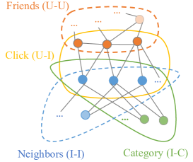
Figure 2. An Example of a Heterogeneous Collaborative Graph. Its node set contains the user, item, and category; its edge set contains the user-item link, user-user link, item-item link and item-category link.

3.2.2. Heterogeneous Collaborative Graph

We define a heterogeneous collaborative graph as $\mathcal{G}=\{\mathcal{G}_{0},\mathcal{G}_{s}\}=({\mathcal{H},\mathcal{E}})$, where $\mathcal{H}$ is node set contains user nodes $\mathcal{U}$ , item nodes $\mathcal{V}$ and other optional nodes like category nodes etc. $\mathcal{E}$ is edge set contains user-item links $\mathcal{E}_{0}$ and other kinds of links, and $\mathcal{G}_{s}=\{\mathcal{G}_{1},\mathcal{G}_{2}\cdots\mathcal{G}_{|\mathcal{S}|-1}\}$ denotes the set of all side-information graphs. Heterogeneous collaborative graph $\mathcal{G}$ is also associated with a node type mapping function $\phi:\mathcal{H}\rightarrow\mathcal{T}$ and a link type mapping function $\psi:\mathcal{E}\rightarrow\mathcal{S}$. $\mathcal{T}$ and $\mathcal{S}$ denote predefined node types and link types, where $|\mathcal{T}|+|\mathcal{S}|>2$. Figure 2 is an example of the HCG.

3.2.3. Task Description

We then formalize the recommendation task to be solved in this paper:

• Input: heterogeneous collaborative graph $\mathcal{G}$ that includes user-item interaction graph $\mathcal{G}_{0}$ and side information subgraph $\mathcal{G}_{s}$.

• Output: a function that gives the probability $\hat{y}_{u,v}$ that user $u$ accepts item $v$.

4. METHOD

We now propose the HGCC model. Its framework is shown in Figure 3 with three main components: 1) power law prior-based embedding layer initializes each node as a vector in tangent space based on popularity; 2) hyperbolic propagation and fusion layer performs recursive operations, projects into hyperbolic subspaces for neighbor information aggregation, then back to tangent space for embedding update through gate fusion with prior; and 3) prediction layer aggregates node representations and projects into hyperbolic space to produce matching scores.

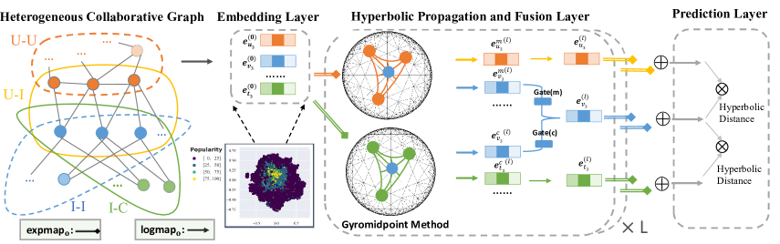
Figure 3. The overall framework of the proposed HGCC. It consists of three main components: 1) power law prior-based embedding layer, 2) hyperbolic propagation and fusion layer, and 3) prediction layer.

4.1. Embedding Layer with Power Law Prior

Current hyperbolic recommender systems have two approaches for embedding training: 1) defining it in hyperbolic space and initializing it by sampling in tangent space then mapping it back to hyperbolic space, and training with a Riemann optimizer (Feng et al., 2020; Sun et al., 2021; Yang et al., 2022a, b); 2) defining and initializing in tangent space (Euclidean space) and training with a Euclidean optimizer (Xu et al., 2022). We communicated with the author of AMCAD (Xu et al., 2022) and found that defining node embeddings in hyperbolic space does not bring significant benefits. Our earlier experiments also led to the same conclusion. Thus, we define and initialize node embeddings in tangent space.

The initialization of embedding parameters can impact optimization results (Glorot and Bengio, 2010). Proper initialization leads to better results, while poor initialization may cause difficulties and reach local optimums. Previous works (Feng et al., 2020; Sun et al., 2021; Yang et al., 2022a, b) initialized node embeddings by sampling from uniform or Gaussian distributions in tangent space. However, existing research (Feng et al., 2020; Sun et al., 2021) shows that the norm magnitude of the hyperbolic space embedding is related to node popularity, with more popular nodes closer to the origin and less popular nodes further away. A uniform or Gaussian prior distribution for all nodes may result in incorrect initialization of popular nodes away from the origin, potentially causing the model to reach a local optimum during training.

Toward this end, we propose power law prior-based initialization, which allows each node to use different parameter initialization according to its popularity, making it easier for nodes with higher popularity to be initialized closer to the origin. Formally, based on a given uniform distribution, the power law prior-based sampling distribution of node $n$ is:

(5) $$\mathbf{e}^{(0)}_{n}\sim\text{Uni}(-ax_{n}^{-b},ax_{n}^{-b}),\\$$

where $x_{n}$ denotes the frequency of node $n$, $a$ is the scale of initialization consistent with uniform initialization, and $b$ is the hyperparameter of power law distribution which is set to 1.1 empirically. It is important to note that since $\text{exp}^{k}_{\mathbf{o}}$ and $\text{log}^{k}_{\mathbf{o}}$ are both conformal (Ungar, 2008), the prior is still kept in mapped embeddings.

4.2. Hyperbolic Propagation and Fusion Layers

Next, we establish the structure of the hyperbolic graph convolution layer to recursively propagate embedding and fuse information from different subspaces through high-order connectivity. Here, we start by describing a single layer consisting of two components: hyperbolic information propagation and gate fusion with prior. Then we discuss how to generalize to multiple layers.

4.2.1. Hyperbolic Information Propagation

Previous work (Chami et al., 2019) extend the Euclidean GCN information propagation to hyperbolic space by the tangent space method. Specifically, the hyperbolic space embedding is first projected to the tangent space at the origin by the $\text{log}^{k}_{\mathbf{o}}$, then the Euclidean GCN information propagation is applied, and finally, the embedding is projected back to the hyperbolic space by the $\text{exp}^{k}_{\mathbf{o}}$. Through this way, the GCN information propagation in hyperbolic space can be approximated. Formally, given a hyperbolic space embedding of node $n$, its tangent space message propagation proceeds according to the following equations:

(6) $$\mathbf{e}^{(l-1)}_{n} = \log_{\mathbf{o}}^{k}(\mathbf{h}^{(l-1)}_{n}),$$

(7) $$\mathbf{e}^{(l)}_{n} = \sum\limits_{i\in\mathcal{N}_{n}}\frac{1}{|\mathcal{N}_{n}|}\mathbf{e}^{(l-1)}_{i},$$

(8) $$\mathbf{h}^{(l)}_{n} = \exp_{\mathbf{o}}^{k}(\mathbf{e}^{(l)}_{n}),$$

where $\mathcal{N}_{n}$ denotes the set containing node $n$ itself and its neighbors. However, this approach hinders the performance for two reasons: 1) the operation in tangent space is an approximation of the hyperbolic space operation, which introduces errors; and 2) the information propagation of all nodes is performed in the tangent space of the origin instead of its own tangent space, which further introduces errors. We want to reduce the error of hyperbolic information propagation for better performance, which requires direct implementation of information propagation in hyperbolic space. For this purpose, we use the gyromidpoint method (Ungar, 2008):

(9) $$m\left(\mathbf{x}_{1},\ldots,\mathbf{x}_{N};\bm{\nu}\right)=\frac{1}{2}\oplus_{k}\left(\sum_{i=1}^{N}\frac{\nu_{i}\lambda(k,{\mathbf{x}_{i}})}{\sum_{j=1}^{N}\nu_{j}\left(\lambda(k,{\mathbf{x}_{j}})-1\right)}\mathbf{x}_{i}\right),$$

where $\nu_{i}$ is the weight of node $\mathbf{x}_{i}$, $\lambda(k,{\mathbf{x}})=2\left(1-\frac{\|\mathbf{x}\|^{2}}{k}\right)^{-1}$, and $\oplus$ is the Möbius addition (Ungar, 2008). For $\nu_{i}$, we set it to 1, i.e., all nodes contribute equally. Other methods, such as the attention mechanism (Bahdanau et al., 2014), can learn the different importance of different nodes, but this is not the focus of this paper, so we leave it for future work.

Hence, given the tangent space embedding of a node $n$ of $(l-1)$-th layer, we want to get the neighbor information of $n$ from subgraph $\mathcal{G}_{s}$. We first project it into the hyperbolic subspace $s$ by $\text{exp}^{k}_{\mathbf{o}}$:

(10) $$\mathbf{h}^{s,(l-1)}_{n}=\exp_{\mathbf{o}}^{k_{s}}(\mathbf{e}^{(l-1)}_{n}),$$

and then perform information propagation by Equation 9:

(11) $$\mathbf{h}^{s,(l)}_{n}=\frac{1}{2}\oplus_{k_{s}}\left(\sum_{i\in\mathcal{N}_{n}}\frac{\lambda({k_{s}},{\mathbf{h}^{s,(l-1)}_{i}})}{\sum_{j\in\mathcal{N}_{n}}\left(\lambda({k_{s}},{\mathbf{h}^{s,(l-1)}_{j}})-1\right)}\mathbf{h}^{s,(l-1)}_{n}\right),$$

thus aggregating information from neighboring nodes directly in hyperbolic space. We further analyze why the midpoint method works in Section 5.2.

4.2.2. Multi-Space Information Fusion

After information propagation in each subspace, we need to fuse the output from each subspace to update the embedding of the nodes. Since the curvature of each subspace is not necessarily the same, we need to project the embedding to a uniform tangent space first, as follows:

(12) $$\mathbf{e}^{s,(l)}_{n}=\log_{\mathbf{o}}^{k_{s}}(\mathbf{h}_{n}^{s,(l)}).$$

Then we can consider the fusion of multiple information in the tangent space, which is:

(13) $$\mathbf{e}^{(l)}_{n}=\sum_{s\in\mathcal{S}_{n}}\mathbf{g}_{n}^{s}\odot\mathbf{e}^{s,(l)}_{n},$$

where $\mathcal{S}_{n}$ is the set of subspaces that node $n$ involves in, $\odot$ is element-wise product and $\mathbf{g}_{n}^{s}$ is the weight of embedding $\mathbf{e}_{n}^{s}$. An intuitive idea is to set a learnable weight to control the weight of each kind of information automatically. Accordingly, we use the gate mechanism to implement this idea, which we call gate fusion. It is formulated as follows:

(14) $$\mathbf{g}_{\text{gate}}=\frac{\sigma(\mathbf{W}_{t_{n}}^{s}\mathbf{e}_{n}^{(0)})}{\sum_{i\in\mathcal{S}_{n}}\sigma(\mathbf{W}_{t_{n}}^{i}\mathbf{e}_{n}^{(0)})},$$

where $t_{n}$ is the type of node $n$, i.e., $t_{n}\in\{\textit{user},\textit{item},\textit{category},\cdots\}$, $\mathbf{W}^{s}_{t_{n}}$ is the learnable parameter of the gate of subspace $s$ corresponding to the type of node $n$, and $\sigma$ is the sigmoid function. However, in practice, we found that gate fusion can easily fall into the local optimum and even perform less well than the model without side information in some cases. So we directly use normalized neighbor numbers of node $n$ in subspace $s$ as a prior weight, namely prior-based fusion, and it is given by:

(15) $$\mathbf{g}_{\text{prior}}=\frac{|{\mathcal{N}_{n}^{s}}|}{\sum_{i\in{\mathcal{S}_{n}}}|{\mathcal{N}_{n}^{i}}|}.$$

What is more, if the gate fusion can learn based on prior instead of learning from scratch, the performance may get further improvement. Therefore, we combine the two and call this approach the gate fusion with prior, which is defined as:

(16) $$\mathbf{g}_{\text{gate\&prior}}=\frac{|{\mathcal{N}_{n}^{s}}|\sigma(\mathbf{W}_{t_{n}}^{s}\mathbf{e}_{n}^{(0)})}{\sum_{i\in\mathcal{S}_{n}}|{\mathcal{N}_{i}^{s}}|\sigma(\mathbf{W}_{t_{n}}^{i}\mathbf{e}_{n}^{(0)})}.$$

According to experiments, gate fusion with prior is better in most cases, so we adopt this structure for HGCC. The empirical comparison of these structures is shown in Section 6.5.

Although we avoid the computational error of information propagation, we still inevitably bring computational error when introducing side information. However, it is confirmed by Section 6.5 that the benefits of introducing side information far outweigh the drawbacks. Besides, we also use the learnable gate method as a remedy for the computational error. If both information propagation and information fusion are implemented in tangent space, two computational errors will be accumulated.

4.2.3. High-Ordrer Propagation

Further, we can stack multiple layers to explore high-order connectivity information and collect multiple information from multi-hop neighbors. More specifically, in step $l$, we recursively formulate the representation of node $n$ as:

(17) $$\mathbf{e}_{n}^{(l)}=f\left(\mathbf{e}_{n}^{(0)},\mathbf{e}_{\mathcal{N}_{n}}^{(l-1)}\right).$$

However, previous work (Sun et al., 2021) found that stacking multiple layers leads to degradation in the model’s overall performance due to gradient disappearance and over smoothing. Here, we refer to HGCF (Sun et al., 2021) and use SkipGCN to aggregate the output of multiple layers, which is defined as follows:

(18) $$\mathbf{e}_{n}=\sum_{i=1}^{L}\mathbf{e}_{n}^{(i)},$$

where $L$ is the number of convolutional layers. In this way, the final output of the convolutional layer embedding contains rich neighbor information and side information, and we next employ the hyperbolic distance $d_{\mathcal{B}}$ to evaluate the similarity of node pairs.

4.3. Prediction Layer

The embeddings of the final output are first projected into the hyperbolic space of the scoring layer, and then the formula $d_{\mathcal{B}}$ in Equation 2 is used to evaluate the similarity of the node pairs $(i,j)$, more formally, as defined below:

(19) $$\mathbf{h}_{i} = \exp_{\mathbf{o}}^{k_{s}}(\mathbf{e}_{i}),$$

(20) $$\mathbf{h}_{j} = \exp_{\mathbf{o}}^{k_{s}}(\mathbf{e}_{j}),$$

(21) $$\hat{y}_{i,j} = -d_{\mathcal{B}}(\mathbf{h}_{i},\mathbf{h}_{j})^{2}.$$

Thus the prediction of the node pair ratings is completed.

4.4. Optimization

In our experience, the margin ranking loss used by HGCF (Sun et al., 2021) is essential to optimize our model and is given as belows:

(22) $$\mathcal{L}_{\text{CF}}=\mathcal{L}_{\mathcal{G}_{0}}=\max\left(\hat{y}_{u,j}-\hat{y}_{u,i}+m,0\right),$$

where $m$ is margin, item $i$ is a positive sample sampled from $y_{u,i}=1\in\mathcal{G}_{0}$, and item $j$ is a negative item sampled from $\mathcal{V}$. The margin $m$ means the minimum difference required between positive and negative sample scores. As $m$ approaches infinity, the margin ranking loss becomes equivalent to the BPR Loss (Rendle et al., 2009). However, this causes the model to focus too much on simple pairs, making training slow and reducing performance by causing many embeddings to gather near the boundaries of the ball. For other subgraphs $\mathcal{G}_{s}$, we also train their embeddings by margin ranking loss:

(23) $$\mathcal{L}_{\text{SI}}=\sum_{\mathcal{G}_{i}\in\mathcal{G}_{s}}\mathcal{L}_{\mathcal{G}_{i}},$$

where node $\mathcal{G}_{i}$ denotes subgraphs of each link type, and we only sample negative nodes in subgraph $\mathcal{G}_{i}$ when calculating $\mathcal{L}_{\mathcal{G}_{i}}$. Eventually, our total objective function takes the multitask form with $\mathcal{L}_{\text{CF}}$ as the target task and $\mathcal{L}_{\text{SI}}$ as the auxiliary task:

(24) $$\mathcal{L}=\mathcal{L}_{\text{CF}}+\alpha\mathcal{L}_{\text{SI}},$$

where $\alpha$ is the hyperparameter controlling the weight of the auxiliary task $\mathcal{L}_{\text{SI}}$ being set to 0.01 empirically.

4.5. Training

Unlike previous approaches that employ Riemann optimizers such as RSGD (Bonnabel, 2013; Nickel and Kiela, 2018; Wilson and Leimeister, 2018) and RAdam (Becigneul and Ganea, 2018) to optimize hyperbolic embedding, all of our trainable parameters are defined in Euclidean space, so we can directly use optimization techniques that are well established in Euclidean space.

5. DISCUSSION

5.1. Space Complexity Analysis

The space complexity of HGCC is mainly composed of two parts: 1) node embedding, which is $\mathcal{O}(|\mathcal{H}|d)$; and 2) gate, which is $\mathcal{O}(|\mathcal{G}|d^{2})$. Hence the total space complexity is $\mathcal{O}((|\mathcal{H}|+|\mathcal{G}|d)d)$. When the data used is only user-item interaction data, the space complexity of HGCC is $\mathcal{O}(|\mathcal{H}|d)$, which is consistent with the lightweight models having only embedding parameters such as LightGCN (He et al., 2020) and HGCF (Sun et al., 2021); when the data used contains side information, the numbers of new node from side graph are generally not significant in real scenarios. Besides, it is often $|\mathcal{H}|\gg|\mathcal{G}|d$, so HGCC only adds a small number of parameters in this case.

5.2. Anaysis of Gyromidpoint

Here, we try to analyze more specifically how the information propagation through gyromidpoint differs from the way by tangent space, to explain why hyperbolic information propagation may be more effective. Substituting Equation 10 into $\lambda({k},{\mathbf{h}_{i}})$ and omit the notation of subspace and the number of layer for simplicity, we get:

(25) $$\lambda(k,{\mathbf{h}_{i}}) = 2\left(1-\frac{\|\mathbf{h}_{i}\|^{2}}{k}\right)^{-1}$$

$$= 2(1-\text{tanh}^{2}(\frac{\|\mathbf{e}_{i}\|}{\sqrt{k}}))^{-1}.$$

We notice that when fixing the negative reciprocal of the curvature $k$, the magnitude of $\lambda(k,{\mathbf{h}_{i}})$ positively correlates with the magnitude of $\mathbf{e}_{i}$. Furthermore, the role of $\lambda(k,{\mathbf{h}_{i}})$ in equation 9 is similar to the weight of node $\mathbf{h}_{i}$, which means that the node with a larger embedding magnitude in tangent space has a more significant weight in information propagation. Therefore, combining the relationship between embedding magnitude and popularity in hyperbolic space, we can find that: in gyromidpoint information propagation, nodes with lower popularity are more likely to contribute more. While tangent space information propagation only directly averages all the nodes being aggregated, and its corresponding Laplace matrix is $\mathbf{D}^{-1}\mathbf{A}$ ($\mathbf{A}$ is the adjacency matrix, and $\mathbf{D}$ is the degree matrix), which does not explicitly weaken the contribution of high popularity nodes, thus may lead to the degradation of performance. There is also a commonly used Laplacian matrix of $\mathbf{D}^{-\frac{1}{2}}\mathbf{A}\mathbf{D}^{-\frac{1}{2}}$, which does a second averaging according to the popularity of the nodes being aggregated, but in practice, it yields a worse performance under the hyperbolic space scenario.

5.3. Relation to Heterogeneous Graph Methods

Heterogeneous graph recommendations almost always use path-based methods. Path-based methods extract the information from high-order paths and feed it into the model. To handle numerous relationships between nodes, it either uses a path selection algorithm to choose the salient paths (Sun et al., 2018; Wang et al., 2019c) or a predefined meta-path approach (Hu et al., 2018b; Yu et al., 2013; Sun et al., 2011; Jin et al., 2020). The goodness of the paths has a significant impact on the final performance, but these paths cannot be optimized with the recommended goals, or the definition of effective meta-paths requires significant domain knowledge and is likely not optimal. Traditional heterogeneous graph methods are unsolvable in the face of vast and complex nodes and relations (Wang et al., 2019a). In contrast, our approach processes and fuses different node relationships separately by hyperbolic subspace and multi-space information fusion and then further realizes the path combination of multiple relationships by the high-order connectivity brought by multi-layer GCN.

6. EXPERIMENTS

We evaluate our proposed approach on four real data sets. We want to answer the following research questions:

• RQ1: How does HGCC perform compared to the state-of-the-art recommender methods?

• RQ2: What is the impact of each component (i.e., power law prior-based initialization, hyperbolic information propagation, and gate fusion with prior) on HGCC?

• RQ3: How well do different fusion methods work on HGCC?

• RQ4: What kind of embedding has HGCC method learned?

6.1. Dataset Description

We evaluate the proposed method on four public available benchmark: Amazon-CD, Amazon-Book¹, Gowalla, and Yelp2022. They differ in domain, size, sparsity, and side information. To introduce side information, we had to process the raw data from scratch as previous works (Wang et al., 2019b; He et al., 2020) only provided processed interaction datasets without a script for processing data. Referring to previous work (Wang et al., 2019b; He et al., 2020) for ensuring fairness, we use a 10-core setting for Amazon-Book, Gowalla, and Yelp2022, but a 10-core setting and 5-core setting for the user and item of Amazon-CD, respectively, because of its small size. Besides, we transform the ratings into binary preferences with a threshold $\geq$ 4 to simulate implicit feedback.

Table 1. Interaction information statistics for datasets.

Dataset	#User	#Item	#Interaction	Density
Amazon-CD	16865	33900	476676	0.083%
Amazon-Book	109730	96421	3181759	0.030%
Gowalla	29858	40988	1027464	0.084%
Yelp2022	93537	53347	2533759	0.051%

Table 2. Side information statistics for datasets. U, I, and C represent user, item, and category respectively.

Dataset	Relation(A-B)	#A	#B	#A-B
Amazon-CD	category(C-I)	380	33900	68382
	also_view(I-I)	33900	33900	121149
Amazon-Book	also_buy(I-I)	96421	96421	347311
	also_view(I-I)	96421	96421	159154
Gowalla	friend(U-U)	29858	29858	279478
	neighbor(I-I)	40988	40988	501242
Yelp2022	friend(U-U)	93537	93537	1295854
	neighbor(I-I)	53347	53347	1038744

Moreover, we need to build side information bipartite graphs (referred to as side graphs for short) for each dataset. For Amazon-CD and Amazon-Book, we choose $\{$category(C-C), also$\_$view(I-I)$\}$ and $\{$also$\_$buy(I-I), also$\_$view(I-I)$\}$ respectively to build the side graph. For the side graph of Gowalla and Yelp2022, we first choose social information (U-U) and then construct geographic neighborhood information (I-I) from latitude and longitude, which is an important feature in poi recommendation. We approximate the earth as a sphere with a radius of 6371 km and use the haversine function to calculate the geographical distance $d_{geo}$ between two locations. Locations within a geographical distance of 0.2 km are considered neighbors and form the geographical neighbor graph.

We present the statistics of historical interaction data and side information for the four datasets in Table 1 and Table 2. For each dataset, we divide it into a training set and a test set with a ratio of 8:2. Then, 10$\%$ of the training set is randomly selected as the validation set for tuning hyperparameters.

6.2. Experimental Settings

6.2.1. Evaluation Metrics

We adopt two widely-used evaluation protocols (Järvelin and Kekäläinen, 2002) recall@$K$ and ndcg@$K$ as evaluation metrics on the test set, where $K$ is taken as 10 and 20.

Table 3. Performances for all datasets. The best performing model on each dataset and metric is highlighted in bold, and second best model is underlined. Asterisks denote statistically significant Wilcoxon signed rank test for the difference in scores between the best and second-best models. Some results are inconsistent with the original paper because we used the model replicated by the open-source platform and reprocessing dataset from scratch due to the introduction of side information.

Datasets	Metric	BPRMF	WRMF	NGCF	LightGCN	DGCF	HGCF	HRCF	HGCC	HGCF+	HRCF+	HGCC+	%Imporv.
Amazon-CD	R@10	0.0666	0.0762	0.0710	0.0834	0.0765	0.0975	0.0997	0.1000*	0.1055	0.1029	0.1100*	10.33%
	R@20	0.1036	0.1147	0.1092	0.1259	0.1138	0.1436	0.1457	0.1478*	0.1585	0.1543	0.1631*	11.94%
	N@10	0.0553	0.0631	0.0586	0.0688	0.0633	0.0823	0.0831	0.0844*	0.0872	0.0847	0.0915*	10.11%
	N@20	0.0672	0.0756	0.0710	0.0825	0.0754	0.0969	0.0976	0.0994*	0.1042	0.1012	0.1084*	11.07%
Amazon-Book	R@10	0.0666	0.0609	0.0637	0.0827	0.0714	0.0983	0.0979	0.1048*	0.1008	0.1008	0.1104*	12.31%
	R@20	0.0998	0.0927	0.0974	0.1215	0.1069	0.1413	0.1413	0.1489*	0.1451	0.1451	0.1560*	10.40%
	N@10	0.0537	0.0511	0.0523	0.0690	0.0591	0.0835	0.0830	0.0905*	0.0845	0.0843	0.0947*	13.41%
	N@20	0.0645	0.0614	0.0632	0.0815	0.0706	0.0972	0.0969	0.1044*	0.0987	0.0985	0.1091*	12.24%
Gowalla	R@10	0.1075	0.0999	0.1143	0.1286	0.1204	0.1296	0.1303	0.1379*	0.1392	0.1409	0.1502*	15.27%
	R@20	0.1578	0.1499	0.1697	0.1853	0.1755	0.1912	0.1914	0.2007*	0.2053	0.2061	0.2177*	13.74%
	N@10	0.1035	0.0926	0.1110	0.1262	0.1171	0.1237	0.1247	0.1327*	0.1343	0.1351	0.1448*	14.74%
	N@20	0.1188	0.1093	0.1277	0.1432	0.1338	0.1420	0.1428	0.1510*	0.1538	0.1546	0.1646*	14.94%
Yelp2022	R@10	0.0500	0.0629	0.0546	0.0655	0.0609	0.0667	0.0649	0.0730*	0.0607	0.0604	0.0746*	11.84%
	R@20	0.0838	0.1017	0.0897	0.1057	0.0986	0.1109	0.1095	0.1198*	0.1025	0.1013	0.1219*	9.92%
	N@10	0.0409	0.0514	0.0448	0.0552	0.0508	0.0549	0.0536	0.0609*	0.0495	0.0491	0.0626*	13.41%
	N@20	0.0520	0.0642	0.0563	0.0682	0.0629	0.0693	0.0681	0.0758*	0.0631	0.0625	0.0777*	12.12%

6.2.2. Baselines

To show the effectiveness of our model, we compare our proposed HGCC with latent factor-based (BPRMF (Rendle et al., 2009) and WRMF (Hu et al., 2008)), graph neural network-based (NGCF (Wang et al., 2019b), LightGCN (He et al., 2020), and DGCF (Wang et al., 2020)), and hyperbolic neural network-based (HGCF (Sun et al., 2021) and HRCF (Yang et al., 2022b)). Besides, we refer to the version using HCG directly as HGCF+ and HRCF+, respectively.

• BPRMF (Rendle et al., 2009) is based on Bayesian personalized ranking, which models the order of candidate items by pairwise ranking loss.

• WRMF (Hu et al., 2008) is a classical latent factor model that attaches a weight to each training sample to characterize the confidence level of the user’s preference for the items.

• NGCF (Wang et al., 2019b) is a GCN-based model that explores high-order connectivity in the user-item graph by propagating embedding and injects collaboration signals into the embedding explicitly.

• LightGCN (He et al., 2020) is a state-of-the-art GCN model, which removes feature transformations and nonlinear activations that are useless for collaborative filtering in GCN.

• DGCF (Wang et al., 2020) uses GCN to encode graph structure data and iteratively refines intention-aware interaction graphs and representations by modeling the intention distribution of each user-item interaction. Here, we follow the original paper to set its graph disentangling layer to 1 because of high computational cost.

• HGCF (Sun et al., 2021) is a leading hyperbolic GCN model, which replaces the traditional Euclidean space with Lorentz space, and learns embedding by Skip-GCN structure and margin ranking loss.

• HRCF (Yang et al., 2022b) is a state-of-the-art hyperbolic GCN model, which is based on HGCF and adds a geometry-aware hyperbolic regularizer to boost optimization.

There are other hyperbolic neural network-based models, such as the recent LGCF (Wang et al., 2021a) and HICF (Yang et al., 2022a), but we do not include them in the baseline because they are not directly open source until our work was completed. For our model, we denote the version that uses only the user-item bipartite graph and the version that utilizes HCG as HGCC and HGCC+, respectively. Note that the main difference between HGCF+/HRCF+ and HGCC+ is the information propagation, the former proceeds directly on the HCG, but the latter performs on each subgraph of the HCG separately.

6.2.3. Hyperparameter Settings

We implemented our models and baselines based on the RecBole (Zhao et al., 2021) framework. All baseline settings and training strategies refer to the original authors’ implementation and further tune the parameters based on it. For fairness, the embedding size of all models is fixed to the widely used 64. We use the Adam optimizer (Kingma and Ba, 2015) to optimize all models except HGCFs/HRCFs which are RSGD because their parameters are defined in hyperbolic space. The gate parameters of HGCC+ and the parameters of other models are initialized using Xavier initializer (Glorot and Bengio, 2010) except for the embedding weight of HGCFs/HRCFs and HGCCs, which use uniform initializer and power law prior-based initializer, respectively. For NGCF, LightGCN, HGCFs, and HGCCs, we set their GCN layers to 3. We apply a grid search to the hyperparameters: the batch size of the different models on each dataset is tuned in $\{$1024, 2048, 4096, 8192$\}$ and the learning rate is tuned amongst $\{$0.01, 0.005, 0.001, 0.0005, 0.0001$\}$, weight decay or $L_{2}$ normalization is search in $\{$0.01, 0.005, $\cdots$, $5\times 10^{-5}$,$10^{-6}\}$, and the dropout ratio is tuned in $\{$0.0, 0.1, $\cdots$, 0.5$\}$ for NCF, NGCF. Besides, we employ the node dropout technique for NGCF, where the ratio is searched in $\{$0.0, 0.1, $\cdots$, 0.5$\}$. For WRMF, we select the positive item weight from $\{$1, 10, 100, 1000, 10000$\}$. For NCF, the ratio of positive and negative samples for negative sampling is 1:4, which follows the original setting. For DGCF, the iteration number and latent intents are set to 2 and 4, respectively, and the correlation weight is tuned amongst $\{$0.005,0.01,0.02,0.05$\}$. For HRCF, the $\lambda$ in the loss function is in the range of {10, 15, 20, 25, 30} and the layers of GCN is searched from 2 to 10. For our model, we set all curvatures to 1 for simplicity, leaving the exploration of different hyperbolic subspace curvatures with possible performance gains to future work. Besides, we refer to previous work (Xu et al., 2022) using dynamic negative sampling, which speeds up the convergence of models. Moreover, we discovered that certain models, including HGCFs, exhibited relatively slow convergence, and to more fairly reflect that we increase the upper limit of the model performance, all models are trained for 1000 epochs, and the early stopping strategy is applied, i.e., premature stopping if ndcg@10 on the validation set does not increase for 100 successive epochs.

Table 4. Ablation analysis on Amazon-Book and Yelp2022.

Arch.	Amazon-Book		Yelp2022
	R@20	N@20	R@20	N@20
HGCN	0.1339	0.0947	0.1113	0.0710
HGCN+HI	0.1457	0.1024	0.1180	0.0749
HGCN+PI	0.1470	0.1032	0.1197	0.0762
HGCC	0.1489	0.1044	0.1198	0.0758
HGCC+	0.1560	0.1091	0.1219	0.0777

6.3. Performance Comparison (RQ1)

The results of the performance comparison are shown in Table 3, where we have the following observations:

• HGCC consistently outperforms all baseline methods when only interaction data are available. Notably, HGCF, HRCF, and HGCC are all hyperbolic GCN models, while HGCF performs well on the Amazon dataset, but its metric ndcg is slightly weaker than LightGCN on Gowalla and Yelp2022, similar to the report of HGCF. Although HRCF is improved based on HGCF, it does not show many advantages in our experiment. It seems that the authors of HGCF believe this phenomenon is related to the density of the data (Sun et al., 2021). However, in our experiments, Amazon-CD and Gowalla densities are almost the same, Amazon-Book is even sparser than Yelp2022, and the most significant commonality between Gowalla and Yelp2022 is that they are both Check-in dataset. Therefore, we believe that it may be the design flaw of HGCF/HRCF itself that causes its poor performance on Check-in class datasets. In contrast, our proposed power law prior-based initialization and hyperbolic information propagation remedy these defects and improve further.

• After introducing side information, the performance of the hyperbolic GCN methods is further improved compared to their base versions except for HGCF+ and HRCF+ on the Yelp2022 dataset, and the latter improvement is more significant than that of the former. In particular, unlike HGCC+, HGCF+ and HRCF+ have decreased on the Yelp2022 dataset, which fully demonstrates the possible drawbacks caused by the direct use of HCG. The above mentioned phenomena demonstrate that HGCC can utilize the side information more effectively.

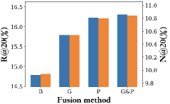
(a) Amazon-CD

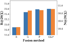
(b) Amazon-Book

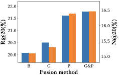
(c) Gowalla

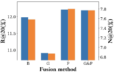
(d) Yelp2022

Figure 4. Comparison between different fusion methods. B, G, P, and G&P represent Base, Gate, Prior, and Gate&Prior, respectively, where the Base is the HGCC.

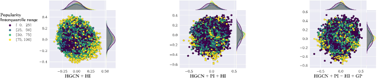
(a) Item embeddings before the graph convolution layers

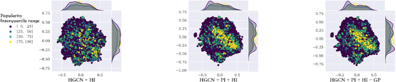
(b) Item embeddings after the graph convolution layers

Figure 5. HGCC item embedding visualization in the Poincaré representation of tangent space before and after the graph convolutional layers on the dataset Amazon-Book. HGCC is trained with three graph convolution layers and embedding dimension set to 2. Items are categorized into quartiles by popularity, where [75, 100] represents the most popular items. The meaning of HGCN, PI, HI, and GP are the same as in Section 6.4.

6.4. Ablation Analysis (RQ2)

To evaluate the contribution of each component of HGCC to the overall performance, we conducted extensive ablation experiments, and the results are shown in Table 4. HGCN is a hyperbolic GCN model with Euclidean-defined parameters and trained with uniform distribution for initialization, tangent space for information propagation, and Poincaré distance for score prediction. HGCN+HI replaces tangent space information propagation with hyperbolic propagation. Then HGCN+PI is a version of HGCN with power law prior-based initialization. Our HGCC model is HGCN+PI+HI, combining power law prior-based initialization and hyperbolic information propagation. Finally, HGCC+ (HGCN+PI+HI+GP) fuses side information through a gate fusion with prior. From the results in Table 4, we can see that:

• HGCN+HI brings significant improvement, which may be because hyperbolic information propagation can bring more accurate computational results than tangent information propagation.

• HGCN+PI also dramatically improves the performance compared to HGCN, which may be attributed to the power law prior-based initialization giving more information to the initial embedding.

• The combination of PI and HI further improves the performance on the Amazon-Book dataset, indicating that the power law prior-based initialization and hyperbolic information propagation may improve the performance of HGCN from different aspects. Nevertheless, the case is different on the Yelp2022 dataset, where the performance does not get promoted, which may attribute to the difference in nature between datasets.

• The performance is again greatly improved by adding GP, which verifies the effectiveness of GP and side information.

6.5. Comparison of Fusion Methods (RQ3)

We evaluated the impact of different fusion methods on the model performance. Figure 4 shows the results of the fusion methods introduced in Section 4.2.2, where the Base is the version without side information. We observe two phenomena:

• Except for gate in the Yelp2022 dataset, all three fusion methods bring performance improvement compared to the Base, indicating that these fusion methods basically incorporate side information into embedding.

• The improvement of the Gate is always the least, even worse than the Base in the dataset Yelp2022, which shows how difficult it is to train the gate from scratch, and it is easy to fall into local optimum. After incorporating the prior in the gate, the performance is comparable to and slightly improved by the prior method, indicating that it is possible for the gate to further learn more appropriate weights based on the prior.

6.6. Embedding Visualization Analysis (RQ4)

The rich structure of hyperbolic spaces has been used to gain meaningful insights into the underlying data structure (Nickel and Kiela, 2017b). In this section, we will provide a possible interpretation of our proposed approach by visualizing the embedding learned by HGCC. Since our model is based on the Poincaré disc, it can be easily visualized. We use a 3-layer HGCC model with its embedding size set to 2 for visualization, which follows previous work (Feng et al., 2020; Sun et al., 2021). To understand the learned embeddings, we take the Amazon-Book dataset as a representative, color the embeddings with quartiles of the number of interactions as node labels, and show the embeddings before and after graph convolution.

Figure 5 shows the distribution of the embedding learned by the model on the Amazon-Book dataset with uniform initialization as the base and after adding the power law prior-based initialization and side information sequentially. Before the graph convolution, items show Gaussian-like distribution in both dimensions, and the nodes with higher popularity are more concentrated at the origin after adding the power law prior-based initialization and side information, which suggests that power law prior-based initialization may be helpful for embedding training. Besides, after graph convolution, the class boundaries of the power law prior-based initialization are more evident than the uniform initialization. Moreover, in terms of node distribution, nodes with higher popularity are closer to the origin after adding side information, which seems to indicate that side information also improves performance by promoting node distribution according to popularity.

7. CONCLUSION AND FUTURE WORK

This paper presents a hyperbolic GCN collaborative filtering model, HGCC, which fuses side information. Each user and item is defined in Euclidean space and initialized by popularity, and then information is mined and fused through hyperbolic information propagation and multi-space information fusion. The model further stacks multiple layers to capture node high-order connectivity. Experiments on four real-world datasets show significant improvements over baselines, with meaningful structures in the learned representations. In the future, we intend to explore the popularity bias in hyperbolic space to investigate whether it improves performance by reducing the bias.

References

- (1)
- Adcock et al. (2013) Aaron B. Adcock, Blair D. Sullivan, and Michael W. Mahoney. 2013. Tree-Like Structure in Large Social and Information Networks. In 2013 IEEE 13th International Conference on Data Mining. 1–10.
- Bahdanau et al. (2014) Dzmitry Bahdanau, Kyunghyun Cho, and Yoshua Bengio. 2014. Neural machine translation by jointly learning to align and translate. arXiv preprint arXiv:1409.0473 (2014).
- Bastings et al. (2017) Jasmijn Bastings, Ivan Titov, Wilker Aziz, Diego Marcheggiani, and Khalil Sima’an. 2017. Graph Convolutional Encoders for Syntax-aware Neural Machine Translation. In Proceedings of the 2017 Conference on Empirical Methods in Natural Language Processing. Association for Computational Linguistics, Copenhagen, Denmark, 1957–1967.
- Becigneul and Ganea (2018) Gary Becigneul and Octavian-Eugen Ganea. 2018. Riemannian Adaptive Optimization Methods. In International Conference on Learning Representations.
- Bonnabel (2013) Silvere Bonnabel. 2013. Stochastic gradient descent on Riemannian manifolds. IEEE Trans. Automat. Control 58, 9 (2013), 2217–2229.
- Chami et al. (2019) Ines Chami, Zhitao Ying, Christopher Ré, and Jure Leskovec. 2019. Hyperbolic Graph Convolutional Neural Networks. In Advances in Neural Information Processing Systems, H. Wallach, H. Larochelle, A. Beygelzimer, F. d'Alché-Buc, E. Fox, and R. Garnett (Eds.), Vol. 32. Curran Associates, Inc.
- Chen et al. (2021) Weize Chen, Xu Han, Yankai Lin, Hexu Zhao, Zhiyuan Liu, Peng Li, Maosong Sun, and Jie Zhou. 2021. Fully Hyperbolic Neural Networks. arXiv preprint arXiv:2105.14686 (2021).
- Chen et al. (2022) Yankai Chen, Menglin Yang, Yingxue Zhang, Mengchen Zhao, Ziqiao Meng, Jianye Hao, and Irwin King. 2022. Modeling Scale-Free Graphs with Hyperbolic Geometry for Knowledge-Aware Recommendation. In Proceedings of the Fifteenth ACM International Conference on Web Search and Data Mining (Virtual Event, AZ, USA) (WSDM ’22). Association for Computing Machinery, New York, NY, USA, 94–102.
- Duvenaud et al. (2015) David K Duvenaud, Dougal Maclaurin, Jorge Iparraguirre, Rafael Bombarell, Timothy Hirzel, Alán Aspuru-Guzik, and Ryan P Adams. 2015. Convolutional networks on graphs for learning molecular fingerprints. Advances in neural information processing systems 28 (2015).
- Feng et al. (2020) Shanshan Feng, Lucas Vinh Tran, Gao Cong, Lisi Chen, Jing Li, and Fan Li. 2020. Hme: A hyperbolic metric embedding approach for next-poi recommendation. In Proceedings of the 43rd International ACM SIGIR Conference on Research and Development in Information Retrieval. 1429–1438.
- Fout et al. (2017) Alex Fout, Jonathon Byrd, Basir Shariat, and Asa Ben-Hur. 2017. Protein interface prediction using graph convolutional networks. Advances in neural information processing systems 30 (2017).
- Glorot and Bengio (2010) Xavier Glorot and Yoshua Bengio. 2010. Understanding the difficulty of training deep feedforward neural networks. In Proceedings of the Thirteenth International Conference on Artificial Intelligence and Statistics (Proceedings of Machine Learning Research, Vol. 9), Yee Whye Teh and Mike Titterington (Eds.). PMLR, Chia Laguna Resort, Sardinia, Italy, 249–256.
- Gu et al. (2018) Albert Gu, Frederic Sala, Beliz Gunel, and Christopher Ré. 2018. Learning mixed-curvature representations in product spaces. In International Conference on Learning Representations.
- He et al. (2020) Xiangnan He, Kuan Deng, Xiang Wang, Yan Li, YongDong Zhang, and Meng Wang. 2020. LightGCN: Simplifying and Powering Graph Convolution Network for Recommendation. In Proceedings of the 43rd International ACM SIGIR Conference on Research and Development in Information Retrieval (Virtual Event, China) (SIGIR ’20). Association for Computing Machinery, New York, NY, USA, 639–648.
- Hu et al. (2018a) Binbin Hu, Chuan Shi, Wayne Xin Zhao, and Philip S Yu. 2018a. Leveraging meta-path based context for top-n recommendation with a neural co-attention model. In Proceedings of the 24th ACM SIGKDD international conference on knowledge discovery & data mining. 1531–1540.
- Hu et al. (2018b) Binbin Hu, Chuan Shi, Wayne Xin Zhao, and Philip S Yu. 2018b. Leveraging meta-path based context for top-n recommendation with a neural co-attention model. In Proceedings of the 24th ACM SIGKDD international conference on knowledge discovery & data mining. 1531–1540.
- Hu et al. (2008) Yifan Hu, Yehuda Koren, and Chris Volinsky. 2008. Collaborative Filtering for Implicit Feedback Datasets. In 2008 Eighth IEEE International Conference on Data Mining. IEEE, Pisa, Italy, 263–272.
- Järvelin and Kekäläinen (2002) Kalervo Järvelin and Jaana Kekäläinen. 2002. Cumulated gain-based evaluation of IR techniques. ACM Transactions on Information Systems (TOIS) 20, 4 (2002), 422–446.
- Jin et al. (2020) Jiarui Jin, Jiarui Qin, Yuchen Fang, Kounianhua Du, Weinan Zhang, Yong Yu, Zheng Zhang, and Alexander J Smola. 2020. An efficient neighborhood-based interaction model for recommendation on heterogeneous graph. In Proceedings of the 26th ACM SIGKDD international conference on knowledge discovery & data mining. 75–84.
- Kearnes et al. (2016) Steven Kearnes, Kevin McCloskey, Marc Berndl, Vijay Pande, and Patrick Riley. 2016. Molecular graph convolutions: moving beyond fingerprints. Journal of computer-aided molecular design 30, 8 (2016), 595–608.
- Kingma and Ba (2015) Diederick P Kingma and Jimmy Ba. 2015. Adam: A method for stochastic optimization. In International Conference on Learning Representations (ICLR).
- Li et al. (2020) Zekun Li, Yujia Zheng, Shu Wu, Xiaoyu Zhang, and Liang Wang. 2020. Heterogeneous graph collaborative filtering. arXiv preprint arXiv:2011.06807 (2020).
- Liu et al. (2019b) Chundi Liu, Guangwei Yu, Maksims Volkovs, Cheng Chang, Himanshu Rai, Junwei Ma, and Satya Krishna Gorti. 2019b. Guided Similarity Separation for Image Retrieval. In Advances in Neural Information Processing Systems, H. Wallach, H. Larochelle, A. Beygelzimer, F. d'Alché-Buc, E. Fox, and R. Garnett (Eds.), Vol. 32. Curran Associates, Inc.
- Liu et al. (2019a) Qi Liu, Maximilian Nickel, and Douwe Kiela. 2019a. Hyperbolic Graph Neural Networks. In Advances in Neural Information Processing Systems, H. Wallach, H. Larochelle, A. Beygelzimer, F. d'Alché-Buc, E. Fox, and R. Garnett (Eds.), Vol. 32. Curran Associates, Inc.
- Marcheggiani and Titov (2017) D Marcheggiani and I Titov. 2017. Encoding sentences with graph convolutional networks for semantic role labeling. In EMNLP 2017-Conference on Empirical Methods in Natural Language Processing, Proceedings. 1506–1515.
- Mirvakhabova et al. (2020) Leyla Mirvakhabova, Evgeny Frolov, Valentin Khrulkov, Ivan Oseledets, and Alexander Tuzhilin. 2020. Performance of Hyperbolic Geometry Models on Top-N Recommendation Tasks. In Proceedings of the 14th ACM Conference on Recommender Systems (Virtual Event, Brazil) (RecSys ’20). Association for Computing Machinery, New York, NY, USA, 527–532.
- Nickel and Kiela (2017a) Maximillian Nickel and Douwe Kiela. 2017a. Poincaré embeddings for learning hierarchical representations. Advances in neural information processing systems 30 (2017).
- Nickel and Kiela (2017b) Maximillian Nickel and Douwe Kiela. 2017b. Poincaré embeddings for learning hierarchical representations. Advances in neural information processing systems 30 (2017).
- Nickel and Kiela (2018) Maximillian Nickel and Douwe Kiela. 2018. Learning continuous hierarchies in the lorentz model of hyperbolic geometry. In International Conference on Machine Learning. PMLR, 3779–3788.
- Niepert et al. (2016) Mathias Niepert, Mohamed Ahmed, and Konstantin Kutzkov. 2016. Learning Convolutional Neural Networks for Graphs. In Proceedings of The 33rd International Conference on Machine Learning (Proceedings of Machine Learning Research, Vol. 48), Maria Florina Balcan and Kilian Q. Weinberger (Eds.). PMLR, New York, New York, USA, 2014–2023.
- Ravasz and Barabási (2003) Erzsébet Ravasz and Albert-László Barabási. 2003. Hierarchical organization in complex networks. Physical review E 67, 2 (2003), 026112.
- Rendle et al. (2009) Steffen Rendle, Christoph Freudenthaler, Zeno Gantner, and Lars Schmidt-Thieme. 2009. BPR: Bayesian Personalized Ranking from Implicit Feedback. In Proceedings of the Twenty-Fifth Conference on Uncertainty in Artificial Intelligence (UAI ’09). AUAI Press, Arlington, Virginia, USA, 452–461.
- Shi et al. (2020) Jinghan Shi, Houye Ji, Chuan Shi, Xiao Wang, Zhiqiang Zhang, and Jun Zhou. 2020. Heterogeneous graph neural network for recommendation. arXiv preprint arXiv:2009.00799 (2020).
- Sun et al. (2021) Jianing Sun, Zhaoyue Cheng, Saba Zuberi, Felipe Perez, and Maksims Volkovs. 2021. HGCF: Hyperbolic Graph Convolution Networks for Collaborative Filtering. In Proceedings of the Web Conference 2021 (WWW ’21). Association for Computing Machinery, New York, NY, USA, 593–601.
- Sun et al. (2011) Yizhou Sun, Jiawei Han, Xifeng Yan, Philip S Yu, and Tianyi Wu. 2011. Pathsim: Meta path-based top-k similarity search in heterogeneous information networks. Proceedings of the VLDB Endowment 4, 11 (2011), 992–1003.
- Sun et al. (2018) Zhu Sun, Jie Yang, Jie Zhang, Alessandro Bozzon, Long-Kai Huang, and Chi Xu. 2018. Recurrent knowledge graph embedding for effective recommendation. In Proceedings of the 12th ACM conference on recommender systems. 297–305.
- Ungar (2008) Abraham Albert Ungar. 2008. A gyrovector space approach to hyperbolic geometry. Synthesis Lectures on Mathematics and Statistics 1, 1 (2008), 1–194.
- Vinh Tran et al. (2020) Lucas Vinh Tran, Yi Tay, Shuai Zhang, Gao Cong, and Xiaoli Li. 2020. HyperML: A Boosting Metric Learning Approach in Hyperbolic Space for Recommender Systems (WSDM ’20). Association for Computing Machinery, New York, NY, USA, 609–617.
- Wang et al. (2021b) Hao Wang, Defu Lian, Hanghang Tong, Qi Liu, Zhenya Huang, and Enhong Chen. 2021b. HyperSoRec: Exploiting Hyperbolic User and Item Representations with Multiple Aspects for Social-Aware Recommendation. 40, 2, Article 24 (sep 2021), 28 pages.
- Wang et al. (2021a) Liping Wang, Fenyu Hu, Shu Wu, and Liang Wang. 2021a. Fully Hyperbolic Graph Convolution Network for Recommendation. In Proceedings of the 30th ACM International Conference on Information & Knowledge Management (Virtual Event, Queensland, Australia) (CIKM ’21). Association for Computing Machinery, New York, NY, USA, 3483–3487.
- Wang et al. (2019a) Xiang Wang, Xiangnan He, Yixin Cao, Meng Liu, and Tat-Seng Chua. 2019a. Kgat: Knowledge graph attention network for recommendation. In Proceedings of the 25th ACM SIGKDD international conference on knowledge discovery & data mining. 950–958.
- Wang et al. (2019b) Xiang Wang, Xiangnan He, Meng Wang, Fuli Feng, and Tat-Seng Chua. 2019b. Neural Graph Collaborative Filtering. In Proceedings of the 42nd International ACM SIGIR Conference on Research and Development in Information Retrieval (Paris, France) (SIGIR’19). Association for Computing Machinery, New York, NY, USA, 165–174.
- Wang et al. (2020) Xiang Wang, Hongye Jin, An Zhang, Xiangnan He, Tong Xu, and Tat-Seng Chua. 2020. Disentangled Graph Collaborative Filtering. In Proceedings of the 43rd International ACM SIGIR Conference on Research and Development in Information Retrieval (Virtual Event, China) (SIGIR ’20). Association for Computing Machinery, New York, NY, USA, 1001–1010.
- Wang et al. (2019c) Xiang Wang, Dingxian Wang, Canran Xu, Xiangnan He, Yixin Cao, and Tat-Seng Chua. 2019c. Explainable reasoning over knowledge graphs for recommendation. In Proceedings of the AAAI conference on artificial intelligence, Vol. 33. 5329–5336.
- Welling and Kipf (2016) Max Welling and Thomas N Kipf. 2016. Semi-supervised classification with graph convolutional networks. In J. International Conference on Learning Representations (ICLR 2017).
- Wilson and Leimeister (2018) Benjamin Wilson and Matthias Leimeister. 2018. Gradient descent in hyperbolic space. arXiv preprint arXiv:1805.08207 (2018).
- Xu et al. (2017) Danfei Xu, Yuke Zhu, Christopher B. Choy, and Li Fei-Fei. 2017. Scene Graph Generation by Iterative Message Passing. In Proceedings of the IEEE Conference on Computer Vision and Pattern Recognition (CVPR).
- Xu et al. (2022) Zhirong Xu, Shiyang Wen, Junshan Wang, Guojun Liu, Liang Wang, Zhi Yang, Lei Ding, Yan Zhang, Di Zhang, Jian Xu, and Bo Zheng. 2022. AMCAD: Adaptive Mixed-Curvature Representation based Advertisement Retrieval System. arXiv e-prints, Article arXiv:2203.14683 (March 2022), arXiv:2203.14683 pages. arXiv:2203.14683 [cs.IR]
- Yang et al. (2018) Jianwei Yang, Jiasen Lu, Stefan Lee, Dhruv Batra, and Devi Parikh. 2018. Graph R-CNN for Scene Graph Generation. In Proceedings of the European Conference on Computer Vision (ECCV).
- Yang et al. (2022a) Menglin Yang, Zhihao Li, Min Zhou, Jiahong Liu, and Irwin King. 2022a. HICF: Hyperbolic Informative Collaborative Filtering. In Proceedings of the 28th ACM SIGKDD Conference on Knowledge Discovery and Data Mining (Washington DC, USA) (KDD ’22). Association for Computing Machinery, New York, NY, USA, 2212–2221.
- Yang et al. (2022b) Menglin Yang, Min Zhou, Jiahong Liu, Defu Lian, and Irwin King. 2022b. HRCF: Enhancing Collaborative Filtering via Hyperbolic Geometric Regularization. In Proceedings of the ACM Web Conference 2022 (Virtual Event, Lyon, France) (WWW ’22). Association for Computing Machinery, New York, NY, USA, 2462–2471.
- Yu et al. (2013) Xiao Yu, Xiang Ren, Quanquan Gu, Yizhou Sun, and Jiawei Han. 2013. Collaborative filtering with entity similarity regularization in heterogeneous information networks. IJCAI HINA 27 (2013).
- Zhang et al. (2021a) Sixiao Zhang, Hongxu Chen, Xiao Ming, Lizhen Cui, Hongzhi Yin, and Guandong Xu. 2021a. Where Are We in Embedding Spaces?. In Proceedings of the 27th ACM SIGKDD Conference on Knowledge Discovery & Data Mining (Virtual Event, Singapore) (KDD ’21). Association for Computing Machinery, New York, NY, USA, 2223–2231.
- Zhang et al. (2021b) Yiding Zhang, Xiao Wang, Chuan Shi, Xunqiang Jiang, and Yanfang Fanny Ye. 2021b. Hyperbolic Graph Attention Network. IEEE Transactions on Big Data (2021), 1–1.
- Zhang et al. (2021c) Yiding Zhang, Xiao Wang, Chuan Shi, Nian Liu, and Guojie Song. 2021c. Lorentzian Graph Convolutional Networks. In Proceedings of the Web Conference 2021 (Ljubljana, Slovenia) (WWW ’21). Association for Computing Machinery, New York, NY, USA, 1249–1261.
- Zhao et al. (2021) Wayne Xin Zhao, Shanlei Mu, Yupeng Hou, Zihan Lin, Yushuo Chen, Xingyu Pan, Kaiyuan Li, Yujie Lu, Hui Wang, Changxin Tian, et al. 2021. Recbole: Towards a unified, comprehensive and efficient framework for recommendation algorithms. In Proceedings of the 30th ACM International Conference on Information & Knowledge Management.
- Zhu et al. (2020) Shichao Zhu, Shirui Pan, Chuan Zhou, Jia Wu, Yanan Cao, and Bin Wang. 2020. Graph Geometry Interaction Learning. In Advances in Neural Information Processing Systems, H. Larochelle, M. Ranzato, R. Hadsell, M.F. Balcan, and H. Lin (Eds.), Vol. 33. Curran Associates, Inc., 7548–7558.