Eccentric Dust Ring in the IRS 48 Transition Disk

Abstract

Crescent-shaped structures in transition disks hold the key to studying the putative companions to the central stars. The dust dynamics, especially that of different grain sizes, is important to understanding the role of pressure bumps in planet formation. In this work, we present deep dust continuum observation with high resolution towards the Oph IRS 48 system. For the first time, we are able to significantly trace and detect emission along $95\%$ of the ring crossing the crescent-shaped structure. The ring is highly eccentric with an eccentricity of $0.27$. The flux density contrast between the peak of the flux and its counter part along the ring is $\sim 270$. In addition, we detect a compact emission toward the central star. If the emission is an inner circumstellar disk inside the cavity, it has a radius of at most a couple of astronomical units with a dust mass of $1.5\times 10^{-8}\rm\,M_{\odot}$, or $0.005\rm\,M_{\oplus}$. We also discuss the implications of the potential eccentric orbit on the proper motion of the crescent, the putative secondary companion, and the asymmetry in velocity maps.

1 Introduction

Transition disks (TD) are protoplanetary disks with large inner cavities. These cleared inner regions hint at the existence of a companion (e.g. Marsh & Mahoney 1992) or a history of photoevaporation (e.g. Alexander et al. 2014 and references therein). The Atacama Large Millimeter/submillimeter Array (ALMA) has revealed many transition disks with diverse structures (see van der Marel et al. 2021b and reference therein). Among these structures, the crescent-shaped structures are of particular interest, because they directly link to the putative companion. Theoretically, the creation of such structures have at least three possible origins. A crescent can be a long-lived vortex caused by Rossby wave instability (RWI) (Zhu et al., 2014) or a dust horseshoe from the overdensity at the cavity edge (Ragusa et al., 2017). The crescent-shaped structures from these two mechanisms are triggered by companions but of different masses (Dong et al., 2018; Ragusa et al., 2020). They move at the local Keplerian speed and both cause azimuthal dust segregation (Birnstiel et al., 2013). The third mechanism relies on the eccentric disk caused by a massive companion (Ataiee et al., 2013; Kley & Dirksen, 2006). In this case, an eccentric disk induced by a companion has an overdense region near the apocenter, which manifests itself as a slowly precessing crescent-shaped structure with a negligible proper motion.

Among all transition disks, Oph IRS 48 stands out and draws interest and studies for several reasons. It has a prominent crescent-shaped structure with a density contrast of $>100$, but only at (sub)millimeter wavelengths (van der Marel et al., 2013). On the contrary, the mid-IR and ¹²CO line emissions both show symmetric structures (van der Marel et al., 2013). In addition, the azimuthal concentration increases towards longer wavelengths (van der Marel et al., 2015), hinting at dust segregation of different grain sizes, which supports the vortex picture (Zhu et al., 2014).

In addition to the crescent-shaped structures, some transition disks may have hot dust near the central star or even resolved inner disks. They have a substantial infrared excess and are classified as pre-transitional disks (PTD), an intermediate state between full disks and transitional disks (Espaillat et al., 2010, 2014) . Whether IRS 48 is PTD or TD is uncertain due to the presence of strong PAH emission (Geers et al., 2007), even though it has $3.8\%$ NIR excess (Francis & van der Marel, 2020). Previous observations didn’t resolve the putative inner disk associated with the infrared excess, and gave an upper limit of the dust mass of $0.009\rm\,M_{\oplus}$ (Francis & van der Marel, 2020). At the same time, IRS 48 has an appreciable mass accretion rate of $10^{-8.4}\rm\,M_{\odot}/yr$ (Salyk et al., 2013).A detection of the inner disk in the IRS 48 system will confirm its classification as a PTD, and help us understand the evolution of transition disks.

In this work, we present new deep observations towards IRS 48 with high resolution. The structure of the paper is as follows. In Sec. 2, we discuss the observation and data reduction. In Sec. 3, we discuss the main features of the data: an eccentric ring and the detection of dust emission inside the cavity. In Sec. 4, we discuss the proper motion and the physics behind the eccentric ring. We present our conclusions in Sec. 5.

2 Observations

Observations were conducted on 2021 June 7, June 14 and July 19 using ALMA Band 7 (0.87 mm) under the project code 2019.1.01059.S (PI: H. Yang). ALMA used 42-46 antennas in six execution blocks (approximately 1.75 hours each) in two different array configurations (C43-6 and C43-7), which together provided baselines ranging from 15 to 3700 m. Weather conditions were good for 0.87 mm observations. The mean precipitable water vapor column ranged between 0.6 and 0.9 mm, and the system temperature were between 132 and 171 K. The experiment was primarily designed for studying the polarization of the dust emission toward IRS 48. Hence, we tuned four ALMA basebands dedicated for the dust continuum emission, centered at 336.5, 338.4, 348.5 and 350.5 GHz, all having a nominal 2.0 GHz bandwidth. The observations toward IRS 48 were intertwined with visits to the phase and the polarization calibrators every $\sim 4$ and $\sim 40$ minutes, respectively. The observations include also periodic visits to a check source (quasar J1647-2912) every 15 minutes. The total integrated time over IRS 48 was 3.8 hours, and there was sufficient parallactic angle coverage for polarization calibration. The phase center was located at ($\alpha$,$\delta$)_ICRS=($16^{\rm h}27^{\rm m}37\mbox{${}^{\rm s}\mskip-7.6mu.\,$}190$,$-24^{\circ}30^{\prime}35\mbox{${}^{\prime\prime}\mskip-7.6mu.\,$}030$). The calibration by the ALMA staff was produced using the Common Astronomy Software Applications (CASA) package version v6.2.1.7 (McMullin et al., 2007) in the delivered data. J1337-1257 and J1517-2422 were used as the flux and band-pass calibrators on different days; J1700-2610 and J1647-2912 were the phase calibrators (average fluxes of 0.94 and 0.097 Jy, respectively); J1733-1304 was the polarization calibrator in all execution blocks. ALMA Band 7 observations have a typical absolute flux uncertainty of 10%, and the polarization uncertainties are usually constraint by the gain leakages, which are less than 5%. The images of the continuum were also made using CASA. To construct them we combined the four continuum basebands avoiding some spectral channels with potential line emission (C¹⁷O (3-2) and several CH₃OH transitions). We ran two phase-only self-calibration iterations on the continuum Stokes I data. The solution intervals used for the first and second were infinite (i.e., a solution interval over the whole dataset) and 25 seconds, respectively. The final signal-to-noise ratio of the Stokes I image is just above 1250. The selfcalibration solutions from the continuum Stokes I were then applied to the continuum Stokes QUV. To clean the images, we use the CASA task tclean using the Hogbom algorithm with a Briggs weighting of 0.5. The final continuum synthesized beam is $0\farcs{11}\times 0\farcs{072}$, with a position angle of $-73\arcdeg$. Note that, in this case, the self-calibration did not affect the positional accuracy. The difference between the measured peak positions before and after self-calibration are well within astrometric accuracy. The rms noise level measured in the Stokes I image is 14 $\mu$Jy. For the Stokes QUV images the rms noise level is 12 $\mu$Jy. The Letter focuses on the features in the Stokes I data; the polarization data will be discussed elsewhere.

We use the parallax, the proper motion, and the location of the IRS 48 star from Gaia DR3 (Gaia Collaboration et al., 2022). From the parallax, we derive a distance of $136$ pc, which is slightly different from the distance, $134$ pc, inferred from Gaia DR2 data (van der Marel et al., 2021a; Gaia Collaboration et al., 2018). According the Gaia DR3, in the year 2016, the star is at ($16^{\rm h}27^{\rm m}37\mbox{${}^{\rm s}\mskip-7.6mu.\,$}180$,$-24^{\circ}30^{\prime}35\mbox{${}^{\prime\prime}\mskip-7.6mu.\,$}416$). It has an proper motion of $-8.72\rm\,mas/yr$ in RA and $-24.4\rm\,mas/yr$ in Dec. We derived the location at the time of our observation as ($16^{\rm h}27^{\rm m}37\mbox{${}^{\rm s}\mskip-7.6mu.\,$}177$,$-24^{\circ}30^{\prime}35\mbox{${}^{\prime\prime}\mskip-7.6mu.\,$}550$), assuming $5.5$ years time difference. This will be the center of all images in this paper.

3 Results

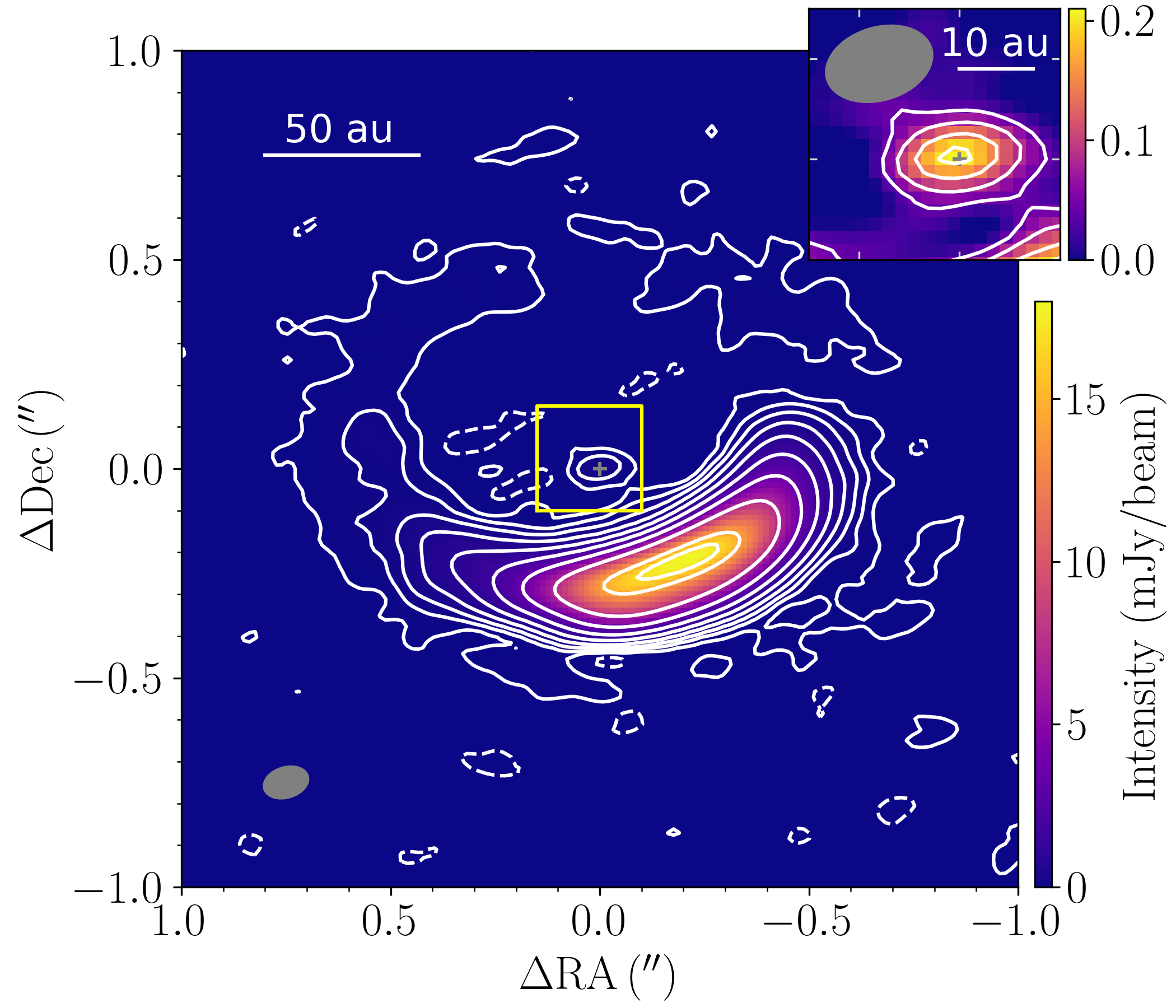
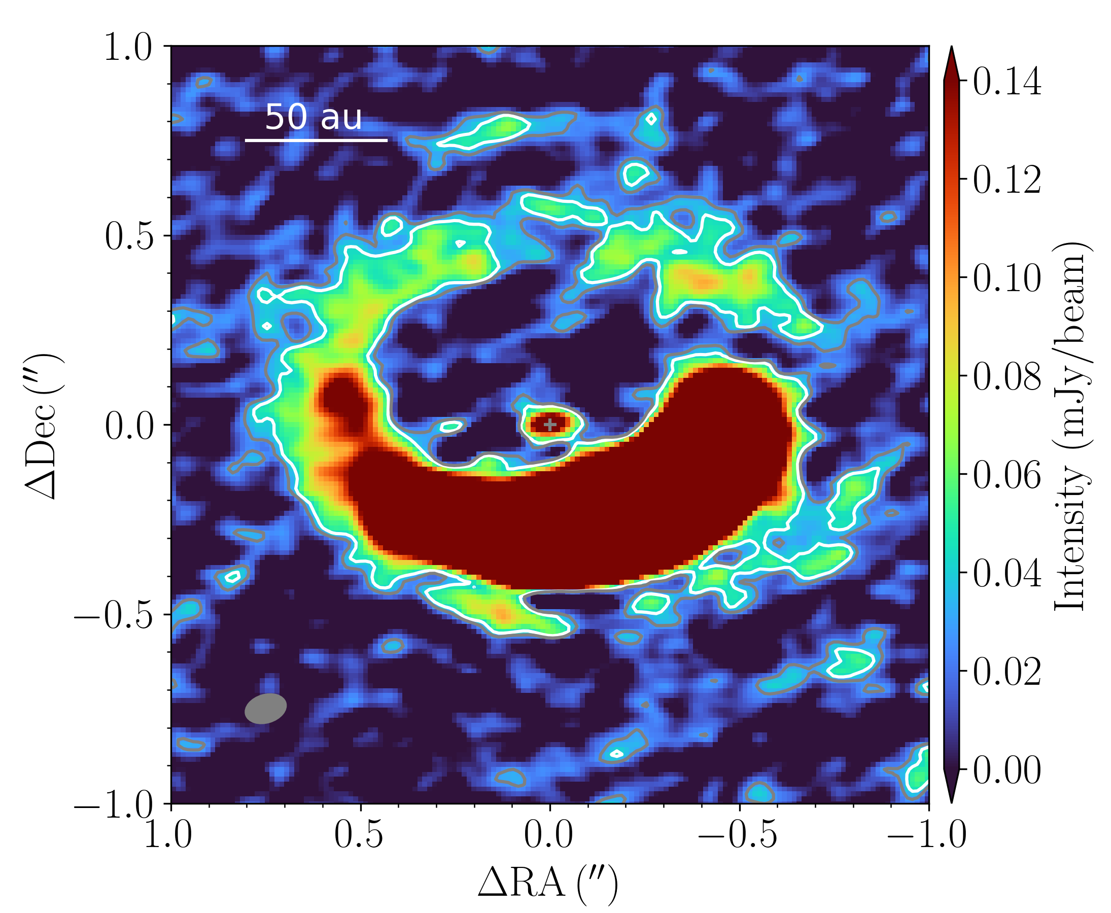
Figure 1: Left: The synthesized dust continuum image of IRS 48 at $870\rm\,\mu m$ or $345$ GHz. Both the colormap and the contours represent the flux density in mJy/beam. The contours are plotted at the levels of $(-3,3,8,16,64,128,256,512,1024,1200)\times\sigma$, where $\sigma=14\rm\,\mu Jy/beam$ is the rms noise. The synthesized beam is $0\farcs 11\times 0\farcs 072$. The inset shows a $0\farcs 15$ wide zoom, with contours representing the flux density at the levels of $(3,6,10,14)\times\sigma$. The star location is labeled as a gray cross. Right: The same image but with a different colormap with a maximum value $0.14\rm\,mJy/beam$, $10\sigma$, to saturate the crescent-shaped structure and display the dim long tail better. The white and gray contours correspond to flux densities of $3\sigma$ and $2\sigma$, respectively.

The primary-beam-corrected dust continuum image from our observation is shown in Fig. 1. The peak of the emission has $1285$ S/N or $18.00\rm\,mJy/beam$. In addition to the well-known crescent-shaped structure, we also detect a long tail of dust emission trailing behind the crescent-shaped structure, with respect to the counter-clockwise rotation of the disk (Bruderer et al., 2014), and some diffuse emission with over $3\sigma$ detection in the north west part of the disk. These two structures form an ellipse around the central object and will be discussed in Sec. 3.1. We also detect some emission at the $15\sigma$ level near the central object and separate it from the outer crescent for the first time. We will discuss this emission in Sec. 3.2.

3.1 Eccentric ring

Our ALMA observations are the deepest high resolution (sub)mm observations towards IRS 48 to date, reaching a noise level of $14\rm\,\mu Jy/beam$ at an angular resolution of $0\farcs 11\times 0\farcs 072$. For the first time we are able to significantly trace and detect emission from about $95\%$ of the ring crossing the crescent-shaped structure. Assuming an inclination angle of $50^{\circ}$ and a position angle of $100^{\circ}$ (Bruderer et al., 2014), we deproject the image to the disk plane. The results are shown in the left panel of Fig. 2. We can see that the north-northwest tail behind the crescent-shaped structure and the diffuse emission in the northwest part of the disk structure form an elliptical pattern rather than a circular pattern.

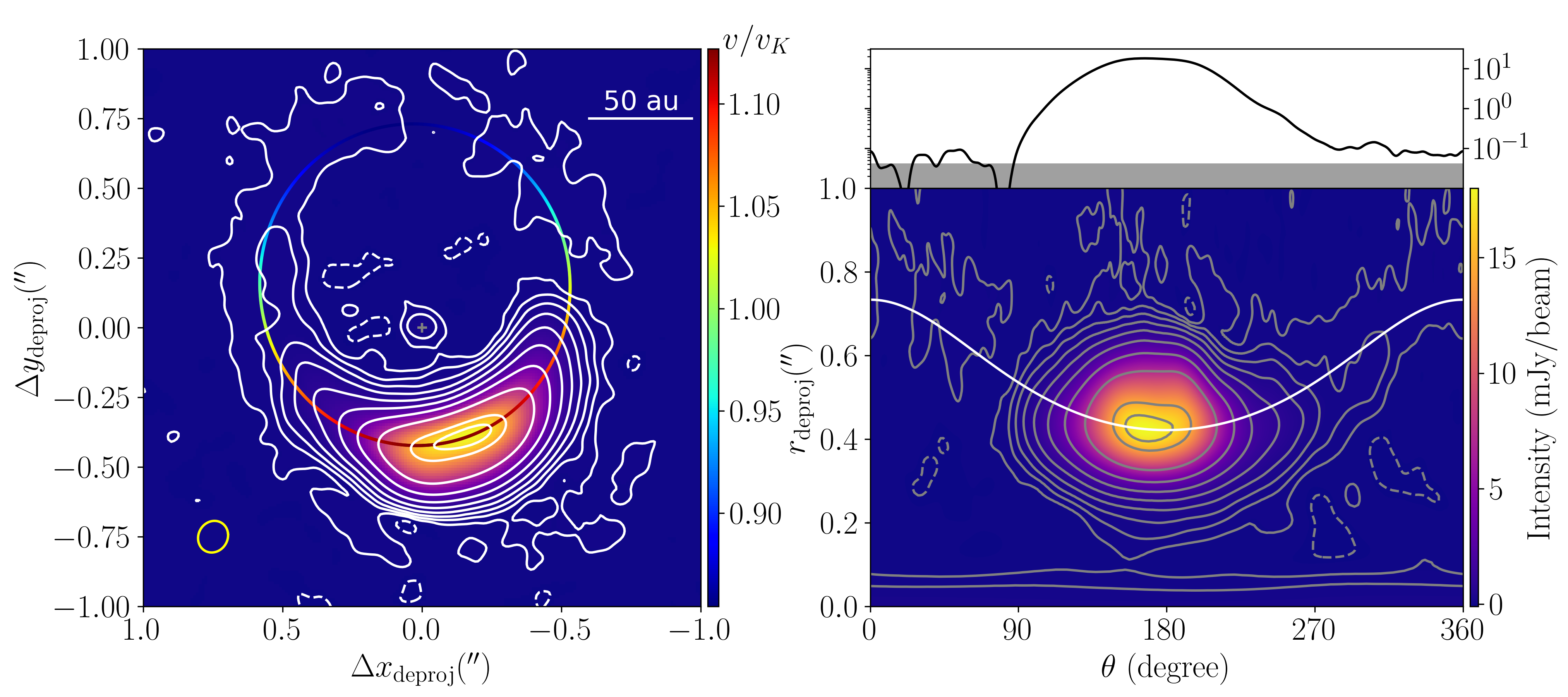
Figure 2: Left: The fitted elliptical ring in the deprojected view. The image shares the colorbar with the bottom right panel. The central star (gray cross; derived from Gaia DR3) is assumed to be one of the foci. The contours are plotted at the same levels as in Fig. 1. The colored ellipse shows the best fitted ring, with colors representing the ratio of the orbital velocity to the local Keplerian velocity, $v/v_{K}$ on the colorbar. The yellow ellipse at the lower left corner shows the synthetic beam deprojected to the disk plane. Bottom Right: The deprojected image in $(r,\theta)$ coordinates, where $\theta=0$ corresponds to the aphelion of the best fitted elliptical ring. Note that a circular orbit is a straight horizontal line in this view. Top Right: The flux density along the best fitted elliptical ring in logarithmatic scale. It shares the x-axis with the panel below. The gray contours are plotted at the same levels as in Fig. 1.

To fit the elliptical ring, we first parameterize the ellipse with the semi-major axis $a$, the eccentricity $e$, and the position angle of the major axis of the ellipse. We fix one of the foci on the central star. The fitting is done on the deprojected image, and the loss function is defined as $\mathcal{L}\equiv\sum I(x,y)f(dr(x,y))$, where $I(x,y)$ is the intensity and $dr(x,y)$ is the difference of the radial distance from the center between the point in the image and the target ellipse. The $f(dr)$ function is defined as:

$$f(dr)=\left\{\begin{array}[]{ll}(dr/\delta_{p})^{2}&\qquad dr\leq 0\\ (1.5dr/\delta_{p})^{2}&\qquad dr>0\end{array}\right.,$$ (1)

where $\delta_{p}=0\farcs 02$ is about the pixel size of our image, or $1/5$ of the beam size. The choice of $\delta_{p}$ and the pre-factor are arbitrary as we minimize the loss function to get the best fitted model. The loss function is engineered to have our fitted ellipse crossing the central peak of the crescent-shaped structure, as the one we present in the next paragraph.

The best fit is plotted as a colored ellipse in Fig. 2 with the color representing the ratio of the orbital velocity to the local Keplerian velocity $v/v_{K}$. The best fit has a semi-major axis $a=0.57^{\prime\prime}$, or $78$ au, and an eccentricity $e=0.27$. At the perihelion, the velocity is about $1.13v_{K}$, which is slightly super Keplerian. We will discuss the implication of the elliptical dust distribution in more detail in Sec. 4.1.

In the bottom right panel, we plot the same deprojected image in the $(r,\theta)$ coordinates. The $\theta$ is defined such that the perihelion corresponds to $\theta=180^{\circ}$. Note that a circular orbit is a horizontal straight line in these coordinates. Our fitted ellipse is very eccentric with an aphelion to perihelion distance ratio of $1.78$. In the top right panel, we plot the flux density profile in logarithmic scale along the fitted ellipse. We can see that the density structure is not symmetric with respect to the peak, and it resembles a droplet or a tadpole. The head is rounder with about $90^{\circ}$ degree spread in azimuthal angle whereas the tail spreads over almost $180^{\circ}$. The diffuse emission in the northwest part of the disk has an azimuthal extent of $40$-$50^{\circ}$. Since the emission along part of the ellipse is not robustly detected, the ratio of the maximum intensity is at least 400 times the minimum. As a reference for interested readers, the flux density contrast of the peak with the point along the ring with $180^{\circ}$ position angle difference is $271$.

The necessity for the ring to be eccentric is clear given that the north part is $\sim 1.8$ times further from the central star than the peak, and the exact value of the inclination angles does not change the eccentricity too much, as long as the position angle of the disk is fixed. From the left panel of Fig. 2, we can see that the major axis of the ellipse is very close to being vertical. In this case, changing the inclination angle will change both the apocenter and pericenter distances by the same factor, leaving the ratio unchanged as $\sim 1.8$. The semi-major axis will be different for the new inclination angle, but the eccentricity can be inferred directly as $e\approx(1.8-1)/(1.8+1)\approx 0.28$. So the eccentricity does not depend on the adopted inclination angle too much. The assumption of the central star as one focus has a much larger impact on the eccentricity. We will discuss these possibilities in more detail in Sec. 4.2.

3.2 Detection of central emission

Figure 1 clearly shows a central source with at least $3\sigma$ emission over more than $2$ beams. This source has a peak flux density of $0.21\rm\,mJy/beam$, at a signal-to-noise level $15\sigma$. We conduct a simple 2D-Gaussian fit to this central continuum emission. The center is only $3\rm\,mas$ west of the central star, well within one pixel of our image ($20$ mas). The spatial coincidence between the star location inferred from the Gaia data and the center of the central emission adds confidence to the location determination to both of them. It also makes it unlikely for this source to be either background contamination or random calibration or cleaning artifact. The major and minor axis of the 2D-Gaussian fit is $0.095^{\prime\prime}\times 0.052^{\prime\prime}$, which is smaller than our beam size. Even though the $3\sigma$ contour is larger than 2 beams, our data is still in agreement with a point source.

The simplest assumption is that this central emission comes from dust. However, before calculating a dust mass about the central source, we explore whether this emission may come from other sources. Firstly, the central emission cannot be completely explained by emission coming from a central star. The star IRS 48 was estimated as a $2\rm\,M_{\odot}$ star using kinematic modeling Brown et al. (2012). The effective temperature and the bolometric luminosity was estimated as $9520$ K and $17.8\rm\,L_{\odot}$ (Brown et al. 2012; rescaled by Francis & van der Marel (2020) using new distance from Gaia DR2 data (Gaia Collaboration et al., 2018)). The effective temperature and the bolometric luminosity combined yield a radius of $1.55\rm\,R_{\odot}$. We can then calculate the flux density at the wavelength of $870\rm\,\mu m$ as $7.22\times 10^{-6}\rm\,Jy$. This is $21$ times smaller than what we detect.

Another possibility to explain the central unresolved emission is that it comes from the free-free emission of an ionized wind. Taking the flux of the central source at 34 GHz ($36\rm\,\mu$Jy, van der Marel et al. 2015) and the flux derived in our 2D-Gaussian fit at 343.5 GHz ($221\rm\,\mu$Jy), we obtain a spectral index of $0.78\pm 0.20$. This spectral index is consistent with the partially optically thick free-free emission of a jet/wind. Although ionized jets are common among young stars the turnover frequency from the partially optically thick to the optically thin regimes depends upon the ionized gas density at the jet base and it is usually located at the centimeter part of the continuum spectrum (e.g., Reynolds, 1986; Mohan et al., 2022). Therefore, if the emission of the central source at 343.5 GHz has a contribution from a thermal ionized jet, it would most probably be in the optically thin regime, with a spectral index of $-0.1$. Assuming that the emission of a thermal jet is optically thin from 34 to 343.5 GHz, the free-free contribution would be $29\mu$Jy at 343.5 GHz, roughly 10 times smaller than the measured flux.

Neither the emission from the protostellar photosphere, nor the emission from an ionized wind could alone (or added) explain the measured flux from the central source in the ALMA image. Still other possible contributions can be due to the non-thermal synchrotron emission from the protostellar magnetosphere (Andre & Yau, 1997), the ionized emission from the dust sublimation wall (e.g., Añez-López et al., 2020), or the collisions from pebbles and planetesimals that heat the dust of a disk (such as proposed in Vega, Matrà et al., 2020). The former two hypotheses are expected to be more prominent in the centimeter wavelength range, while the third hypothesis is somehow a more exotic solution that may need more theoretical work to be supported. In this work we will assume a more simple hypothesis, in which most of the submillimeter emission comes from the thermal dust emission of an inner disk. Following this idea, we can put a constraint on the dust mass of the central object. The mean flux density within the $3\sigma$ contour is about $8.65\times 10^{-5}\rm\,Jy/beam$, corresponding to a brightness temperature of $0.164$ K. This is extremely optically thin for any reasonable dust temperature. The area of this region is measured as $291\rm\,au^{2}$. Given the small size of the central source (maximum distance from the central star is $\sim 10$ au), we assume a dust temperature of $100$ K. We also assume a dust opacity of $3.5\rm\,cm^{2}/g$, which is the fiducial dust model from Birnstiel et al. (2018) with $1$ mm maximum grain size at $870\rm\,\mu m$ wavelength. Under these assumptions, the dust mass is estimated to be about $1.5\times 10^{-8}M_{\odot}$, or $0.005\rm\,M_{\oplus}$.

4 Discussion

4.1 Proper motion

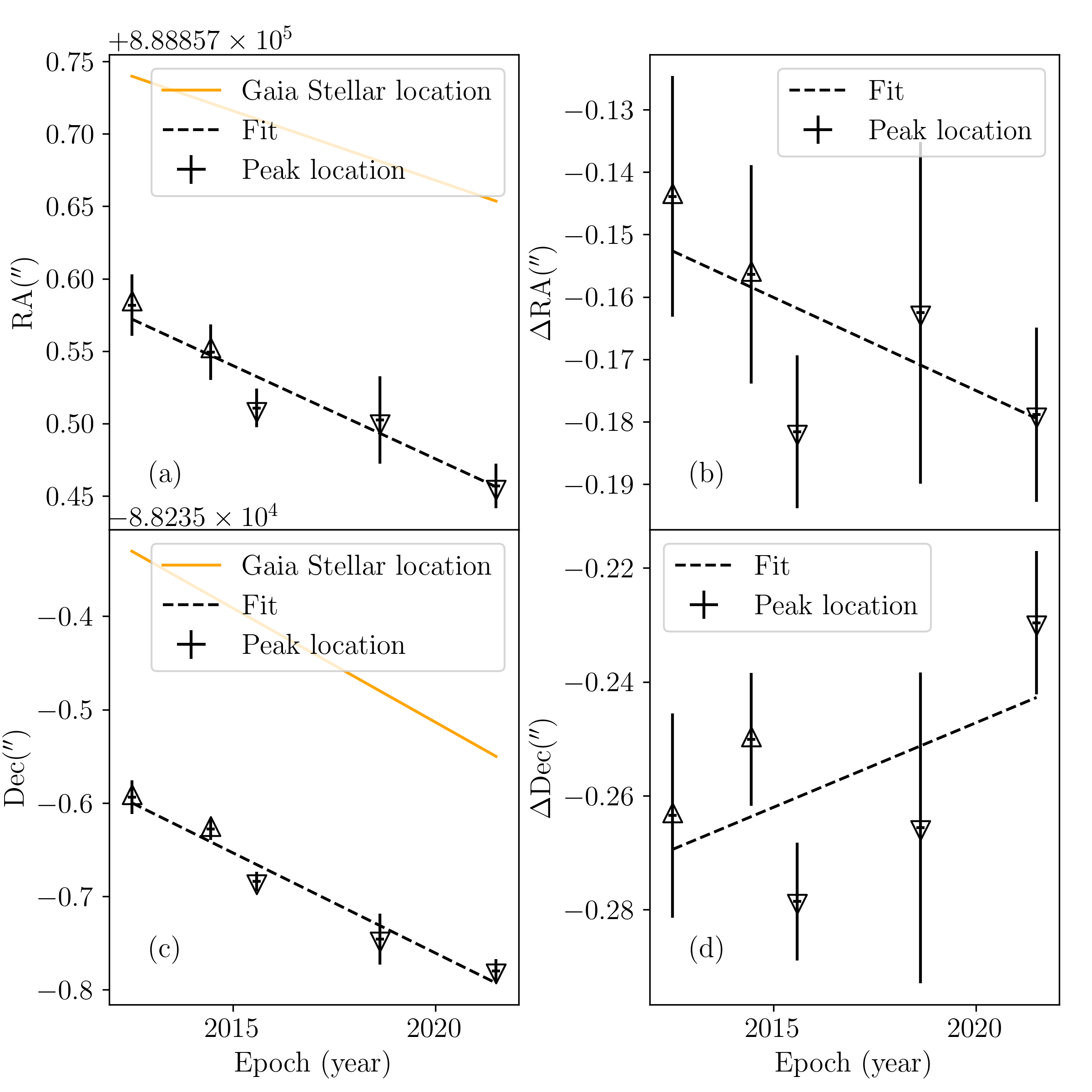
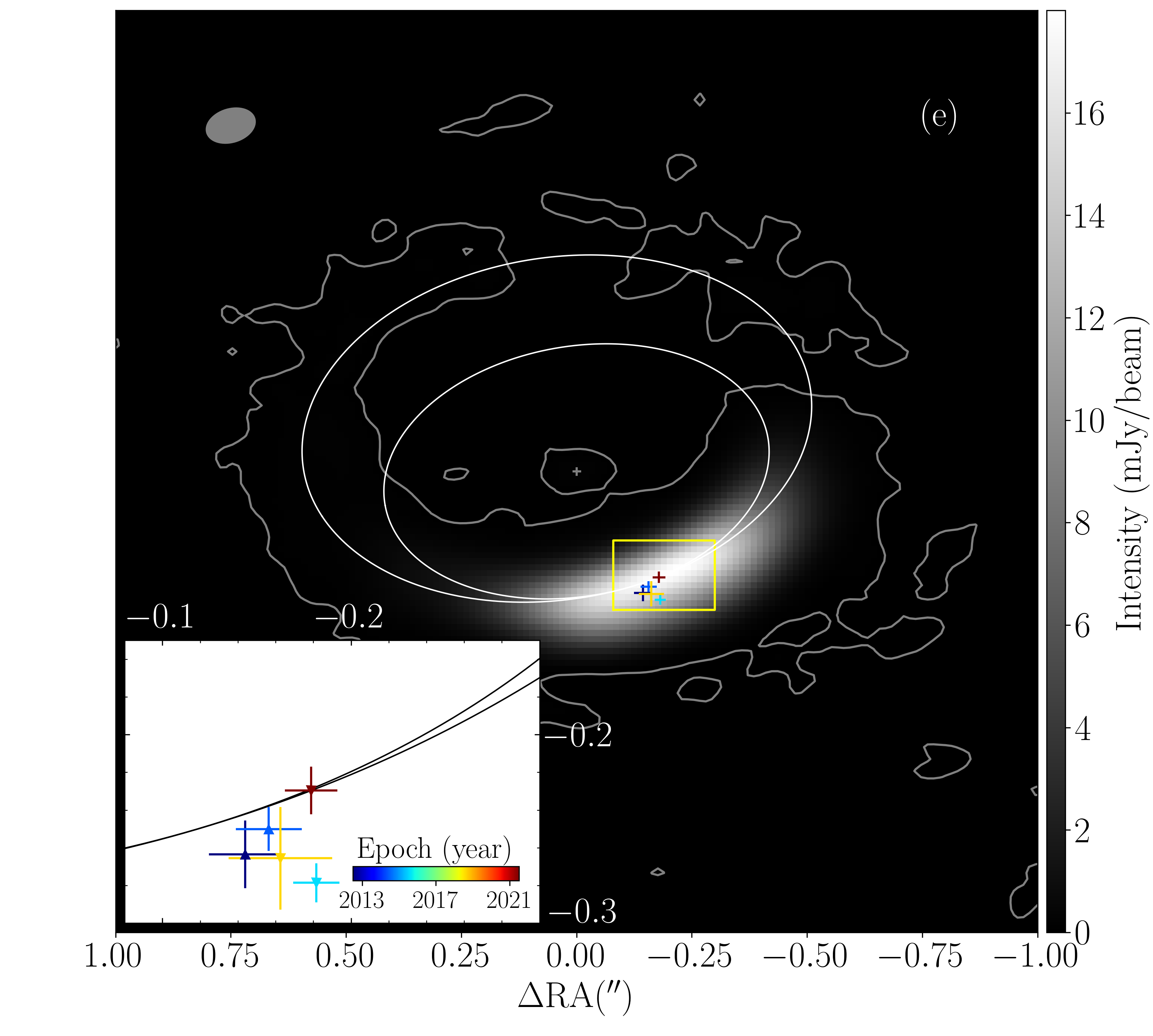
Figure 3: The Right Ascension (a) and Declination (c) of the crescent peak from archival ALMA data and the star assuming Gaia proper motion in units of arcsec. The relative displacement from the assumed stellar location at each epoch is plotted in unit of arcsec in (b) and (d). The dashed lines are linear fits to each data sets. The up (down) triangles represent data points observed at ALMA Band 9 (Band 7). Panel (e): The intensity image overlaid with the predicted proper motion. The smaller and larger ellipses represent the circular and the best fit eccentric orbit, respectively. The colorful crosses represent the fitted peak location at each epochs with errors.

In Sec. 3.1, we fit the ring crossing the crescent-shaped structure with an elliptical orbit having an eccentricity of $0.27$, and the current peak of the crescent-shaped structure is near the perihelion of the orbit. Such an eccentric orbit would have a local velocity near the perihelion of about $1.13v_{K}$. The crescent-shaped structure following this orbit should also move at a super Keplerian speed.

Since van der Marel et al. (2013), the IRS 48 has been observed with ALMA at high resolution multiple times (van der Marel et al. 2015; Francis & van der Marel 2020; van der Marel et al. 2021a; 2021 observations in this study). The 9 year separation in observing time allows us to constrain the proper motion of the crescent-shaped structure. We obtained the archival ALMA data and use CASA imfit to conduct 2D Gaussian fit to the crescent. The observation time, adopted epoch, observing band, beam size, astrometric error $\delta_{\mathrm{astro}}$, imfit results, and references are presented in Table 1. When estimating the astrometric error, we followed the ALMA Technical Handbook, which is the beam size divided by the signal to noise ratio (saturates in $20$) divided by 0.9. For observations with resolution finer than $0\farcs 15$, the positional error can be up to a factor of two higher. Only our observations are this high resolution, so we doubled the aforementioned astrometric error to be conservative. For the imfit results, we present the fitted peak location translated to the ICRS frame, the error in RA and the error in Dec. The locations of the peaks are plotted in panels (a) and (c) in Figure 3. The errors in fitted RA and Dec are the square root of the sum of the squared errors from both astrometric error and fitting error. We also put $0.1$ error for all epoches, which is on the order of one month. The stellar location from the Gaia proper motion measurement is also plotted, which allows us to calculate the relative displacement from the central star in panels (b) and (d). We do not consider the astrometric error from Gaia.

Observation time	Epoch	Band	Beam size	$\delta_{\mathrm{astro}}(^{\prime\prime})$	Peak Location (ICRS)	$\delta_{\mathrm{RA}}(^{\prime\prime})$	$\delta_{\mathrm{Dec}}(^{\prime\prime})$	Refs
06/2012; 07/2012	2012.50	9	$0\farcs 32\times 0\farcs 21$	0.018	$16^{\rm h}27^{\rm m}37\mbox{${}^{\rm s}\mskip-7.6mu.\,$}172$, $-24^{\circ}30^{\prime}35\mbox{${}^{\prime\prime}\mskip-7.6mu.\,$}593$	0.0075	0.0024	1
06/2014	2014.45	9	$0\farcs 19\times 0\farcs 14$	0.011	$16^{\rm h}27^{\rm m}37\mbox{${}^{\rm s}\mskip-7.6mu.\,$}169$, $-24^{\circ}30^{\prime}35\mbox{${}^{\prime\prime}\mskip-7.6mu.\,$}628$	0.0139	0.0049	2
07/2015; 08/2015	2015.58	7	$0\farcs 18\times 0\farcs 12$	0.010	$16^{\rm h}27^{\rm m}37\mbox{${}^{\rm s}\mskip-7.6mu.\,$}167$, $-24^{\circ}30^{\prime}35\mbox{${}^{\prime\prime}\mskip-7.6mu.\,$}684$	0.0070	0.0026	3
08/2018	2018.63	7	$0\farcs 49\times 0\farcs 39$	0.027	$16^{\rm h}27^{\rm m}37\mbox{${}^{\rm s}\mskip-7.6mu.\,$}166$, $-24^{\circ}30^{\prime}35\mbox{${}^{\prime\prime}\mskip-7.6mu.\,$}745$	0.0031	0.0015	4
06/2021; 07/2021	2021.50	7	$0\farcs 11\times 0\farcs 072$	0.012	$16^{\rm h}27^{\rm m}37\mbox{${}^{\rm s}\mskip-7.6mu.\,$}163$, $-24^{\circ}30^{\prime}35\mbox{${}^{\prime\prime}\mskip-7.6mu.\,$}779$	0.0068	0.0030	5

Table 1: The proper motion of the peak of the crescent-shaped structure. $\delta_{\mathrm{astro}}$ is the astrometric error. $\delta_{\mathrm{RA}}$ and $\delta_{\mathrm{Dec}}$ are fitting error using imfit for RA and Dec, respectively. The references and ALMA project IDs are: (1) van der Marel et al. (2013),2011.0.00635.SSB; (2) van der Marel et al. (2015), 2013.1.00100.S; (3) Francis & van der Marel (2020), van der Marel et al. (2021b), 2013.1.00100.S; (4) Ohashi et al. (2020), van der Marel et al. (2021a), 2017.1.00834.S; (5) This work, 2019.1.01059.S.

We note that the first two points, from van der Marel et al. (2013) and van der Marel et al. (2015), are observed at Band 9 ($440\rm\,\mu m$), whereas the others are observed at Band 7 ($870\rm\,\mu m$). Since the peak at $440\rm\,\mu m$ was reported to coincide with that at 9 mm van der Marel et al. (2015), it is reasonable to ignore the potential azimuthal displacement here, even though it was predicted in simulations with self gravity (Baruteau & Zhu, 2016). We will use all 5 data points to fit the proper motion for larger sample size and time span. To highlight the difference in observing bands, we have marked the data observed at Band 9 and Band 7 with up triangles and down triangles, respectively, in all panels of Figure 3.

With these caveats in mind, we fit the proper motion of the peak after subtracting the stellar proper motion as $(-3.0\pm 1.9,3.0\pm 2.5)\rm\,mas/yr$. This is $(-1.9\pm 1.2,1.9\pm 1.6)\rm\,km/s$ at a distance of $136\rm\,pc$ and $(-0.35\pm 0.22,0.35\pm 0.29)\times v_{K}$, where as $v_{K}=5.438\rm\,km/s$ is the Keplerian velocity at the distance of $60$ au, the location of the peak. The magnitude of the proper motion is $0.49\pm 0.26\,v_{K}$.

In panel (e) of Fig. 3, we over plot the circular orbit and the best-fit elliptical orbit on the image. We also plot the peak locations as colorful dots with colors representing their observing epoch. We can see that the data points do not follow either a circular orbit or an eccentric orbit. There are a few possibilities that may cause this mismatch. For example, in the case of an undetected stellar companion with a non-negligible mass (as suggested by Calcino et al. 2019), the Gaia proper motions do not take into account the possible orbital motion of the primary star. It is also possible that the crescent peak has some epicycle motion in addition to bulk orbital motion. Further work with all datasets modeled more accurately and consistently and observations towards the IRS 48 with high resolution again in $5-10$ years may help to understand the nature of the proper motion of the crescent peak.

4.2 Secondary stellar companion?

Theoretically, one way to drive the eccentric orbital motion is to have a secondary stellar companion. In the simulation presented in Calcino et al. (2019), they introduced a companion as massive as $0.4\rm\,M_{\odot}$ at the separation of $10$ au, to explain the observed asymmetry in velocity channel maps and line observations (van der Marel et al., 2016). Such a massive companion will change the mass center of the system significantly ($1.67$ au for their set-up), and the focus of the eccentric ring should be displaced from the central star.

To explore these possibilities, we relax the constraint in Sec. 3.1 and introduce the location of the focus as two additional parameters. The loss function is still defined with the difference between the distances towards the new focus as its argument. There are many ellipses with similar levels of loss functions. In Fig. 4, we plot $1000$ orbits and their foci with reasonable fits to our data. Among these ellipses, the largest loss function is only $\sim 1\%$ larger than the smallest one. Despite the similarity in their loss functions, the location of the foci differs by almost $50$ au.

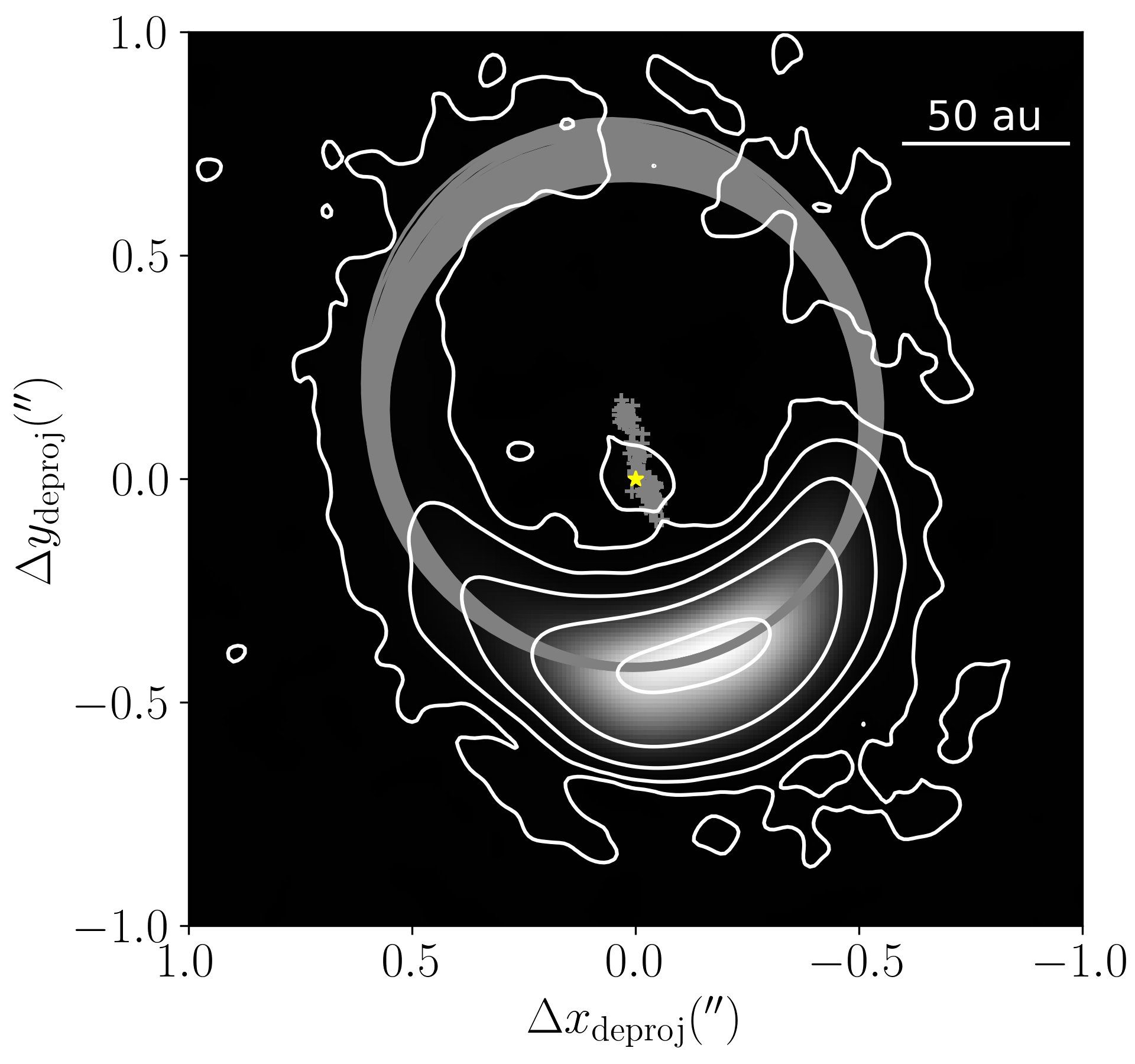
Figure 4: Orbital fits shown in the deprojected plane without using the assumption of the star at one of the foci. We plot $1000$ gray ellipses with a reasonable fit. The worst of these orbits has a loss function that is only $1\%$ larger than the best. The foci (near the star) of these ellipses are also plotted as gray crosses. The yellow star at the center marks the primary star location.

The uncertainty of the fitted focus mostly comes from the dispersed nature of the emission. Deeper observations with lower noise are unlikely to give much better constraints. Aside from constraints from the dust emission, one can search for the potential secondary star with astrometry, in addition to the existing constraint from photometry (Wright et al. 2015, c.f. discussions by Calcino et al. 2019). If there is a massive secondary stellar companion, the proper motion of the central star should have an oscillating component on the order of $1.5-2$ au. If the orbit is significantly inclined, we should also observe a radial variance ($\sim 1.8\rm\,km/s$ if the inclination is the same as the disk) with a period of about $20$ years.

Note that the discussion on the secondary stellar companion and the displaced focus will change the proper motion discussed earlier. The Keplerian velocity will change with a different total mass of the central binary system and with a different distance to the displaced focus. The system may not be super Keplerian anymore if the total stellar mass is larger. More detailed future analyses are needed to account for these additional complications.

4.3 Velocity maps of line emissions

The elliptical orbit also has an impact on the velocity maps of line emission, assuming the gas is co-moving with the dust. The velocity map with an eccentricity of $e=0.27$ from our best-fit model is shown in Fig. 5. We adopt a systemic velocity of 4.55 km/s as in van der Marel et al. (2021a) and the resulting velocity map is similar to their Fig. 1. In order to compare with Keplerian rotation, we also plot the iso-velocity contours for the elliptical orbit as black solid lines and the contours with same levels for Keplerian rotation as black dashed lines. We can see that the red region is significantly larger than the blue region, and the red-shifted solid contours are larger than their blue-shifted counterparts. This is in contrast with the circular orbit, where the dashed red-shifted contours are similar in sizes to the dashed blue-shifted contours. This is because the western part of the disk is closer to the perihelion and will show larger velocities in an elliptical orbit. This asymmetry that the red-shifted contours are larger than their blue-shifted counterparts in velocity maps is visible in both $\rm H_{2}CO$ and $\rm{}^{13}CO$ (van der Marel et al., 2014, 2021a), which lends support to the elliptical orbit (as first discussed by Calcino et al. 2019), although it remains to be determined whether the velocity map is quantitatively consistent with the eccentricity of $e=0.27$ inferred from the dust emission distribution.

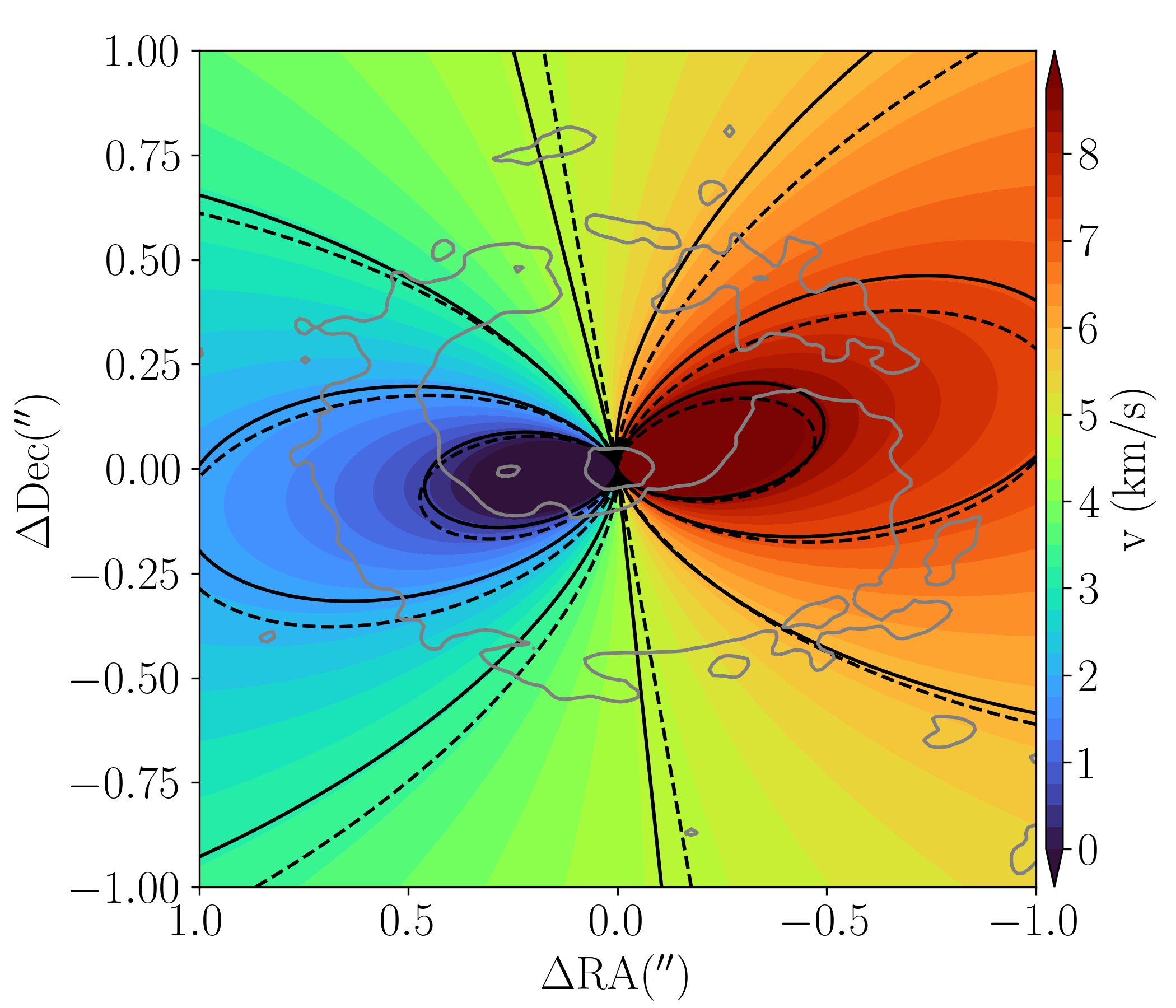
Figure 5: The velocity map of the disk, assuming an elliptical orbit with $e=0.27$, as fitted from Sec. 3.1. The colorbar is similar to van der Marel et al. (2021a) with $v_{\mathrm{source}}=4.55\rm\,km/s$. The solid contours represent the same velocity map as the color map at the levels of $(-4,-2.67,-1.33,0,1.33,2.67,4)\rm\,km/s+v_{\mathrm{source}}$. The dashed contours are plotted at the same velocity levels but assumes circular (Keplerian) orbit. A gray $3\sigma$ contour of the non-polarized flux from our observation is also plotted as a background.

5 Summary

In this work, we present deep submillimeter ALMA observations towards the transition disk IRS 48 with a high spatial resolution. The main findings are as follows:

1. For the first time, we are able to trace $95\%$ of the ring crossing the well-known crescent-shaped structure. This ring is surprisingly eccentric with a large eccentricity of $0.27$.

2. We detected compact emission at 15 $\sigma$ level that is centered in the star and spatially well separate from the crescent-shaped structure. The dust mass is estimated as about $1.5\times 10^{-8}\rm\,M_{\odot}$, or $0.005\rm\,M_{\oplus}$, if the emission is mm-sized dust thermal emission. We do not resolve the central emission with $0.1^{\prime\prime}$ beam. If the central object is an unresolved inner disk, the disk radius is a couple of astronomical units at most.

3. We fit the proper motion of the crescent-shaped dust structure as $0.49\pm 0.26\,v_{K}$. Existing data do not support either circular orbit or elliptical orbit. Detailed modeling and future high-resolution observations may help to understand the nature of the proper motion of the crescent peak.

References

- Añez-López et al. (2020) Añez-López, N., Osorio, M., Busquet, G., et al. 2020, ApJ, 888, 41, doi: 10.3847/1538-4357/ab5dbc
- Alexander et al. (2014) Alexander, R., Pascucci, I., Andrews, S., Armitage, P., & Cieza, L. 2014, in Protostars and Planets VI, ed. H. Beuther, R. S. Klessen, C. P. Dullemond, & T. Henning, 475, doi: 10.2458/azu_uapress_9780816531240-ch021
- Andre & Yau (1997) Andre, M., & Yau, A. 1997, Space Sci. Rev., 80, 27, doi: 10.1023/A:1004921619885
- Ataiee et al. (2013) Ataiee, S., Pinilla, P., Zsom, A., et al. 2013, A&A, 553, L3, doi: 10.1051/0004-6361/201321125
- Baruteau & Zhu (2016) Baruteau, C., & Zhu, Z. 2016, MNRAS, 458, 3927, doi: 10.1093/mnras/stv2527
- Birnstiel et al. (2013) Birnstiel, T., Dullemond, C. P., & Pinilla, P. 2013, A&A, 550, L8, doi: 10.1051/0004-6361/201220847
- Birnstiel et al. (2018) Birnstiel, T., Dullemond, C. P., Zhu, Z., et al. 2018, ApJ, 869, L45, doi: 10.3847/2041-8213/aaf743
- Brown et al. (2012) Brown, J. M., Herczeg, G. J., Pontoppidan, K. M., & van Dishoeck, E. F. 2012, ApJ, 744, 116, doi: 10.1088/0004-637X/744/2/116
- Bruderer et al. (2014) Bruderer, S., van der Marel, N., van Dishoeck, E. F., & van Kempen, T. A. 2014, A&A, 562, A26, doi: 10.1051/0004-6361/201322857
- Calcino et al. (2019) Calcino, J., Price, D. J., Pinte, C., et al. 2019, MNRAS, 490, 2579, doi: 10.1093/mnras/stz2770
- Dong et al. (2018) Dong, R., Li, S., Chiang, E., & Li, H. 2018, ApJ, 866, 110, doi: 10.3847/1538-4357/aadadd
- Espaillat et al. (2010) Espaillat, C., D’Alessio, P., Hernández, J., et al. 2010, ApJ, 717, 441, doi: 10.1088/0004-637X/717/1/441
- Espaillat et al. (2014) Espaillat, C., Muzerolle, J., Najita, J., et al. 2014, in Protostars and Planets VI, ed. H. Beuther, R. S. Klessen, C. P. Dullemond, & T. Henning, 497, doi: 10.2458/azu_uapress_9780816531240-ch022
- Francis & van der Marel (2020) Francis, L., & van der Marel, N. 2020, ApJ, 892, 111, doi: 10.3847/1538-4357/ab7b63
- Gaia Collaboration et al. (2018) Gaia Collaboration, Brown, A. G. A., Vallenari, A., et al. 2018, A&A, 616, A1, doi: 10.1051/0004-6361/201833051
- Gaia Collaboration et al. (2022) Gaia Collaboration, Vallenari, A., Brown, A. G. A., et al. 2022, arXiv e-prints, arXiv:2208.00211. https://arxiv.org/abs/2208.00211
- Geers et al. (2007) Geers, V. C., Pontoppidan, K. M., van Dishoeck, E. F., et al. 2007, A&A, 469, L35, doi: 10.1051/0004-6361:20077524
- Kley & Dirksen (2006) Kley, W., & Dirksen, G. 2006, A&A, 447, 369, doi: 10.1051/0004-6361:20053914
- Marsh & Mahoney (1992) Marsh, K. A., & Mahoney, M. J. 1992, ApJ, 395, L115, doi: 10.1086/186501
- Matrà et al. (2020) Matrà, L., Dent, W. R. F., Wilner, D. J., et al. 2020, ApJ, 898, 146, doi: 10.3847/1538-4357/aba0a4
- McMullin et al. (2007) McMullin, J. P., Waters, B., Schiebel, D., Young, W., & Golap, K. 2007, in Astronomical Society of the Pacific Conference Series, Vol. 376, Astronomical Data Analysis Software and Systems XVI, ed. R. A. Shaw, F. Hill, & D. J. Bell, 127
- Mohan et al. (2022) Mohan, S., Vig, S., & Mandal, S. 2022, MNRAS, 514, 3709, doi: 10.1093/mnras/stac1159
- Ohashi et al. (2020) Ohashi, S., Kataoka, A., van der Marel, N., et al. 2020, ApJ, 900, 81, doi: 10.3847/1538-4357/abaab4
- Ragusa et al. (2020) Ragusa, E., Alexander, R., Calcino, J., Hirsh, K., & Price, D. J. 2020, MNRAS, 499, 3362, doi: 10.1093/mnras/staa2954
- Ragusa et al. (2017) Ragusa, E., Dipierro, G., Lodato, G., Laibe, G., & Price, D. J. 2017, MNRAS, 464, 1449, doi: 10.1093/mnras/stw2456
- Reynolds (1986) Reynolds, S. P. 1986, ApJ, 304, 713, doi: 10.1086/164209
- Salyk et al. (2013) Salyk, C., Herczeg, G. J., Brown, J. M., et al. 2013, The Astrophysical Journal, 769, 21, doi: 10.1088/0004-637X/769/1/21
- van der Marel et al. (2021a) van der Marel, N., Booth, A. S., Leemker, M., van Dishoeck, E. F., & Ohashi, S. 2021a, A&A, 651, L5, doi: 10.1051/0004-6361/202141051
- van der Marel et al. (2015) van der Marel, N., Pinilla, P., Tobin, J., et al. 2015, ApJ, 810, L7, doi: 10.1088/2041-8205/810/1/L7
- van der Marel et al. (2016) van der Marel, N., van Dishoeck, E. F., Bruderer, S., et al. 2016, A&A, 585, A58, doi: 10.1051/0004-6361/201526988
- van der Marel et al. (2014) van der Marel, N., van Dishoeck, E. F., Bruderer, S., & van Kempen, T. A. 2014, A&A, 563, A113, doi: 10.1051/0004-6361/201322960
- van der Marel et al. (2013) van der Marel, N., van Dishoeck, E. F., Bruderer, S., et al. 2013, Science, 340, 1199, doi: 10.1126/science.1236770
- van der Marel et al. (2021b) van der Marel, N., Birnstiel, T., Garufi, A., et al. 2021b, AJ, 161, 33, doi: 10.3847/1538-3881/abc3ba
- Wright et al. (2015) Wright, C. M., Maddison, S. T., Wilner, D. J., et al. 2015, MNRAS, 453, 414, doi: 10.1093/mnras/stv1619
- Zhu et al. (2014) Zhu, Z., Stone, J. M., Rafikov, R. R., & Bai, X.-n. 2014, ApJ, 785, 122, doi: 10.1088/0004-637X/785/2/122