Vortex phase matching of a self-propelled model of fish with autonomous fin motion

Abstract

It has been a long-standing problem how schooling fish optimize their motion by exploiting the vortices shed by the others. A recent experimental study showed that a pair of fish reduce energy consumption by matching the phases of their tailbeat according to their distance. In order to elucidate the dynamical mechanism by which fish control the motion of caudal fins via vortex-mediated hydrodynamic interactions, we introduce a new model of a self-propelled swimmer with an active flapping plate. The model incorporates the role of the central pattern generator network that generates rhythmic but noisy activity of the caudal muscle, in addition to hydrodynamic and elastic torques on the fin. For a solitary fish, the model reproduces a linear relation between the swimming speed and tailbeat frequency, as well as the distributions of the speed, tailbeat amplitude, and frequency. For a pair of fish, both the distribution function and energy dissipation rate exhibit periodic patterns as functions of the front-back distance and phase difference of the flapping motion. We show that a pair of fish spontaneously adjust their distance and phase difference via hydrodynamic interaction to reduce energy consumption.

I Introduction

Collective behavior of biological units such as insects, birds, mammals and fish are ubiquitously found in Nature and have attracted attention for many years Conradt2005 ; Vicsek2012 . Schooling fish exhibit various patterns of collective motion Parrish2002 ; Lopez2012 ; Terayama2015 , for avoiding predators Parrish2002 , foraging food Harpaz2020 , and reducing hydrodynamic cost of swimming Liao2007 . They have been studied by agent-based models that regard an individual fish as a self-propelled particle with positional and orientational degrees of freedom Breder1954 ; Aoki1982 ; Huth1992 ; Huth1994 ; Niwa1994 ; Couzin2002 ; Hemelrijk2008 ; Gautrais2012 ; Calovi2014 ; Bastien2020 ; Ito2022a ; Ito2022b ; Tchieu2012 ; Gazzola2016 ; Filella2018 ; Deng2021 . Interactions between fish are modeled by a potential Breder1954 ; Niwa1994 or zones with a blind angle Aoki1982 ; Couzin2002 ; Huth1992 ; Huth1994 , while recent works incorporate topological interactions Gautrais2012 ; Calovi2014 ; Filella2018 ; Deng2021 ; Ito2022a ; Ito2022b , gravity sensing Hemelrijk2008 ; Ito2022b , and visual information Bastien2020 . Hydrodynamic interactions are taken into account by time-averaged dipolar flow Tchieu2012 ; Gazzola2016 ; Filella2018 ; Deng2021 . However, the self-propelled particle models do not describe the motion of caudal fins, which is matched to the vortex flow to reduce muscle activity Liao2007 .

An undulating caudal fin sheds a reverse Kármán vortex street, whose vorticity has an opposite sign compared to a Kármán vortex street Lauder2002 ; Akanyeti2017 ; Wise2018 . It has long been hypothesized that schooling fish exploit the reverse Kármán vortex to reduce energy consumption Breder1965 ; Weihs1973 . Weihs proposed that fish form a two-dimensional diamond lattice structure to reduce hydrodynamical drag force caused by the vortices Weihs1973 . Later observations on some species of fish, however, demonstrated that a fish school does not preserve a specific lattice structure Partridge1979 ; Marras2014 . More recent experiments revealed that red nose tetra (Hemigrammus bleheri) synchronize their tailbeat with the nearest neighbors at high swimming speed Ashraf2016 ; Ashraf2017 . Li et al. Li2020 found a linear relation between the phase difference of the tailbeat and the front-back distance between a pair of goldfish (Carassius auratus), which shows that the motion of the caudal fins are regulated by the periodicity of the vortices and weakly phase-locked at any short distance. Using robotic fish, they also found that energy consumption is reduced by matching the phases of the vortices generated by two fish Li2020 . These results indicate the necessity of a theoretical model that describes autonomous motion and phase locking of caudal fins. Since hydrodynamic synchronization does not necessarily lead to minimization of energy dissipation Elfring2009 ; Liao2021 , the dynamical mechanism exploited by fish to reduce energy consumption is highly nontrivial.

Previous models of vortex-mediated interaction between fish use (i) flapping Dewey2014 ; Boschitsch2014 or heaving Becker2015 ; Ramananarivo2016 ; Newbolt2019 ; Oza2019 airfoils, (ii) elastic filaments Zhu2014 ; Park2018 ; Peng2018 , or (iii) deformable fish-shaped swimmers Hemelrijk2015 ; Daghooghi2015 ; Maertens2017 ; Li2019 ; XLi2021 ; Pan2022 ; Kelly2023 ; Lin2023 . The type (i) models allow analytical treatment by Joukowski transformation Dewey2014 ; Ramananarivo2016 ; Oza2019 and direct comparison with experiments Dewey2014 ; Boschitsch2014 ; Becker2015 . Computational fluid dynamics simulations are employed for the type (ii) and (iii) models. The type (ii) models treat hydroelastic deformation of the filament in two dimensions induced by prescribed oscillation of the filament head. The type (iii) models prescribe undulatory motion of a three-dimensional fish-shaped body. Optimal swimming patterns are discussed for two bodies Dewey2014 ; Boschitsch2014 ; Becker2015 ; Ramananarivo2016 ; Newbolt2019 ; Maertens2017 ; Li2019 ; Zhu2014 ; Peng2018 ; Lin2023 and a lattice Hemelrijk2015 ; Daghooghi2015 ; Oza2019 ; Park2018 ; XLi2021 ; Pan2022 ; Kelly2023 of fish. Some studies incorporate temporal evolution of the distance between swimmers Ramananarivo2016 ; Newbolt2019 ; Zhu2014 ; Park2018 ; Peng2018 , but the phases of the oscillation or undulation are prescribed in all the models.

In this paper, we introduce a minimal but integrated model of fish that self-propels by autonomous fin motion and interacts via a reverse Kármán vortex street. By incorporating physiological noises in the signals transmitted to the caudal muscle, the model describes spontaneous time evolution of the phase of the caudal fin, which is modeled by an active flapping plate. The noises are essential in reproducing the distribution of the swimming speed of a solitary swimmer and the vortex-mediated correlation between the distance and phases of two swimmers that are experimentally observed Li2020 .

This paper is organized as follows. In Sect. II, we construct the model incorporating hydrodynamical forces, elasticity of the caudal fin, and an active physiological noises. In Sect. III, to test the validity of the model, we analyze the properties of solitary swimming and compare them with experimental results. In Sect. IV, we consider a pair of swimmers and show that the correlation between their distance and phase difference reflects the periodicity of the vortices. We also show that the fish tend to be distributed at short distances where they adjust their phase difference to reduce energy dissipation. We discuss the results in comparison with previous studies in Sect. V.

II Flapping plate model

II.1 Equations of motion and forces

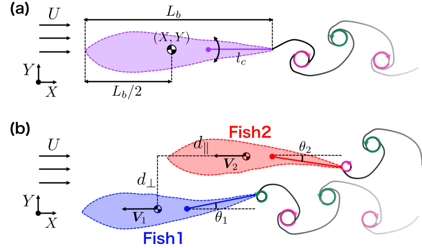
Figure 1: Schematic illustration of (a) a solitary swimmer and (b) a pair of swimmers. The swimmers are placed in a uniform background flow of speed $U$ along the $X$-direction. In (a), the center of the swimmer is at $(X,Y,0)$. The right top inset shows the swimmer viewed from the side. The configuration of a pair of swimmers is specified by the longitudinal distance $d_{\parallel}=|X_{1}-X_{2}|$, the lateral distance $d_{\perp}=|Y_{1}-Y_{2}|$ and the angles $\theta_{1}$, $\theta_{2}$ of the flapping plates. (In the figure, $\theta_{1}>0$ and $\theta_{2}<0$). The vortices shedded by the swimmers are carried away by the background flow and diminish.

The modes of fish locomotion are classified into anguilliform, subcarangiform, carangiform, thunniform, and ostraciiform, in the order of the fraction of oscillating body sections Sfakiotakis1999 ; Lauder2005 . A majority of fish species adopt subcarangiform or carangiform, which are characterized by undulating motion of 30 to 50 percents of the body including the caudal fin Sfakiotakis1999 ; Lauder2005 . It has been previously studied by a two-hinge flapping airfoil model, which consists of a massless rod corresponding to the caudal peduncle and an airfoil corresponding to the caudal fin Azuma1992 ; Nagai1996 ; Hirayama2000 . One end of the rod is connected to the airfoil by a hinge and the other end is anchored to an immovable point by the second hinge. The two-hinge model was numerically solved to analyze the optimal phase delay between the oscillations of the rod and airfoil that brings about maximum thrust efficiency Nagai1996 ; Hirayama2000 . On the other hand, a simpler single-hinge model enables it to analytically calculate various swimming characteristics such as the thrust, power and swimming efficiency Azuma1992 . Although a more sophisticated model uses an elastic filament with varying bending stiffness Gazzola2015 , the flapping airfoil models have the merit that the hydrodynamic forces are easier to analyze and simulations are computationally less costly. In order to include the physiological mechanism and vortex-mediated hydrodynamic interactions, we adopt a single-hinge model as the minimal base model. We summarize the variables, functions, and parameters of our model in Table 1.

We assume that the swimmer consists of a streamlined body and a rectangular rigid plate. The characteristic sizes of the swimmer are the total length $L_{b}$ of the swimmer (which we will call the body length) including the plate in a straight configuration, and the height $H_{b}$ of the body and plate and the length $l_{c}$ of the flapping plate.

By assumption, the center of the fish is constrained in the horizontal plane $Z=0$, and its in-plane coordinates are denoted by $(X,Y)$. The fish is placed in a uniform background flow of speed $U\geq 0$ along the $X$-axis and swims toward the negative $X$-direction, as shown in Fig. 1(a).

Table 1: The list of the variables, functions, and parameters of our model. See also Appendix. C for the parameter values and their correspondence with the experiments.

Here we derive the equations of motion for a pair of swimmers (see Fig. 1(b)). The center position $(X_{i},Y_{i})$ of the $i$-th swimmer ($i=1,2$) moves along the $X$-axis with the velocity $\bm{V}_{i}=V_{i}\bm{e}_{X}$. (We define the unit vectors $\bm{e}_{X}$ and $\bm{e}_{Y}$ and $\bm{e}_{Z}$ along the $X$- and $Y$-axis, and $Z$-axis, respectively.) Note that negative values of $V_{i}\equiv\mathrm{d}X_{i}/\mathrm{d}t$ corresponds to forward propulsion of swimmer by convention. We also define the deflection angle $\theta_{i}$ of the flapping plate measured anti-clockwise from the $X$-axis, and the angular velocity $\omega_{i}=\mathrm{d}\theta_{i}/\mathrm{d}t$. The equations of motion for the $i$-th swimmer read

$$M\derivative{V_{i}}{t}=F_{d,i}+F_{l,i}+F_{m,i}+F_{D,i},$$ (1)

and

$$I_{c}\derivative{\omega_{i}}{t}\bm{e}_{Z}=\bm{N}_{e,i}+\bm{N}_{a,i}+\bm{N}_{d,i}+\bm{N}_{l,i}+\bm{N}_{m,i},$$ (2)

where $M$ is the body mass and $I_{c}$ is the moment of inertia of the flapping plate. For the body mass, we use the empirical formula that does not depend on the fish species Jones1999 :

$$M=\rho L_{b}^{2}H_{b}.$$ (3)

Here, $\rho$ is the effective density of the body and is smaller than the actual body density which approximately equals to the density of water $\rho_{w}$ ($\rho<\rho_{w}$). We assume that the flapping plate has the same density per unit length $M/L_{b}$ as the body. Its moment of inertia is thus given by

$$I_{c}=\frac{M}{L_{b}}\int_{0}^{l_{c}}\differential ll^{2}=\frac{Ml_{c}^{3}}{3L_{b}}=\frac{\rho}{3}L_{b}H_{b}l_{c}^{3}.$$ (4)

In Eqs.(1,2), $F_{d,i}$, $F_{l,i}$, $F_{m,i}$, and $F_{D,i}$ are the thrust forces exerted on the body, and $\bm{N}_{e,i}$, $\bm{N}_{a,i}$, $\bm{N}_{d,i}$, $\bm{N}_{l,i}$, and $\bm{N}_{m,i}$ are the torques exerted on the plate, of which $\bm{N}_{e,i}$ is the passive elastic torque and $\bm{N}_{a,i}$ is the active physiological torque generated by the caudal muscles. The other components of the torques and all the thrust forces are of hydrodynamic origins. The non-steady hydrodynamic forces acting on an oscillating body are complex due to turbulent flow at ${\mathrm{Re}}\sim\mathcal{O}(10^{4})$–$\mathcal{O}(10^{5})$ Landau1987 . However, the amplitude of the tail tip motion is $A_{0}\sim 0.1L_{b}$ for various species and locomotion gaits of fish Bainbridge1958 ; Hunter1971 ; Webb1984 ; Akanyeti2017 ; Li2021 ; NoteA0 , and the small amplitude allows us to adopt a quasi-steady approximation Nagai1996 ; Hirayama2000 ; Gazzola2015 , because oscillation with a small amplitude causes a potential flow Landau1987 . In the quasi-steady approximation, we calculate the drag and lift forces from those in steady flow Taylor1952 , and the inertial force by the added mass in potential flow Lighthill1960 . The expressions for the thrust forces and torques in Eqs. (1,2) will be derived in the following subsections.

II.2 Passive elastic and active physiological torques

First, we formulate the non-hydrodynamic torques $\bm{N}_{e,i}$ and $\bm{N}_{a,i}$ in Eq. (2). These torques are originated from internal forces that cancel out over the entire body and do not contribute to the thrust force in Eq. (1) Gazzola2015 .

The passive elastic torque $\bm{N}_{e,i}$ is proportional to the curvature of the caudal fin Gazzola2015 ; Landau1986 . We approximate the curvature as $\sin\theta_{i}/l_{c}$ because the deflection angle $\theta_{i}$ is small; the transverse displacement of a plate tip is $l_{c}\sin\theta_{i}$ and the second-order spatial derivatives introduces the factor $l_{c}^{-2}$. We obtain, therefore,

$$\bm{N}_{e,i}=-\frac{B}{l_{c}}\sin\theta_{i}\bm{e}_{Z},$$ (5)

where $B$ is bending stiffness of the caudal part estimated as the product of the Young’s modulus and the moment of inertia per area of a dead fish McHenry1995 .

The active physiological torque $\bm{N}_{a,i}$ mimics the roll of the central pattern generator network (CPG) that generate rhythmic activity of the caudal muscle without sensory input Grillner2006 ; Song2020 . Although there are models of the CPG which treat the neural circuits in detail Ekeberg1999 ; Matsuoka2011 , we use sinusoidal signals for simplicity Gazzola2015 . Importantly, we model the physiological noises in the signals transmitted from the CPG to the caudal muscle and observed by electromyography Schwalbe2019 : the electromyography shows that there are fluctuations in the amplitude and the duration between the signals. These noises cause spontaneous changes in the amplitude and phase of the tailbeat. We formulate the torque as

$$\bm{N}_{a,i}=N_{a,i}(t)\sin(2\pi f_{a}t+\varphi_{i}(t))\bm{e}_{Z},$$ (6)

where $f_{a}$ is the frequency of the CPG signals which we call the active frequency. The amplitude $N_{a,i}$ and the phase-delay $\varphi_{i}$ are controlled by an Ornstein-Uhlenbeck and Wiener process, respectively, and obey the stochastic differential equations

$$\derivative{N_{a,i}}{t}=\frac{1}{\tau_{a}}(\nu_{a}-N_{a,i})+\eta_{a,i},$$ (7)

$$\derivative{\varphi_{i}}{t}=\eta_{\varphi,i}.$$ (8)

Here, $\nu_{a}$ is the target amplitude of the signals and $\tau_{a}$ is the damping timescale, while $\eta_{a,i}$ and $\eta_{\varphi,i}$ are white Gaussian noises and will be defined in a dimensionless form in the subsection F.

II.3 Rankine vortex street

In this and the following two subsections, we derive the hydrodynamic forces and torques in Eqs. (1), (2). First, we formulate the vortex flow field. Instead of the complex potential for a complete fluid Ramananarivo2016 ; Oza2019 , we use the Rankine vortex for a viscous fluid, which has a finite core radius and no singularity in the velocity field Giaiotti2006 . It is not only numerically tractable, but also gives a good representation of the cross-sectional velocity profile of the vortex ring shed by fish Drucker1999 ; Lauder2002 ; Akanyeti2017 . The velocity field of a Rankine vortex whose center is located at ($X_{0},Y_{0}$) is denoted by $\bm{u}_{R}(X-X_{0},Y-Y_{0};\Gamma_{R})$, where

$$\bm{u}_{R}(X,Y;\Gamma_{R})=\left\{\begin{array}[]{ll}\frac{\Gamma_{R}}{2\pi}\frac{(-Y,X)}{r_{R}^{2}}&[\sqrt{X^{2}+Y^{2}}\leq r_{R}],\vspace{2mm}\\ \frac{\Gamma_{R}}{2\pi}\frac{(-Y,X)}{X^{2}+Y^{2}}&[\sqrt{X^{2}+Y^{2}}>r_{R}].\end{array}\right.$$ (11)

The magnitude of the velocity increases lineary with the distance from the center within the core radius $r_{R}$, while the velocity outside the core is described by a potential flow. It gives the vorticity

$$\gradient\times\bm{u}_{R}(X,Y;\Gamma_{R})=\left\{\begin{array}[]{ll}\frac{\Gamma_{R}}{\pi r_{R}^{2}}\bm{e}_{Z}&[\sqrt{X^{2}+Y^{2}}\leq r_{R}],\\ 0&[\sqrt{X^{2}+Y^{2}}>r_{R}],\end{array}\right.$$ (14)

and the circulation $\int_{\mathrm{core}}\differential X\differential Y{\gradient\times\bm{u}_{R}}=\Gamma_{R}$.

The magnitude of the circulation $\Gamma=|\Gamma_{R}|$ is estimated as follows. According to the experiments on a flapping airfoil Schnipper2009 ; Agre2016 , the circulation is estimated as $\Gamma\approx C_{\Gamma}\pi^{2}A^{2}f/2$ with the help of the formula for the vorticity in the boundary layer. Here, $A$ is the amplitude and $f$ is the frequency of flapping, and $C_{\Gamma}\gtrsim 1$ is a reasonable estimate for the prefactor Schnipper2009 ; Agre2016 . In our model, the amplitude $A_{i}(t)$ and frequency $f_{i}(t)$ of the flapping plate are time-dependent due to the physiological noise and hydrodynamic interaction, and are calculated by Hilbert transformation (see Appendix A). However, we will find that their deviations from the reference amplitude $A_{0}$ and the active frequency $f_{a}$ are small. Therefore we can estimate the circulation as

$$\Gamma=\frac{\pi^{2}}{2}C_{\Gamma}A_{0}^{2}f_{a}.$$ (15)

Next, we introduce the Rankine vortex street. A vortex is shed from a plate tip at the instant when the angular velocity $\omega_{i}$ changes its sign. When it changes from positive to negative (which corresponds to a plate fully swung to the right), the circulation of the vortex is $\Gamma_{R}=\Gamma$, and $\Gamma_{R}=-\Gamma$ in the opposite case (corresponding to a plate fully swung to the left). Subsequently, the vortex is carried away by the background flow $U$ Li2020 and its strength decays exponentially in time Oza2019 with the timescale $\tau_{\Gamma}$. The superposition principle can be applied to the vortex flow field because the core radius $r_{R}$ is sufficiently small compared to the distance between adjacent vortices $U/f_{a}$ and the transverse distance $d_{\perp}$ between a pair of swimmers. Thus, the vortex flow field is given by

$$\bm{u}(X,Y,t) = \sum_{i=1,2}\sum_{n_{i}}\exp(-\frac{t-t_{n_{i}}}{\tau_{\Gamma}})$$ (16)

$$\quad\times\bm{u}_{R}(X-X_{n_{i}}(t),Y-Y_{n_{i}};s_{n_{i}}\Gamma).$$

Here $n_{i}$ is the index of the vortex shed by the swimmer $i$, which is shed at the time $t_{n_{i}}$ and has the sign of circulation $s_{n_{i}}=\pm 1$. The position of the center of the vortex is given by

$$X_{n_{i}}(t)=X_{i}(t_{n_{i}})+\frac{L_{b}}{2}-l_{c}(1-\cos\theta_{i}(t_{n_{i}}))+U(t-t_{n_{i}}),$$ (17)

$$Y_{n_{i}}=Y_{i}(t_{n_{i}})+l_{c}\sin\theta_{i}(t_{n_{i}}).$$ (18)

II.4 Drag and lift forces

Next we calculate the drag and lift forces acting on the flapping plate. In the quasi-steady approximation, we estimate these forces by Newton’s drag law assuming that the plate flaps in the steady background flow Taylor1952 . The relative velocity between a plate and fluid is calculated at the center of pressure. If the plate is infinitely high, the center of pressure is located at the distance $l_{c}/4$ ($l_{c}$: plate length) from the leading edge as derived from the Joukowski theorem Landau1987 . In our case, the plate has a small finite aspect ratio ($H_{b}/l_{c}\lesssim 1$), and the center of pressure is approximately located at the center of the plate Ortiz2015 , which has the coordinates

$$X_{c,i}=X_{i}+\frac{L_{b}}{2}-l_{c}\left({1-\frac{1}{2}\cos\theta_{i}}\right),~{}Y_{c,i}=Y_{i}+\frac{l_{c}}{2}\sin\theta_{i}.$$ (19)

Therefore, as shown in Fig. 2, we define the relative velocity as

$$\bm{W}_{c,i}=\bm{v}_{i}+\delta\bm{V}_{i}-\bm{u}_{c,i},$$ (20)

where $\bm{v}_{i}$ is the rotational velocity of the center of the plate

$$\bm{v}_{i}=v_{i}\bm{e}_{\perp,i},v_{i}=\frac{l_{c}}{2}\omega_{i},$$ (21)

with $\bm{e}_{\perp,i}=(-\sin\theta_{i},\cos\theta_{i})$ being the unit vector perpendicular to the plate, $\delta\bm{V}_{i}=\bm{V}_{i}-\bm{U}=(V_{i}-U)\bm{e}_{X}$ is the thrust velocity of the swimmer, and $\bm{u}_{c,i}=\bm{u}(X_{c,i},Y_{c,i},t)$ is the vortex flow velocity at the center of the plate.

Now we define the angle $\beta_{i}\in[-\pi,\pi]$ between $\bm{W}_{c,i}$ and $-\bm{e}_{X}$ (see Fig. 2). By definition, $\beta_{i}$ is positive when $\bm{W}_{c,i}\cdot\bm{e}_{Y}>0$. It gives the angle of attack $\alpha_{i}\in[0,\pi]$ of the plate as

$$\alpha_{i}=\pi\left\lceil\frac{\theta_{i}+\beta_{i}}{\pi}\right\rceil-(\theta_{i}+\beta_{i}),$$ (22)

where $\lceil\circ\rceil$ is the ceiling function. For example, in the case of Fig. 2, we have $\alpha=\pi-(\theta+\beta)$ because $0<\theta+\beta<\pi$. Using these, we can express the drag force $\bm{F}_{d,i}$ and the lift force $\bm{F}_{l,i}$ by Newton’s drag law, as

$$\bm{F}_{d,i}=\frac{\rho_{w}}{2}C_{d}(\alpha_{i})H_{b}l_{c}W_{c,i}^{2}\bm{e}_{d,i},$$ (23)

$$\bm{F}_{l,i}=\frac{\rho_{w}}{2}C_{l}(\alpha_{i})H_{b}l_{c}W_{c,i}^{2}\bm{e}_{l,i},$$ (24)

$$\bm{e}_{d,i}=(\cos\beta_{i},-\sin\beta_{i}),~{}\bm{e}_{l,i}=(\sin\beta_{i},\cos\beta_{i}).$$ (25)

Here, the unit vectors $\bm{e}_{d,i}$ and $\bm{e}_{l,i}$ are parallel and perpendicular to the relative velocity, respectively. The drag coefficient $C_{d}(\alpha_{i})$ and the lift coefficient $C_{l}(\alpha_{i})$ are defined using previous results on airfoils; see Appendix B for details.

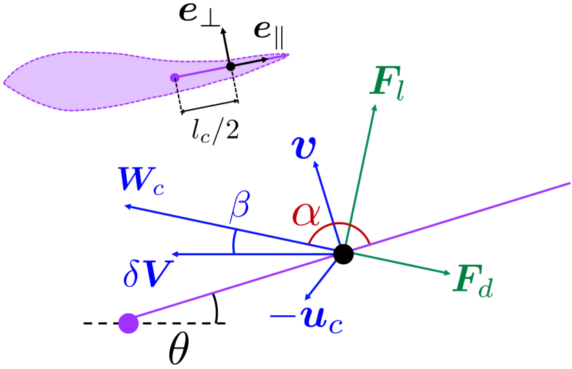
Figure 2: Schematic illustration of the flapping plate showing the relative velocity $\bm{W}_{c}$ and its relation to the drag and lift forces $\bm{F}_{d},~{}\bm{F}_{l}$.

The thrust forces $F_{d,i}$ and $F_{l,i}$ in Eq. (1) are the $X$-components of $\bm{F}_{d,i}$ and $\bm{F}_{l,i}$, and their sum reads

$$F_{d,i}+F_{l,i}=(\bm{F}_{d,i}+\bm{F}_{l,i})\cdot\bm{e}_{X}=\frac{\rho_{w}}{2}C_{F}(\alpha_{i},\beta_{i})H_{b}l_{c}W_{c,i}^{2},$$ (26)

$$C_{F}(\alpha_{i},\beta_{i})=C_{d}(\alpha_{i})\cos\beta_{i}+C_{l}(\alpha_{i})\sin\beta_{i}.$$ (27)

The hydrodynamic torque $\bm{N}_{d,i}+\bm{N}_{l,i}$ in Eq. (2) is given by

$$\bm{N}_{d,i}+\bm{N}_{l,i} = \frac{l_{c}}{2}\bm{e}_{\parallel,i}\times(\bm{F}_{d,i}+\bm{F}_{l,i})$$ (28)

$$= \frac{\rho_{w}}{4}C_{N}(\alpha_{i},\theta_{i}+\beta_{i})H_{b}l_{c}^{2}W_{c,i}^{2}\bm{e}_{Z},$$

$$C_{N}(\alpha_{i},\theta_{i}+\beta_{i}) = -C_{d}(\alpha_{i})\sin(\theta_{i}+\beta_{i})$$ (29)

$$\quad+C_{l}(\alpha_{i})\cos(\theta_{i}+\beta_{i}),$$

where $\bm{e}_{\parallel,i}=(\cos\theta_{i},\sin\theta_{i})$ is the unit vector parallel to the plate (see Fig. 2).

The third force in Eq. (1) is the Newton’s drag force acting on the swimmer’s body

$$F_{D,i}=-\mathrm{sgn}\left({{W_{b,i}}}\right)\rho_{w}C_{D}H_{b}L_{b}W_{b,i}^{2},$$ (30)

where $C_{D}$ is the drag coefficient, $\mathrm{sgn}\left({{\circ}}\right)$ is the sign function

$$\mathrm{sgn}\left({{x}}\right)=\left\{\begin{array}[]{ll}x/\absolutevalue{x}&[x\neq 0],\\ 0&[x=0],\end{array}\right.$$ (33)

and

$$W_{b,i}=\delta V_{i}-\bm{e}_{X}\cdot\bm{u}(X_{i},Y_{i},t)$$ (34)

is the relative velocity of the swimmer at the center of the body.

II.5 Inertial force and added mass

In the quasi-steady approximation, we add the inertial force as a non-steady term in the equation of motion Lighthill1960 . Since the inertial force is proportional to the acceleration, it is incorporated as an additional effective mass of the plate which is called the added mass Landau1987 . The added mass of an oscillating plate of finite aspect ratio is given by

$$m_{p}=\frac{\pi}{4}K\rho_{w}H_{b}^{2}l_{c},$$ (35)

where the numerical prefactor $K$ depends on the aspect ratio $H_{b}/l_{c}$ and is determined by fitting experimental data on airfoils Brennen1982 ; see Appendix B for details.

For the acceleration of the plate, we use the time-derivative of the velocity component that is perpendicular to the plate $(\bm{v}_{i}+\delta\bm{V}_{i})\cdot\bm{e}_{\perp,i}$. Then we obtain the inertial force as

$$\bm{F}_{m,i}=-m_{p}\derivative{(v_{i}-\delta V_{i}\sin\theta_{i})}{t}\bm{e}_{\perp,i},$$ (36)

which gives the thrust force $F_{m,i}$ in Eq. (1) as

$$F_{m,i}=\bm{F}_{m,i}\cdot\bm{e}_{X}=m_{p}\sin\theta_{i}\derivative{(v_{i}-\delta V_{i}\sin\theta_{i})}{t},$$ (37)

and the torque $\bm{N}_{m,i}$ in Eq. (2) as

$$\bm{N}_{m,i}=\frac{l_{c}}{2}\bm{e}_{\parallel,i}\times\bm{F}_{m,i}=-\frac{m_{p}}{2}l_{c}\derivative{(v_{i}-\delta V_{i}\sin\theta_{i})}{t}\bm{e}_{Z}.$$ (38)

II.6 Non-dimensionalization of equations

We reorganize the equations in a non-dimensional form. The unit of length is the body length $L_{b}$, the unit of time is taken as $\tau_{0}=1$ sec, and the unit mass unit is the body mass $M$. In the following, except for Appendix C, all quantities are non-dimensionalized by $L_{b}$, $\tau_{0}$, and $M$ unless otherwise stated, and expressed by the same symbols as before. (For example, we reexpress the dimensionless thrust speed $\delta V_{i}\tau_{0}/L_{b}$ by $\delta V_{i}$ and the bending stiffness $B\tau_{0}^{2}/ML_{b}^{3}$ by $B$.) In addition, we define the dimensionless constants

$$\chi_{h}=\frac{H_{b}}{L_{b}},\quad\chi_{c}=\frac{l_{c}}{L_{b}},\quad\chi_{\rho}=\frac{\rho_{w}}{\rho}.$$ (39)

Using the thrust forces (26), (30) and (37), and the torques (5), (6), (28) and (38), Eqs. (1) and (2) are rewritten as

$$\mathcal{M}_{i}\derivative{\delta V_{i}}{t}=\widehat{\mathcal{I}}_{i}\derivative{\omega_{i}}{t}+\mathcal{F}_{i},$$ (40)

$$\mathcal{I}\derivative{\omega_{i}}{t}=\widehat{\mathcal{M}}_{i}\derivative{\delta V_{i}}{t}+\mathcal{N}_{i},$$ (41)

respectively, where

$$\mathcal{M}_{i}=1+\frac{\pi}{4}\chi_{\rho}\chi_{c}\chi_{h}K\sin^{2}\theta_{i},~{}\mathcal{I}=1+\frac{3\pi}{16}\chi_{\rho}\chi_{h}K,~{}\widehat{\mathcal{M}}_{i}=\frac{3\pi}{8}\frac{\chi_{\rho}\chi_{h}}{\chi_{c}}K\sin\theta_{i},~{}\widehat{\mathcal{I}}_{i}=\frac{\pi}{8}\chi_{\rho}\chi_{c}^{2}\chi_{h}K\sin\theta_{i},$$ (42)

$$\mathcal{F}_{i}=\frac{1}{2}\chi_{\rho}\chi_{c}C_{F}(\alpha_{i},\beta_{i})W_{c,i}^{2}-\frac{\pi}{4}\chi_{\rho}\chi_{c}\chi_{h}K\omega_{i}\delta V_{i}\sin\theta_{i}\cos\theta_{i}-\mathrm{sgn}\left({{W_{b,i}}}\right)\chi_{\rho}C_{D}W_{b,i}^{2},$$ (43)

$$\mathcal{N}_{i}=\frac{3}{4}\frac{\chi_{\rho}}{\chi_{c}}C_{N}(\alpha_{i},\theta_{i}+\beta_{i})W_{c,i}^{2}+\frac{3\pi}{8}\frac{\chi_{\rho}\chi_{h}}{\chi_{c}}K\omega_{i}\delta V_{i}\cos\theta_{i}-3\frac{B}{\chi_{c}^{4}}\sin\theta_{i}+3\frac{N_{a,i}}{\chi_{c}^{3}}\sin(2\pi f_{a}t+\varphi_{i}).$$ (44)

We rewrite Eqs. (40) and (41) in the matrix form

$$\derivative{t}\matrixquantity[\delta V_{i}\\ \omega_{i}]=\frac{1}{\mathcal{M}_{i}\mathcal{I}-\widehat{\mathcal{M}}_{i}\widehat{\mathcal{I}}_{i}}\matrixquantity[\mathcal{I}&\widehat{\mathcal{I}}_{i}\\ \widehat{\mathcal{M}}_{i}&\mathcal{M}_{i}]\matrixquantity[\mathcal{F}_{i}\\ \mathcal{N}_{i}],$$ (45)

where

$$\mathcal{M}_{i}\mathcal{I}-\widehat{\mathcal{M}}_{i}\widehat{\mathcal{I}}_{i}=1+\frac{\pi}{4}\chi_{\rho}\chi_{h}K\left({\frac{3}{4}+\chi_{c}\sin^{2}\theta_{i}}\right)>0.$$ (46)

The stochastic differential equations (7) and (8) are rewritten as

$$\differential N_{a,i}=\frac{\differential t}{\tau_{a}}(\nu_{a}-N_{a,i})+\sqrt{2D_{a}}\differential w_{a,i},$$ (47)

$$\differential\varphi_{i}=\sqrt{2D_{\varphi}}\differential w_{\varphi,i},$$ (48)

where $\differential w_{a,i}$ and $\differential w_{\varphi,i}$ are the standard Wiener processes, and $D_{a}$ and $D_{\varphi}$ are the diffusion coefficients.

II.7 Numerical method

We numerically solve Eqs. (45), (47), and (48) with the vortex flow field (16). We integrate the equation of motion (45) by the Euler method with the time step $\Delta t=0.0005$. For the stochastic differential equations, we use It$\hat{\rm{o}}$ integral and replace the standard Wiener process by $\xi\sqrt{\Delta t}$, where $\xi$ is a random number generated by the standard Gauss distribution that is truncated at $\pm 5\sigma$ to prevent divergence of the solution. We also introduce a finite lifetime for the vortices to reduce computational cost. The vortex $n_{i}$ is deleted when it satisfies the condition $\exp(-(t-t_{n_{i}})/\tau_{\Gamma})\leq 10^{-3}$.

For the initial conditions, we used $\delta V_{i}=-U$, $\theta_{i}=0$, $\omega_{i}=0$, and $N_{a,i}=\nu_{a}$ for both fish1 ($i=1$) and fish2 ($i=2$), while $\varphi_{i}$ is chosen as a uniform random number in $[0,2\pi]$. Fish1 has the initial position $(X_{1},Y_{1})=(0,0)$, while for fish2, $X_{2}$ is chosen as a uniform random number in $[-d_{\parallel,\max},d_{\parallel,\max}]$ with $d_{\parallel,\max}=2.5$ and $Y_{2}=d_{\perp}$ (see Fig. 1(b)).

Each simulation runs up to $t_{\max}=80$. We obtain the amplitude $A_{i}(t)$ and the phase $\phi_{i}(t)$ of the flapping plate by Hilbert transformation of the tip position $y_{c,i}(t)$ in the time window $[t_{\max}-t_{H},t_{\max}]$ with $t_{H}=2^{17}\times\Delta t=65.536$ (see also Appendix A), and computed the frequency $f_{i}(t)=\{\phi_{i}(t)-\phi_{i}(t-\Delta t)\}/\Delta t$. We confirmed that a swimmer rapidly reaches steady swimming by $t=t_{\max}-t_{H}$ in the noiseless case. To avoid artifacts of the Hilbert transformation at both ends of the time interval, we introduce the cutoff $\delta t$ and use the interval $t\in[t_{\max}-t_{H}+\delta t,t_{\max}-\delta t]$ for time-averaging. We denote the time-average of the quantity $Q(t)$ by $\overline{Q}$.

In this model, the primary control parameters are $\{\chi_{c},~{}C_{\Gamma},~{}f_{a},~{}D_{a},~{}D_{\varphi},~{}d_{\perp}\}$, and $U$ and $\nu_{a}$ are varied depending on the case. We set the primary control parameters in accordance with experimental data; we summarize the parameters and their values used in the simulation in Appendix C.

III Solitary swimming

In this section, we show the results for solitary swimming. We omit the index $i$ as we consider only one fish.

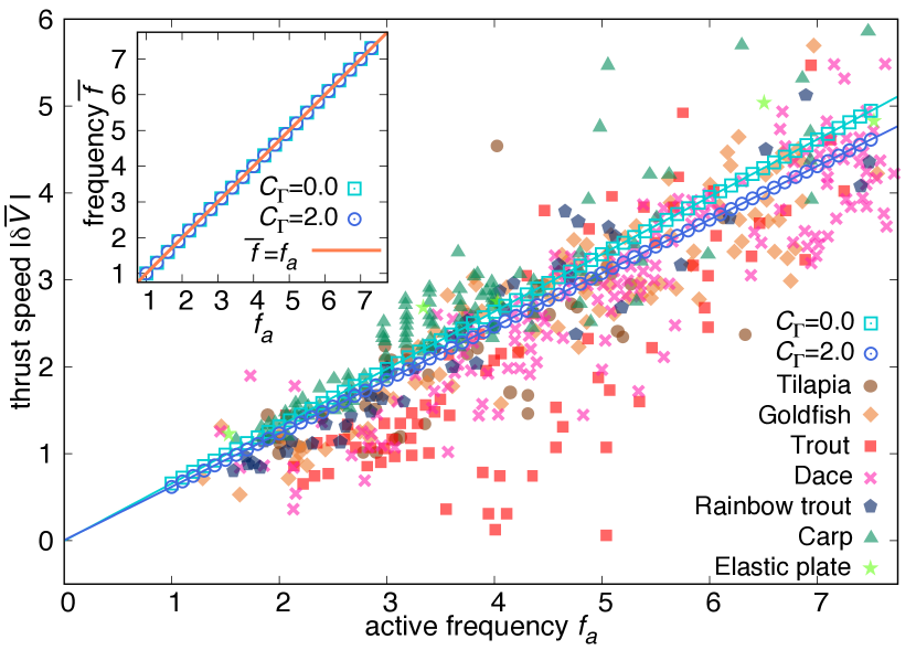
Figure 3: The thrust speed $\absolutevalue{\delta\overline{V}}$ as a function of the active frequency $f_{a}$. Open squares and open circles correspond to the case without vortices ($C_{\Gamma}=0.0$) and with vortices ($C_{\Gamma}=2.0$), respectively, and solid lines show the fitting by Eq. (49) (see also Table 2). The other types of points represent the experimental data for tilapia and carp Tanaka1996 , goldfish, trout, and dace Bainbridge1958 , rainbow trout Akanyeti2017 , and the data for the elastic plate model Gazzola2015 . In the inset, we show the time-averaged frequency $\overline{f}$ versus $f_{a}$, which is perfectly on the line $\overline{f}=f_{a}$.

III.1 The relation between thrust speed and tailbeat frequency

First we consider the noiseless case ($D_{a}=0,~{}D_{\varphi}=0$), for which the parameter set is $\{\chi_{c},~{}C_{\Gamma},~{}f_{a}\}$. We set $U=0$ by a Galilean transformation and without loss of generality, so that $V=\delta V$. For each parameter set $\{\chi_{c},~{}C_{\Gamma},~{}f_{a}\}$, we tune $\nu_{a}$ in increments of $\Delta\nu_{a}=0.01$ so that the time-averaged amplitude $\overline{A}$ becomes close to the prescribed value $A_{0}=0.1L_{b}$.

To test the validity of the model, we study the relation between the time-averaged thrust speed $\absolutevalue{\delta\overline{V}}$ and the active frequency $f_{a}=1.0$-7.5, with $\chi_{c}=0.375$ fixed.

As shown in Fig. 3, $\absolutevalue{\delta\overline{V}}$ increases linearly as a function of $f_{a}$, for the cases without vortices ($C_{\Gamma}=0.0$) and with vortices ($C_{\Gamma}=2.0$). The time-averaged tailbeat frequency $\overline{f}$ derived from Hilbert transformation is almost equal to the active frequency $f_{a}$ (see Fig. 3 inset). A linear relation between the thrust speed and tailbeat frequency was found in many experimental studies Bainbridge1958 ; Hunter1971 ; Webb1984 ; Akanyeti2017 ; Li2021 ; Nagai1979 ; Tanaka1996 . Our data are also nicely fitted by the linear relation

$$\absolutevalue{\delta\overline{V}}=\mu f_{a}+\mu^{\prime},$$ (49)

where $\mu$ and $\mu^{\prime}$ are constants. In Table 2, we show our results in comparison with the experimental data Tanaka1996 ; Nagai1979 ; Bainbridge1958 ; Akanyeti2017 and the numerical results for the elastic plate model Gazzola2015 . For both with and without vortices, the values of $\mu$ and $\mu^{\prime}$ fit in the range of the previous results. In particular, $\mu$ lies between 0.6 and 0.7 regardless of the presence of vortices, and is close to the experimental values. The intercept $\mu^{\prime}$ is almost zero (slightly negative). This is in agreement with the experimental results for five species, where $\mu^{\prime}=0$ is assumed Tanaka1996 ; Nagai1979 . On the other hand, two other experiments obtained negative values of $\mu^{\prime}$ Bainbridge1958 ; Akanyeti2017 . The origin of the negative intercept is unclear, but we may argue that the non-caudal fins (e.g. the pectoral fin) that rise from the body in low speed swimming Bainbridge1963 induce additional drag forces and dampen the thrust speed to zero at a finite tailbeat frequency.

Table 2: The coefficients $\mu$ and $\mu^{\prime}$ in Eq. (49). Our results are shown in the top two rows. The rest rows are results of experiments and other model. The data (T), (N), (B), and (A) are taken from the experiments in Ref. Tanaka1996 , Nagai1979 , Bainbridge1958 , and Akanyeti2017 , respectively, and (G) is from the elastic plate model Gazzola2015 .

	$\mu$	$\mu^{\prime}$
without vortices ($C_{\Gamma}=0.0$)	0.66	$-0.002$
with vortices ($C_{\Gamma}=2.0$)	0.61	$-0.004$
Tilapia (T)	0.576	0.0
Goldfish (N)	0.61	0.0
Goldfish (B)	0.64	$-0.20$
Trout (N)	0.62	0.0
Trout (B)	0.73	$-1.13$
Dace (N)	0.63	0.0
Dace (B)	0.74	$-1.02$
Rainbow trout (A)	0.67	$-0.16$
Carp (T)	0.695	0.0
Elastic plate (G)	0.72	$-0.12$

III.2 Other properties of noiseless swimming

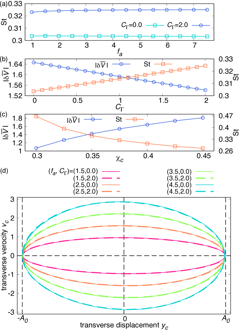
Figure 4: (a)-(c) The Strouhal number $\mathrm{St}$ and thrust speed $\absolutevalue{\delta\overline{V}}$ as functions of $f_{a}$, $C_{\Gamma}$, and $\chi_{c}$. (a) Square and circle points correspond to the case without vortices ($C_{\Gamma}=0.0$) and with vortices ($C_{\Gamma}=2.0$), respectively. We fixed $\chi_{c}=0.375$. (b)-(c) Circle points represent $\absolutevalue{\delta\overline{V}}$ and square points correspond to $\mathrm{St}$. In (b), we fixed $f_{a}=2.5$ and $\chi_{c}=0.375$; in (c), $f_{a}=2.5$ and $C_{\Gamma}=2.0$. (d) The trajectory of tailbeat in phase space ($y_{c},v_{c}$) for $\chi_{c}=0.375$. Solid and dashed lines correspond to the case without vortices ($C_{\Gamma}=0.0$) and with vortices ($C_{\Gamma}=2.0$), respectively. A larger $f_{a}$ gives a larger amplitude of the velocity.

Let us study some more properties of noiseless swimming. We introduce the Strouhal number

$$\mathrm{St}=\frac{2\overline{A}\,\overline{f}}{\absolutevalue{\delta\overline{V}}},$$ (50)

which characterizes the speed of flapping compared to the thrust. (The amplitude $\overline{A}$ is doubled following convention.) As shown in Fig. 4(a), the Strouhal number is given by $\mathrm{St}\gtrsim 0.3$ independent of $f_{a}$ and for $\chi_{c}=0.375$. This value is agreement with the experimental values of $\mathrm{St}\approx 0.2$-0.4, which are often close to $0.3$ for many species Gazzola2015 ; Gazzola2014 ; Triantafyllou1993 ; Taylor2003 .

Fig. 4(b) shows the dependence of $\absolutevalue{\delta\overline{V}}$ and $\mathrm{St}$ on the vortex strength $C_{\Gamma}$ with $f_{a}=2.5$ and $\chi_{c}=0.375$. The thrust speed $\absolutevalue{\delta\overline{V}}$ gradually decreases as $C_{\Gamma}$ increases, which is because the vortex flow increases the drag on the body and the plate. As a result, the Strouhal number increases according to the definition (Eq. (50)). In addition, we check the dependence of $\absolutevalue{\delta\overline{V}}$ and $\mathrm{St}$ on the relative fin length $\chi_{c}$; see Fig. 4(c). As the caudal part becomes longer, the thrust force and speed $\absolutevalue{\delta\overline{V}}$ increase nonlinearly due to the prefactor $K$ in the added mass (see Eq. (35) and Fig. 10(b)). The Strouhal number then decreases but stays in the experimentally observed range $\mathrm{St}\approx 0.2-0.4$ Gazzola2015 ; Gazzola2014 ; Triantafyllou1993 ; Taylor2003 , except for $\chi_{c}=0.3$.

Fig. 4(d) shows the tailbeat trajectory on the phase space $(y_{c},v_{c})$ where $v_{c}=\derivative*{y_{c}}{t}=l_{c}\omega\cos\theta$ is the transverse velocity. There is almost no difference between the trajectories in the case of $C_{\Gamma}=0.0$ and $C_{\Gamma}=2.0$. The trajectory is almost mirror symmetric with respect to the $y_{c}$-axis and $v_{c}$-axis. This symmetry of the caudal fin movement is observed for steady swimming of fish Bainbridge1963 . Furthermore, the peak value of $\absolutevalue{v_{c}}$ is good agreement with the experimental value: for example, the peak value is $\absolutevalue{v_{c}}\sim 1.5$-3.0 BL/s of dace with the swimming speed $\gtrsim 1.5$ BL/s Bainbridge1963 . It corresponds to the value for $f_{a}=2.5$-3.5 in Fig. 4(d) (see also Fig. 3 for the swimming speed in the range $f_{a}=2.5$-3.5).

III.3 The effect of physiological noises

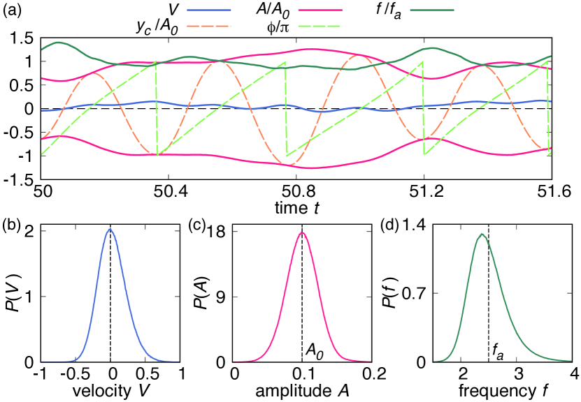
Figure 5: The effect of noise on swimming properties with $C_{\Gamma}=2.0,D_{a}=0.7,D_{\varphi}=0.25$. (a) Time evolution in the interval $4/f_{a}$. The solid line near the dashed line of zero is $V$ and The pair of solid lines are $A/A_{0}$ and $-A/A_{0}$. The upper solitary solid line is $f/f_{a}$. The sinusoidal dashed line is $y_{c}/A_{0}$ and the sawtooth-like dashed line is $\phi/\pi$. The normalized distribution $P$ of (b) the velocity $V$, (c) the amplitude $A$ with dashed line $A_{0}$, and (d) the frequency $f$ with dashed line $f_{a}$.

Here, we study the effect of physiological noises. To make the expected value of $V$ close to zero, we select the background flow speed $U=\absolutevalue{\delta V_{0}}$ where $\absolutevalue{\delta V_{0}}$ is the time averaged thrust speed $\absolutevalue{\delta\overline{V}}$ for the noiseless case. Hereafter, we fix $\chi_{c}=0.375$, which reproduces the thrust speed and active frequency, and $f_{a}=2.5$, which corresponds to the background flow speed $U\sim 1.5-1.6$ BL/s in the experiment Li2020 ; see Fig. 3.

Fig. 5(a) shows the typical time evolution of $V$ and normalized quantities $y_{c}/A_{0},~{}A/A_{0},~{}\phi/\pi,~{}f/f_{a}$ with noises. We define the probability distribution of any quantity $Q$ in each run as

$$p(Q)=\frac{1}{t_{H}-2\delta t}\int_{t_{\max}-t_{H}+\delta t}^{t_{\max}-\delta t}\differential t\,\delta(Q-Q(t)),$$ (51)

where $\delta(\circ)$ is Dirac delta function. Then we take the ensemble average of $p(Q)$ over 1000 independent runs to obtain the averaged probability distribution $P(Q)$. Shown in Fig. 5(b)-(d) are the distributions $P(V)$, $P(A)$, and $P(f)$ with the noise strengths $D_{a}=0.7$ and $D_{\varphi}=0.25$. For these values of $D_{a}$ and $D_{\varphi}$, the expected values of $A$ and $f$ are very close to the values $A_{0}$ and $f_{a}$ of the noiseless case, and justify the estimate of $\Gamma$ in Eq. (15). Furthermore, the noise strengths nicely reproduce the height, width, and asymmetry of the distributions observed for goldfish (Ref.Li2020 , Figs. 24 and 26 of the Supplementary Information). Therefore, we choose $D_{a}=0.7,~{}D_{\varphi}=0.25$ as the standard parameter values in the simulations. The dependence of the distributions on $D_{a}$ and $D_{\varphi}$ is shown in Appendix D.

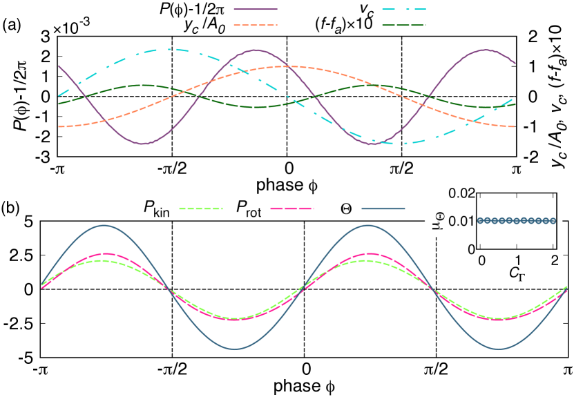
Figure 6: Profiles of various quantities characterizing the tailbeat as functions of the phase $\phi$, for $C_{\Gamma}=2.0$, $D_{a}=0.7$, and $D_{\varphi}=0.25$. (a) The phase distribution $P(\phi)$ subtracted by its period average, transverse displacement $y_{c}/A_{0}$, transverse velocity $v_{c}$, frequency shift $f-f_{a}$ versus $\phi$. (b) The power $P_{\mathrm{kin}}$ and $P_{\mathrm{rot}}$, and the energy dissipation rate $\Theta$ versus $\phi$. Inset: the dependence of $\mu_{\Theta}$ on $C_{\Gamma}$.

Next, we consider the profiles of various quantities that characterize the tailbeat. In Fig. 6(a), we show the average phase distribution $P(\phi)$. Its shift from the period average $1/(2\pi)$ slightly deviates from zero and oscillates with the period $\pi$. In addition, Fig. 6(a) shows the transverse displacement $y_{c}/A_{0}$, transverse velocity $v_{c}$, and frequency shift $f-f_{a}$ as functions of $\phi$: these quantities are time-averages over the interval $t\in[t_{\max}-\delta t,t_{\max}-t_{H}+\delta t]$ and $10^{4}$ simulations for each bin of $\phi$. We confirm that $y_{c}/A_{0}$ is proportional to $\cos\phi$ by definition of the Hilbert transformation (see Appendix A), and $v_{c}$ is proportional to $-\sin\phi$. Roughly speaking, the phase distribution $P(\phi)$ is large when the plate is swinging away from the midline of the body, and small when swinging back, but there is a phase delay. In other words, the frequency (phase velocity) $f$ is small when the plate is swinging away, and vice versa.

To elucidate the reason of non-uniformity of $P(\phi)$, we consider the energy dissipation rate $\Theta_{\mathrm{dis}}$, or the power required for swimming. It satisfies

$$\Theta_{\mathrm{dis}}=\derivative{E_{\mathrm{kin}}}{t}+\derivative{E_{\mathrm{rot}}}{t},$$ (52)

where $E_{\mathrm{kin}}=M(\delta V)^{2}/2$ is the translational kinetic energy of the body and $E_{\mathrm{rot}}=I_{c}\omega^{2}/2$ is the rotational kinetic energy of the plate. We divide the both sides of the equation by $ML_{b}^{2}/\tau_{0}^{3}$ and define the dimensionless energy dissipation rate $\Theta=\Theta_{\mathrm{dis}}\tau_{0}^{3}/ML_{b}^{2}$, which satisfies

$$\Theta=P_{\mathrm{kin}}+P_{\mathrm{rot}}\equiv\delta V\derivative{\delta V}{t}+\frac{\chi_{c}^{3}}{3}\omega\derivative{\omega}{t}.$$ (53)

Note that $\Theta>0$ corresponds to the situation that a swimmer consumes the swimming energy. Fig. 6(b) shows that $\Theta$, $P_{\mathrm{kin}}$, and $P_{\mathrm{rot}}$ oscillate with the period $\pi$ as a function of $\phi$. We find that the energy dissipation rate tends to be positive when $P(\phi)-1/2\pi<0$ (and $f-f_{a}>0$), although there is a phase delay. This result indicates that the swimmer consumes energy in quick motion of the caudal plate when it is swinging back to the midline, and gain energy from the flow when the plate is swinging away. The cycle-average of the energy dissipation rate, defined by $\mu_{\Theta}=\int_{-\pi}^{\pi}d\phi\Theta(\phi)P(\phi)$, is confirmed to be positive, but is very small compared to the amplitude of $\Theta$, as shown in the inset of Fig. 6(b). We also find that $\mu_{\Theta}$ is almost independent of the vortex strength $C_{\Gamma}$.

IV Pair swimming

In this section, we show the results for a pair of swimmers (labeled by $i=1,2$). We fix $\chi_{c}=0.375$, $f_{a}=2.5$, $D_{a}=0.7$, and $D_{\varphi}=0.25$, and choose the vortex strength $C_{\Gamma}$ and the transverse distance between the swimmers $d_{\perp}$ as tunable control parameters. We confirmed that our results do not change if fish 2 is positioned to the left of fish1, as expected from the left-right symmetry of the model (data not shown).

IV.1 Correllation between the phase difference and distance

First, we consider the phase difference between the phases of the tailbeat of the leader and follower, defined by

$$\psi=\left\{\begin{array}[]{ll}\phi_{1}-\phi_{2}&[X_{1}<X_{2}],\\ \phi_{2}-\phi_{1}&[X_{2}<X_{1}].\end{array}\right.$$ (56)

To see the correlation between the phase difference and the longitudinal distance $d_{\parallel}=\absolutevalue{X_{1}-X_{2}}$, we introduce the conditional probability distribution $P(\psi;d_{\parallel})$. As a function of $\psi$, it is normalized in each bin of $d_{\parallel}$ by the condition $\int_{-\pi}^{\pi}\differential\psi P(\psi;d_{\parallel})=1$. Note that $d_{\parallel}$ and $\psi$ change with time in a simulation.

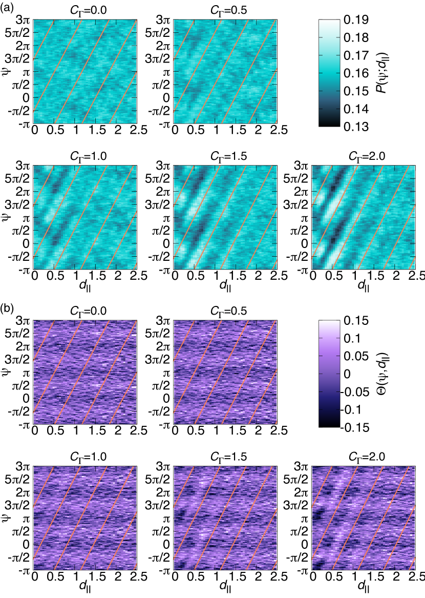
Figure 7: Dependence of (a) the probability distribution $P(\psi;d_{\parallel})$ and (b) the dissipation rate $\Theta(\psi,d_{\parallel})$ on $C_{\Gamma}$ with $d_{\perp}=0.2$. Note that plots in the range $\psi\in[-\pi,\pi]$ is periodically extended to $\psi\in[\pi,3\pi]$ for visibility. The solid lines represent Eq. (57) with $\psi_{0}$ shifted by integer multiples of $2\pi$.

In Fig. 7(a), we show $P(\psi;d_{\parallel})$ for several values of $C_{\Gamma}$ with $d_{\perp}=0.2$ fixed. For the case without vortices ($C_{\Gamma}=0$), the distribution $P(\psi;d_{\parallel})$ is almost uniform and close to the average value $1/(2\pi)\simeq 0.159$. Correlation between $\psi$ and $d_{\parallel}$ emerges with increasing $C_{\Gamma}$, and a periodic pattern is clearly observed for $C_{\Gamma}=2.0$. The correlation is strong for the distance $d_{\parallel}\lesssim 1$, and is detectable up to $d_{\parallel}\sim 2$. This result is qualitatively the same as the experiment on goldfish Li2020 (see Fig. 18 of Supplementary Information of the reference).

Theoretically, synchronization of the tailbeat is achieved at the phase difference

$$\psi=\frac{2\pi f_{a}}{U}d_{\parallel}+\psi_{0},\quad\psi_{0}=-\frac{\pi f_{a}\chi_{c}}{U}.$$ (57)

Here, $d_{\parallel}/U$ gives the time for the vortex emitted by the leader to travel the distance $d_{\parallel}$, and $2\pi f_{a}d_{\parallel}/U$ is the increment of phase of the leader in this time interval Li2020 . We formulate the phase shift $\psi_{0}$ using the fact that the vortex emitted from the tip of the leader’s plate affects the follower most strongly at the mid-point of the follower’s plate (see the definitions of the drag force $\bm{F}_{d}$ and the lift force $\bm{F}_{l}$ in Eqs. (23) and (24)). This means that the interaction between the two swimmers is strongest and their motion is synchronized at the distance $d_{\parallel}=\chi_{c}/2$, which gives $\psi_{0}=-(2\pi f_{a}/U)\times(\chi_{c}/2)$. As shown in Fig. 7(a), the formula (57) reproduces the peak lines of $P(\psi;d_{\parallel})$ fairly well. The phase shift $\psi_{0}$ is varied by the background flow speed $U$ (=$\absolutevalue{\delta V_{0}}$), which is a function of $C_{\Gamma}$, and the range is $\psi_{0}=-\pi\times 0.57$-0.61. The dependence of $P(\psi;d_{\parallel})$ on $d_{\perp}$ is shown in Appendix E.

IV.2 Spontaneous reduction of energy consumption

Finally, we study the energy dissipation rate as a function of the phase difference $\psi$ and the front-back distance $d_{\parallel}$. We traced the swimmer 1 for each run and take the ensemble average over $10^{4}$ runs to define the energy dissipation rate $\Theta(\psi,d_{\parallel})$. Note that this is equivalent to taking the average of the leader and follower in a single run over a very long time.

The result is shown in Fig. 7(b). With increasing $C_{\Gamma}$, $\Theta(\psi,d_{\parallel})$ develops an oblique stripe that is parallel to the theoretical line (Eq. (57)) in the range $d_{\parallel}\lesssim 1$. This result is consistent with the experimental results on robotic fish Li2020 . Also, the energy dissipation rate shows a periodic dependence on $\psi$ with the period $\pi$, which is independent of $d_{\parallel}$ and even without the vortex-mediated interaction ($C_{\Gamma}=0$). This dependence is explained by the periodicity of the energy dissipation rate $\Theta(\phi)$ for a solo swimmer shown in Fig. 6(b); see Appendix E for a detailed discussion.

The expected value of the energy dissipation rate is defined by

$$\langle\Theta(d_{\parallel})\rangle=\int_{-\pi}^{\pi}\differential\psi P(\psi;d_{\parallel})\Theta(\psi,d_{\parallel}).$$ (58)

We obtain $\langle\Theta(d_{\parallel})\rangle$ using 50 sets of $10^{4}$ simulations to calculate the average and standard deviation. Fig. 8(a) shows the dependence of the averaged $\langle\Theta(d_{\parallel})\rangle$ on $C_{\Gamma}$. For $C_{\Gamma}=0$, $\langle\Theta(d_{\parallel})\rangle$ is independent of $d_{\parallel}$ and reproduces the value $\mu_{\Theta}\simeq 0.01$ for solitary swimming, as it should (see also Appendix E). On the other hand, for $C_{\Gamma}>0$, $\Theta$ shows a complex distance dependence. It makes a minimum in the interval $0<d_{\parallel}<\chi_{c}/2$, and even turns negative for $C_{\Gamma}=1.5$ and $2.0$. The negative dissipation means that the swimmer gains energy from the flow in one cycle of tailbeat. In $\chi_{c}/2<d_{\parallel}<0.5$, $\langle\Theta(d_{\parallel})\rangle$ shows a gradual increase and crosses $\mu_{\Theta}$. It makes a sharp peak at $d_{\parallel}\sim 0.6$, and converges to $\mu_{\Theta}$ in $d_{\parallel}\gtrsim 1$ where the distribution $P(\psi;d_{\parallel})$ becomes uniform. We show the dependence of the energy dissipation rate on $d_{\perp}$ in Appendix E.

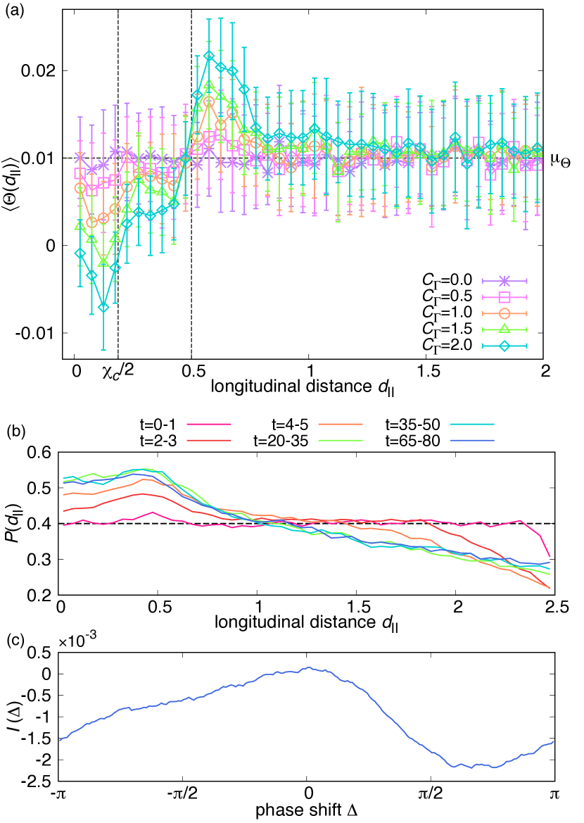
Figure 8: (a) The expected value of the dissipation rate $\langle\Theta\rangle$ as a function of the longitudinal distance $d_{\parallel}$. The vortex strength $C_{\Gamma}$ is varied in $[0,2.0]$. The error bar is the standard deviation of 50 sets of simulations. The horizontal dashed line represents the expected value of the dissipation rate $\mu_{\Theta}$ for solitary swimming. The vertical dashed lines correspond to a half of the plate length ($\chi_{c}/2$) and a half of the body length. (b) Probability distribution of the longitudinal distance in different time intervals, normalized in the range $0<d_{\parallel}<2.5$. It develops deviations from the initial uniform distribution (horizontal dashed line) and reaches a steady distribution with a peak in the range $d_{\parallel}<0.5$. (c) The overlap integral between the probability distribution $P(\psi;d_{\parallel})$ and the energy dissipation rate $\Theta(\psi,d_{\parallel})$ as a function of the phase shift $\Delta$ (see text for the definition). The transverse distance is fixed to $d_{\perp}=0.2$ in all the plots and $C_{\Gamma}=2.0$ in (b) and (c).

In Fig. 8(b), we plot the distribution of the longitudinal distance, which is computed in different time intervals and is normalized in the range $0<d_{\parallel}<2.5$. It rapidly develops deviations from the initial uniform distribution and reaches a steady distribution by $t=20$. The steady distribution has a broad peak in the region $d_{\parallel}<0.5$, which corresponds to the region where the energy dissipation rate is reduced (see Fig. 8(a)). The distribution decreases with the distance for $d_{\parallel}>0.5$.

While we showed that the energy dissipation rate is reduced by vortex phase matching, its minimum is shifted from the most probable phase difference given by Eq.(57), as shown in Fig. 7(b). In order to quantify the shift, we define the overlap between the probability distribution $P(\psi;d_{\parallel})$ and the energy dissipation rate $\Theta(\psi,d_{\parallel})$ by

$$I(\Delta)=\int_{-\pi}^{\pi}\differential\psi P(\psi;d_{\parallel})\Theta(\psi-\Delta,d_{\parallel}).$$ (59)

Here, we introduced the phase shift $\Delta$ to find the difference between the the energetically optimal value of $\psi$ and the most probable value of $\psi$. If $I(\Delta)$ is minimized at $\Delta=\Delta_{0}$, the former is given by

$$\psi_{E}=\frac{2\pi f_{a}}{U}d_{\parallel}+\psi_{0}-\Delta_{0},$$ (60)

instead of Eq.(57) for the latter. In Fig. 8(c), we plot the overlap integral averaged over the distace $0<d_{\parallel}<0.5$. Note that $I(0)$ gives the energy dissipation rate in Fig. 8(c) averaged over the same distance range. We find that $I(\Delta)$ is maximal around $\Delta=0$ and minimal in the range $\Delta(=\Delta_{0})\simeq\pi\times 0.6$-$0.7$. It indicates that the actual distribution of the phase difference does not minimize the energy dissipation rate.

V Conclusions

We constructed a new self-propelled model that reproduces many experimental features of carangiform and subcarangiform swimming. For the hydrodynamic part, we adopted the quasi-steady approximation Nagai1996 ; Hirayama2000 and introduced the Rankine vortex street which was not considered in the previous self-propelled models Tchieu2012 ; Gazzola2016 ; Filella2018 ; Deng2021 ; Gazzola2015 . By incorporating the physiological noises, we modeled time evolution of the phase of tailbeat and the distance of swimmers, which allowed the model fish to spontaneously select the swimming pattern. This is regarded as a significant advance from the previous models that fix the phase of tailbeat (and the relative distance) Hemelrijk2015 ; Daghooghi2015 ; Maertens2017 ; Li2019 ; Zhu2014 ; Park2018 ; Peng2018 ; Dewey2014 ; Boschitsch2014 ; Becker2015 ; Newbolt2019 ; Oza2019 . For body kinematics, our model with a single flapping plate is simpler than the two plates model Nagai1996 ; Hirayama2000 and the elastic plate models Taylor1952 ; Gazzola2015 , and has the merit to reduce computational cost. Now let us discuss the type of fish and swimming mode for which our model can be applied. As we take the body length as the unit of length, our model can be applied to a (sub)carangiform swimmer with any body length, 30 to 50 percents of which exhibits undulating motion. We choose the hydrodynamic parameters so that ${\mathrm{Re}}\sim\mathcal{O}(10^{5})$, which corresponds to the steady swimming of a typical (sub)carangiform swimmer (see also Appendix C for the choice of parameters). In the steady swimming, the swimming speed 1-5 BL/s is maintained for more than 1 hour. On the other hand, our model cannot be applied to a swimming speed $\gtrsim 5$ BL/s, which corresponds to the fast-start with the duration $\sim 0.1$ sec and ${\mathrm{Re}}\gtrsim\mathcal{O}(10^{6})$ Domenici1997 . In addition, we do not consider burst-and-coast swimming which has a cycle with active phase and gliding phase instead of the continuous fin motion GLi2021 . The burst-and-coast swimming is typically adopted by small fish and gives ${\mathrm{Re}}\lesssim\mathcal{O}(10^{4})$.

For solo swimming, the model reproduces the linear relation between the frequency of tailbeat and the thrust speed established for many species of fish Tanaka1996 ; Nagai1979 ; Bainbridge1958 ; Akanyeti2017 (Fig. 3). Self-induced vortices have only a minor effect on the thrust speed, as found with the elastic plate model Gazzola2015 . The elastic plate model also reproduced the frequency-speed relation, but by assuming the amplitude of tailbeat an order of magnitude smaller than the typical experimental value $A_{0}=0.1L_{b}$. It implies that the elastic plate swimmer has much higher swimming efficiency than real fish. We used the standard amplitude $A_{0}/L_{b}=0.1$ and the plate length $\chi_{c}=0.375$ to reproduce the relation. In addition, our model reproduces the typical Strouhal number $\mathrm{St}\approx 0.3$ Gazzola2014 ; Triantafyllou1993 ; Taylor2003 (see Fig. 4(a)-(c)), and the trajectory of tailbeat agrees with that of dace in steady swimming Bainbridge1963 (see Fig. 4(d)).

The two noise amplitudes ($D_{a},D_{\varphi}$) enabled us to fine-tune the probability distributions of the thrust speed and the amplitude and frequency of the tailbeat. We chose $D_{a}=0.7$ and $D_{\varphi}=0.25$ by matching the distribution functions with those of goldfish Li2020 (see Fig. 5(b)-(d) and Appendix D). Note that the physiological noises affect the motion of the caudal muscles, and therefore enter the equations of motion only via the torque. We neglected the effect of hydrodynamic turbulence, which could be introduced in the model as noises in both the thrust force and torque. The physiological and hydrodynamic noises may have different roles in modifying the swimming pattern, but they are beyond the scope of the present study.

For a pair of swimmers, we showed statistically that they adjust the phase difference depending on the front-back distance. The probability distribution of the phase difference $\psi$ shows a strong anisotropy in the short distance $d_{\parallel}\lesssim 1$ (see Fig. 7(a)) which is qualitatively consistent with the result on goldfish Li2020 . The correlation between $\psi$ and $d_{\parallel}$ is described by the theoretical relation (57), where we explicitly derived the formula for the phase shift $\psi_{0}$. The formula is generalized as $\psi_{0}=-2\pi f_{a}d_{0}/U$, where $d_{0}$ is the distance between the plate tip and the point on the plate P where the flow has the strongest effect on the flapping motion. We numerically obtained $\psi_{0}\approx-0.6\pi$, while the experiment on goldfish shows $\psi_{0}\approx-0.2\pi$. The difference between the two results could be explained as follows. In our model, P is the mid-point of the plate ($d_{0}=l_{c}/2$). On the other hand, the experimental value of $\psi_{0}$ implies that the point P is closer to the tip of the fin than in our model. This seems to be consistent with fact that the stiffness of the caudal part decreases as we go from the peduncle to the tip of the fin McHenry1995 , and thus the fin is easier to be deformed than the peduncle.

The energy dissipation rate $\Theta(\psi,d_{\parallel})$ also has a pattern described by the linear relation between $\psi$ and $d_{\parallel}$ in $d_{\parallel}\lesssim 1$ (see Fig. 7(b)). However, the phase difference $\psi_{E}$ that minimizes $\Theta(\psi,d_{\parallel})$ is shifted from the most probable phase difference by $-\Delta_{0}$. The value of $\psi_{E}$ at $d_{\parallel}=0$ is given by $\psi_{E0}=\psi_{0}-\Delta_{0}$, and the numerically obtained values $\psi_{0}\approx-0.6\pi$ and $\Delta_{0}\approx\pi\times 0.6-0.7$ give $\psi_{E0}\approx\pi\times 0.7-0.8$ (mod $2\pi$). A shift between the energetically optimal and the most probable phase differences is also found in the experiment Li2020 . There, the power efficiency of a robotic fish is fitted by the same formula with $\psi_{E0}\approx 0.3\pi$ Li2020 , and is larger than $\psi_{0}$ for the distribution of goldfish by $0.5\pi$. The origin of the difference between our and experimental values of $\psi_{E0}$ is unclear, but we should note that the probability distribution for robotic fish may differ from that of goldfish, and it could explain the difference. More importantly, the nonzero value of $\Delta_{0}$ means that the realized phase difference is not the one that minimizes the energy dissipation rate. This is in line with the observation that hydrodynamic synchronization does not always minimize energy dissipation rate Elfring2009 ; Liao2021 , and supports the importance to model the phase dynamics.

The experiment Li2020 also showed that the change in the power efficiency is small in the range of the transverse distance of 0.27-0.33 body length, which is also reproduced by our model (see $d_{\perp}=0.25$-0.3 in Fig. 12(b)). On the other hand, the horizontal stripe pattern in Fig. 7(b) is explained analytically by the distributions for a solo swimmer; see Appendix E. This pattern is not found in the experimental result on robotic fish, possibly due to the short measurement range of the longitudinal distance and large fluctuations Li2020 .

The expected energy dissipation rate $\langle\Theta(d_{\parallel})\rangle$ shows that the spontaneous reduction of energy consumption for the distance $d_{\parallel}\lesssim 0.5$, which roughly corresponds to the region of the strongest hydrodynamic interactions for a pair of goldfish Li2020 . At a larger distance, the energy dissipation rate becomes larger than that of solo swimming. These results are qualitatively consistent with those for robotic fish Li2020 : In Fig. 10 of Supplementary Information of the paper, it is shown that the efficiency of the electric power increases when the longitudinal distance is less than 0.7 body lengths, and can adopt negative value at the distance $\sim 0.8$ body lengths. Furthermore, we found that the distribution of the longitudinal distance develops a peak in the region $d_{\parallel}<0.5$ in the course of time. It means that the energetically favorable distance is dynamically selected by the swimmers.

Finally, there are some aspects to be addressed in the future. Our model can be applied to carangiform and subcarangiform swimmers, but not to the other types of fish Sfakiotakis1999 ; Lauder2005 . To reproduce the anguilliform, which is an undulating motion of the large part of the body, we need to introduce more hinges such as in the elastic plate model Gazzola2015 . The shape of the caudal fin is also an important factor to determine the swimming characteristics Hirayama2000 . The rectangular plate in our model is suited to many of carangiform and subcarangiform swimmers Bainbridge1963 , while tuna, representing the thunniform, has a thin crescent-shaped caudal fin. The thrust speed we obtained for $\chi_{c}=0.3$ is smaller than the measurement for yellowfin tuna (Thunnus albacares) Shadwick2008 (see also Fig. 4(c)), which is possibly due to the difference in the fin shapes.

The Rankine vortex street gives a fair representation of the vortex flow at low computational cost, but the flow field around real fish is more complex. For example, we may incorporate the dipolar flow field Filella2018 and collision process between the vortex and the swimmers Hemelrijk2015 . Turbulent flow at a small scale might be treated as noises on the thrust force and torque, although their mode structures are highly nontrivial. Our single-hinge model is a minimal model of locomotion gait, and does not capture the motion of the anterior part of the body. Although the head-beat amplitude is typically an order of magnitude smaller than the tailbeat amplitude Santo2021 , it can generate a sizable thrust force in the anterior part Wen2013 ; Lucas2020 . This thrust force affects hydrodynamic interaction in in-line configurations Thandiackal2023 . The present work focuses on vortex phase matching at transversal distance $d_{\perp}\gtrsim 0.2$ and $d_{\parallel}\lesssim 1$, and the analysis of vortex-mediated interaction in in-line configurations with $d_{\perp}\sim 0$ and $d_{\parallel}\gtrsim 1$ is left for future work. Our model is also limited to one-dimensional motion mimicking the experiment with background flow (for example, in the experiment with two gold fish Li2020 , they move in the lateral direction only in the range 0.27-0.33 BL). In order to extend it to two- or three-dimensional motion, we would need to integrate it with phenomenological self-propelled particle models with repulsion, attraction, and alignment interactions, which are presumably topological Gautrais2012 ; Calovi2014 ; Filella2018 ; Ito2022a ; Ito2022b , and also the three-dimensional flow field of a vortex ring Nauen2002 . Inclusion of these aspects will be an interesting issue for the future.

Author Contributions

Susumu Ito: Conceptualization (lead); Investigation (lead); Validation (lead); Visualization (lead); Writing - original draft (lead); Writing - review & editing (equal). Nariya Uchida: Conceptualization (supporting); Supervision (lead); Writing - review & editing (equal).

Appendix A Hilbert transformation

Figure 9: Time evolution of the acceleration $\derivative*{V}{t}$ and the velocity $V$ of a swimmer from the initial state to the end of a simulation ($t=80$) with $\chi_{c}=0.375,~{}f_{a}=2.5,~{}C_{\Gamma}=2.0,~{}D_{a}=0.7$, and $D_{\varphi}=0.25$. The Hilbert transform is conducted in the time window with the duration $t_{H}$. The left top inset represents the time evolution for $t\in[0,1.2]$, and the right top inset represents the time evolution for $t\in[70,71.2]$.

The Hilbert transformation is a mathematical method to extract the amplitude and the phase from oscillating time series data Huang2014 . We define the Hilbert transform $\hat{y}_{c}(t)$ of the plate tip motion $y_{c}(t)$ by the principal value integral

$$\hat{y}_{c}(t)=\frac{1}{\pi}\mathcal{P}\int_{-\infty}^{\infty}\differential t^{\prime}\frac{y_{c}(t^{\prime})}{t-t^{\prime}}.$$ (61)

Using the Fourier representation

$$y_{c}(t)=\frac{1}{2\pi}\int_{-\infty}^{\infty}\differential\omega\,y_{c,\omega}e^{i\omega t}$$ (62)

and residue theorem of complex integtation, the integral (61) becomes

$$\hat{y}_{c}(t)=\frac{1}{2\pi}\int_{-\infty}^{\infty}\differential\omega\,y_{c,\omega}\mathrm{sgn}\left({{\omega}}\right)e^{i\left({\omega t-\frac{\pi}{2}}\right)},$$ (63)

where $\mathrm{sgn}\left({{\circ}}\right)$ is the sign function (see Eq. (33)). For example, for constants $a$, $\omega$, and $\phi_{0}$, $y_{c}(t)=a\cos(\omega t+\phi_{0})$ and $y_{c}(t)=a\sin(\absolutevalue{\omega}t+\phi_{0})$ is transformed to $\hat{y}_{c}(t)=a\sin(\absolutevalue{\omega}t+\phi_{0})$ and $\hat{y}_{c}(t)=a\cos(\omega t+\phi_{0})$, respectively. Based on the formula (63), we can define the amplitude

$$A(t)=\sqrt{y_{c}^{2}(t)+\hat{y}_{c}^{2}(t)}$$ (64)

and the phase

$$\phi(t)=\tan[-1](\frac{\hat{y}_{c}(t)}{y_{c}(t)}).$$ (65)

This definition indicates $y_{c}(t)=A(t)\cos\phi(t)$.

Fig. 9 shows time evolution of the acceleration $\derivative*{V}{t}$ and the velocity $V$ of a swimmer. As indicated in the left top inset, the acceleration establishes a steady oscillatory pattern in a short time $t\sim{\cal O}(1)$, and we conducted the Hilbert transformation for the steady swimming.

Appendix B Drag and lift coefficient $C_{d},~{}C_{l}$ and coefficient $K$ of added mass

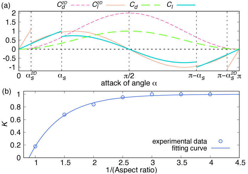
Figure 10: Plots of the hydrodynamic coefficients. (a) Dependences of $C_{d}$ (thick dashed line) and $C_{l}$ (thick solid line) on the angle of attack $\alpha$. The parameters are $c_{d}=1.0,~{}c_{l0}=1.0,~{}c_{l}=0.7,~{}\alpha_{s}=35^{\circ}$. $C_{d}^{2D}$ (thin dashed line) and $C_{l}^{2D}$ (thin solid line) are coefficients for a two dimensional plate aerofoil ($\alpha_{s}^{2D}=10^{\circ}$). (b) The added mass prefactor $K$ as a function of the inverse aspect ratio. The points show the experimental data Brennen1982 . The solid line fits the data by Eq. (77) with $a_{K}=1.82,~{}b_{K}=0.89$.

The drag coefficient $C_{d}(\alpha)$ and the lift coefficient $C_{l}(\alpha)$ of a plate with a finite aspect ratio in Eqs. (23) and (24) are derived by modifying the formula for a two-dimensional plate Ortiz2015 . The two-dimensional plate has the drag coefficient

$$C_{d}^{2D}(\alpha)=2\sin^{2}\alpha,$$ (66)

and the lift coefficient

$$C_{l}^{2D}(\alpha)=\left\{\begin{array}[]{ll}2\pi\sin\alpha&[\alpha<\alpha_{s}^{2D}],\\ \sin 2\alpha&[\alpha_{s}^{2D}<\alpha<\pi-\alpha_{s}^{2D}],\\ -2\pi\sin\alpha&[\alpha>\pi-\alpha_{s}^{2D}],\end{array}\right.$$ (70)

where $\alpha_{s}^{2D}\sim 10^{\circ}$ is a stall angle due to separation of flow at the rear of the airfoil (see Fig. 10(a)) Jiang2014 . These coefficients are symmetric about $\alpha=\pi/2$. For a plate of finite aspect ratio, $C_{d}(\alpha)$ and $C_{l}(\alpha)$ become smaller than $C_{d}^{2D}(\alpha)$ and $C_{l}^{2D}(\alpha)$, respectively, and a stall angle $\alpha_{s}$ is larger than $\alpha_{s}^{2D}$ Ortiz2015 , because the pressure is dispersed in the transverse direction and prevents flow separation. Referring to the data in Ref. Ortiz2015 , we formulate the drag coefficient as

$$C_{d}(\alpha)=c_{d}\sin^{2}\alpha,$$ (71)

and the lift coefficient as

$$C_{l}(\alpha)=\left\{\begin{array}[]{ll}c_{l0}\frac{\sin\alpha}{\sin\alpha_{s}}&[\alpha<\alpha_{s}],\\ c_{l}\frac{\sin 2\alpha}{\sin 2\alpha_{s}}&[\alpha_{s}<\alpha<\pi-\alpha_{s}],\\ -c_{l0}\frac{\sin\alpha}{\sin\alpha_{s}}&[\alpha>\pi-\alpha_{s}].\end{array}\right.$$ (75)

(see Table 3 for the values of $c_{d},~{}c_{l0},~{}c_{l},~{}\alpha_{s}$). They are plotted and compared with the two-dimensional case in Fig. 10(a).

Next, we consider the added mass of a plate in Eq. (35). An added mass per unit length of an oscillating two-dimensional plate with height $H_{b}$ in a potential flow is theoretically given by Wendel1956

$$m_{p}^{2D}=\frac{\pi}{4}\rho_{w}H_{b}^{2}.$$ (76)

For a plate with a finite aspect ratio ($H_{b}/l_{c}\lesssim 1$) in Eq. (35), we have the additional factor $K(\leq 1)$ that depends on the inverse aspect ratio $x=l_{c}/H_{b}$. The behavior of $K(x)$ is determined using the experimental results Brennen1982 , and $K\rightarrow 1$ in the low aspect ratio limit; see Fig. 10(b). Because $K$ rapidly approaches 1 as $x\to\infty$, we assumed the exponential function

$$K(x)=1-e^{-a_{K}(x-b_{K})}$$ (77)

and determined the constants $a_{K}$ and $b_{K}$ by fitting to the experimental data.

Appendix C Parameters

Table 3: List of the parameters. We rescaled the parameter values by the body length $L_{b}$, timescale $\tau_{0}=1$sec, and body mass $M$. (BL means the body length.)

symbol	meaning	experiment	simulation (rescaled)
$H_{b}$	body height	$\sim 0.3$ BL Jones1999	–
$l_{c}$	length of the caudal part	$\sim 0.3$-0.5 BL Lauder2005 ; Sfakiotakis1999	–
$\chi_{h}$	$H_{b}/L_{b}$	–	0.3
$\chi_{c}$	$l_{c}/L_{b}$	–	0.3-0.45
$A_{0}$	amplitude of tailbeat	$\sim 0.1$ BL Bainbridge1958 ; Hunter1971 ; Webb1984 ; Akanyeti2017 ; Li2021	0.1
$\rho$	effective density of the body	$\sim 41$ kg m-3 Jones1999	–
$\rho_{w}$	density of water	$\sim 1000$ kg m-3	–
$\chi_{\rho}$	$\rho_{w}/\rho$	–	25
$C_{D}$	drag coefficient of the body	$\sim 0.02$-0.07 Tandler2019	0.037 Ilio2018
$c_{d}$	drag coefficient of the plate	$\sim 1.0$ Ortiz2015	1.0
$c_{l0}$	lift coefficient of the plate (before stall)	$\sim 1.0$ Ortiz2015	1.0
$c_{l}$	lift coefficient of plate the (after stall)	$\sim 0.7$ Ortiz2015	0.7
$\alpha_{s}$	stall angle	$\sim 35^{\circ}$ Ortiz2015	35∘
$r_{R}$	radius of a vortex core	$\sim 0.04$-0.05 BL Nauen2002 ; Akanyeti2017	0.04
$\Gamma$	circulation of a vortex	$\sim 0.06$-0.25 BL2 s-1 Nauen2002 ; Wise2018	–
$C_{\Gamma}$	prefactor of the circulation	$\gtrsim 1.0$ Schnipper2009 ; Agre2016	0.0-2.0
$\tau_{\Gamma}$	decay time of a vortex	$\sim 2.0$ s Oza2019	2.0
$B$	bending stiffness	$\sim 10^{-4}$ N m2 McHenry1995	1.0
$f_{a}$	active frequency	–	1.0-7.5
$\tau_{a}$	damping timescale of $N_{a}$	–	1.0
$D_{a}$	diffusion coefficient for $N_{a}$	–	0-1.0
$D_{\phi}$	diffusion coefficient for $\varphi$	–	0-1.0
$d_{\perp}$	transverse distance	0.27-0.33 BL Li2020	0.2-0.4

Here, we define the parameters in our model by comparison to experimental values. See Table 3 for summary of the parameters.

We use the body height $H_{b}=0.3$ BL (body length) which is the averaged value of many species of fish Jones1999 , and the length of caudal part $l_{c}=0.3$-0.45 BL for carangiform and subcarangiform Lauder2005 ; Sfakiotakis1999 . The effective density of body $\rho$ is 41 kg m^-3 is obtained by averaging over various species of fish Jones1999 , and thus we use $\chi_{\rho}=\rho_{w}/\rho=25$. The amplitude of the tailbeat $A_{0}=0.1$ BL is ubiquitous for many species of fish at various swimming speeds Bainbridge1958 ; Hunter1971 ; Webb1984 ; Akanyeti2017 ; Li2021 ; NoteA0 .

In our system, the speed of background flow is $U/L_{b}\sim\mathcal{O}(1)$ s^-1, the fish size is $L_{b}\sim\mathcal{O}(0.1)$-$\mathcal{O}(1)$ m, and the kinematic viscosity of water is on the order of $\nu\sim\mathcal{O}(10^{-6})$ m²/s. Therefore, the Reynolds number is ${\mathrm{Re}}=UL_{b}/\nu\sim\mathcal{O}(10^{5})$, which corresponds to the Reynolds number of many species of fish Gazzola2014 . We adopt the hydrodynamic parameters from the experiments to reproduce the Reynolds number ${\mathrm{Re}}\sim\mathcal{O}(10^{5})$. The drag coefficient of the body $C_{D}=0.037$ is that of the two-dimensional NACA0012 airfoil at Reynolds number ${\mathrm{Re}}\sim 10^{5}$ Ilio2018 . The NACA0012 airfoil is often used as a substitute for a fish body Maertens2017 . This value of $C_{D}$ is also close to that of a dead fish at ${\mathrm{Re}}\sim\mathcal{O}(10^{4})$-$\mathcal{O}(10^{5})$: bluegill (Lepomis macrochirus), rainbow trout (Oncorhynchus mykiss), and zebrafish (Danio rerio) Tandler2019 . The parameters $c_{d}$, $c_{l0}$, $c_{l}$, and $\alpha_{s}$ in the drag coefficient of a plate $C_{d}(\alpha)$ (Eq. (71)) and the lift coefficient $C_{l}(\alpha)$ (Eq. (75)) are read from the data of plates with a low aspect ratio $\lesssim 1$ with ${\mathrm{Re}}\sim 10^{5}$ (Fig. 4(a)-(b) in Ref. Ortiz2015 ).

The radius of the vortex core is set to $r_{R}=0.04$ BL using the data for the (sub)carangiform swimmers (rainbow trout Akanyeti2017 and chub mackerel (Scomber japonicus) Nauen2002 ) in steady swimming. We can estimate the circulation of a vortex as $\Gamma\sim 0.06$-0.25 BL² s^-1 for (sub)carangiform fish (bluegill Wise2018 and chub mackerel Nauen2002 ). For the frequency $f_{a}=2.5$ s^-1, which the reference value in our simulations, the observed values of $\Gamma$ correspond to $C_{\Gamma}=0.5$-2.0 in Eq. (15). We set $\tau_{\Gamma}=2.0$ s by virtue of Supplemental Material in Ref. Oza2019 , where the typical value of $\tau_{\Gamma}$ is estimated from some experimental results on the vortex street.

The bending stiffness $B$ is on the order of $10^{-4}$ N $\cdot$ m² around the caudal peduncle of pumpkinseed sunfish (Lepomis gibbosus) McHenry1995 . Non-dimensionalization with the body length $L_{b}=0.13$ m of pumpkinseed sunfish McHenry1995 and the body mass formula $M=\rho\chi_{h}L_{b}^{3}$ (Eq. (3)) gives $B\sim 1.0$. The adopted range of the active frequency $f_{a}$ correspond to that of the steady swimming Wu1977 : when a fish swims with sustained or prolonged activity performance which are maintained for indefinitely and 1 to 2 hours, respectively, the swimming speed is 1-5 BL/s which corresponds to $f_{a}=$1.0-7.5 s^-1 (see Fig. 3). The timescale $\tau_{a}=1.0$ is the same as the timescale of velocity change estimated by steady swimming of fish Ito2022a ; Ito2022b : the estimated timescale of velocity change is the same as $\tau_{0}$, and it is reasonable that the timescale of muscle activity change is almost the same as the estimated timescale of velocity change ($\tau_{a}\simeq\tau_{0}=1.0$). On the other hand, we tuned the noise amplitudes $D_{a}$ and $D_{\varphi}$ by fitting the distributions of the thrust velocity $V$, tailbeat amplitude $A$, and frequency $f$ with the experimental data Li2020 . In our phenomenological model of CPG, it is not possible to estimate $D_{a}$ and $D_{\varphi}$ by comparison with the electromyography data. If we use more detailed neural circuits/CPG models Matsuoka2011 , it may be possible to determine the noise parameters quantitatively. We adjust the transverse distance $d_{\perp}$ between a pair of swimmers to cover the experimental conditions Li2020 .

Finally, to clarify the hydrodynamic performance of a swimmer, we estimate the magnitude of the hydrodynamic forces. In the following, we use the non-dimensional force with the unit of force $F_{0}=ML_{b}/\tau_{0}^{2}$, which can be evaluated from the body mass $M$ and body length $L_{b}$ and $\tau_{0}\sim 1$. We neglect the vortex flow because the effect of the self-induced vortex on a swimmer is small as shown in Fig. 3. The drag force on the body is estimated as $F_{D}\sim\chi_{\rho}C_{D}\delta V^{2}$. The thrust speed $\delta V$ is about 1.5 with $f_{a}=2.5$ (see Fig. 3), and then we obtain $F_{D}\sim 2.1$. The drag force and the lift force on the plate is $F_{d}\sim 0.5\chi_{\rho}\chi_{c}C_{d}(\alpha)\cos\beta(\bm{v}+\delta\bm{V})^{2}$ and $F_{l}\sim 0.5\chi_{\rho}\chi_{c}C_{l}(\alpha)\sin\beta(\bm{v}+\delta\bm{V})^{2}$, respectively. $\alpha$ and $\beta$ depends on time and the angle of the plate $\theta$. We estimate $F_{d}$ and $F_{l}$ only at $\theta=0$ where $\absolutevalue{\bm{v}}$ has the maximum value in the periodic fin motion (see Fig. 4): $\absolutevalue{\bm{v}}=v_{c,\max}/2\sim 0.75$, and then $\tan\alpha\sim 0.5$ and $\tan\beta\sim 0.5$. Therefore, we obtain the estimate $F_{d}\sim 2.3$ and $F_{l}\sim 4.5$. The inertial force is approximated as $F_{m}\sim\frac{\pi}{4}K\chi_{\rho}\chi_{h}\chi_{c}\sin\theta\left(\derivative{v}{t}-\delta V\omega\cos\theta\right)$, where we omitted the term $\propto\sin^{2}\theta$ because the tail amplitude is small. In the bracket, $\derivative{v}{t}$ is roughly estimated as the change of $v$ during the half period $1/2f_{a}$ from Fig. 4: $\derivative{v}{t}\sim\frac{1}{2}\frac{2v_{c,\max}}{1/2f_{a}}\sim 7.5$. We also estimate $\omega\sim v/\chi_{c}\sim 2$ at $\theta=0$. Thus, we obtain $F_{m}\sim 2.8$. To summarize, we obtain the relation of force magnitudes $F_{D}\sim F_{d}\lesssim F_{m}<F_{l}$. If we use two dimensional plate ($K\rightarrow 1$), the relation between $F_{d},~{}F_{l},~{}F_{m}$ becomes $F_{d}<F_{l}<F_{m}$, as was confirmed in the previous two-hinge two-dimensional flapping airfoil model Nagai1996 .

Appendix D Probability distributions

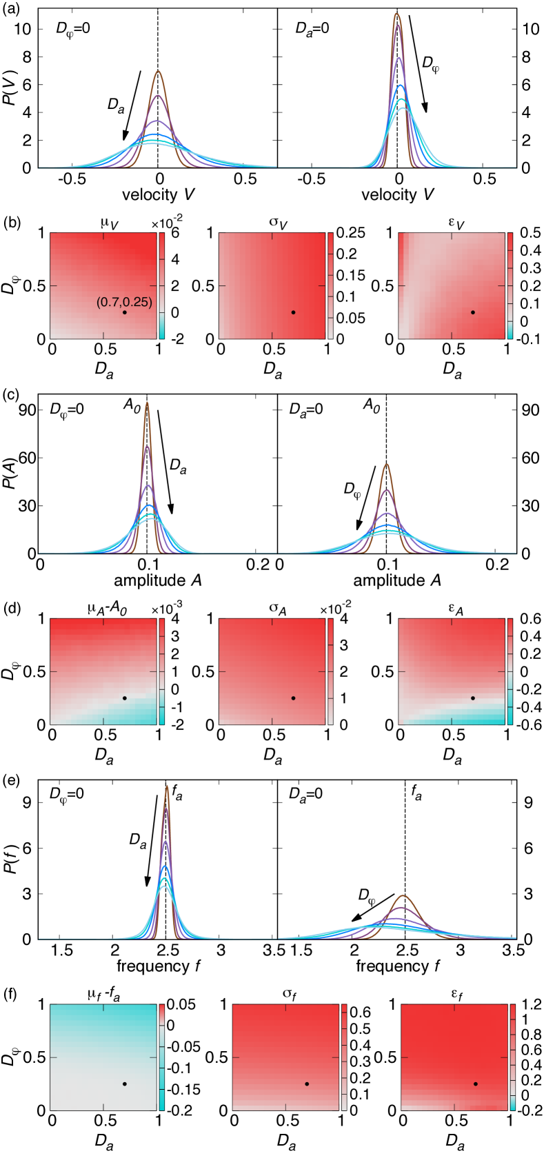
Figure 11: Dependence of the distributions on the noise strengths for $\chi_{c}=0.375,~{}C_{\Gamma}=2.0$, and $f_{a}=2.5$. The distributions and statistical measures of (a)-(b) the thrust velocity $V$, (c)-(d) tailbeat amplitude $A$, and (e)-(f) tailbeat frequency $f$. In (a), (c), (e), the left subplot shows the dependence of the distribution on $D_{a}$ with $D_{\varphi}=0$, and the right subplot is the dependence on $D_{\varphi}$ with $D_{a}=0$. The values of $D_{a}$ or $D_{\varphi}$ are $\{0.05,0.1,0.25,0.5,0.75,1\}$. Larger values of $D_{a}$ or $D_{\varphi}$ give a wider distribution. In (b), (d), (f), the left colormap shows the expected value as a function of $D_{a},~{}D_{\varphi}$, the middle is the standard deviation, and the right is the skewness. The filled circles correspond to $D_{a}=0.7$ and $D_{\varphi}=0.25$, which are mainly the values used in the simulations.

Here, we show the dependence of the distributions on $D_{a}$ and $D_{\varphi}$ in detail. Figs. 11(a), (c), and (e) show the probability distributions of the thrust velocity $V$, tailbeat amplitude $A$, and frequency $f$, respectively, as functions $D_{a}$ or $D_{\varphi}$ (with the increment $\Delta D_{a}=\Delta D_{\varphi}=0.05$). Qualitatively, we find that $P(V)$ is controlled by $D_{a}$ rather than $D_{\varphi}$, while $P(A)$ and $P(f)$ are mainly determined by $D_{\varphi}$. Quantitatively, we define the following statistical measures for $Q=V,A,f$ by using the probability distribution $P(Q)$ Joanes1998 : the expected value

$$\mu_{Q}=\int\differential QP(Q)Q,$$ (78)

the variance

$$\sigma_{Q}^{2}=\int\differential QP(Q)(Q-\mu_{Q})^{2},$$ (79)

where $\sigma_{Q}$ is the standard deviation, and the skewness

$$\varepsilon_{Q}=\frac{1}{\sigma_{Q}^{3}}\int\differential QP(Q)(Q-\mu_{Q})^{3}.$$ (80)

If $\varepsilon_{Q}>0$, the probability distribution has a fat tail at larger $Q$ and vice versa.

The average thrust velocity $\mu_{V}$ is less than 5% of the background flow $U$, but the positiveness of $\mu_{V}$ indicates that noises reduce the thrust speed (see Fig. 11(b)); note that $V>0$ means that the thrust speed is less than $U$. The standard deviation $\sigma_{V}$ depends mainly on $D_{a}$ as expected, and the skewness $\varepsilon_{V}$ is positive.

For the tailbeat amplitude, the deviation from the target amplitude $\mu_{A}-A_{0}$ is less than 5% of $A_{0}$ as shown in Fig. 11(d). The noise strengths $D_{a}$ and $D_{\varphi}$ tend to decrease and increase the amplitude $\mu_{A}$, respectively. Therefore we can tune the noise strengths continuously so that $\mu_{A}\simeq A_{0}$ is always satisfied. On the other hand, for the standard deviation of $A$, there is little difference between its dependences on $D_{a}$ and $D_{\varphi}$. As for the skewness $\varepsilon_{A}$, $D_{\varphi}$ mainly determines its sign, while $D_{a}$ controls its magnitude.

Fig. 11(f) shows the statistical measures for the tailbeat frequency $f$. We find a strong dependence of $P(f)$ on $D_{\varphi}$ rather than on $D_{a}$. The deviation from the input frequency $\mu_{f}-f_{a}$ is always negative and is less than 8% of $f_{a}$, and $\sigma_{f}$ mainly depends on $D_{\varphi}$ as expected. The skewness $\varepsilon_{f}$ is positive.

We adopted $D_{a}=0.7$ and $D_{\varphi}=0.25$ by comparing the distributions with the experimental results (Supplementary Information of Ref. Li2020 ). Figs. 5(b)-(d) show the distributions for these values, which correspond to the filled circles in Figs. 11(b), (d), and (f). The expected values $\mu_{V},~{}\mu_{A},~{}\mu_{f}$ are close to the values $0,~{}A_{0},~{}f_{a}$ for the noiseless case, respectively: $\mu_{V}$ is less than 2% of $U$, $\mu_{A}-A_{0}$ is 0.03% of $A_{0}$, and $\mu_{f}-f_{a}$ is less than 0.15% of $f_{a}$. Our resolution of the noise parameters is such that $\mu_{A}$ changes only 0.1%-0.3% of $A_{0}$ by each step increment $\Delta D_{a}$ and $\Delta D_{\varphi}$. On the other hand, $\mu_{V}$ changes 0.1%-0.2% of $U$, and $\mu_{f}$ changes 0.1%-0.2% of $f_{a}$ by $\Delta D_{a}$ and $\Delta D_{\varphi}$. The height and width of the distributions $P(V),~{}P(A),~{}P(f)$ are qualitatively in good agreement with that of goldfish. Furthermore, the asymmetry of $P(V)$ and $P(f)$ are similar to the experimental results: $P(V)$ has a slightly fat tail on the right sight of the peak, while $P(f)$ has a noticeably fat tail at larger $f$.

Appendix E Energy dissipation rate

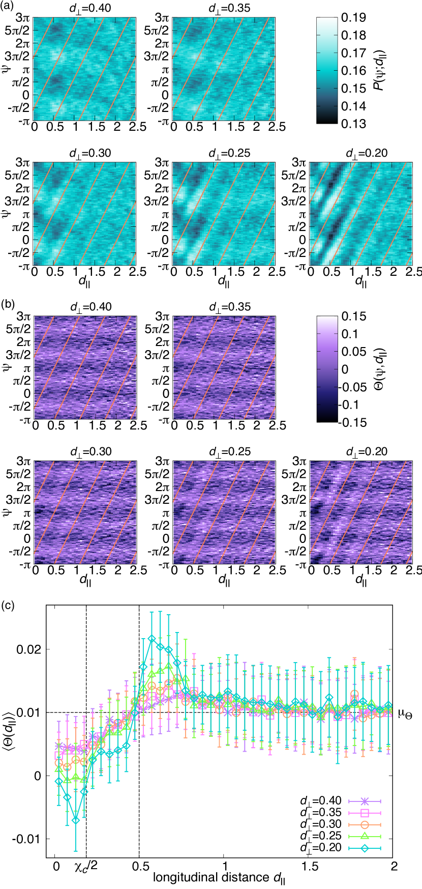
Figure 12: Dependence of (a) the probability distribution $P(\psi;d_{\parallel})$, (b) the dissipation rate $\Theta(\psi,d_{\parallel})$, and (c) $\langle\Theta(d_{\perp})\rangle$ on $d_{\perp}$ with $C_{\Gamma}=2.0$. The display scheme is the same as in Figs. 7(a)-(b) and Fig. 8.

Here we discuss some properties of the energy dissipation rate for pair swimming. In the main text, we fixed the the lateral distance $d_{\perp}=0.2$. Here we show the dependence of $P(\psi;d_{\parallel})$ on $d_{\perp}$ in Fig. 12(a). We find that $P(\psi;d_{\parallel})$ approaches a uniform distribution as $d_{\perp}$ increases to $d_{\perp}=0.4$. The plot of the energy dissipation rate $\Theta(\psi,d_{\parallel})$ in Fig. 12(b) shows only the horizontal stripe pattern for $d_{\perp}=0.4$, and the oblique stripes gradually disappeared with increasing $d_{\perp}$. Also, the expected value $\langle\Theta(d_{\parallel})\rangle$ deviates negatively from $\mu_{\Theta}$ at $d_{\parallel}\lesssim 0.5$ for any value of $d_{\perp}$ (see Fig. 12(c)). This energy gain is larger than the energy consumption in the range $d_{\parallel}\gtrsim 0.5$.

Next we provide an explanation of the horizontal stripe pattern of the dissipation rate $\Theta(\psi,d_{\parallel})$ as seen in Fig. 7(b), using the statistical properties of a solitary swimmer. From Fig. 6(a), we can approximate the phase distribution as

$$P(\phi)\approx\frac{1}{2\pi}+\epsilon\cos(2\phi+\gamma_{P}),$$ (81)

where $\epsilon\sim\mathcal{O}(10^{-3})$ and $\gamma_{P}$ is a constant. In addition, from Fig. 6(b), the dissipation rate $\Theta(\phi)$ is approximated by

$$\Theta(\phi)\approx\Theta_{0}+E\cos(2\phi-\gamma_{\Theta})$$ (82)

where $\Theta_{0}\sim\mathcal{O}(10^{-1})$, $E\sim\mathcal{O}(1)$, and $\gamma_{\Theta}$ is a constant. Using these approximations, a straightforward calculation gives the average dissipation rate as

$$\mu_{\Theta}=\Theta_{0}+\pi E\epsilon\cos(\gamma_{P}+\gamma_{\Theta})\sim\mathcal{O}(10^{-2})>0,$$ (83)

which corresponds to the numerically value $\mu_{\Theta}\simeq 0.01$ (see Fig. 6(b) inset).

Next, we calculate the probability distribution of the phase difference $\psi=\phi_{1}-\phi_{2}$ neglecting the hydrodynamic interaction between the two swimmers. As the distribution does not depend on the distance, we denote $\widetilde{P}(\psi):=P(\psi;d_{\parallel})$ for simplicity. Exploiting the symmetry between $\phi_{1}$ and $\phi_{2}$, or $\psi$ and $-\psi$, we rewrite the joint probability distribution of $\phi_{1}$ and $\phi_{2}$ as

$$P(\phi_{1})P(\phi_{2}) = P(\phi_{1})\frac{1}{2}(P(\phi_{1}+\psi)+P(\phi_{1}-\psi))$$ (84)

$$=: P(\phi_{1},\psi).$$

Then $\widetilde{P}(\psi)$ is obtained by integrating $P(\phi_{1},\psi)$ over the range $\phi_{1}\in[-\pi,\pi]$, which yields

$$\widetilde{P}(\psi)=\frac{1}{2\pi}+\pi\epsilon^{2}\cos 2\psi.$$ (85)

This result indicates that a horizontal stripe pattern emerges in $P(\psi;d_{\parallel})$, but we cannot detect it in Fig. 7(a) due to the smallness of $\epsilon^{2}\sim\mathcal{O}(10^{-6})$.

Finally, we calculate the dissipation rate $\widetilde{\Theta}(\psi):=\Theta(\psi,d_{\parallel})$ in the absence of hydrodynamic interaction. Noting that the probability distribution of $\phi_{1}$ for a given value of $\psi$ is given by $P(\phi_{1},\psi)/\widetilde{P}(\psi)$, we obtain

$$\widetilde{\Theta}(\psi) = \int_{-\pi}^{\pi}\differential\phi_{1}\Theta(\phi_{1})\frac{P(\phi_{1},\psi)}{\widetilde{P}(\psi)}$$ (86)

$$= \Theta_{0}+\pi E\epsilon\cos(\gamma_{P}+\gamma_{\Theta})(1+\cos 2\psi)+\mathcal{O}(\epsilon^{2})$$

$$= \mu_{\Theta}+\pi E\epsilon\cos(\gamma_{P}+\gamma_{\Theta})\cos 2\psi+\mathcal{O}(\epsilon^{2}).$$

Therefore, the energy dissipation rate $\Theta(\psi,d_{\parallel})$ has an ${\cal O}(\epsilon)$ deviation from $\mu_{\Theta}$, which is proportional to $\cos 2\psi$. (Note also that $\cos(\gamma_{P}+\gamma_{\Theta})<0$.) This explains the horizontal stripe pattern in the plots in Fig. 7(b).

In addition, the expected value of $\widetilde{\Theta}(\psi)$ is

$$\langle\Theta\rangle=\int_{-\pi}^{\pi}\differential\psi\widetilde{\Theta}(\psi)\widetilde{P}(\psi)=\mu_{\Theta}+\mathcal{O}(\epsilon^{2}),$$ (87)

and thus is almost equal to $\mu_{\Theta}$, as shown in Fig. 8.

References

- (1) L. Conradt and T. J. Roper, Trends Ecol. Evol. 20, 449 (2005).
- (2) T. Vicsek and A. Zafeiris, Phys. Rep. 517, 71 (2012).
- (3) J. K. Parrish, S. V. Viscido, and D. Grünbaum, Biol. Bull. 202, 296 (2002).
- (4) U. Lopez, J. Gautrais, I. D. Couzin, and G. Theraulaz, Interface Focus 2, 693 (2012).
- (5) K. Terayama, H. Hioki, and M. Sakagami, Int. J. Semant. Comput. 9, 143 (2015).
- (6) R. Harpaz, E. Schneidman, eLife, 9, e56196 (2020).
- (7) J. C. A. Liao, Philos. Trans. R. Soc. B 362, 1973 (2007).
- (8) C. M. Breder, Ecology 35, 361 (1954).
- (9) H. Niwa, J. Theor. Biol. 171, 123 (1994).
- (10) I. Aoki, Bull. Jpn. Soc. Sci. Fish. 48, 1081 (1982).
- (11) A. Huth and C. Wissel, J. Theor. Biol. 156, 365 (1992).
- (12) A. Huth and C. Wissel, Ecol. Model. 75, 135 (1994).
- (13) I. D. Couzin, J. Krause, R. James, G. D. Ruxton, and N. R. Franks, J. Theor. Biol. 218, 1 (2002).
- (14) J. Gautrais, F. Ginelli, R. Fournier, S. Blanco, M. Soria, H. Chaté, and G. Theraulaz, PLOS Comput. Biol. 8, e1002678 (2012).
- (15) D. S. Calovi, U. Lopez, S. Ngo, C. Sire, H. Chaté, and G. Theraulaz, New J. Phys. 16, 015026 (2014).
- (16) A. Filella, F. Nadal, C. Sire, E. Kanso, and C. Eloy, Phys. Rev. Lett. 120, 198101 (2018).
- (17) J. Deng and D. Liu, Bioinspir. Biomim. 16, 046013 (2021).
- (18) S. Ito and N. Uchida, J. Phys. Soc. Jpn. 91, 064806 (2022).
- (19) S. Ito and N. Uchida, Europhys. Lett. 138, 17001 (2022).
- (20) C. K. Hemelrijk and H. Hildenbrandt, Ethology 114, 245 (2008).
- (21) R. Bastien and P. A. Romanczuk, Sci. Adv. 6, eaay0792 (2020).
- (22) A. A. Tchieu, E. Kanso, and P. K. Newton, Proc. R. Soc. A 468, 3006 (2012).
- (23) M. Gazzola, A. A. Tchieu, D. Alexeev, A. de Brauer, and P. Koumoutsakos, J. Fluid Mech. 789, 726 (2016).
- (24) G. V. Lauder and E. G. Drucker, News Physiol. Sci., 17, 235 (2002).
- (25) O. Akanyeti, J. Putney, Y. R. Yanagitsuru, G. V. Lauder, W. J. Stewart, and J. C. Liao, Proc. Natl. Acad. Sci. U.S.A. 114, 13828 (2017).
- (26) T. N. Wise, M. A. B. Schwalbe, and E. D. Tytell, J. Exp. Biol. 221, jeb190892 (2018).
- (27) C. M. Breder, Zoologica 50, 97 (1965).
- (28) D. Weihs, Nature 241, 290 (1973).
- (29) B. L. Partridge and T. J. Pitcher, Nature 279, 418 (1979).
- (30) S. Marras, S. S. Killen, J. Lindström, D. J. McKenzie, J. F. Steffensen, and P. Domenici, Behav. Ecol. Sociobiol. 69, 219 (2014).
- (31) I. Ashraf, R. Godoy-Diana, J. Halloy, B. Collignon, and B. Thiria, J. R. Soc. Interface 13, 20160734 (2016).
- (32) I. Ashraf, H. Bradshawa, T. Ha, J. Halloy, R. Godoy-Diana, and B. Thiria, Proc. Natl. Acad. Sci. U.S.A. 114, 9599 (2017).
- (33) L. Li, M. Nagy, J. M. Graving, J. Bak-Coleman, G. Xie, and I. D. Couzin, Nat. Commun. 11, 5408 (2020).
- (34) G. J. Elfring and E. Lauga, Phys. Rev. Lett. 103, 088101 (2009).
- (35) W. Liao and E. Lauga, Phys. Rev. E 103, 042419 (2021).
- (36) P. A. Dewey, D. B. Quinn, B. M. Boschitsch, and A. J. Smits, Phys. Fluids 26, 041903 (2014).
- (37) B. M. Boschitsch, P. A. Dewey, and A. J. Smits, Phys. Fluids 26, 051901 (2014).
- (38) A. D. Becker, H. Masoud, J. W. Newbolt, M. Shelley, and L. Ristroph, Nat. Commun. 6, 97 (2015).
- (39) S. Ramananarivo, F. Fang, A. Oza, J. Zhang, and L. Ristroph, Phys. Rev. Fluids 1, 071201(R) (2016).
- (40) J. W. Newbolt, J. Zhang, and L. Ristroph, Proc. Natl. Acad. Sci. U.S.A. 46, 2419 (2019).
- (41) A. U. Oza, L. Ristroph, and M. J. Shelley, Phys. Rev. X 9, 041024 (2019).
- (42) X. Zhu, G. He, and X. Zhang, Phys. Rev. Lett. 113, 238105 (2014).
- (43) S. G. Park and H. J. Sung, J. Fluid Mech. 840, 154 (2018).
- (44) Z. Peng, H. Huang, and X. Lu, J. Fluid Mech. 849, 1068 (2018).
- (45) C. K. Hemelrijk, D. A. P. Reid, H. Hildenbrandt, and J. T. Padding, Fish. Fish. 16, 511 (2015).
- (46) M. Daghooghi and I. Borazjani, Bioinspir. Biomim. 10, 056018 (2015).
- (47) A. P. Maertens, A. Gao, and M. S. Triantafyllou, J. Fluid Mech. 813, 301 (2017).
- (48) G. Li, D. Kolomenskiy, H. Liu, B. Thiria, and R. Godoy-Diana, PLOS ONE 14, e0215265 (2019).
- (49) X. Li, J. Gu, Z. Su, and Z. Yao, Phys. Fluids 33, 121905 (2021).
- (50) Y. Pan and H. Dong, Phys. Fluids 34, 111902 (2022).
- (51) J. Kelly, P. Yu, A. Menzer, and D. Haibo, Phys. Fluids 35, 041906 (2023).
- (52) Z. Lin, D. Liang, A. P. S. Bhalla, A. A. S. Al-Shabab, M. Skote, W. Zheng, and Y. Zhang, Phys. Fluids 35, 081901 (2023).
- (53) M. Sfakiotakis, D. M. Lane, and J. B. C. Davies, IEEE J. Ocean. Eng. 24, 237 (1999).
- (54) G. V. Lauder and E. D. Tytell, Fish Physiol. 23, 425 (2005).
- (55) A. Azuma, The Biokinetics of Flying and Swimming (Springer, Tokyo, 1992).
- (56) M. Nagai, I. Teruya, K. Uechi, and T. Miyazato, Trans. Jpn. Soc. Mech. Eng. B 62, 200 (1996). (https://www.jstage.jst.go.jp/article/kikaib1979/62/593/62_593_200/_pdf/-char/en)
- (57) M. Hirayama, T. Nagamatsu, and K. Ueda, Mem. Fac. Fish. Kagoshima Univ. 49, 17 (2000). (https://ir.kagoshima-u.ac.jp/?action=repository_uri&item_id=6287&file_id=16&file_no=1)
- (58) M. Gazzola, M. Argentina, and L. Mahadevan, Proc. Natl. Acad. Sci. U.S.A. 112, 3874 (2015).
- (59) R. E. Jones, R. J. Petrell, and D. Pauly, Aquac. Eng. 20, 216 (1999).
- (60) L. D. Landau and E. M. Lifshitz, Fluid Mechanics (Butterworth-Heinemann, New York, 1987).
- (61) R. Bainbridge, J. Exp. Biol. 35, 109 (1958).
- (62) J. R. Hunter and J. R. Zweifel Fish. Bull. 69, 253 (1971).
- (63) P. W. Webb, P. T. Kostecki, and E. Don Stevens, J. Exp. Biol. 109, 77 (1984).
- (64) G. Li, H. Liu, U. K. Müller, C. J. Voesenek, and J. L. van Leeuwen, Proc. R. Soc. B 288, 20211601 (2021).
- (65) Note that, in the context of experiments of Refs. Bainbridge1958 ; Hunter1971 ; Webb1984 ; Akanyeti2017 ; Li2021 , they measure the peak to peak amplitude as “the amplitude”.
- (66) G. I. Taylor, Proc. Roy. Soc. Lond. A 214, 158 (1952).
- (67) M. J. Lighthill, J. Fluid Mech. 9, 305 (1960).
- (68) L. D. Landau, E. M. Lifshitz, A. M. Kosevich, and L. P. Pitaevskii, Theory of Elasticity (Butterworth-Heinemann, New York, 1986).
- (69) M. J. McHenry, C. A. Pell, and J. H. Long Jr, J. Exp. Biol. 198, 2293 (1995).
- (70) S. Grillner, Neuron 52, 751 (2006).
- (71) J. Song, I. Pallucchi, J. Ausborn, K. Ampatzis, M. Bertuzzi, P. Fontanel, L. D. Picton, and A. El Manira, Neuron 105, 1048 (2020).
- (72) Ö. Ekeberg and S. Grillner, Phil. Trans. R. Soc. Lond. B 354, 895 (1999).
- (73) K. Matsuoka, Biol. Cybern. 104, 297 (2011).
- (74) M. A. B. Schwalbe, A. L. Boden, T. N. Wise, and E. D. Tytell, Sci. Rep. 9, 8088 (2019).
- (75) D. B. Giaiotti and F. Stel, The Rankine vortex model, University of Trieste-International Centre for Theoretical Physics (2006). (https://moodle2.units.it/pluginfile.php/109093/mod_resource/content/1/rankine-vortex-notes.pdf)
- (76) E. G. Drucker and G. V. Lauder, J. Exp. Biol. 202, 2393 (1999).
- (77) T. Schnipper, A. Andersen, and T. Bohr, J. Fluid Mech. 633, 411 (2009).
- (78) N. Agre, S. Childress, J. Zhang, and L. Ristroph, Phys. Rev. Fluids 1, 033202 (2016)
- (79) X. Ortiz, D. Rival, and D. Wood, Energies 8, 2438 (2015).
- (80) C. E. Brennen, A Review of Added Mass and Fluid Inertial Forces (Naval Civil Engineering Laboratory, Port Hueneme, 1982).
- (81) I. Tanaka and M. Nagai, Teikou to suishin no ryuutai rikigaku: suisei seibutsu no kousoku yuuei nouryoku ni manabu, (Ship & Ocean Foundation, Tokyo, 1996). (https://www.spf.org/_opri_media/publication/pdf/199609_rp040220.pdf)
- (82) M. Nagai, Nagare 10, 47 (1979). (https://www.jstage.jst.go.jp/article/nagare1970/10/4/10_4_47/_pdf/-char/en)
- (83) R. Bainbridge, J. Exp. Biol. 40, 23 (1963).
- (84) M. Gazzola, M. Argentina, and L. Mahadevan, Nat. Phys. 10, 758 (2014).
- (85) G. S. Triantafyllou, M. S. Triantafyllou, and M. A. Grosenbaugh, J. Fluids Struct. 7, 205 (1993).
- (86) G. K. Taylor, R. L. Nudds, and A. L. R. Thomas, Nature 425, 707 (2003).
- (87) P. Domenici and R. W. Blake, J. Exp. Biol. 200, 1165 (1997).
- (88) G. Li, I. Ashraf, B. François, D. Kolomenskiy, F. Lechenault, R. Godoy-Diana, and B. Thiria, Commun. Biol. 4, 40 (2021).
- (89) R. E. Shadwick and D. A. Syme, J. Exp. Biol. 211, 1603 (2008).
- (90) V. Di Santo, E. Goerig, D. K. Wainwright, O. Akanyeti, J. C. Liao, T. Castro-Santos, and G. V. Lauder, Proc. Natl. Acad. Sci. U.S.A. 118, e2113206118 (2021).
- (91) L. Wen and G. Lauder, Bioinspir. Biomim. 8, 046013 (2013).
- (92) K. N. Lucas, G. V. Lauder, and E. D. Tytell, Proc. Natl. Acad. Sci. U.S.A. 117, 10585 (2020).
- (93) R. Thandiackal and G. Lauder, eLife 12, e81392 (2023).
- (94) J. C. Nauen and G. V. Lauder, J. Exp. Biol. 205, 1709 (2002).
- (95) N. E. Huang and S. S. P. Shen, Hilbert-Huang Transform and Its Applications (World Scientific, Singapore, 2014).
- (96) H. Jiang, Y. Li, and Z. Cheng, Appl. Mech. Mater. 518, 161 (2014).
- (97) K. Wendel, Hydrodynamic Masses and Hydrodynamic Moments of Inertia (MIT Libraries, Cambridge, 1956).
- (98) G. Di Ilio, D. Chiappini, S. Ubertini, G. Bella, S. Succi, Comput. Fluids 166, 200 (2018).
- (99) T. Tandler, E. Gellman, D. De La Cruz, and D. J. Ellerby, J. Fish Biol. 94, 532 (2019).
- (100) T. Y. Wu, in Scale Effects in Animal Locomotion, ed. T. J. Pedley (Academic Press, New York, 1977) pp. 203.
- (101) D. N. Joanes and C. A. Gill, J. R. Stat. Soc. (Ser. D) 47, 183 (1998).