Optimization of probabilistic quantum search algorithm with a priori information

Abstract

A quantum computer encodes information in quantum states and runs quantum algorithms to surpass the classical counterparts by exploiting quantum superposition and quantum correlation. Grover’s quantum search algorithm is a typical quantum algorithm that proves the superiority of quantum computing over classical computing. It has a quadratic reduction in the query complexity of database search, and is known to be optimal when no a priori information about the elements of the database is provided. In this work, we consider a probabilistic Grover search algorithm allowing nonzero probability of failure for a database with a general a priori probability distribution of the elements, and minimize the number of oracle calls by optimizing the initial state of the quantum system and the reflection axis of the diffusion operator. The initial state and the reflection axis are allowed to not coincide, and thus the quantum search algorithm rotates the quantum system in a three-dimensional subspace spanned by the initial state, the reflection axis and the search target state in general. The number of oracle calls is minimized by a variational method, and formal results are obtained with the assumption of low failure probability. The results show that for a nonuniform a priori distribution of the database elements, the number of oracle calls can be significantly reduced given a small decrease in the success probability of the quantum search algorithm, leading to a lower average query complexity to find the solution of the search problem. The results are applied to a simple but nontrivial database model with two-value a priori probabilities to show the power of the optimized quantum search algorithm. The paper concludes with a discussion about the generalization to higher-order results that allows for a larger failure probability for the quantum search algorithm.

I Introduction

Quantum computing has been expected to revolutionize the field of computing since it was proposed [1, 2]. It accelerates computing tasks by taking advantage of the nonclassicalities of quantum systems such as quantum superposition and quantum correlation. With the development of quantum computing, various quantum algorithms have been proposed. The large number factorization algorithm proposed by Peter W. Shor [3, 4] has an exponential speedup compared to classical factorization algorithms, and the quantum search algorithm proposed by Lov K. Grover [5, 6] has a quadratic speedup in terms of the database size compared to classical database search algorithms. More quantum algorithms have been proposed in recent years, such as the variational quantum eigensolver algorithm [7] and the quantum approximate optimization algorithms [8] for noisy intermediate-scale quantum devices, the Harrow-Hassidim-Lloyd algorithm for linear systems of equations applicable to quantum machine learning [9], the boson sampling [10] for photon distribution in linear optics, etc.

For a classical database with $N$ elements, if a search task has $M$ solutions, the classical query complexity of finding a solution is usually of order $O(N/M)$. In quantum computing, Grover’s search algorithm finds a solution in a database by preparing the quantum system in an appropriate superposed state of the computational basis and driving the system to approach a target state with alternate oracle operations and specific diffusion operations. After the evolution, a quantum projective measurement is performed along the computational basis on the system to obtain the target state. The query complexity required by Grover’s search algorithm is $O(\sqrt{N/M})$, which is a quadratic speedup compared to a classical search algorithm. Because of this superiority, quantum search algorithms have been found useful in various applications, such as quantum dynamic programming [11], quantum random-walk search algorithm [12], the preparation of Greenberger-Horne-Zeilinger states using algorithms [13], etc.

While the quantum search algorithm has found wide applications in vast areas, the algorithm itself can still be extended and improved in various aspects. For example, the quantum partial search algorithm [14, 15, 16, 17, 18, 19, 20] decomposes the database into smaller blocks and searches for the block which the target state belongs to instead of finding the exact location of the target state. Another idea is to change the Grover iterations of the quantum search algorithm. The core of Grover’s quantum search algorithm is the amplitude amplification technique [21, 22] which increases the weight of the search target in the superposed state of the quantum system by repetition of the Grover iteration consisting of the oracle operation and a diffusion operation. It has been proposed that the diffusion operation in the Grover iteration can be replaced by a two-dimensional phase rotation [23]. Extension of the two-dimensional phase rotation to a three-dimensional rotation was subsequently proposed, and a phase matching condition to realize the quantum search algorithm by phase rotation was found [24, 25, 26]. This phase-matching condition has been verified theoretically [27, 23], and realized by experiments on optical systems [28, 29] and ion trap systems[30], etc. An interesting zero-failure quantum search algorithm based on this condition was subsequently proposed by Long [31], and this algorithm has been applied in different quantum tasks, such as quantum pattern recognition [32], sliding mode control of quantum systems [33] and quantum image compression [34]. Recently, an improved two-parameter modified version [35] was proposed to realize deterministic search without user control of the quantum oracle. More variants of the quantum search algorithm have also been proposed, such as the quantum search algorithm with continuous variables [36, 37, 38], the fixed-point quantum search algorithm [39, 40], the Hamiltonian search algorithm [38], etc. A review of extended quantum search algorithms can be referred to [41, 42, 43, 44, 45]. Moreover, the quantum search algorithm has been realized experimentally on various physical systems, including photons [46, 47], superconducting circuits [48, 49], nuclear magnetic resonance [50, 51, 52], trapped ions [53, 54], etc.

The lower bounds for the number of oracle calls of these algorithms have been proven optimal [55, 56, 57]. In the optimality of the quadratic speedup of Grover’s search algorithm, a key ingredient is that all the elements of the database are equally likely to be the solution of the search problem. If the elements of the database are allowed to be unequally likely to be the search solution, the result can be quite different, as it can be expected that preparing the quantum system closer to the states with higher probabilities to be the search target will be more beneficial to the search algorithm [58, 59, 60, 61]. An intuitive example is that, if some of the database elements, e.g., $K$ of the $N$ elements, are known to have very low probabilities (or even zero probabilities) to be the search target, one just needs to prepare the quantum system in a superposition of the remaining $N-K$ elements and flip the system around this state as well in the Grover iterations, and then the query complexity will be reduced to $O(\sqrt{N-K})$ rather than $O(\sqrt{N})$ at the cost of a low probability to fail the search task. This inspires us to consider the following question: if we know in advance the a priori probabilities of the elements in the database to be the search target, what is the optimal performance of the quantum search algorithm obtained by exploiting the a priori probabilities of the database elements and allowing the algorithm to succeed probabilistically?

The purpose of this work is to study the minimal query complexity of the quantum search algorithm by optimizing the initial state of the quantum system and the reflection axis of the diffusion operator given the average success probability of the algorithm. The query complexity is quantified by the number of oracle calls, and the minimization of the query complexity is carried out by variation of the initial state of the quantum system and the reflection axis of the diffusion operator. The optimization conditions turn out to be highly nontrivial and hard to solve in general. However, if the failure probability is low, one can expect that the optimal initial state and the optimal reflection axis should just deviate slightly from the uniformly superposed state of all database elements as in the original Grover search algorithm. This leads to a differential approach to solving the optimization equations: by taking the differentiation of the optimization equations as well as the normalization conditions for the initial state and the reflection axis, one can establish a differential relation between the success probability of the algorithm, the number of the oracle calls, the optimal initial state of the system and the optimal reflection axis of the diffusion operator. When the failure probability of the algorithm is low, this differential relation can approximately tell the reduction of the number of oracle calls in terms of the failure probability of the quantum search algorithm.

In this work, based on the above idea, we obtain a formal second-order differential relation between the failure probability of the algorithm and the reduction in the number of oracle calls given a general a priori probability distribution of the database elements. An interesting property of the result is that the reduction percentage of the number of oracle calls is proportional to the square root of the failure probability of the quantum search algorithm which is always much larger than the failure probability when the latter is small, implying the optimized probabilistic quantum search algorithm can decrease the average number of oracle calls when the success probability of the algorithm is taken into account. The formal results are applied to a simple but nontrivial database model where all the elements have only two possible values for the a priori probabilities, and the reduction of the query complexity is analytically derived in terms of the failure probability of the search algorithm and illustrated in detail by numerical computation.

The paper is structured as follows. In Sec. II, we give a brief overview for Grover’s quantum search algorithm. In Sec. III, the number of oracle calls is minimized by the method of Lagrange multipliers given the a priori probabilities of the database elements and the success probability of the search algorithm. The failure probability of the algorithm is then assumed to be small, and the reduction of the number of oracle calls is obtained in terms of the failure probability by differentiating the optimization equations. Sec. IV is devoted to a simple database model with the a priori probabilities of the elements taken to be two valued. The paper finally concludes in Sec. V with a summary of the work and a discussion of the generalization to higher order results that allow for a larger failure probability of the quantum search algorithm.

II Preliminaries

In this section, we briefly introduce the preliminaries of Grover’s quantum search algorithm [5, 6] relevant to the current research. We focus on the case that the search problem has only one solution throughout this paper.

II.1 Procedures of Grover’s search algorithm

Suppose we have a database with $N$ elements where the probabilities of the elements being the search target are the same, and we use the computational basis of a quantum system to represent the elements of the database. The quantum system is initially prepared in a uniform superposed state,

$$\left|\psi_{0}\right\rangle=\sum_{i=1}^{N}\frac{1}{\sqrt{N}}\left|i\right\rangle.$$ (1)

The solution of the search problem is recognized by a quantum oracle. The quantum oracle can be regarded as a black box, the internal working mechanism of which is not critical to the search algorithm, but can perform a unitary transformation on the quantum system and mark up the solution of the search task by shifting the phase of the target state. In detail, the unitary transformation of the quantum oracle can be written as

$$O=I-2|t\rangle\langle t|,$$ (2)

where $|t\rangle$ is the target state and $I$ is the identity operator on the $N$-dimensional Hilbert space of the system. The effect of the oracle $O$ when it acts on a quantum state is that

$$O|t\rangle=-|t\rangle,\;O|i\rangle=|i\rangle,\;i\neq t.$$ (3)

So, it flips the sign of the target state and leaves the basis states other than the target state unchanged.

While the oracle can mark up the solution by changing the sign of the target state, it cannot lead the quantum system to approach the target state alone as it does not change the amplitude distribution of different basis states in the superposed state of the quantum system. In order to increase the amplitude of the target state in the superposed state of the quantum system, the oracle operation needs to be followed by another unitary transformation, usually called the Grover diffusion operator, which reflects the state of the quantum system around the uniformly superposed state $|\psi_{0}\rangle$,

$$D=2|\psi_{0}\rangle\langle\psi_{0}|-I.$$ (4)

The effect of the diffusion operator $D$ is to invert the amplitudes of the basis states in the superposed state of the system around the mean of all amplitudes. The combination of the oracle $O$ and the diffusion operator $D$ is usually called the Grover operator or Grover iteration, defined as

$$G=DO.$$ (5)

It turns out that the Grover operator $G$ can boost the amplitude of the target state in the superposed state of the system. So if one repeats this procedure for a proper number of times, the quantum system can finally approach the target state of the search problem with a high fidelity.

Grover’s search algorithm has an intuitive geometric interpretation. In order to see how Grover’s algorithm works in the geometric picture, the initial state can be rewritten as

$$\begin{aligned} |\psi_{0}\rangle=&a_{t}\left|t\right\rangle+\sum_{i\neq t}^{N}a_{i}\left|i\right\rangle=\sin\theta\left|t\right\rangle+\cos\theta\left|t_{\perp}\right\rangle,\end{aligned}$$ (6)

where the state is decomposed to two states, one the target state $|t\rangle$ and the other a uniformly superposed state in the remaining $(N-1)$-dimensional subspace orthogonal to the target state $t$, and

$$\sin\theta=\frac{1}{\sqrt{N}},\;\cos\theta=\sqrt{1-\frac{1}{N}}.$$ (7)

It can be verified that after $j$ repetitions of the Grover iteration, the initial state of the quantum system is transformed to

$$\begin{aligned} |\psi_{j}\rangle=&\sin\left(2j+1\right)\theta\left|t\right\rangle+\cos\left(2j+1\right)\theta\left|t_{\perp}\right\rangle\end{aligned}.$$ (8)

So, it can be seen that the state of the quantum system always lies in the two-dimensional subspace spanned by $|t\rangle$ and $|t_{\perp}\rangle$ during the repetitions of the Grover iteration, and the effect of the algorithm is essentially to rotate the quantum system from the initial state $|\psi\rangle$ towards the target state $t$.

The geometric picture of Grover’s algorithm is illustrated in Fig. 1.

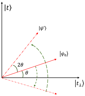
Figure 1: Sketch of the standard Grover quantum search algorithm. The initial state of the quantum system and the reflection axis of the diffusion operator are both the uniform superposed state $|\psi_{0}\rangle$ of all database elements. The initial state $|\psi_{0}\rangle$ and the target state $|t\rangle$ of the search problem span a two-dimensional subspace. The Grover iteration consists of two steps: First perform the oracle operation which reflects the system about the state $|t_{\perp}\rangle$ that is orthogonal to the target state $|t\rangle$ in the two-dimensional subspace, and then perform the diffusion operation which reflects the system about the state $|\psi_{0}\rangle$. The total effect of the Grover iteration is to rotate the system in the two-dimensional subspace away from $|t_{\perp}\rangle$ by double the angle between $|\psi_{0}\rangle$ and $|t_{\perp}\rangle$.

II.2 Query complexity of Grover’s search algorithm

After the evolution, one measures the quantum system along the computational basis. If the system collapses to the target state, the search task is completed successfully. In order to obtain the solution of the search problem with a high probability, the quantum system should be as close to the target state as possible at the end of the evolution. Ideally, one expects to have the probability of obtaining the target state

$$P_{j}=\left|\langle t|\psi_{j}\rangle\right|^{2}=\sin^{2}\left(2j+1\right)\theta=1,$$ (9)

so the optimal number of Grover iterations is

$$j=\frac{\pi}{4\arcsin\frac{1}{\sqrt{N}}}-\frac{1}{2}.$$ (10)

When the size of the database, $N$, is large, $j$ can be approximated as

$$j\approx\frac{\pi}{4}\sqrt{N}.$$ (11)

In reality, as the number of Grover iterations needs to be an integer, $j$ can usually be chosen as

$$j\approx\left\lceil\frac{\pi}{4}\sqrt{N}\right\rceil,$$ (12)

where $\left\lceil x\right\rceil$ is the ceiling function which outputs the minimum integer that is no smaller than $x$.

III Optimization method

When the elements of a database are equally likely to be the solution of the search problem, Grover’s quantum search algorithm has been proven to be optimal in the query complexity. However, if the elements have a nonuniform a priori probability distribution to be the search target, Grover’s algorithm can be further improved, as one may increase the weights of the basis states with higher probabilities in the initial state of the quantum system so that the system can approach the target state faster.

In this section, we study the minimization of the query complexity of Grover’s quantum search algorithm by optimizing the initial state of the system and the reflection axis of the diffusion operator, provided the average success probability of the algorithm to find the solution is given.

III.1 Success probability of generalized Grover search algorithm

Consider a database of $N$ items, the a priori probabilities of which to be the search target is known. Denote the a priori probability of the $k$th element to be search target as $p_{k}$, and the probabilities $p_{k}$, $k=1,\cdots,N$, are normalized,

$$p_{1}+\cdots+p_{N}=1.$$ (13)

In contrast to the uniformly superposed initial state in the standard Grover quantum search algorithm, a nonuniformly superposed initial state of the quantum system may perform better when the a priori probabilities of the database elements are given, as one may increase the weights of the basis states with higher a priori probabilities to accelerate the search algorithm. So, we assume the initial state of the quantum system to be an arbitrary state in the current problem, i.e.,

$$\left|\psi\right\rangle=\sum_{i=1}^{N}a_{i}\left|i\right\rangle,$$ (14)

where $a_{i}$’s are arbitrary coefficients that satisfy the normalization condition,

$$|a_{1}|^{2}+\cdots|a_{N}|^{2}=1.$$ (15)

Similarly, the reflection axis of the diffusion operator is not necessarily the uniformly superposed state, as one may choose the reflection axis to make the diffusion more beneficial to those basis states with higher a priori probabilities, so the reflection axis is also assumed to be an arbitrary state in the current problem, i.e.,

$$\left|\varphi\right\rangle=\sum_{i=1}^{N}b_{i}\left|i\right\rangle,$$ (16)

where $b_{i}$’s are arbitrary coefficients satisfying the normalization condition,

$$|b_{1}|^{2}+\cdots|b_{N}|^{2}=1.$$ (17)

As the initial state of the system and the reflection axis of the diffusion operator do not necessarily coincide, the state is no longer rotating in a two-dimensional subspace during the Grover iterations as in the standard Grover search algorithm. In contrast, the initial state of the quantum system can now be decomposed into two orthogonal components, one lying in the two-dimensional subspace spanned by the target state and the reflection axis of the diffusion operator and the other orthogonal to the two-dimensional subspace. The parallel component (that lies within the two-dimensional subspace) is still rotating in the two-dimensional subspace towards the target state by Grover iterations, but the orthogonal component is just flipped about the two-dimensional subspace by each Grover iteration and always kept orthogonal to the two-dimensional subspace. So, we only need to consider the parallel component of the system state in computing the success probability of the algorithm in the following. The mechanism of how the system state is changed by the generalized Grover iterations is illustrated in Fig. 2.

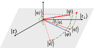
Figure 2: Sketch of the improved quantum search algorithm. The initial state $|\psi\rangle$ of the quantum system and the reflection axis $|\varphi\rangle$ of the diffusion operator are assumed to be arbitrary and do not necessarily coincide. The reflection axis $|\varphi\rangle$ and the solution state $|t\rangle$ of the search problem span a two-dimensional subspace, and the state of the quantum system can be decomposed into two components, $|\psi_{t}^{\parallel}\rangle$ parallel to this two-dimensional subspace and $|\psi_{t}^{\perp}\rangle$ orthogonal to it. The Grover iteration consists of two steps: First perform the oracle operation which reflects the system about the state $|t_{\perp}\rangle$ that is orthogonal to the target state $|t\rangle$ in the two-dimensional subspace, and then perform the diffusion operation which reflects the system about the reflection axis $|\varphi\rangle$. The total effect of the Grover iteration is to rotate the parallel component $|\psi_{t}^{\parallel}\rangle$ of the system state in the two-dimensional subspace which is similar to the original Grover search algorithm but with an additional flip of the orthogonal component $|\psi_{t}^{\perp}\rangle$ about the two-dimensional subspace.

In order to obtain the parallel component of the system state, we need to first find the projector onto the two-dimensional subspace spanned by the target state $|t\rangle$ and the reflection axis $|\varphi\rangle$. The projection operator can be derived by the Gram-Schmidt orthogonalization of $|t\rangle$ and $|\varphi\rangle$, and the result turns out to be

$$P_{t}=\frac{\lvert t\rangle\langle t\lvert+\lvert\varphi\rangle\langle\varphi\lvert-\lvert t\rangle\langle\varphi\lvert\langle t\lvert\varphi\rangle-\lvert\varphi\rangle\langle t\lvert\langle\varphi\lvert t\rangle}{1-\left|\langle t\lvert\varphi\rangle\right|^{2}},$$ (18)

where the subscript $t$ of the projection operator $P_{t}$ denotes that the projection operator depends on the target state $|t\rangle$. With this projection operator, the parallel component of the system initial state $|\psi\rangle$ can be obtained as

$$|\psi_{t}^{\parallel}\rangle=P_{t}|\psi\rangle=\sqrt{\langle\psi|P_{t}|\psi\rangle}(\sin\phi_{0}^{t}\left|t\right\rangle+\cos\phi_{0}^{t}\left|t^{\perp}\right\rangle),$$ (19)

where $\left|t^{\perp}\right\rangle$ is the state orthogonal to the target state $|t\rangle$ in the two-dimensional subspace and $\phi_{0}^{t}$ is the initial angle between the parallel component and $\left|t^{\perp}\right\rangle$,

$$\phi_{0}^{t}=\arcsin\frac{\langle t|P_{t}\lvert\psi\rangle}{\sqrt{\langle\psi|P_{t}|\psi\rangle}}.$$ (20)

Therefore, if the target state of the search problem is $|t\rangle$, the success probability to find the system in the target state after $j$ repetitions of the generalized Grover iteration is

$$P_{\mathrm{sus}}^{(t)}=\langle\psi|P_{t}\lvert\psi\rangle\sin^{2}\left(2j\beta_{t}+\phi_{0}^{t}\right),$$ (21)

where $\beta_{t}=\arcsin\langle t\lvert\varphi\rangle$ is the rotation angle of the system state by a single Grover iteration, and both the probability of projecting the system state onto the two-dimensional subspace and the success probability of the final measurement to find the target state are considered. If we also take the a priori probabilities of different database items into account, the final success probability of the generalized Grover search algorithm turns to be

$$\bar{P}= \sum_{t}p_{t}P_{\mathrm{sus}}^{(t)}=\sum_{t}p_{t}\langle\psi|P_{t}|\psi\rangle$$ (22)

$$\times\sin^{2}\left(2j\arcsin\langle t\lvert\varphi\rangle+\arcsin\frac{\langle t|P_{t}|\psi\rangle}{\sqrt{\langle\psi|P_{t}|\psi\rangle}}\right).$$

Eq. (22) will be critical to the optimization of Grover’s search algorithm below.

III.2 Optimization conditions

Now, we proceed to find the minimum number of oracle calls that can drive the quantum system to the target state. It can be verified that the standard Grover search algorithm is always optimal, whatever the a priori probabilities of the database items are, provided the success probability of the search algorithm is required to be $1$ (neglecting the integer nature of the number of the oracle calls). Therefore, we allow a nonzero failure probability of the search algorithm in this work, and investigate how the reduction in the number of oracle calls can compensate for the loss in the success probability of the search algorithm.

Suppose the success probability of the search algorithm is fixed as $P_{0}$ and the number of oracle calls to realize this success probability of the search algorithm is $j$. By the Lagrange multiplier method, we can minimize the number of oracle calls $j$ by letting the variation of the following function be zero,

$$F=j^{2}+\mu\left(\bar{P}-P_{0}\right)+\nu_{1}\left(\langle\psi|\psi\rangle-1\right)+\nu_{2}\left(\langle\varphi|\varphi\rangle-1\right),$$ (23)

where $\mu$, $\nu_{1}$ and $\nu_{2}$ denote the Lagrange multipliers for the constraint conditions of the success probability, the normalization of the initial state and the normalization of the reflection axis of the diffusion operator respectively. Note that $j$ must be positive, so we minimize $j^{2}$ instead of $j$ in the above function (otherwise the variation may generate a negative $j$ with the absolute value minimized).

The number of oracle calls $j$ also needs to be varied in the variation of $F$; however, the discreteness of $j$ makes the variation of $j$ difficult. To circumvent this issue, we assume the number of the database elements $N$ is large and renormalize the number of oracle calls to

$$\lambda=2j\arcsin\frac{1}{\sqrt{N}},$$ (24)

which is still discrete in principle but can vary approximately in a continuous way when $N$ is sufficiently large. The optimized $\lambda$ and the corresponding $j$ will generally be a float number, but one just needs to take the ceiling function of $j$ to make $j$ an integer which will change $j$ by no more than $1$, a negligible change when $N$ is large, so we will just assume $\lambda$ to be a continuous positive number in the following computation. The average success probability $\bar{P}$ of the generalized Grover search algorithm can be rewritten in terms of $\lambda$ as

$$\bar{P}= \sum_{t}\left[p_{t}\langle\psi|P_{t}|\psi\rangle\right.$$ (25)

$$\left.\times\sin^{2}\left(\lambda\frac{\arcsin\langle t\lvert\varphi\rangle}{\arcsin\frac{1}{\sqrt{N}}}+\arcsin\frac{\langle t|P_{t}|\psi\rangle}{\sqrt{\langle\psi|P_{t}|\psi\rangle}}\right)\right],$$

and the $j^{2}$ term in $F$ (23) should be replaced by $\lambda^{2}/(4\arcsin^{2}\frac{1}{\sqrt{N}})$ in this case.

The variation of $F$ includes the variation of the average success probability as well as the other constraint conditions. Since the average success probability is the main constraint condition in the variation of $F$, we study the variation of the success probability $\bar{P}$ first. By some computation, the variation of $\bar{P}$ can be written as

$$\delta\bar{P}=\langle\delta\psi|\text{{\hbox{a_{\psi}\rangle}}}+\langle\delta\varphi|\text{{\hbox{b_{\varphi}\rangle}}}+c_{\lambda}\delta\lambda.$$ (26)

As the expressions for $|a_{\psi}\rangle$, $|b_{\varphi}\rangle$ and $c_{\lambda}$ are quite lengthy, we leave the details to Appendix A.

In Eq. (26), there should have been Hermitian conjugate terms of $\langle\delta\psi|\text{$a_{\psi}\rangle$}$ and $\langle\delta\varphi|\text{$b_{\varphi}\rangle$}$ in the variation of $\bar{P}$ (26), but note that both $|\psi\rangle$ and $|\varphi\rangle$ must be real states, so there are only $\langle\delta\psi|a_{\psi}\rangle$ and $\langle\delta\varphi|b_{\varphi}\rangle$ in Eq. (26). The reality of $|\psi\rangle$ and $|\varphi\rangle$ is not a simplification here, but rather a property of the current method: We start from the average success probability of the quantum search algorithm and optimize the number of Grover iterations by a variational approach, which will be further solved by a differential method below that takes the standard Grover algorithm as the initial parameters. Since the average success probability, the variational approach and the differential method do not introduce any imaginary coefficients and the standard Grover algorithm also does not include any imaginary parameters, the resulted optimal initial state $|\psi\rangle$ and reflection axis $|\varphi\rangle$ must always be real. Hence, the Hermitian conjugates of $\langle\delta\psi|a_{\psi}\rangle$ and $\langle\delta\varphi|b_{\varphi}\rangle$ coincide with themselves.

Taking the other two constraint conditions as well as the $\lambda^{2}$ term into account, the full variation of $F$ can be obtained as

$$\delta F= \langle\delta\psi|(2\nu_{1}|\psi\rangle+\mu|a_{\psi}\rangle)+\langle\delta\varphi|(2\nu_{2}|\varphi\rangle+\mu|b_{\varphi}\rangle)$$ (27)

$$+\left(\mu c_{\lambda}+\frac{\lambda}{2\arcsin^{2}\frac{1}{\sqrt{N}}}\right)\delta\lambda.$$

When the number of oracle calls is minimized, the variation of $F$ should be zero, so this immediately leads to the following optimization equations for the initial state $|\psi\rangle$, the reflection axis $|\varphi\rangle$ of the diffusion operator, and the renormalized number of oracle calls $\lambda$,

$$2\nu_{1}|\psi\rangle+\mu|a_{\psi}\rangle =0,$$ (28)

$$2\nu_{2}|\varphi\rangle+\mu|b_{\varphi}\rangle =0,$$

$$\mu c_{\lambda}+\frac{2\lambda}{4\arcsin^{2}\frac{1}{\sqrt{N}}} =0.$$

Since $\mu$ can be chosen arbitrarily by changing $\nu_{1}$ and $\nu_{2}$ accordingly in the first two equations of (28), the third equation can then always be satisfied and does not need to be further considered in the following computation.

By projecting the first two lines of (28) onto the state $|\psi\rangle$ and $|\varphi\rangle$ respectively, one can obtain the Lagrange multipliers $\nu_{1}$ and $\nu_{2}$,

$$\nu_{1}=-\frac{\mu}{2}\langle\psi|a_{\psi}\rangle,\;\nu_{2}=-\frac{\mu}{2}\langle\varphi|b_{\varphi}\rangle.$$ (29)

Therefore, the optimization equations for $|a_{\psi}\rangle$ and $|b_{\varphi}\rangle$ can be finally obtained as

$$|a_{\psi}\rangle =\langle\psi|a_{\psi}\rangle|\psi\rangle,$$ (30)

$$|b_{\varphi}\rangle =\langle\varphi|b_{\varphi}\rangle|\varphi\rangle.$$

implying the proportionality between $|a_{\psi}\rangle$ and $|\psi\rangle$ and between $|b_{\varphi}\rangle$ and $|\varphi\rangle$.

Eq. (30) is the optimization condition derived from the Lagrange multipliers method for the initial state of the system, the reflection axis of the diffusion operator and the renormalized number of oracle calls. It will be the starting point of the study in the following sections, from which one can obtain the minimal number of oracle calls given the success probability of the search algorithm and the corresponding optimized initial state and reflection axis.

III.3 Differential solution to optimization equations

Solving Eq. (30) is generally difficult, as the equation is nonlinear with respect to the initial state, the reflection axis and the renormalized number of oracle calls. In order to simplify the problem, we assume the failure probability of the algorithm is low, i.e., the success probability $\bar{P}$ is close to $1$, so that the renormalized number of oracle calls and the initial state and the reflection axis have only slight deviations from those of the standard Grover search algorithm. In this case, we just need to obtain the differential relation between the initial state, the reflection axis and the renormalized number of oracle calls to minimize the query complexity of the quantum search algorithm.

In the following, we give a formal differential solution to the optimization problem based on this idea. In detail, one can take the differentiation of Eq. (30), which produces

$$|da_{\psi}\rangle =\langle d\psi|a_{\psi}\rangle|\psi\rangle+\langle\psi|da_{\psi}\rangle|\psi\rangle+\langle\psi|a_{\psi}\rangle|d\psi\rangle,$$ (31)

$$|db_{\varphi}\rangle =\langle d\varphi|b_{\varphi}\rangle|\varphi\rangle+\langle\varphi|db_{\varphi}\rangle|\varphi\rangle+\langle\varphi|b_{\varphi}\rangle|d\varphi\rangle.$$

Projecting these two equations onto $|\psi\rangle$ and $|\varphi\rangle$ respectively, one can obtain $\langle d\psi|a_{\psi}\rangle=0$ and $\langle d\varphi|b_{\varphi}\rangle=0$ by noting that $\langle\psi|d\psi\rangle=0$ and $\langle\varphi|d\varphi\rangle=0$ as $|\psi\rangle$ and $|\varphi\rangle$ are real and normalized states. Hence, the above two differential equations can be simplified to

$$\left(I-|\psi\rangle\langle\psi|\right)|da_{\psi}\rangle =\langle\psi|a_{\psi}\rangle|d\psi\rangle,$$ (32)

$$\left(I-|\varphi\rangle\langle\varphi|\right)|db_{\varphi}\rangle =\langle\varphi|b_{\varphi}\rangle|d\varphi\rangle,$$

where $I$ denotes the $N\times N$ identity matrix.

The explicit results of $|a_{\psi}\rangle$ and $|b_{\varphi}\rangle$ can be derived from the variation of the average success probability $\bar{P}$ as defined in Eq. (26) and are shown in detail in Appendix A, so their differentials $|da_{\psi}\rangle$ and $|db_{\varphi}\rangle$ can be obtained accordingly, which can be further expanded to the differentials of $|\psi\rangle$, $|\varphi\rangle$ and $\lambda$,

$$|da_{\psi}\rangle=A_{\psi\psi}|d\psi\rangle+A_{\psi\varphi}|d\varphi\rangle+d\lambda|a_{\psi\lambda}\rangle,$$ (33)

where $A_{\psi\psi}$ and $A_{\psi\varphi}$ are both $N\times N$ matrices and $|a_{\psi\lambda}\rangle$ is an unnormalized $N\times 1$ vector. Plugging Eq. (33) into the first line of (32), one can have

$$\left(I-|\psi\rangle\langle\psi|\right)|da_{\psi}\rangle= \left(I-|\psi\rangle\langle\psi|\right)A_{\psi\psi}|d\psi\rangle$$ (34)

$$+\left(I-|\psi\rangle\langle\psi|\right)A_{\psi\varphi}|d\varphi\rangle$$

$$+\left(I-|\psi\rangle\langle\psi|\right)d\lambda|a_{\psi\lambda}\rangle$$

$$= \langle\psi|a_{\psi}\rangle|d\psi\rangle.$$

which can be rearranged to

$$\widetilde{A_{\psi}}|d\psi\rangle+\widetilde{A_{\varphi}}|d\varphi\rangle=d\lambda|v_{a}\rangle,$$ (35)

where

$$\widetilde{A_{\psi}} =\langle\psi|a_{\psi}\rangle I-\left(I-|\psi\rangle\langle\psi|\right)A_{\psi\psi},$$ (36)

$$\widetilde{A_{\varphi}} =-\left(I-|\psi\rangle\langle\psi|\right)A_{\psi\varphi},$$

$$|v_{a}\rangle =\left(I-|\psi\rangle\langle\psi|\right)|a_{\psi\lambda}\rangle.$$

Similarly, the differential $|db_{\varphi}\rangle$ can also be expanded to the differentials of $|\psi\rangle$, $|\varphi\rangle$ and $\lambda$,

$$|db_{\varphi}\rangle=B_{\varphi\psi}|d\psi\rangle+B_{\varphi\varphi}|d\varphi\rangle+d\lambda|b_{\varphi\lambda}\rangle,$$ (37)

where $B_{\varphi\psi}$ and $B_{\varphi\varphi}$ are $N\times N$ matrices and $|b_{\varphi\lambda}\rangle$ is an unnormalized $N\times 1$ vector. Plugging Eq. (37) into the second line of (32) and rearranging the equation gives

$$\widetilde{B_{\varphi}}|d\varphi\rangle+\widetilde{B_{\psi}}|d\psi\rangle=d\lambda|v_{b}\rangle,$$ (38)

where

$$\widetilde{B_{\psi}} =-\left(I-|\varphi\rangle\langle\varphi|\right)B_{\varphi\psi},$$ (39)

$$\widetilde{B_{\varphi}} =\langle\varphi|b_{\varphi}\rangle I-\left(I-|\varphi\rangle\langle\varphi|\right)B_{\varphi\varphi},$$

$$|v_{b}\rangle =\left(I-|\varphi\rangle\langle\varphi|\right)|b_{\varphi\lambda}\rangle.$$

Now, the two optimization conditions in Eq. (32) can be merged and written in a more compact way,

$$\begin{aligned} M\begin{bmatrix}|d\psi\rangle\\ |d\varphi\rangle\end{bmatrix}=\begin{bmatrix}|v_{a}\rangle\\ |v_{b}\rangle\end{bmatrix}d\lambda\end{aligned},$$ (40)

where $M$ is a $2N\times 2N$ matrix,

$$M=\begin{bmatrix}\widetilde{A_{\psi}}&\widetilde{A_{\varphi}}\\ \widetilde{B_{\psi}}&\widetilde{B_{\varphi}}\end{bmatrix}.$$ (41)

Therefore, $|d\psi\rangle$ and $|d\varphi\rangle$ is given by

$$\begin{bmatrix}|d\psi\rangle\\ |d\varphi\rangle\end{bmatrix}=M^{-1}\begin{bmatrix}|v_{a}\rangle\\ |v_{b}\rangle\end{bmatrix}d\lambda.$$ (42)

This is the formal differential relation between $|\psi\rangle$, $|\varphi\rangle$ and $\lambda$.

With this differential relation, $|da_{\psi}\rangle$ (33) and $|db_{\varphi}\rangle$ (37) can be written as

$$\begin{bmatrix}|da_{\psi}\rangle\\ |db_{\varphi}\rangle\end{bmatrix}=\left(TM^{-1}\begin{bmatrix}|v_{a}\rangle\\ |v_{b}\rangle\end{bmatrix}+\begin{bmatrix}|a_{\psi\lambda}\rangle\\ |b_{\varphi\lambda}\rangle\end{bmatrix}\right)d\lambda$$ (43)

where $T$ is a $2N\times 2N$ matrix given by

$$T=\begin{bmatrix}A_{\psi\psi}&A_{\psi\varphi}\\ B_{\varphi\psi}&B_{\varphi\varphi}\end{bmatrix}.$$ (44)

Thus, the differential relations between $|a_{\psi}\rangle$, $|b_{\varphi}\rangle$ and $\lambda$ are also obtained.

As will be shown later, we will also need $|d^{2}\psi\rangle$ and $|d^{2}\varphi\rangle$ to compute the deviation of the success probability of the search algorithm from the original Grover search algorithm, so we obtain a formal solution to $|d^{2}\psi\rangle$ and $|d^{2}\varphi\rangle$ below. By taking differentiation of $|d\psi\rangle$ and $|d\varphi\rangle$ in Eq. (42) and noting that

$$\frac{dM^{-1}}{d\lambda}=-M^{-1}\frac{dM}{d\lambda}M^{-1},$$ (45)

which can be derived from the differentiation of $M^{-1}M=I$, one obtains

$$\begin{bmatrix}|d^{2}\psi\rangle\\ |d^{2}\varphi\rangle\end{bmatrix}=M^{-1}\left(-\frac{dM}{d\lambda}M^{-1}\begin{bmatrix}|v_{a}\rangle\\ |v_{b}\rangle\end{bmatrix}+\begin{bmatrix}|\frac{dv_{a}}{d\lambda}\rangle\\ |\frac{dv_{b}}{d\lambda}\rangle\end{bmatrix}\right)d\lambda^{2}.$$ (46)

This is the formal solution to $|d^{2}\psi\rangle$ and $|d^{2}\varphi\rangle$. Note that $M$, $|v_{a}\rangle$ and $|v_{b}\rangle$ also rely on $|\psi\rangle$ and $|\varphi\rangle$, so, Eq. (42) will need to be invoked in the computation of $\frac{dM}{d\lambda}$, $|\frac{dv_{a}}{d\lambda}\rangle$ and $|\frac{dv_{b}}{d\lambda}\rangle$.

Now, we can proceed to find the relation between the reduction of the success probability of the quantum search algorithm and the decrease in the number of oracle calls by expanding the average success probability $\bar{P}$ to the differentials of $|\psi\rangle$, $|\varphi\rangle$ and $\lambda$. As the original Grover search algorithm gives $\bar{P}=1$ which is the maximal value of $\bar{P}$, the expansion of success probability $\bar{P}$ to the first-order differentials of $|\psi\rangle$, $|\varphi\rangle$ and $\lambda$ must be zero, so we need to consider the second order differentials of $|\psi\rangle$, $|\varphi\rangle$ and $\lambda$. The differentiation of $\bar{P}$ is

$$d\bar{P}=\langle d\psi|a_{\psi}\rangle+\langle d\varphi|b_{\varphi}\rangle+c_{\lambda}d\lambda,$$ (47)

similar to the variation of $\bar{P}$ (26), so, the expansion of $\bar{P}$ to the second-order differentials $|\psi\rangle$, $|\varphi\rangle$ and $\lambda$ can be obtained as

$$d\bar{P}= \frac{1}{2}\big{(}\langle d\psi|da_{\psi}\rangle+\langle d\varphi|db_{\varphi}\rangle+\langle d^{2}\psi|a_{\psi}\text{$\rangle$}$$ (48)

$$+\langle d^{2}\varphi|b_{\varphi}\rangle+dc_{\lambda}d\lambda\big{)}.$$

The differentials in Eq. (48) are carried out with $|\psi\rangle$, $|\varphi\rangle$ and $\lambda$ given by the original Grover search algorithm, so that the differentials of $|\psi\rangle$, $|\varphi\rangle$ and $\lambda$ represent small deviations from those in the original Grover search algorithm. The matrices involved in the above computation, e.g., $A_{\psi\psi}$, $A_{\psi\varphi}$, $B_{\varphi\psi}$, $B_{\varphi\varphi}$ and $\widetilde{A_{\psi}}$, $\widetilde{A_{\varphi}}$, $\widetilde{B_{\psi}},\widetilde{B_{\varphi}}$, etc., are derived in Appendix B. Using the results in that appendix and plugging the differential relations (42) and (43) into Eq. (48), one obtains

$$d\bar{P}=\frac{1}{2}\left.S\right|_{\text{std}}d\lambda^{2},$$ (49)

where

$$\left.S\right|_{\text{std}}= \Big{(}-\langle V|M^{\dagger-1}\frac{dM^{\dagger}}{d\lambda}M^{\dagger-1}|\eta\rangle+\langle\frac{d}{d\lambda}V|M^{\dagger-1}|\eta\rangle$$ (50)

$$\left.+\langle V|M^{\dagger-1}TM^{-1}|V\rangle+\langle V|M^{\dagger-1}|\gamma\rangle+\frac{dc_{\lambda}}{d\lambda}\Big{)}\right|_{\text{std}},$$

with $|V\rangle$, $|\eta\rangle$, $|\gamma\rangle$ short for

$$|V\rangle=\begin{bmatrix}|v_{a}\rangle\\ |v_{b}\rangle\end{bmatrix},\;|\eta\rangle=\begin{bmatrix}|a_{\psi}\rangle\\ |b_{\varphi}\rangle\end{bmatrix},\;|\gamma\rangle=|\partial_{\lambda}\eta\rangle=\begin{bmatrix}|a_{\psi\lambda}\rangle\\ |b_{\varphi\lambda}\rangle\end{bmatrix}$$ (51)

and the subscript “std” indicating the terms are evaluated with $|\psi\rangle$, $|\varphi\rangle$ and $\lambda$ given by the standard Grover search algorithm, i.e.,

$$\left.|\psi\rangle\right|_{\text{std}}=\left.|\varphi\rangle\right|_{\text{std}}=|\psi_{0}\rangle,\;\left.\lambda\right|_{\text{std}}=\frac{\pi}{2}-{\rm arccsc}\sqrt{N},$$ (52)

where $|\psi_{0}\rangle$ is the uniformly superposed state given in (1).

Eq. (49) immediately gives the decrease of the renormalized number of oracle calls in terms of the decrease in the success probability of the quantum search algorithm when the latter is small,

$$\Delta\lambda=-\sqrt{\frac{2\Delta\bar{P}}{\left.S\right|_{\text{std}}}}.$$ (53)

The matrices and vectors in $\left.S\right|_{\text{std}}$ (50) are obtained above in Appendix B with the parameters from the standard Grover quantum search algorithm, except $M^{-1}$, $\frac{dM}{d\lambda}$ and $|dv_{a,b}\rangle$. Here $M^{-1}$ does not have a general compact solution since $M$ is an $N\times N$ matrix, and $\frac{dM}{d\lambda}$ and $|dv_{a,b}\rangle$ rely on $M^{-1}$ since they involve $|d\psi\rangle$ and $|d\varphi\rangle$ which needs $M^{-1}$ to be obtained by (42). But as $M$ is known (with the four block submatrices given by (83)), $M^{-1}$ can be obtained once $N$ is given, and thus $\frac{dM}{d\lambda}$ and $|dv_{a,b}\rangle$ can also be obtained accordingly.

Therefore, we finally arrive at a formal solution to the optimal number of oracle calls given the decrease in the success probability of the quantum search algorithm $\Delta P$,

$$j_{{\rm min}}=\left\lceil\frac{{\rm arcsec}\sqrt{N}-\sqrt{\frac{2\Delta P}{\left.S\right|_{\text{std}}}}}{2{\rm arccsc}\sqrt{N}}\right\rceil,$$ (54)

where the renormalized number of oracle calls $\lambda$ has been restored to the actual number of oracle calls $j$ by Eq. (24). When $N$ is large, $j_{\min}$ is approximately

$$j_{{\rm min}}\approx\left\lceil\sqrt{N}\left(\frac{\pi}{4}-\sqrt{\frac{\Delta P}{\left.2S\right|_{\text{std}}}}\right)\right\rceil.$$ (55)

The corresponding optimized initial state of the system and the reflection axis of diffusion operator can be obtained from Eq. (42),

$$\begin{bmatrix}|\psi_{\mathrm{opt}}\rangle\\ |\varphi_{\mathrm{opt}}\rangle\end{bmatrix}=\begin{bmatrix}|\psi_{0}\rangle\\ |\psi_{0}\rangle\end{bmatrix}+\left.M^{-1}\right|_{\text{std}}\left.|V\rangle\right|_{\text{std}}\sqrt{\frac{2\Delta P}{\left.S\right|_{\text{std}}}}.$$ (56)

A subtle point in the above optimization approach for the quantum search algorithm is that if the inversion of the matrix $M$ is carried out numerically, the time complexity is usually $O(N^{\epsilon})$, $\epsilon>2$, which is higher than the cost of the quantum search algorithm and seems to eliminate the advantage of quantum search algorithm. However, it should be noted that for an arbitrary database size $N$, once $N$ is given, one can always work out the inversion of the matrix $M$ analytically, as the matrix inversion just involves additions and multiplications. Once the inversion of the matrix is derived, it can be used repetitively in the above optimization of quantum search algorithm, and the computation of matrix inversion does not need to be invoked each time. So, the cost of the matrix inversion is just one-time, and the advantage of the above optimized quantum search algorithm with a priori information does not vanish when the algorithm runs for multiple times (e.g, for different choices of the a priori probability distribution).

Remark. Eq. (49) implies that if $|\left.S\right|_{\text{std}}|$ is small, a large increase in the number of oracle calls can only increase a small portion of the success probability. So, if a low failure probability of the quantum search algorithm is allowed, the query complexity of the algorithm can be significantly decreased, compared to the standard Grover quantum search algorithm. Certainly, the failure probability of the quantum search algorithm will require more trials of the algorithm to find the search target which may conversely increase the query complexity of the algorithm. However, as the failure probability is $\Delta P$ while the reduction in the number of oracle calls is of order $O(\sqrt{\Delta P})$, the reduction in the oracle calls is much more than the increase of oracle calls caused by the failure probability, so the above optimization method can still lower the query complexity of the quantum search algorithm on average.

IV Example: two-value a priori probability distribution

In the preceding section, we derived the minimized number of oracle calls for the quantum search algorithm, the optimized initial state of the quantum system , and the optimized reflection axis of the diffusion operator. In this section, we apply these results to a simple database model to show how the a priori knowledge of the search target can assist in reducing the query complexity of quantum search algorithm.

Consider a database of $N$ elements. Suppose we know the a priori probabilities of the database elements to be the solution of the search problem, and the a priori probabilities are two valued. For example, $K$ elements in the database have a priori probabilities $p$ to be the search solution and the other $N-K$ elements have a priori probabilities

$$q=\frac{1-Kp}{N-K},$$ (57)

to be the search solution. A low failure probability of the quantum search algorithm $\Delta P$ is allowed.

The method introduced in the preceding section can be invoked to minimize the number of oracle calls to reach the given success probability of the search algorithm by optimizing the initial state of the quantum system and the reflection axis of the diffusion operator.

IV.1 Approximate optimal solution

The mathematical detail of the derivation is left to Appendix C. The factor $\left.S\right|_{\text{std}}$ in the differential relation between the success probability and the renormalized number of oracle calls (49) turns out to be

$$\left.S\right|_{\text{std}}=\frac{2Np(Kp-1)}{-2Kp+K/N+Np}.$$ (58)

Hence if the failure probability of the quantum search algorithm is $\Delta P$, the decrease in the number of oracle calls is approximately

$$\Delta j=\frac{-1}{2{\rm arccsc}\sqrt{N}}\sqrt{\frac{\Delta P}{\left.S\right|_{\text{std}}}}.$$ (59)

To illustrate this result, the factor $S$ is plotted for different values of $p$ and $K/N$ in Fig. 3.

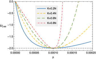
Figure 3: Plot of factor $\left.S\right|_{\text{std}}$ with respect to the a priori probability $p$ for the database model with two-value a priori probabilities. The number of database elements is $N=10^{4}$, and the number of elements with a priori probability $p$ is $K$. The factor $\left.S\right|_{\text{std}}$ is plotted for different $K$. Note that the range of $p$ varies with different $K$, as $Kp$ cannot exceed the total a priori probability $1$. It can be seen that all the lines have the minimum value $-2$ at the point $p=10^{-4}$, as this is the case of uniform a priori probabilities corresponding to the original Grover quantum search algorithm which is already optimal and cannot be optimized anymore. All the other points with $p\neq 10^{-4}$ represent the cases of nonuniform a priori probability distributions which can be optimized by the approach presented in this paper, and the smaller the factor $\left.S\right|_{\text{std}}$ is, the more the number of Grover iterations can be reduced.

An interesting special case is that the a priori probabilities for different elements of the database are uniform, i.e.,

$$p=\frac{1}{N},$$ (60)

which is exactly the case considered by the standard Grover search algorithm. It can be obtained from Eq. (58) as well as observed from Fig. 3 that for this case,

$$\left.S\right|_{\text{std}}=-2,$$ (61)

implying that the query complexity of the original Grover search algorithm can also be decreased if a failure probability of the search algorithm is allowed.

The above result $\left.S\right|_{\text{std}}=-2$ for the original Grover search algorithm can also be obtained in a straightforward way as follows, without invoking the method introduced in the previous section. As the success probability of the original Grover algorithm to find the solution of the search problem with $j$ steps of Grover iterations is known to be

$$P_{G}=\sin^{2}\left[\left(2j+1\right){\rm arccsc}\sqrt{N}\right]=\sin^{2}\left(\lambda+{\rm arccsc}\sqrt{N}\right),$$ (62)

where $P_{G}$ denotes the success probability for the original Grover search algorithm and $\lambda$ is the renormalized number of oracle calls defined in (24), one can obtain

$$\frac{dP_{G}}{d\lambda} =\sin\left(2\lambda+2{\rm arccsc}\sqrt{N}\right),$$ (63)

$$\frac{d^{2}P_{G}}{d\lambda^{2}} =2\cos\left(2\lambda+2{\rm arccsc}\sqrt{N}\right).$$

For the original Grover search algorithm,

$$P_{G}=1,\;\lambda=\frac{\pi}{2}-{\rm arccsc}\sqrt{N},$$ (64)

so, one can obtain that

$$\frac{dP_{G}}{d\lambda}=0,$$ (65)

which can be understood from that $P_{G}$ is at the maximal value $1$, and

$$\frac{d^{2}P_{G}}{d\lambda^{2}}=-2,$$ (66)

which is in accordance with the result $\left.S\right|_{\text{std}}=-2$ in Eq. (61).

This result for the original Grover search algorithm seems quite natural, as a failure probability of the search algorithm can certainly allow a reduction in the number of oracle calls. Also, note that the initial state of the system and the reflection axis of the diffusion operator are not optimized to obtain $\left.S\right|_{\text{std}}=-2$ in this case, since it can be verified that for the original Grover search algorithm, the uniformly superposed state (1) is already the optimal choice for the initial state and the reflection axis even when a failure probability of the search algorithm is allowed.

However, this is not the case when the a priori probabilities of the database elements are not uniform. For nonuniform a priori probabilities, one needs to change the initial state of the system and the reflection axis of the diffusion operator to minimize the query complexity of the quantum search algorithm, and this is the goal of the optimization method proposed in the previous section. In fact, by the optimization of the initial state and the reflection axis, the quantum search algorithm can gain more increase in the efficiency for database elements with nonuniform a priori probabilities than with uniform a priori probabilities. This can be observed from Fig. (3) as $\left.S\right|_{\text{std}}=-2$ of the original Grover search algorithm has the largest absolute value over all possible values of $\left.S\right|_{\text{std}}$ for various a priori probabilities $p$.

As Eq. (59) indicates that a smaller $S$ results in a larger decrease in the number of oracle calls, Fig. 3 and Eq. (59) imply that all nonuniform a priori probability distributions of the database elements have a bigger boost in the efficiency of the quantum search algorithm than the uniform a priori probability distribution for the original Grover quantum search algorithm. This shows the advantage of a nonuniform a priori distribution of database elements in optimizing the performance of quantum search algorithm, which is in accordance with the intuition that one may exploit nonuniform a priori probability distribution of database elements to adjust the initial state of the system and the reflection axis of the diffusion operator to be more beneficial to the states with higher a priori probabilities so that the quantum search algorithm can have lower query complexity on average.

As remarked in the preceding section, though the optimization of the quantum search algorithm relies on the decrease of the success probability which may require more trials of the algorithm to find the target, such an optimization approach can still increase the efficiency of the search algorithm on average, as the decrease of the success probability is of order $O(\Delta P)$ while the decrease of the number of oracle calls is of order $O(\sqrt{\Delta P})$, the latter of which is much larger when $\Delta P$ is small. The above result for the original quantum search algorithm with uniform a priori probabilities can serve as an intuitive example of this point. It can be seen from Eq. (62) that when the quantum search algorithm is close to completion, i.e., $\left(2j+1\right)\arcsin\frac{1}{\sqrt{n}}$ is close to $\frac{\pi}{2}$, the increase of the number of oracle calls $j$ can hardly increase the success probability, so if a negligible portion of success probability is dropped, a significant portion of oracle iterations may be reduced! This is why the query complexity of the original Grover search algorithm can be improved by the optimization method.

IV.2 Discussion

In the preceding subsection, we expanded the change of average success probability $d\bar{P}$ of the quantum search algorithm to the second order of $d\lambda$ which generates an approximate optimal solution to the number of iterations in terms of $d\bar{P}$.. As we expand $d\bar{P}$ to the lowest nonzero order, i.e., the second order, of $d\lambda$, it is intuitive that if $d\bar{P}$ becomes large, this approximation will break. So there exists an effective range of $d\bar{P}$ to validate the above approximate optimal solution.

In this subsection, we investigate the effectiveness of the above approximate optimal solution by using the first-order optimal initial state and reflection axis and expanding $d\bar{P}$ to the third-order of $d\lambda$ to generate a more accurate optimal solution of the renormalized iteration number. The deviation of this more accurate optimal solution from that in the last subsection will give the effective range of $d\bar{P}$.

As the approximate optimal solution is obtained in the vicinity of $\bar{P}=1$ which is the maximal value of $\bar{P}$, the first-order term in the expansion of $d\bar{P}$ must be zero, so the expansion always starts from the second order of $d\lambda$. We plug the approximate optimal solution to the initial state $|\psi\rangle$ and the reflection axis $|\varphi\rangle$ of diffusion (100) (in terms of $|d\psi\rangle$ and $|d\varphi\rangle$) into the average success probability $\bar{P}$ (25), and expand the change of the success probability to the third order of $d\lambda$,

$$d\bar{P}=\frac{1}{2}Sd\lambda^{2}+\frac{1}{6}Gd\lambda^{3}.$$ (67)

From this expansion, one can work out $d\lambda$ in terms of $d\bar{P}$,

$$d\lambda=-\sqrt{\frac{2d\bar{P}}{\left.S\right|_{\text{std}}}}+\left.B\right|_{\text{std}}d\bar{P},$$ (68)

with $\left.S\right|_{\text{std}}$ obtained in Eq. (58) and

$$\left.B\right|_{\text{std}}=-\frac{(K-1)K(N-2)(Np-1)^{2}{\rm arccsc}\sqrt{N}}{\pi\sqrt{N-1}Np(-2KNp+K+Np)(KNp-1)}$$ . (69)

The mathematical details of the derivation can be found in Appendix D.

Eq. (68) is an extension of the result in the last subsection to involve the first order of $d\bar{P}$. To validate the approximation, this additional term should be much smaller than the term of order $\frac{1}{2}$, so it leads to the effective range of $d\bar{P}$ for the approximation,

$$d\bar{P}\ll\frac{2}{\left.S\right|_{\text{std}}(\left.B\right|_{\text{std}})^{2}}.$$ (70)

What if $S$ is too small, say $S\ll B$? For example, one can see from Fig. 3 that $S$ approaches zero when the a priori probability of some database elements is zero, i.e., $p=0$. This seems peculiar at first glance, but is actually in accordance with physics. Note that the portion of database elements with a priori probability $p=0$ can never be a solution of the quantum search task, so the quantum search algorithm can be restricted to the remaining part of the database which includes $N-K$ elements in this case, which can immediately reduce the query complexity of the quantum search algorithm from $O(\sqrt{N})$ to $O(\sqrt{N-K})$, even without a drop of the success probability! This means that we can have a nonzero $d\lambda$ when $d\bar{P}=0$ for this case, which leads to $S=d\bar{P}/d\lambda^{2}=0$.

However, it should also be noted that when $S$ is too small, the second-order approximation for the expansion of $d\bar{P}$ is no longer sufficient, and one must keep higher-order terms in Eq. (67) to derive $d\lambda$. The solution to $d\lambda$ for this case can be much more complex than that with the second-order approximation, but is still tractable as Eq. (67) is always a polynomial equation in essence.

To illustrate the effect of higher order terms on the approximation, the exact ratio of the change $d\bar{P}$ in the average success probability to the square of the change $d\lambda$ in the renormalized number of iteration steps is plotted in Fig. 4 for different $p$ and $K$, which shows the deviation of $d\bar{P}/d\lambda^{2}$ from $\left.S\right|_{\text{std}}$ when $|d\bar{P}|$ becomes large and thus the necessity to include higher-order terms of $d\lambda$ in the expansion of $d\bar{P}$ for this case as shown in Eq. (67).

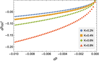
(a)

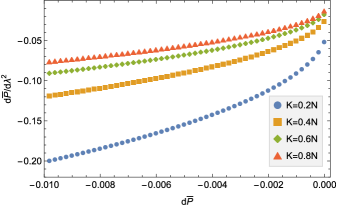
(b)

Figure 4: Plots of the exact ratio of the change $d\bar{P}$ in the average success probability to the square of the change $d\lambda$ in the renormalized iteration steps for a database with different two-value a priori probability distributions: (a) $p=\left(1-10^{-6}\right)/K$ and (b) $p=10^{-6}$. The number of database elements is $N=10^{4}$, and the number of elements with a priori probability $p$ is $K$. Lines with different colors indicate different choices of $K$. The plots show how $d\bar{P}/d\lambda^{2}$ deviates from $\left.S\right|_{\text{std}}$ when $|d\bar{P}|$ becomes large and thus the necessity to keep higher-order terms of $d\lambda$ in the expansion of $d\bar{P}$ for this scenario as shown in Eq. (67).

V Conclusions

In this work, we studied the quantum search algorithm with general a priori probabilities for the elements of the database to be the solution of the search problem, and optimized the initial state of the quantum system and the reflection axis of the diffusion operator by a variational approach to minimize the number of oracle calls at the expense of a failure probability of the quantum search algorithm. We obtained the optimization conditions for the initial state and the reflection axis, but the optimization equations are difficult to solve due to being highly nonlinear, so we assumed the failure probability of the quantum search algorithm to be low so that the optimized initial state and reflection axis have just slight deviations from those in the standard Grover search algorithm and thus a differentiation approach can be exploited to obtain the differential relation between the initial state of the quantum system, the reflection axis of the diffusion operator, the renormalized number of Grover iterations and the success probability of the search algorithm. We obtained a formal approximate solution to the renormalized number of oracle calls in terms of the decrease in the success probability, and applied it to a simple database model with two-value a priori probabilities of the elements to exemplify the power of the optimization results. The results showed that the optimization can indeed lower the query complexity of the quantum search algorithm, even for the original Grover search algorithm with uniform a priori probabilities for the database elements, which is not surprising as the success probability of the search algorithm is lowered, but the optimization can lead to a larger reduction in the query complexity when the a priori probability distribution is nonuniform, which suggests the advantage of nonuniform a priori probability distributions in improving the efficiency of the quantum search algorithm.

We remark that the current results are effective for a small failure probability, as we expanded the success probability only to the lowest-order nonzero differential of the renormalized number of oracle calls. If one wants to obtain results effective for larger failure probabilities, higher-order differentials of the renormalized number of oracle calls need to be included. The way to expand the success probability to higher-order differentials of the renormalized number of oracle calls is similar to the differentiation approach presented in this work. The main difference lies in that the differential equation (49) will include multiple higher-order terms of the renormalized number of oracle calls, so one will need to solve a polynomial equation to obtain the solution for the decrease of the renormalized number of oracle calls, which will increase the complexity of this optimization problem if one wants to find analytical results but can be solved efficiently by numerical computation.

We hope this work can provide a new perspective on the quantum search problem, and stimulate further research in improving the efficiency of quantum search algorithm by a priori information.

Appendix A Variation of success probability for generalized quantum search algorithm

In combination with the prior distribution, the final success probability $\bar{P}$ can be written as

$$\bar{P}=\sum_{t}p_{t}\langle\psi|P_{t}|\psi\rangle\sin^{2}\left(\lambda\frac{\arcsin\langle t\lvert\varphi\rangle}{{\rm arccsc}\sqrt{N}}+\arcsin\frac{\langle t|P_{t}|\psi\rangle}{\sqrt{\langle\psi|P_{t}|\psi\rangle}}\right)$$ (71)

where $\lambda=2j{\rm arccsc}\sqrt{N}$.

The variation of $\bar{P}$ can be written as

$$\delta\bar{P}=\langle\delta\psi|a_{\psi}\rangle+\langle\delta\varphi|b_{\varphi}\rangle+c_{\lambda}\delta\lambda.$$ (72)

The unnormalized states $|a_{\psi}\rangle$ can be obtained by taking the variation of $\bar{P}$ (71) with respect to $|\psi\rangle$, which turns out to be

$$|\text{$a_{\psi}\rangle=$} \sum_{t}p_{t}\frac{\sqrt{1-b_{t}^{2}}(2a_{t}b_{t}-c)\sin\frac{2\lambda\arcsin b_{t}}{{\rm arccsc}\sqrt{N}}+\left[a_{t}\left(2b_{t}^{2}-1\right)-\text{$b_{t}$}c\right]\cos\frac{2\lambda\arcsin\text{$b_{t}$}}{{\rm arccsc}\sqrt{N}}-\text{$a_{t}$}+\text{$b_{t}$}c}{b_{t}^{2}-1}\lvert t\rangle$$ (73)

$$+\sum_{t}p_{t}\frac{-a_{t}\sqrt{1-\text{$b_{t}$}^{2}}\sin\frac{2\lambda\arcsin\text{$b_{t}$}}{{\rm arccsc}\sqrt{N}}+(c-\text{$a_{t}$}b_{t})\cos\frac{2\lambda\arcsin b_{t}}{{\rm arccsc}\sqrt{N}}+a_{t}\text{$b_{t}$}-c}{\text{$b_{t}$}^{2}-1}\lvert\varphi\rangle,$$

where

$$a_{t}=\langle t|\psi\rangle,\;b_{t}=\langle t|\varphi\rangle,\;c=\langle\varphi|\psi\rangle.$$ (74)

Similarly, the unnormalized state $|\text{$b_{\varphi}\rangle$}$ can be obtained as

$$|\text{$b_{\varphi}\rangle=$} \sum_{t}\frac{p_{t}}{\left(b_{t}^{2}-1\right)^{2}}\left\{\frac{\lambda\left\{\sqrt{1-\text{$b_{t}$}^{2}}\left[\text{$a_{t}$}^{2}\left(2\text{$b_{t}$}^{2}-1\right)-2\text{$a_{t}$}\text{$b_{t}$}c+c^{2}\right]\sin\frac{2\lambda\arcsin\text{$b_{t}$}}{\csc^{-1}\sqrt{n}}+2\text{$a_{t}$}\left(b_{t}^{2}-1\right)(a_{t}\text{$b_{t}$}-c)\cos\frac{2\lambda\arcsin b_{t}}{{\rm arccsc}\sqrt{N}}\right\}}{{\rm arccsc}\sqrt{N}}\right.$$ (75)

$$\left.-(a_{t}-\text{$b_{t}$}c)\left[a_{t}\sqrt{1-b_{t}^{2}}\sin\frac{2\lambda\arcsin b_{t}}{{\rm arccsc}\sqrt{N}}+(\text{$a_{t}$}\text{$b_{t}$}-c)\cos\frac{2\lambda\arcsin b_{t}}{{\rm arccsc}\sqrt{N}}-a_{t}b_{t}+c\right]\right\}\lvert t\rangle$$

$$+\sum_{t}p_{t}\frac{\text{$a_{t}$}\sqrt{1-\text{$b_{t}$}^{2}}\sin\frac{2\lambda\arcsin b_{t}}{{\rm arccsc}\sqrt{N}}+(\text{$a_{t}$}b_{t}-c)\cos\frac{2\lambda\arcsin b_{t}}{{\rm arccsc}\sqrt{N}}-\text{$a_{t}$}b_{t}+c}{1-b_{t}^{2}}\lvert\psi\rangle,$$

and the coefficient $c_{\lambda}$ can be obtained as

$$c_{\lambda}=\sum_{t}p_{t}\arcsin\text{{\hbox{b_{t}}}}\frac{\left[\text{\text{{\hbox{a_{t}}}}}^{2}\left(1-2\text{{\hbox{b_{t}}}}^{2}\right)+2\text{{\hbox{a_{t}}}}\text{{\hbox{b_{t}}}}c-c^{2}\right]\sin\frac{2\lambda\arcsin\text{{\hbox{b_{t}}}}}{{\rm arccsc}\sqrt{N}}+2\text{{\hbox{a_{t}}}}\sqrt{1-\text{{\hbox{b_{t}}}}^{2}}(\text{\text{{\hbox{a_{t}}}}}\text{{\hbox{b_{t}}}}-c)\cos\frac{2\lambda\arcsin b_{t}}{{\rm arccsc}\sqrt{N}}}{\left(\text{\text{{\hbox{b_{t}}}}}^{2}-1\right){\rm arccsc}\sqrt{N}}$$ (76)

The differentials of $|a_{\psi}\rangle$, $|\text{$b_{\varphi}\rangle$}$ in Eq. (33), (37) can be straightforwardly obtained by taking differentiation of (73) and (75), which are not presented here as they are quite lengthy.

Appendix B Derivation of submatrices in $M$ and $T$ with parameters of original Grover algorithm

In this appendix, we derive the matrices and vectors involved in the computation in Sec. III.3, particularly the submatrices of $M$ (41) and $T$ (44), i.e., $A_{\psi\psi}$, $A_{\psi\varphi}$, $B_{\varphi\psi}$, $B_{\varphi\varphi}$ and $\widetilde{A_{\psi}}$, $\widetilde{A_{\varphi}}$, $\widetilde{B_{\psi}},\widetilde{B_{\varphi}}$, with the parameters of the standard Grover search algorithm, so that the differentials of $|\psi\rangle$, $|\varphi\rangle$ and $\lambda$ represent the deviation from those in the standard Grover search algorithm.

By invoking the standard Grover quantum search algorithm and using the results of $|a_{\psi}\rangle$, $|b_{\varphi}\rangle$ and $\lambda$ in Appendix A, it can be obtained that

$$\left.|a_{\psi}\rangle\right|_{\text{std}}=\left.|b_{\varphi}\rangle\right|_{\text{std}}=2|\psi_{0}\rangle,\;\left.c_{\lambda}\right|_{\text{std}}=0,$$ (77)

where the subscript “std” indicates the terms are evaluated with $|\psi\rangle$, $|\varphi\rangle$ and $\lambda$ given by the standard Grover search algorithm, i.e.,

$$\left.|\psi\rangle\right|_{\text{std}}=\left.|\varphi\rangle\right|_{\text{std}}=|\psi_{0}\rangle,\;\left.\lambda\right|_{\text{std}}=\frac{\pi}{2}-{\rm arccsc}\sqrt{N},$$ (78)

where $|\psi_{0}\rangle$ is the uniformly superposed state defined in Eq. (1).

Taking the differentiation of $|a_{\psi}\rangle$, $|b_{\varphi}\rangle$, $\lambda$ in Appendix A and evaluating the resulting differentials with $|\psi\rangle$, $|\varphi\rangle$ and $\lambda$ from the standard Grover search algorithm, one obtains

$$|da_{\psi}\rangle =\left.A_{\psi\psi}\right|_{\text{std}}|d\psi\rangle+\left.A_{\psi\varphi}\right|_{\text{std}}|d\varphi\rangle+\left.|a_{\psi\lambda}\rangle\right|_{\text{std}}d\lambda,$$ (79)

$$|db_{\varphi}\rangle =\left.B_{\varphi\psi}\right|_{\text{std}}|d\psi\rangle+\left.B_{\varphi\varphi}\right|_{\text{std}}|d\varphi\rangle+\left.|b_{\varphi\lambda}\rangle\right|_{\text{std}}d\lambda,$$

where

$$\left.A_{\psi\psi}\right|_{\text{std}} =2|\psi_{0}\rangle\langle\psi_{0}|,$$ (80)

$$\left.A_{\psi\varphi}\right|_{\text{std}} =2\left(I+|\psi_{0}\rangle\langle\psi_{0}|\right)+\frac{\pi\sqrt{N}|\psi_{0}\rangle\langle\eta|-\pi N\sum_{t}p_{t}|t\rangle\langle t|}{(N-1){\rm arccsc}\sqrt{N}},$$

$$\left.|a_{\psi\lambda}\rangle\right|_{\text{std}} =\frac{2|\psi_{0}\rangle-2\sqrt{N}|\eta\rangle}{\sqrt{N-1}},$$

$$\left.B_{\varphi\psi}\right|_{\text{std}} =2\left(I+|\psi_{0}\rangle\langle\psi_{0}|\right)+\frac{\pi\sqrt{N}|\eta\rangle\langle\psi_{0}|-\pi N\sum_{t}p_{t}|t\rangle\langle t|}{(N-1){\rm arccsc}\sqrt{N}},$$ (81)

$$\left.B_{\varphi\varphi}\right|_{\text{std}} =\frac{\pi N\left(\pi-4{\rm arcsec}\sqrt{N}\right)\sum_{t}p_{t}|t\rangle\langle t|}{2(N-1){\rm arccsc}^{2}\sqrt{N}}+\frac{\pi\sqrt{N}\left(|\psi_{0}\rangle\langle\eta|+|\eta\rangle\langle\psi_{0}|\right)}{(N-1){\rm arccsc}\sqrt{n}}+2|\psi_{0}\rangle\langle\psi_{0}|,$$

$$\left.|b_{\varphi\lambda}\rangle\right|_{\text{std}} =\frac{2|\psi_{0}\rangle+2\sqrt{N}|\eta\rangle}{\sqrt{N-1}}-\frac{\sqrt{N}\pi|\eta\rangle}{\sqrt{N-1}{\rm arccsc}\sqrt{N}},$$

and

$$|\eta\rangle=\sum_{t}p_{t}|t\rangle,$$ (82)

which is an unnormalized state determined by the a priori probability distribution $p_{t}$ of the database elements. With the above $\left.A_{\psi\psi}\right|_{\text{std}}$, $\left.A_{\psi\varphi}\right|_{\text{std}}$, $\left.B_{\varphi\psi}\right|_{\text{std}}$, $\left.B_{\varphi\varphi}\right|_{\text{std}}$, one can obtain the matrix $T$ for $|da_{\psi}\rangle$ and $|db_{\varphi}\rangle$ (43).

The matrices $\widetilde{A_{\psi}}$, $\widetilde{A_{\varphi}}$, $\widetilde{B_{\psi}}$, $\widetilde{B_{\varphi}}$ can be also be obtained accordingly by using the definitions (36) and (39) as

$$\left.\widetilde{A_{\psi}}\right|_{\text{std}} =2I,$$ (83)

$$\left.\widetilde{A_{\varphi}}\right|_{\text{std}} =2\left(|\psi_{0}\rangle\langle\psi_{0}|-I\right)+\frac{\pi N\sum_{t}p_{t}|t\rangle\langle t|-\pi\sqrt{N}|\psi_{0}\rangle\langle\eta|}{(N-1){\rm arccsc}\sqrt{N}},$$

$$\left.\widetilde{B_{\psi}}\right|_{\text{std}} =-2I+\frac{\pi N\sum_{t}p_{t}|t\rangle\langle t|-\pi\sqrt{N}\left(|\psi_{0}\rangle\langle\eta|+|\eta\rangle\langle\psi_{0}|\right)+\pi+2\pi(N-1){\rm arccsc}\sqrt{N}|\psi_{0}\rangle\langle\psi_{0}|}{(N-1){\rm arccsc}\sqrt{N}},$$

$$\left.\widetilde{B_{\varphi}}\right|_{\text{std}} =2I+\frac{\pi\left(|\psi_{0}\rangle\langle\psi_{0}|-\sqrt{N}|\eta\rangle\langle\psi_{0}|\right)}{(N-1){\rm arccsc}\sqrt{N}}+\frac{\pi\left(\pi-4{\rm arccsc}\sqrt{N}\right)}{2(N-1){\rm arccsc}^{2}\sqrt{N}}\left(N\sum_{t}p_{t}|t\rangle\langle t|-\sqrt{N}|\psi_{0}\rangle\langle\eta|\right).$$

With $\left.\widetilde{A_{\psi}}\right|_{\text{std}}$, $\left.\widetilde{A_{\varphi}}\right|_{\text{std}}$, $\left.\widetilde{B_{\psi}}\right|_{\text{std}}$ and $\left.\widetilde{B_{\varphi}}\right|_{\text{std}}$, one can obtain the matrix $M$ for $|d\psi\rangle$ and $|d\varphi\rangle$ (42).

In addition, the differential of $c_{\lambda}$ can also be obtained with the parameters from the standard Grover quantum search algorithm,

$$\left.dc_{\lambda}\right|_{\text{std}}=-2\left(\frac{\sqrt{N}{\rm arcsec}\sqrt{N}\langle\eta|d\varphi\rangle}{\sqrt{N-1}{\rm arccsc}\sqrt{N}}+\frac{\sqrt{N}\langle\eta|d\psi\rangle}{\sqrt{N-1}}+d\lambda\right),$$ (84)

and the vectors $|v_{a}\rangle$, $|v_{b}\rangle$ in Eqs. (36) and (39) can be obtained as

$$\left.|v_{a}\rangle\right|_{\text{std}}=\frac{2|\psi_{0}\rangle-2\sqrt{N}|\eta\rangle}{\sqrt{N-1}}d\lambda,\;\left.|v_{b}\rangle\right|_{\text{std}}=\frac{{\rm arcsec}\sqrt{N}}{{\rm arccsc}\sqrt{N}}|v_{a}\rangle.$$ (85)

Appendix C Derivation of the results for database with two-value a priori probabilities

In this appendix, we provide the mathematical details of the derivation of the results for the database with two-value a priori probabilities in Sec. IV.

Consider a database of $N$ elements, the a priori probabilities of which to be the search target are two valued. For example, there are $K$ elements in the database with a priori probabilities $p$ to be the search target and the other $N-K$ elements with a priori probabilities $q$ to be the search target,

$$q=\frac{1-Kp}{N-K}.$$ (86)

We use the method introduced in Appendix B to optimize the quantum search algorithm for this database model given a small failure probability. The variation of the average success probability with respect to the initial state $|\psi\rangle$, the reflection axis $|\varphi\rangle$ of the diffusion operator and the renormalized number $\lambda$ of oracle calls produces $|a_{\psi}\rangle$, $|b_{\varphi}\rangle$, and $c_{\lambda}$ respectively, according to Eq. (26),

$$\left.|a_{\psi}\rangle\right|_{\text{std}} =\frac{2}{\sqrt{N}}E_{N\times 1},$$ (87)

$$\left.|b_{\varphi}\rangle\right|_{\text{std}} =\frac{2}{\sqrt{N}}E_{N\times 1},$$ (88)

$$\left.c_{\lambda}\right|_{\text{std}} =0,$$ (89)

with $|\psi\rangle$, $|\varphi\rangle$ and $\lambda$ given by the standard Grover search algorithm, and $E_{n\times m}$ an $n\times m$ matrix defined as

$$E_{n\times m}=\underset{m\,\mathrm{columns}}{\left.\underbrace{\begin{bmatrix}1&1&\cdots&1\\ 1&1&\cdots&1\\ \vdots&\vdots&\ddots&\vdots\\ 1&1&\cdots&1\end{bmatrix}}\right\}}n\,\mathrm{rows}$$ (90)

So, $E_{N\times 1}$ is just an $N$-dimensional vector with all the elements being 1’s. For the sake of simplicity, we will also denote $E_{k\times k}$ by $E_{k}$ in the following.

Taking the differentiation of $|a_{\psi}\rangle$, $|b_{\varphi}\rangle$, and $c_{\lambda}$ with the parameters from the standard Grover search algorithm, one can work out that

$$\left.|da_{\psi}\rangle\right|_{\text{std}} =\left.A_{\psi\psi}\right|_{\text{std}}|d\varphi\rangle+\left.A_{\psi\varphi}\right|_{\text{std}}|d\varphi\rangle+\left.|a_{\psi\lambda}\rangle\right|_{\text{std}}d\lambda,$$ (91)

$$\left.|db_{\varphi}\rangle\right|_{\text{std}} =\left.B_{\varphi\psi}\right|_{\text{std}}|d\psi\rangle+\left.B_{\varphi\varphi}\right|_{\text{std}}|d\varphi\rangle+\left.|b_{\varphi\lambda}\rangle\right|_{\text{std}}d\lambda,$$

where

$$\left.A_{\psi\psi}\right|_{\text{std}} =\frac{2}{N}E_{N},$$ (92)

$$\left.A_{\psi\varphi}\right|_{\text{std}} =\begin{bmatrix}2(I_{K}+E_{K})+\frac{\pi p}{(N-1){\rm arccsc}\sqrt{N}}\left(-NI_{K}+E_{K}\right)&\left[2+\frac{\pi q}{(N-1){\rm arccsc}\sqrt{N}}\right]E_{K\times(N-K)}\\ \left[2+\frac{\pi p}{(N-1){\rm arccsc}\sqrt{N}}\right]E_{(N-K)\times K}&2(I_{N-K}+E_{N-K})+\frac{\pi q}{(N-1){\rm arccsc}\sqrt{N}}\left(-NI_{N-K}+E_{N-K}\right)\end{bmatrix},$$

$$\left.|a_{\psi\lambda}\rangle\right|_{\text{std}} =\begin{bmatrix}\left(\frac{2}{\sqrt{N\left(N-1\right)}}-\frac{2\sqrt{N}p}{\sqrt{N-1}}\right)E_{K\times 1}\\ \left(\frac{2}{\sqrt{N\left(N-1\right)}}-\frac{2\sqrt{N}q}{\sqrt{N-1}}\right)E_{(N-K)\times 1}\end{bmatrix},$$

and

$$\left.B_{\varphi\psi}\right|_{\text{std}} =\begin{bmatrix}2(I_{K}+E_{K})+\frac{\pi p}{(N-1){\rm arccsc}\sqrt{N}}\left(-NI_{K}+E_{K}\right)&\left[2+\frac{\pi p}{(N-1){\rm arccsc}\sqrt{N}}\right]E_{K\times(N-K)}\\ \left[2+\frac{\pi q}{(N-1){\rm arccsc}\sqrt{N}}\right]E_{(N-K)\times K}&2(I_{N-K}+E_{N-K})+\frac{\pi q}{(N-1){\rm arccsc}\sqrt{N}}\left(-NI_{N-K}+E_{N-K}\right)\end{bmatrix},$$ (93)

$$\left.B_{\varphi\varphi}\right|_{\text{std}} =\begin{bmatrix}\frac{\pi p\left(\pi-4{\rm arccsc}\sqrt{N}\right)N}{2(N-1){\rm arccsc}^{2}\sqrt{N}}I_{K}+\left[2+\frac{2\pi p}{(N-1){\rm arccsc}\sqrt{N}}\right]E_{K}&\left[2+\frac{\pi(p+q)}{(N-1){\rm arccsc}\sqrt{N}}\right]E_{K\times(N-K)}\\ \left[2+\frac{\pi(p+q)}{(N-1){\rm arccsc}\sqrt{N}}\right]E_{(N-K)\times K}&\frac{\pi q\left(\pi-4{\rm arccsc}\sqrt{N}\right)N}{2(N-1){\rm arccsc}^{2}\sqrt{N}}I_{N-K}+\left[2+\frac{2\pi q}{(N-1){\rm arccsc}\sqrt{N}}\right]E_{N-K}\end{bmatrix},$$

$$\left.|b_{\varphi\lambda}\rangle\right|_{\text{std}} =\begin{bmatrix}\left(\frac{2}{\sqrt{N\left(N-1\right)}}+\frac{2\sqrt{N}p}{\sqrt{N-1}}-\frac{\sqrt{N}\pi p}{\sqrt{N-1}{\rm arccsc}\sqrt{N}}\right)E_{K\times 1}\\ \left(\frac{2}{\sqrt{N\left(N-1\right)}}+\frac{2\sqrt{N}q}{\sqrt{N-1}}-\frac{\sqrt{N}\pi q}{\sqrt{N-1}{\rm arccsc}\sqrt{N}}\right)E_{(N-K)\times 1}\end{bmatrix}.$$

With $\left.A_{\psi\psi}\right|_{\text{std}}$, $\left.A_{\psi\varphi}\right|_{\text{std}}$, $\left.B_{\varphi\psi}\right|_{\text{std}}$, $\left.B_{\varphi\varphi}\right|_{\text{std}}$, one can obtain the matrix $T$ that is necessary for the derivation of $|da_{\psi}\rangle$ and $|db_{\varphi}\rangle$ in (43).

The four block submatrices $\widetilde{A_{\psi}}$, $\widetilde{A_{\varphi}}$, $\widetilde{B_{\psi}}$, $\widetilde{B_{\varphi}}$ for the matrix $M$ in (41) can be also obtained with the parameters from the standard quantum search algorithm as

$$\left.\widetilde{A_{\psi}}\right|_{\text{std}} =2I_{N},$$ (94)

$$\left.\widetilde{A_{\varphi}}\right|_{\text{std}} =\begin{bmatrix}\left[\frac{2}{N}-\frac{\pi p}{(N-1){\rm arccsc}\sqrt{N}}\right]\left(E_{K}-NI_{K}\right)&\left[\frac{2}{N}-\frac{\pi q}{(N-1){\rm arccsc}\sqrt{N}}\right]E_{K\times(N-K)}\\ \left[\frac{2}{N}-\frac{\pi p}{(N-1){\rm arccsc}\sqrt{N}}\right]E_{(N-K)\times K}&\left[\frac{2}{N}-\frac{\pi q}{(N-1){\rm arccsc}\sqrt{N}}\right]\left(E_{N-K}-NI_{N-K}\right)\end{bmatrix},$$

$$\left.\widetilde{B_{\psi}}\right|_{\text{std}} =\begin{bmatrix}-2I_{K}+\frac{\pi+2\pi(N-1){\rm arccsc}\sqrt{N}E_{K}}{N(N-1){\rm arccsc}\sqrt{N}}+\frac{\pi p\left(NI_{K}-2E_{K}\right)}{(N-1){\rm arccsc}\sqrt{N}}&\left[\frac{\pi+2\pi(N-1){\rm arccsc}\sqrt{N}}{N(N-1){\rm arccsc}\sqrt{N}}-\frac{\pi(p+q)}{(N-1){\rm arccsc}\sqrt{N}}\right]E_{K\times(N-K)}\\ \left[\frac{\pi+2\pi(N-1){\rm arccsc}\sqrt{N}}{N(N-1){\rm arccsc}\sqrt{N}}-\frac{\pi(p+q)}{(N-1){\rm arccsc}\sqrt{N}}\right]E_{(N-K)\times K}&-2I_{N-K}+\frac{\pi+2\pi(N-1){\rm arccsc}\sqrt{N}E_{N-K}}{N(N-1){\rm arccsc}\sqrt{N}}+\frac{\pi q\left(NI_{N-K}-E_{N-K}\right)}{(N-1){\rm arccsc}\sqrt{N}}\end{bmatrix}$$

$$\left.\widetilde{B_{\varphi}}\right|_{\text{std}} =\begin{bmatrix}2I_{K}+\frac{\pi\left(\frac{1}{N}-p\right)E_{K}}{(N-1){\rm arccsc}\sqrt{N}}+\frac{\pi p\left(\pi-4{\rm arccsc}\sqrt{N}\right)\left(NI_{K}-E_{K}\right)}{2(N-1){\rm arccsc}^{2}\sqrt{N}}&\left[\frac{\pi\left(\frac{1}{N}-p\right)}{(N-1){\rm arccsc}\sqrt{N}}-\frac{\pi q\left(\pi-4{\rm arccsc}\sqrt{N}\right)}{2(N-1){\rm arccsc}^{2}\sqrt{N}}\right]E_{K\times(N-K)}\\ \left[\frac{\pi\left(\frac{1}{N}-q\right)}{(N-1){\rm arccsc}\sqrt{N}}-\frac{\pi p\left(\pi-4{\rm arccsc}\sqrt{N}\right)}{2(N-1){\rm arccsc}^{2}\sqrt{N}}\right]E_{(N-K)\times K}&2I_{N-K}+\frac{\pi\left(\frac{1}{N}-q\right)E_{N-K}}{(N-1){\rm arccsc}\sqrt{N}}+\frac{\pi q\left(\pi-4{\rm arccsc}\sqrt{N}\right)\left(NI_{N-K}-E_{N-K}\right)}{2(N-1){\rm arccsc}^{2}\sqrt{N}}\end{bmatrix}$$

With $\left.\widetilde{A_{\psi}}\right|_{\text{std}}$, $\left.\widetilde{A_{\varphi}}\right|_{\text{std}}$, $\left.\widetilde{B_{\psi}}\right|_{\text{std}}$ and $\left.\widetilde{B_{\varphi}}\right|_{\text{std}}$, one can obtain the matrix $M$ and its inverse that is necessary for the derivation of $|d\psi\rangle$ and $|d\varphi\rangle$ in (42).

According to the above results, the inverse of the matrix $M$ can be found as

$$M^{-1}=\begin{bmatrix}\alpha_{1}(p)I_{K}+\beta_{1}(p,q)E_{K}&\gamma_{1}E_{K\times(N-K)}&\alpha_{2}(p)I_{K}+\beta_{2}(p,q)E_{K}&\gamma_{2}(p,q)E_{K\times(N-K)}\\ \gamma_{1}E_{(N-K)\times K}&\alpha_{1}(q)I_{N-K}+\beta_{1}(q,p)E_{N-K}&\gamma_{2}(q,p)E_{(N-K)\times K}&\alpha_{2}(q)I_{N-K}+\beta_{2}(q,p)E_{N-K}\\ \alpha_{3}(p)I_{K}+\beta_{3}(p)E_{K}&\gamma_{3}E_{K\times(N-K)}&\alpha_{4}(p)I_{K}+\beta_{4}(p,q)E_{K}&\gamma_{4}(p,q)E_{K\times(N-K)}\\ \gamma_{3}E_{(N-K)\times K}&\alpha_{3}(q)I_{N-K}+\beta_{3}(q)E_{N-K}&\gamma_{4}(q,p)E_{(N-K)\times K}&\alpha_{4}(q)I_{N-K}+\beta_{4}(q,p)E_{N-K}\end{bmatrix},$$ (95)

where the coefficients $\alpha_{i}$, $\beta_{i}$, $\gamma_{i}$, $i=1,2,3,4$, are functions defined as follows,

$$\alpha_{1}(x)= -\frac{(N-1)\left[\pi^{2}Nx-4\pi Nx{\rm arccsc}\sqrt{N}+4(N-1){\rm arccsc}^{2}\sqrt{N}\right]}{2\pi^{2}Nx\left[N(x-1)+1\right]},$$ (96)

$$\beta_{1}(x,y)= \frac{1}{2\pi^{2}N^{2}x\left[N(x-1)+1\right](p+q-1)\left[N(p+q)-1\right]}$$

$$\times\left\{-4(N-1)^{2}{\rm arccsc}^{2}\sqrt{N}\left(Nx^{2}-Npq+x-Ny^{2}+Ny\right)\right.$$

$$-4(N-1){\rm arccsc}\sqrt{N}\pi x\left[N(y-1)+1\right]\left[N(p+q)-1\right]$$

$$+\left.\pi^{2}x\left[N(p+q)-1\right]\left[N\left(Nx^{2}+Npq-2Nx+x+1\right)-1\right]\right\},$$

$$\gamma_{1}= \frac{\left\{\pi\left[N(p+q)-1\right]-2(N-1){\rm arccsc}\sqrt{N}\right\}^{2}}{2\pi^{2}N^{2}(p+q-1)\left[N(p+q)-1\right]},$$

$$\alpha_{2}(x)= \frac{(N-1){\rm arccsc}\sqrt{N}\left[\pi Nx-2(N-1){\rm arccsc}\sqrt{N}\right]}{\pi^{2}Nx\left[N(x-1)+1\right]},$$ (97)

$$\beta_{2}(x,y)= \frac{1}{2\pi^{2}N^{2}x\left[N(x-1)+1\right](p+q-1)\left[N(p+q)-1\right]}$$

$$\times\left\{-\pi x\left[N\left(2Nx^{2}+Npq-3Nx+Ny^{2}-Ny+x+3\right)-3\right]\right.$$

$$-4(N-1)^{2}{\rm arccsc}^{2}\sqrt{N}\left(Nx^{2}-Npq+x-Ny^{2}+Ny\right)$$

$$\left.+\pi^{2}x\left[N(x-1)+1\right](Nx-1)\left[N(p+q+1)-2\right]\right\},$$

$$\gamma_{2}(x,y)= \frac{\pi^{2}(Nx-1)\left[N(p+q+1)-2\right]+2(N-1){\rm arccsc}\sqrt{N}\left[3\pi-\pi N(3x+y)+2(N-1){\rm arccsc}\sqrt{N}\right]}{2\pi^{2}N^{2}(p+q-1)\left[N(p+q)-1\right]},$$

$$\begin{aligned} \alpha_{3}(x)=&\frac{(N-1){\rm arccsc}\sqrt{N}\left[\pi Nx-2(N-1){\rm arccsc}\sqrt{N}\right]}{\pi^{2}Nx\left[N(x-1)+1\right]},\\ \beta_{3}(x,y)=&\frac{-(N-1){\rm arccsc}\sqrt{N}}{\pi^{2}N^{2}p\left[N(x-1)+1\right]\left[N(p+q)-1\right](p+q-1)}\\ &\times\left\{\pi x\left[N(y-1)+1\right]\left[N(p+q)-1\right]+2(N-1){\rm arccsc}\sqrt{N}\left(Nx^{2}-Npq-x-Ny^{2}+Ny\right)\right\},\\ \gamma_{3}=&\frac{(N-1){\rm arccsc}\sqrt{N}\left[-\pi N(p+q)+2(N-1){\rm arccsc}\sqrt{N}+\pi\right]}{\pi^{2}N^{2}(p+q-1)\left[N(p+q)-1\right]},\end{aligned}$$ (98)

$$\begin{aligned} \alpha_{4}(x)=&-\frac{2(N-1)^{2}{\rm arccsc}^{2}\sqrt{N}}{\pi^{2}Nx\left[N(x-1)+1\right]},\\ \beta_{4}(x,y)=&\frac{-4(N-1){\rm arccsc}\sqrt{N}\left\{(N-1){\rm arccsc}\sqrt{N}\left(Nx^{2}-Npq-x-Ny^{2}+Ny\right)+\pi x\left[N(x-1)+1\right](Nx-1)\right\}}{2\pi^{2}N^{2}x\left[N(x-1)+1\right]\left[N(p+q)-1\right](p+q-1)}\\ &+\frac{y}{2\left[N(p+q)-1\right]},\\ \gamma_{4}(x,y)=&\frac{4(N-1){\rm arccsc}\sqrt{N}\left[-\pi Nx+(N-1){\rm arccsc}\sqrt{N}+\pi\right]}{2\pi^{2}N^{2}(p+q-1)\left[N(p+q)-1\right]}+\frac{y}{2\left[N(p+q)-1\right]}.\end{aligned}$$ (99)

According to the above results and Eq (42), the differential of the initial state $|d\psi\rangle$ and the differential of the reflection axis of the diffusion operator $|d\varphi\rangle$ can be derived as

$$\left.|d\psi\rangle\right|_{\text{std}}=\left.|d\varphi\rangle\right|_{\text{std}}=\frac{2K\sqrt{\frac{N-1}{N}}(Np-1){\rm arccsc}\sqrt{N}}{\pi\left(-2KNp+K+N^{2}p\right)}\begin{bmatrix}(K-N)E_{K\times 1}\\ KE_{(N-K)\times 1}\end{bmatrix}d\lambda.$$ (100)

All the other matrices and vectors, such as $|d^{2}\psi\rangle$, $|d^{2}\varphi\rangle$, $|\frac{dv_{a}}{d\lambda}\rangle$ and $|\frac{dv_{b}}{d\lambda}\rangle$, can be obtained accordingly using the above results by the method in Sec. III.3.

Now, if a low failure probability of the quantum search algorithm $\Delta P$ is allowed, one can minimize the number of oracle calls with the success probability of the search algorithm fixed by optimizing the initial state of the quantum system and the reflection axis of the diffusion operator. The reduction in the number of oracle calls is characterized by the ratio between the failure probability of the search algorithm and the squared decrease of the oracle calls, which is the factor $S$ defined in Eq. (50), and the result turns out to be

$$\left.S\right|_{\text{std}}=\frac{2Np(Kp-1)}{-2Kp+K/N+Np}.$$ (101)

Appendix D Derivation of higher-order optimal solution

In order to obtain a more precise optimal solution to $d\lambda$, we can plug the first-order (with respect to $d\lambda$) optimal solution to the initial state $|\psi\rangle$ and the reflection axis $|\varphi\rangle$ of diffusion (100) into the average success probability $\bar{P}$ (25), and expand $d\bar{P}$ to the third order of $d\lambda$,

$$d\bar{P}=\frac{1}{2}Sd\lambda^{2}+\frac{1}{6}Gd\lambda^{3},$$ (102)

where $S$ has already been calculated in the text as $\left.S\right|_{\text{std}}$ in Eq. (58). The coefficient $G$ can be derived as

$$\left.G\right|_{\text{std}}=-\frac{12(K-1)K(N-2)Np(Np-1)^{2}(KNp-1){\rm arccsc}\sqrt{N}}{\pi\sqrt{N-1}(-2KNp+K+Np)^{3}}.$$ (103)

Eq. (102) will generate a more precise solution to $d\lambda$ in terms of $d\bar{P}$.

To obtain the solution to Eq. (102), we can use the result (53) and extend it the first order of $d\bar{P}$, i.e.,

$$d\lambda=-\sqrt{\frac{2d\bar{P}}{S}}+Bd\bar{P}.$$ (104)

Then plugging Eq. (104) into Eq. (102), we get

$$d\bar{P}=\frac{1}{2}S\left(\sqrt{\frac{2d\bar{P}}{S}}+Bd\bar{P}\right)^{2}+\frac{1}{6}G\left(\sqrt{\frac{2d\bar{P}}{S}}+Bd\bar{P}\right)^{3}.$$ (105)

Note that although Eq. (105) involves the third order of $d\bar{P}$, it is accurate only up to the order $3/2$ of $d\bar{P}$, as a higher order of $d\bar{P}$ will appear in higher orders of $d\lambda$ which are not included in Eq. (102). But this equation is sufficient to give a solution of $d\lambda$ up to the first order of $d\bar{P}$ as we have only one parameter $B$ to determine in Eq. (104).

By comparing the terms of $d\bar{P}$ up to the order $3/2$ on both sides of Eq. (105), one can derive that

$$B=-\frac{(K-1)K(N-2)(Np-1)^{2}{\rm arccsc}\sqrt{N}}{\pi\sqrt{N-1}Np(-2KNp+K+Np)(KNp-1)}$$ , (106)

Then plugging the result of $B$ back into Eq. (104), one has a more precise optimal solution to $d\lambda$.

References

- Benioff [1980] P. Benioff, Journal of Statistical Physics 22, 563 (1980).
- Feynman [1982] R. P. Feynman, International Journal of Theoretical Physics 21, 467 (1982).
- Shor [1994] P. Shor, in Proceedings 35th Annual Symposium on Foundations of Computer Science (1994) pp. 124–134.
- Shor [1997] P. W. Shor, SIAM Journal on Computing 26, 1484 (1997).
- Grover [1997] L. K. Grover, Physical Review Letters 79, 325 (1997).
- Grover [1998] L. K. Grover, Physical Review Letters 80, 4329 (1998).
- Peruzzo et al. [2014] A. Peruzzo, J. McClean, P. Shadbolt, M.-H. Yung, X.-Q. Zhou, P. J. Love, A. Aspuru-Guzik, and J. L. O’Brien, Nature Communications 5, 4213 (2014).
- Farhi et al. [2014] E. Farhi, J. Goldstone, and S. Gutmann, A Quantum Approximate Optimization Algorithm (2014), arXiv:1411.4028 [quant-ph] .
- Harrow et al. [2009] A. W. Harrow, A. Hassidim, and S. Lloyd, Physical Review Letters 103, 150502 (2009).
- Aaronson and Arkhipov [2013] S. Aaronson and A. Arkhipov, Theory of Computing 9, 143 (2013).
- Ambainis et al. [2019] A. Ambainis, K. Balodis, J. Iraids, M. Kokainis, K. Prūsis, and J. Vihrovs, in Proceedings of the 2019 Annual ACM-SIAM Symposium on Discrete Algorithms (SODA) (Society for Industrial and Applied Mathematics, 2019) pp. 1783–1793.
- Shenvi et al. [2003] N. Shenvi, J. Kempe, and K. B. Whaley, Physical Review A 67, 052307 (2003).
- Hao-Sheng and Le-Man [2000] Z. Hao-Sheng and K. Le-Man, Chinese Physics Letters 17, 410 (2000).
- Grover and Radhakrishnan [2005] L. K. Grover and J. Radhakrishnan, in Proceedings of the Seventeenth Annual ACM Symposium on Parallelism in Algorithms and Architectures, SPAA ’05 (Association for Computing Machinery, New York, NY, USA, 2005) pp. 186–194.
- Korepin [2005] V. E. Korepin, Journal of Physics A: Mathematical and General 38, L731 (2005).
- Korepin and Grover [2006] V. E. Korepin and L. K. Grover, Quantum Information Processing 5, 5 (2006).
- Korepin and Liao [2006] V. E. Korepin and J. Liao, Quantum Information Processing 5, 209 (2006).
- Choi and Korepin [2007] B.-S. Choi and V. E. Korepin, Quantum Information Processing 6, 243 (2007).
- Giri and Korepin [2017] P. R. Giri and V. E. Korepin, Quantum Information Processing 16, 315 (2017).
- Zhang and Korepin [2020] K. Zhang and V. E. Korepin, Physical Review A 101, 032346 (2020).
- Brassard et al. [2002] G. Brassard, P. Høyer, M. Mosca, and A. Tapp, in Quantum computation and information, Contemporary Mathematics, Vol. 305, edited by S. J. Lomonaco and H. E. Brandt (American Mathematical Society, Providence, RI, 2002) pp. 53–74.
- Kwon and Bae [2021] H. Kwon and J. Bae, Physical Review A 104, 062438 (2021).
- Høyer [2000] P. Høyer, Physical Review A 62, 052304 (2000).
- Long et al. [1999] G. L. Long, Y. S. Li, W. L. Zhang, and L. Niu, Physics Letters A 262, 27 (1999).
- Long et al. [2002] G.-L. Long, X. Li, and Y. Sun, Physics Letters A 294, 143 (2002).
- Nielsen and Chuang [2012] M. A. Nielsen and I. L. Chuang, Quantum Computation and Quantum Information: 10th Anniversary Edition, 1st ed. (Cambridge University Press, Cambridge, 2012).
- Biham et al. [2000] E. Biham, O. Biham, D. Biron, M. Grassl, D. A. Lidar, and D. Shapira, Physical Review A 63, 012310 (2000).
- Bhattacharya et al. [2002] N. Bhattacharya, H. B. van Linden van den Heuvell, and R. J. C. Spreeuw, Physical Review Letters 88, 137901 (2002).
- Puentes et al. [2004] G. Puentes, C. L. Mela, S. Ledesma, C. Iemmi, J. P. Paz, and M. Saraceno, Physical Review A 69, 042319 (2004).
- Ivanov et al. [2008] S. S. Ivanov, P. A. Ivanov, and N. V. Vitanov, Physical Review A 78, 030301 (2008).
- Long [2001] G. L. Long, Physical Review A 64, 022307 (2001).
- Trugenberger [2002] C. A. Trugenberger, Quantum Information Processing 1, 471 (2002).
- Dong and Petersen [2009] D. Dong and I. R. Petersen, New Journal of Physics 11, 105033 (2009).
- Chao-Yang et al. [2006] P. Chao-Yang, Z. Zheng-Wei, and G. Guang-Can, Chinese Physics 15, 3039 (2006).
- Roy et al. [2022] T. Roy, L. Jiang, and D. I. Schuster, Physical Review Research 4, L022013 (2022).
- Pati et al. [2000] A. K. Pati, S. L. Braunstein, and S. Lloyd, Quantum searching with continuous variables (2000), arXiv:quant-ph/0002082 .
- Heinrich [2002] S. Heinrich, Journal of Complexity 18, 1 (2002).
- Roland and Cerf [2003] J. Roland and N. J. Cerf, Physical Review A 68, 062311 (2003).
- Xiao and Jones [2005] L. Xiao and J. A. Jones, Physical Review A 72, 032326 (2005).
- Yoder et al. [2014] T. J. Yoder, G. H. Low, and I. L. Chuang, Physical Review Letters 113, 210501 (2014).
- Younes [2013] A. Younes, Applied Mathematics & Information Sciences 07, 93 (2013).
- Morales et al. [2018] M. E. S. Morales, T. Tlyachev, and J. Biamonte, Physical Review A 98, 062333 (2018).
- Zhu and Liu [2018] W. Zhu and Z. Liu, ACTA ELECTONICA SINICA 46, 24 (2018).
- Plekhanov et al. [2022] K. Plekhanov, M. Rosenkranz, M. Fiorentini, and M. Lubasch, Quantum 6, 670 (2022).
- Mandal et al. [2023] S. P. Mandal, A. Ghoshal, C. Srivastava, and U. Sen, Physical Review A 107, 022427 (2023).
- Kwiat et al. [2000] P. G. Kwiat, J. R. Mitchell, P. D. D. Schwindt, and A. G. White, Journal of Modern Optics 47, 257 (2000).
- Walther et al. [2005] P. Walther, K. J. Resch, T. Rudolph, E. Schenck, H. Weinfurter, V. Vedral, M. Aspelmeyer, and A. Zeilinger, Nature 434, 169 (2005).
- DiCarlo et al. [2009] L. DiCarlo, J. M. Chow, J. M. Gambetta, L. S. Bishop, B. R. Johnson, D. I. Schuster, J. Majer, A. Blais, L. Frunzio, S. M. Girvin, and R. J. Schoelkopf, Nature 460, 240 (2009).
- Roy et al. [2020] T. Roy, S. Hazra, S. Kundu, M. Chand, M. P. Patankar, and R. Vijay, Physical Review Applied 14, 014072 (2020).
- Jones et al. [1998] J. A. Jones, M. Mosca, and R. H. Hansen, Nature 393, 344 (1998).
- Ermakov and Fung [2002] V. L. Ermakov and B. M. Fung, Physical Review A 66, 042310 (2002).
- Zhang et al. [2003] J. Zhang, Z. Lu, Z. Deng, and L. Shan, Chinese Physics 12, 700 (2003).
- Brickman et al. [2005] K.-A. Brickman, P. C. Haljan, P. J. Lee, M. Acton, L. Deslauriers, and C. Monroe, Physical Review A 72, 050306 (2005).
- Figgatt et al. [2017] C. Figgatt, D. Maslov, K. A. Landsman, N. M. Linke, S. Debnath, and C. Monroe, Nature Communications 8, 1918 (2017).
- Boyer et al. [1999] M. Boyer, G. Brassard, P. Høyer, and A. Tappa, in Quantum Computing: Where Do We Want to Go Tomorrow? (John Wiley & Sons, Ltd, 1999) Chap. 10, pp. 187–199.
- Beals et al. [2001] R. Beals, H. Buhrman, R. Cleve, M. Mosca, and R. de Wolf, Journal of the ACM 48, 778 (2001).
- Dohotaru and Høyer [2009] C. Dohotaru and P. Høyer, Quantum Information & Computation 9, 533 (2009).
- Sadowski [2017] P. Sadowski, Quantum search with prior knowledge (2017), arXiv:1506.04030 [quant-ph] .
- Dogra et al. [2018] S. Dogra, G. Thomas, S. Ghosh, and D. Suter, Physical Review A 97, 052330 (2018).
- He et al. [2020] X. He, J. Zhang, and X. Sun, Quantum Search with Prior Knowledge (2020), arXiv:2009.08721 [quant-ph] .
- Çalıkyılmaz and Turgut [2022] U. Çalıkyılmaz and S. Turgut, Quantum search in sets with prior knowledge (2022), arXiv:2207.10770 [quant-ph] .