Generalized Hypercube Queuing Models with Overlapping Service Regions

Abstract

We present a generalized hypercube queuing model, building upon the original model by Larson 1974, focusing on its application to overlapping service regions such as police beats. To design a service region, we need to capture the workload and police car operation, a type of mobile server. The traditional hypercube queuing model excels in capturing systems’ dynamics with light traffic, as it primarily considers whether each server is busy or idle. However, contemporary service operations often experience saturation, in which each server in the system can only process a subset of calls and a queue in front of each server is allowed. Hence, the simple binary status for each server becomes inadequate, prompting the need for a more intricate state space analysis. Our proposed model addresses this problem using a Markov model with a large state space represented by non-negative integer-valued vectors. By leveraging the sparsity structure of the transition matrix, where transitions occur between states whose vectors differ by one in the $\ell_{1}$ distance, we can solve the steady-state distribution of states efficiently. This solution can then be used to evaluate general performance metrics for the service system. We validate our model’s effectiveness through simulations of various artificial service systems. We also apply our model to the Atlanta police operation system, which faces challenges such as increased workload, significant staff shortages, and the impact of boundary effects among crime incidents. Using real 911 calls-for-service data, our analysis indicates that the police operations system with permitted overlapping patrols can significantly mitigate these problems, leading to more effective police force deployment. Although in the paper we focus on police districting applications, the generalized hypercube queuing model is applicable for other mobile server modeling for the general setup.

Keywords: Hypercube queuing model, Overlapping service regions

1 Introduction

Service systems, such as Emergency Service Systems (ESS), are vital in providing emergency aid to communities, protecting public health, and ensuring safety. However, these systems often face resource limitations, including constrained budgets and personnel shortages [17, 25, 27]. As a result, the public and associated organizations need to evaluate and improve the efficiency of these systems to maintain their effectiveness.

Service systems are generally designed such that a specific emergency response unit is primarily responsible for a small geographical area while remaining available to aid neighboring regions if necessary, either through a structured dispatch hierarchy or on an ad-hoc basis. For instance, in policing service systems, personnel are typically assigned to a designated area known as a beat. Police departments often allocate patrol forces by dividing a city’s geographical areas into multiple police zones. The design of these patrol zones significantly impacts response times to 911 calls. Officers patrol their assigned beats and respond to emergency calls, with each spatial region having one queue.

A key component for analyzing service systems is to model the queuing dynamic of mobile servers, such as police cars, ambulances, and shared rides, depending on the context. Mobile servers refer to resources or servers that are not fixed in one location but are mobile, often to provide services in varying locations or under changing conditions. Some examples of mobile servers include ambulances, fire rescue trucks, on-demand delivery systems, and disaster response units. In his seminal work, [13] introduced a general model for mobile servers, the so-called hypercube queuing models. The model incorporated geographical components, or atoms, each with unique arrival rates, and mobile servers with distinct service rates. This model can capture the light traffic regime of police operations, compute the steady-state distribution of binary states efficiently, and conveniently evaluate general performance metrics.

The motivation for updating and extending the classic hypercube model for police service systems stems from various factors, including modeling police operations with heavy workload (often linked to staff shortages), severe staff shortages, and the observed boundary effect of crime incidents. These observations are supported by data, as illustrated in Figures 1, 2, and 3. Each factor will be discussed in greater detail below.

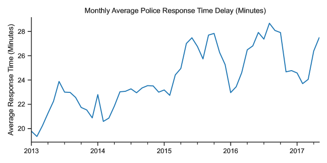
Figure 1: The increasing average police response time in Atlanta by month, from 2013 onwards.

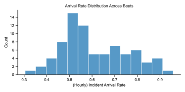
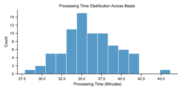
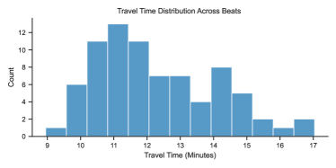
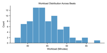
Figure 2: Operations statistics calculated using 911 data from the Atlanta Police Department, from 2013 to 2022, averaged for each of the 80 beats: distribution of hourly incident rate per beat, processing data in minutes, travel time in minutes, workload (the average time an officer need to travel to and process a single incident).

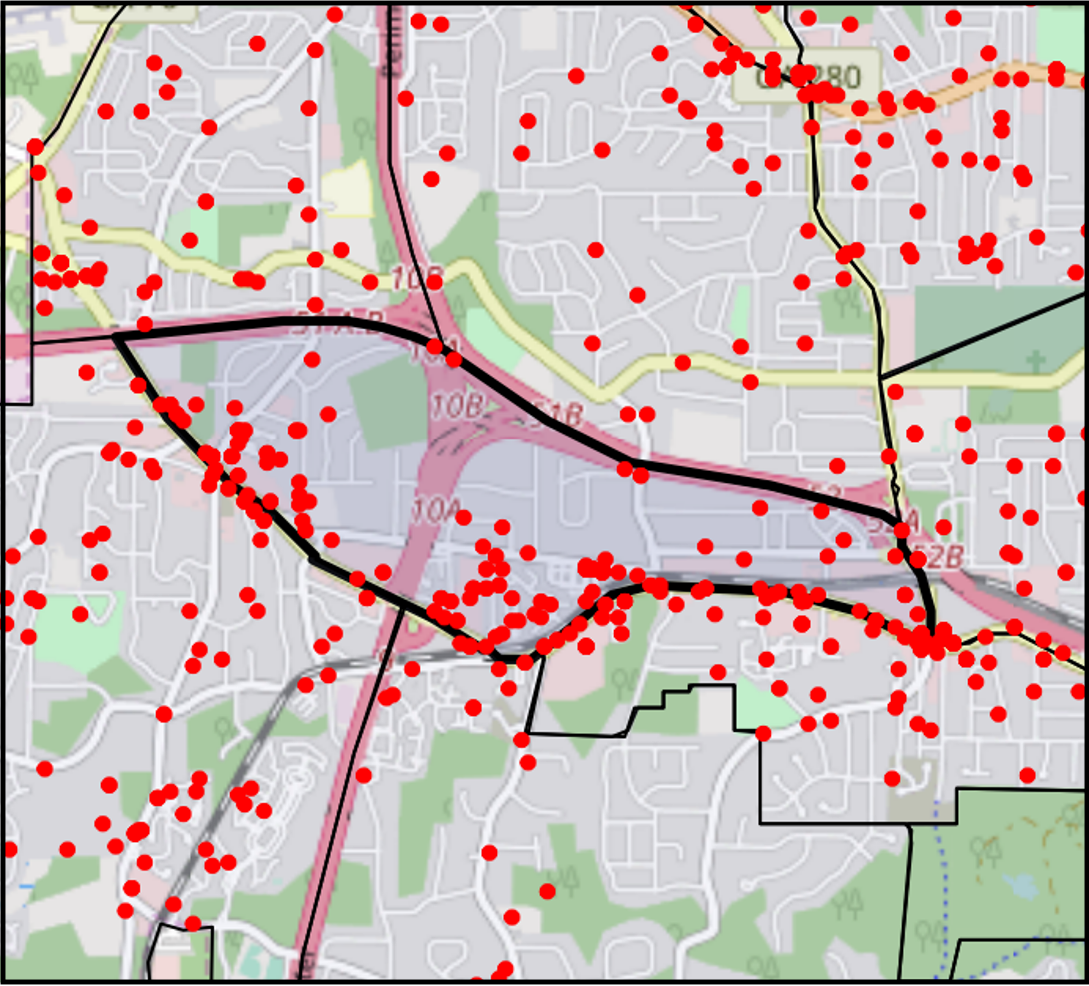
Figure 3: The border effect: Burglary incidents reported by the Atlanta police department in 2017 (represented by red dots) clustered near the border between beats (indicated by black lines).

First, modern police operations, often strained by high workload, necessitate a more flexible queuing model than what is provided by the traditional hypercube queuing model. The hypercube model, while elegant in its simplicity, is limited to representing each server’s status as simply “busy” or “idle” and operates under the assumption of a singular queue for the entire system. However, in today’s context, police operations systems frequently face overwhelming demands, leading to a scenario where all servers are constantly busy, which may not be accurately captured by the hypercube model. Therefore, to effectively understand systems with heavier loads, where there could be multiple queues and each queue might exceed a length of one, our objective is to model the distribution of queue lengths for each server. This approach goes beyond the basic “busy” and “idle” states (represented by binary vectors) used in Larson’s original hypercube queuing models, offering a more detailed and realistic representation of contemporary police operations.

Second, the traditional “one-officer-per-beat” operational mode has become increasingly difficult to implement due to severe staff shortages, which currently pose a significant challenge for many police departments, including those in the Atlanta metro area [7]. For example, as of January 2023, suburban Atlanta’s Gwinnett County (GA) reportedly “employed 690 officers out of an authorized strength of 939, leaving more than a quarter of sworn officer positions vacant” [23]. This leads to busier police operations and challenges in placing at least one officer per beat each day. To address officer shortages in practice, some municipalities have implemented flexible service regions in the middle of their districts, enabling officers to respond to incidents more effectively. This empirical strategy has proven successful. Moreover, by utilizing restricted service regions with some overlap, departments can balance full flexibility and complete isolation, ensuring officers can assist neighboring areas when needed without compromising the efficiency of their primary service areas.

Third, implementing flexible service regions with overlapping beats can help address the so-called “border effect.” For example, in Atlanta, we have observed a notable boundary effect in the distribution of police incidents, with crime rates tending to be higher at the peripheries of police beats (refer to Figure 3 for a burglary case example). Additionally, response times at beat boundaries are often longer due to increased travel distances. Police officers also report that more criminal activity occurs near the borders of two beats, resulting in more 911 calls in these areas. The boundary effect may contribute to increased crime rates near the edges of designated police zones, underscoring the need for a more efficient allocation of law enforcement resources. This observation suggests that the proposed overlapping beat structure may offer the demonstrated theoretical advantages and potential additional benefits in combating the border effect.

Due to the aforementioned motivations, we present a generalized hypercube queuing model in this paper. Our contributions are three-fold: (1) We generalize the classic hypercube queuing model by [13] to study systems at all load levels, including very light, and higher loads all the way up to (strictly smaller than) one. (2) We develop an efficient computational method to estimate the steady-state distribution for systems with a large number of servers; (3) We demonstrate the application of this model to represent the so-called overlapping patrol, where multiple police officers may respond to incidents at the boundaries of patrol regions.

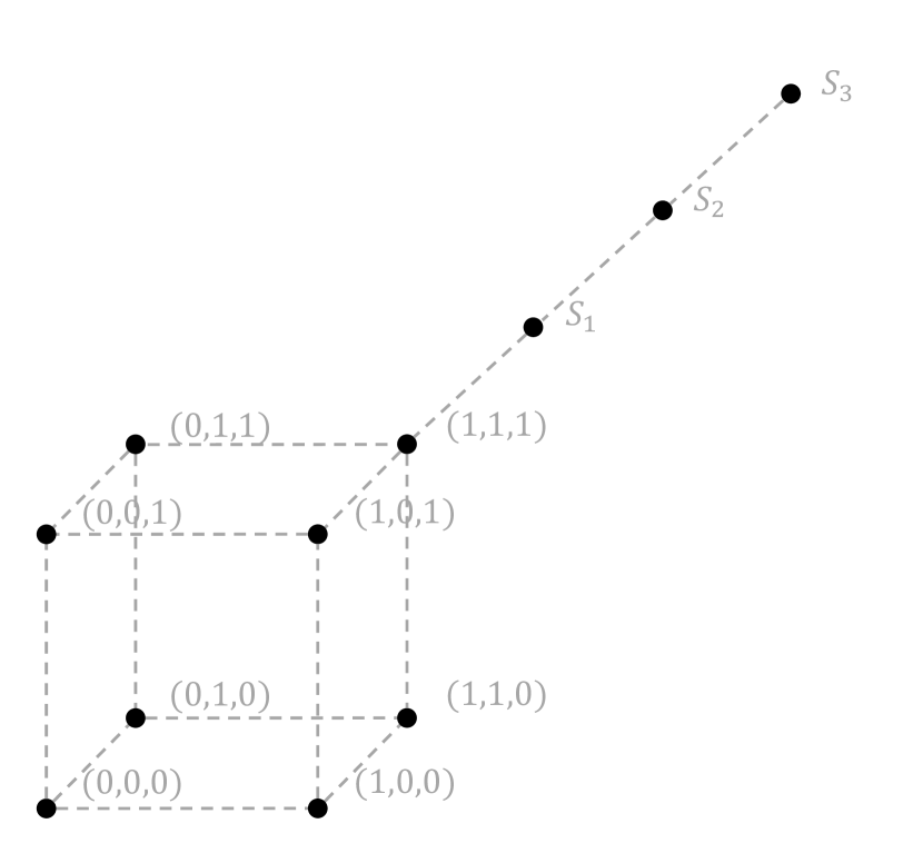
(a) Hypercube

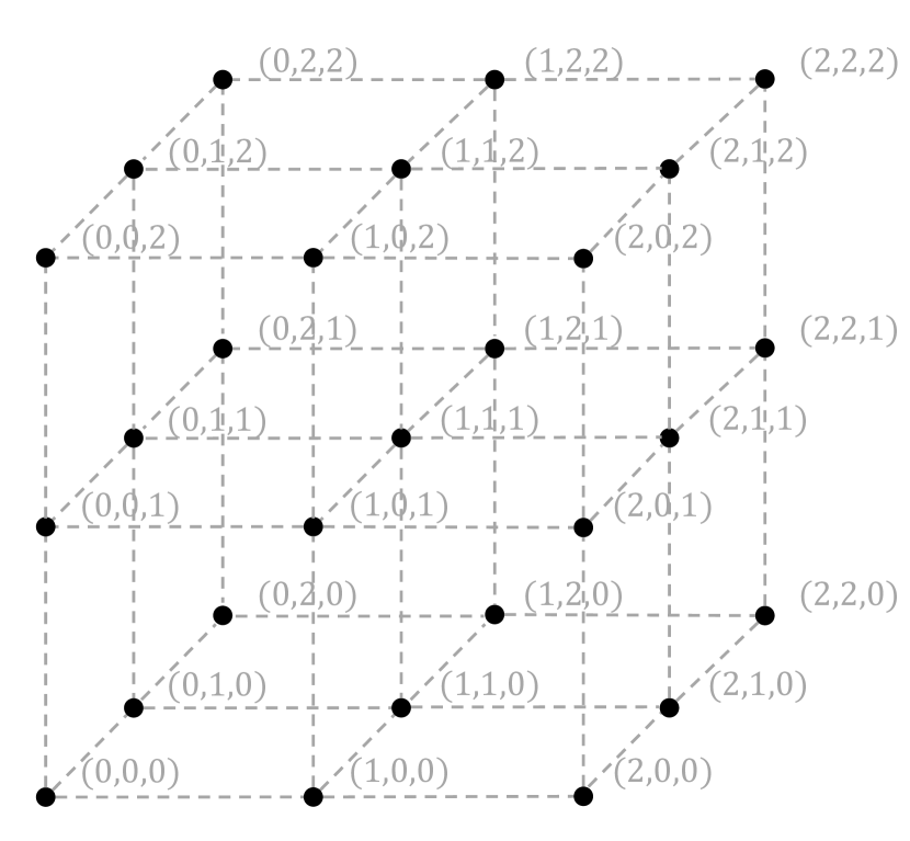
(b) Hyperlattice

Figure 4: Illustration of the differences in state spaces: (a) the traditional Hypercube model and (b) our proposed Hyperlattice model.

To achieve our goal, we consider a Markov model with a potentially large state space represented by integer-valued vectors (in contrast, the hypercube queuing model employs binary-valued state vectors, as shown in Figure 4). The sparse transition matrix allows for transitions between states whose vectors differ by 1 in the $\ell_{1}$ distance (in contrast, the hypercube queuing model considers Hamming distance one transition for binary-valued state vectors). Based on this, we develop an efficient state aggregation technique to relate the generalized hypercube queuing model to the known properties of a general birth-and-death process with state-dependent rates. This reduces the detailed balancing equations to a much smaller linear system of equations, enabling efficient computation for steady-state state distributions, which are key in evaluating general performance metrics as recognized in Larson’s original work [13]. Finally, we validate the effectiveness of the proposed framework by testing it with simulated cases and real-world 911 service call data from Atlanta, Georgia.

This paper is organized as follows: We begin with a review of relevant literature on spatial queuing systems and Markov models with similar structures. In Section 2, we introduce a novel queuing framework for evaluating districting plans with overlapping regions. Section 2.1 discusses the problem setup and key assumptions. Section 2.2 presents a generalized hypercube queuing model – the hyperlattice model – for capturing system dynamics, while Section 2.3 introduces an efficient method for estimating its steady-state distribution. Section 2.4 introduces two key performance measures using the hyperlattice model. Lastly, we demonstrate the effectiveness of our framework through experiments on synthetic systems in Section 3 and conclude in Section 4, discussing potential extensions and generalizations.

1.1 Related works

Spatial queuing systems modeling with overlapping service regions have received limited attention in the literature. However, recent developments in service systems and their growing complexity have spurred an increased interest in this field, particularly in the quest for more efficient dispatch policies. For instance, the concept of overlapping zones is discussed in [4], which only considers completely overlapping service regions. This approach may need to address higher crime rates near boundaries. In contrast, our study focuses on partially overlapping service regions, which are more challenging to analyze but better suited for our purposes.

Richard Larson’s paper [13] and his co-authored book with Asaf Odoni, “Urban Operations Research” [14], introduced the hypercube queuing model, a pioneering work in this field. The hypercube queuing model offers a spatial queuing framework for analyzing and evaluating service systems’ performance. It permits servers to cross over into each other’s territories and provide aid when busy, making it particularly useful for emergency service systems like police and ambulance operations [2, 9, 20, 26, 27, 15]. However, it assumes identical service from all servers sharing a single queue, which may be oversimplified for real-world service systems and unable to capture more complex systems. In our context, servers may have limited authorized movement, resulting in separate queues for each server. This is because other servers cannot travel to specific regions to offer assistance. Consequently, a more flexible model may be necessary to represent such service systems accurately.

Among existing work extending the classic hypercube queuing model for specific applications, a notable contribution is [5], which introduces a variation of the hypercube model. Their extension is designed to represent a dispatch policy in which advanced equipped servers serve solely life-threatening calls (called dedicated servers). Our model, however, differs as it allows servers to operate within the territories of other servers, presenting a distinct problem framework. In addition, they grouped servers with similar characteristics in their state space representation, aiming to lower computational demands. In our method, each server is still represented individually in the state space, managing to do so without significant computational expense. We also assume each server has its own queue, diverging from most Hypercube model variations that use a single queue for all servers.

Recently, [21] introduced a flexible queue architecture for a multi-server model, comprising $n$ flexible servers and $n$ queues connected through a bipartite graph, with each server having its own associated queue. The paper mainly focuses on the model’s theoretical aspects and addresses the essential benefits of flexibility and resource pooling in such queuing networks. They specifically concentrate on the scaling regime where the system size $n$ tends to be infinite while overall traffic intensity remains constant. However, their model cannot be directly extended to our scenario, as it does not consider the geographical relationship among servers.

Other related works analyze service systems using similar modeling techniques [8]. For example, [3] proposes a new approximate hypercube spatial queuing model similar to the hyperlattice model, allowing multiple servers to be located at the same station and multiple servers to be dispatched to a single call. The state space of their model can be represented by a vector of non-negative integer, where the $i$-th integer indicates the number of calls in the system that are being served by the $i$-th server. Rather than reducing to a birth-death process, they use the M[G]/M/s/s queuing model to derive approximate formulas for the hypercube spatial queuing outputs. In [11], the paper describes a model developed to represent patrol car operations accurately. It is a multi-priority queuing model explicitly reflecting multiple car dispatches. Instead of focusing on overlapping patrol, this paper aims to provide a better basis for efficient patrol car allocation and enables police officials to evaluate policies, such as one-officer patrol cars, that affect the number of cars dispatched to various incident types. In [22], the authors examine similar systems where each server can handle a specific subset of “job types”, which can be seen as calls received in different regions. The proposed solution retains the identity and position of busy servers but does not indicate the particular job type being handled. Specifically, it only tracks the number of jobs between busy servers without specifying the sequence of job types. However, like the Hypercube queuing model, this model has a single queue where incoming jobs without feasibly available servers wait and are processed in a First-Come-First-Served order. As a result, this model is not directly applicable to represent service systems of interest with multiple queues in overlapping service regions. A recent paper [24] studies a distinct server routing-scheduling problem in a distributed queuing system, unlike the problem we are examining in this paper. This system consists of multiple queues at different locations. In such a system, servers are allocated across multiple queues and move among these queues to meet demands that are both random and fluctuate over time. Another paper [1] proposes a similar approach, modeling the system as a Markov process but delaying the discovery of a job’s type until a server needs to know the type. In comparison, our system does not differentiate calls (or job types) in any server. Another key difference is that this paper aims to derive exact asymptotics of stationary distributions from analyzing production contexts where the fluid limit of excursions to the increasingly rare event is nonlinear.

2 Proposed framework

This section develops a framework for assessing districting plans with overlapping patrol units for service systems. To gain insight into the strategy of overlapping patrol, we consider a moving-server queuing system with multiple servers. Typically, each server (e.g., a patrol service unit) is assigned to one particular service region, where the server has primary responsibility. When a server is not busy serving any active calls, it traverses its home region to perform preventive patrol. A key feature of our model is that multiple servers are allowed to be jointly responsible for a third overlapping service region besides their respective home regions, as illustrated in Figure 5. For the reader’s convenience, Table 1 contains summary definitions of notations frequently used in the paper.

Table 1: Summary of key notations

Section	Notation	Description
2.1	$I$	Total number of servers.
	$\mathcal{I}=\{i=1,\dots,I\}$	Set of indices of servers as well as their primary service regions.
	$\mathcal{E}=\{e\in\mathcal{I}\}$	Set of overlapping service regions.
	$\lambda_{i}$	Arrival rate of primary service region $i$.
	$\lambda_{e}$	Arrival rate of overlapping service region $e$.
	$\lambda$	Arrival rate within the entire region of interest.
	$\mu_{i}$	Service rate of server $i$.
	$\mu$	Total service rate of all servers.
2.2	$n_{i}\in\mathbb{Z}_{*}$	Status of server $i$. Server $i$ is idle if $n_{i}=0$ and busy if $n_{i}>0$.
	$\eta_{e,u}(i)\in[0,1]$	Probability of choosing server $i$ in overlapping region $e$ at state $u$.
	$B=(n_{i})_{i\in\mathcal{I}}$	A state (node) in the hyperlattice.
	$\mathcal{U}=\{u=1,2,\dots\}$	Set of state indices ordered by the tour algorithm.
	$Q=(q_{uv})_{u,v\in\mathcal{U}}$	Transition rate matrix for the hyperlattice queue.
2.3	$N_{k}$	A state in the aggregate (birth-death) model
	$\bar{\lambda}_{k}$	Birth rate of aggregated state $N_{k}$.
	$\bar{\mu}_{k}$	Death rate of aggregated state $N_{k}$.
	$U_{K}$	Number of states where the total number of calls in the system is less than $K$.
	$\mathcal{U}_{K}=\{u=1,\dots,U_{K}\}$	Set of states for the truncated hyperlattice queue.
	$Q_{K}=(q_{uv})_{u,v\in\mathcal{U}_{K}}$	Transition rate matrix for the truncated hyperlattice queue.
2.4	$\rho_{i}$	Fraction of time that server $i$ is busy serving calls.
	$\rho_{i,e}/\rho_{i,i}$	Fraction of dispatches that send server $i$ to each sub-region $e$ (or $i$).

2.1 Problem setup and key assumptions

In this section, we describe our problem setup and several key assumptions. Consider a service system patrolled by multiple servers, where each server is allocated to a specific area. Unlike conventional service systems with separate service territories, our approach permits servers to have overlapping service areas. The entire service system can be represented by an undirected hypergraph [6] denoted by $(\mathcal{I},\mathcal{E})$. In this hypergraph, $\mathcal{I}=\{i=1,\dots,I\}$ denotes the set of vertices, each representing an individual server, with $I$ being the total number of servers in the system. The set $\mathcal{E}$ represents hyperedges, each of which corresponds to a group of servers denoted as $e\in\mathcal{E}\subseteq\mathcal{I}$, jointly overseeing an overlapping area. The cardinality of $\mathcal{E}$ is denoted by $E$. Figure 6 presents the hypergraph of a three-server system as an example.

The service system encompasses a geographical space denoted by $\mathcal{S}\subset\mathbb{R}^{2}$. We denote the part of the space that server $i$ patrols as $\mathcal{S}_{i}\subseteq\mathcal{S}$. We require that the service territories of all servers cover the entire space of the system, i.e., $\bigcup_{i\in\mathcal{I}}\mathcal{S}_{i}=\mathcal{S}$. Regions jointly patrolled by a set of servers $e\in\mathcal{E}$, are termed as overlapping service regions, and are denoted as $\mathcal{O}_{e}$. Conversely, regions exclusively patrolled by server $i$ are termed primary service regions, and are defined as $\mathcal{P}_{i}=\mathcal{S}_{i}\backslash\bigcup_{\{e:i\in e\}}\mathcal{O}_{e}$. Note that it is important to guarantee $e\not\subseteq e^{\prime}$ for every $e,e^{\prime}\in\mathcal{E}$ and $e\neq e^{\prime}$. This ensures all primary and overlapping service regions are mutually exclusive and can be distinctly identified either by $i\in\mathcal{I}$ or by $e\in\mathcal{E}$. Both primary and overlapping service regions can be arbitrarily small to avoid quantization errors, and they can have any geometric shape.

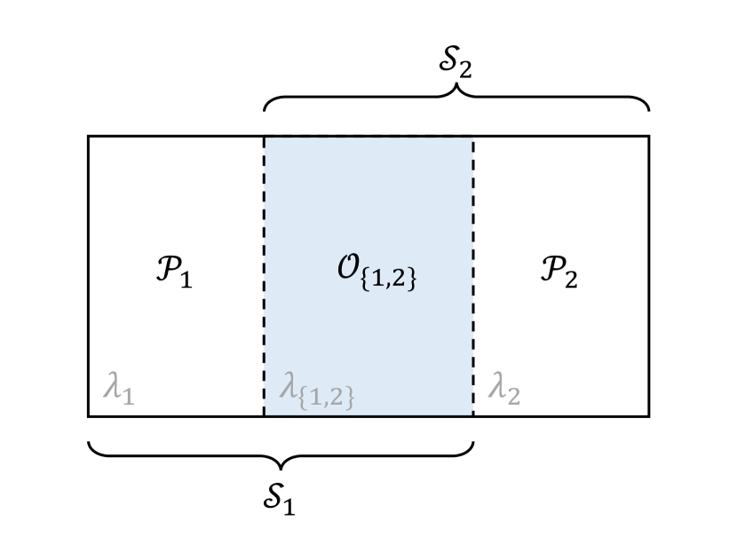
(a) Two-server system

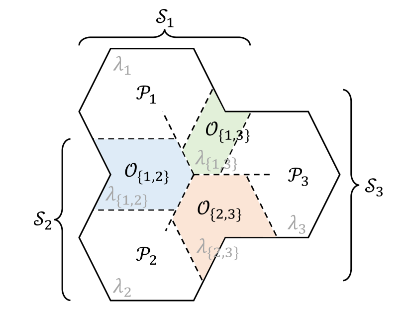
(b) Three-server system

Figure 5: Examples of three service systems with overlapping patrol. The white area $\mathcal{P}_{i}$ indicates primary service region $i$ that can only be served by server $i$ and the shaded area $\mathcal{O}_{e}$ indicates overlapping service region $e=\{i,j\}$ that can be jointly served by servers $i$ and $j$.

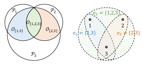
Figure 6: The hypergraph of a three-server system, where the black dots represent vertices and the shaded areas represent hyperedges.

Assume service calls arrive in the system according to a general stationary arrival process. The arrivals of calls in primary service region $i$ and overlapping service region $e$ follow time-homogeneous Poisson processes with rate $\lambda_{i}$ and $\lambda_{e}$, respectively. Let $\lambda=\sum_{i\in\mathcal{I}}\lambda_{i}+\sum_{e\in\mathcal{E}}\lambda_{e}$ be the aggregate call arrival rate in the entire region.

The service process is described as follows. The server starts to process the call as soon as it arrives at the location where the call is reported. The service time of each server is independent of the location of the customer and the history of the system; The service time of server $i$ for any call for service has a negative exponential distribution with mean $1/\mu_{i}$. Let $\mu=\sum_{i\in\mathcal{I}}\mu_{i}$ denote the aggregate service rate in the entire region. After finishing the service, the server stays at the same location until receiving a new call from the dispatch center. For ergodicity, it is necessary that $\lambda<\mu$ should hold.

We assume each server has its own queue, with the dispatch policy being state-dependent. For the sake of simplicity in presenting our findings, we start our discussion with a traditional setup that many service systems typically use. Then we will show that our assumptions can be applied more broadly across various service systems. In the traditional context, we adopt the following dispatch policy: If a call arrives in the service region of a server and finds the server available (randomly choose a server if there is more than one), then it goes into service upon the server’s arrival. When there is no server available, the dispatch policy can be discussed in the following three situations:

1. If the call arrives in the primary service region of a server, it joins the end of the queue of the server.

2. If a call is received in the overlapping service region, the call will be randomly assigned to one of the available servers that are in charge of this region.

3. If a call is received in the overlapping service region and there is no available server, the call will be randomly assigned to one of the responsible servers, and wait in its corresponding queue until the server becomes available.

An example of the dispatch policy for a two-server system with one overlapping service region is presented in Figure 7.

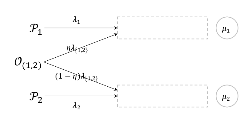
(a) Both idle

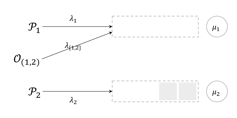
(b) One busy

(c) Both busy

Figure 7: Queue networks with two servers and two queues when (a) both servers are idle, (b) one of the servers is busy, and (c) both servers are busy, where $\eta$ is the probability of assigning the call to server $i$.

2.2 Hyperlattice queuing model for overlapping patrol

We propose a generalized hypercube queuing model, called the hyperlattice model, to capture the operational dynamics of systems with overlapping service regions. The system state depends on the status of all the servers in this system, and the number of calls in each queue to be processed.

2.2.1 State representation

These states can be represented by a hyperlattice in dimension $I$. Each node of the hyperlattice corresponds to a state $B=(n_{i})_{i\in\mathcal{I}}$ represented by a tuple of numbers, where non-negative integer $n_{i}\in\mathbb{Z}_{*}$ indicates the status of server $i$. Server $i$ is idle if $n_{i}=0$ and busy if $n_{i}>0$. The value of $n_{i}-1$ represents the number of calls waiting in the queue of server $i$ when the server is busy. Figure 8 (a) gives an example of the state space of a hyperlattice queuing model for a system with two servers. It is worth noting that the state space in a hyperlattice queuing model can be divided into two parts, with one part consisting of states that possess at least one available server (referred to as non-saturated states) and the other part comprising states in which all servers are busy (referred to as saturated states), as shown in Figure 9.

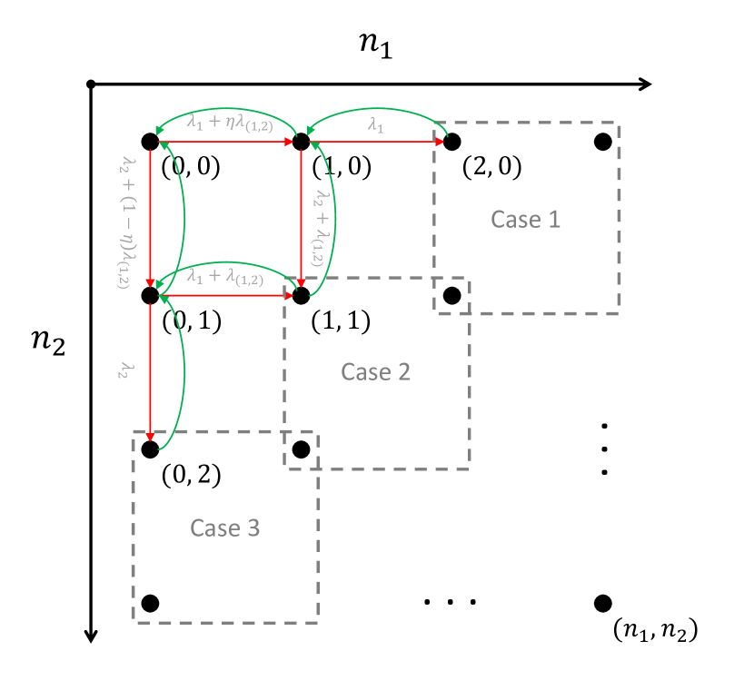
(a) State space

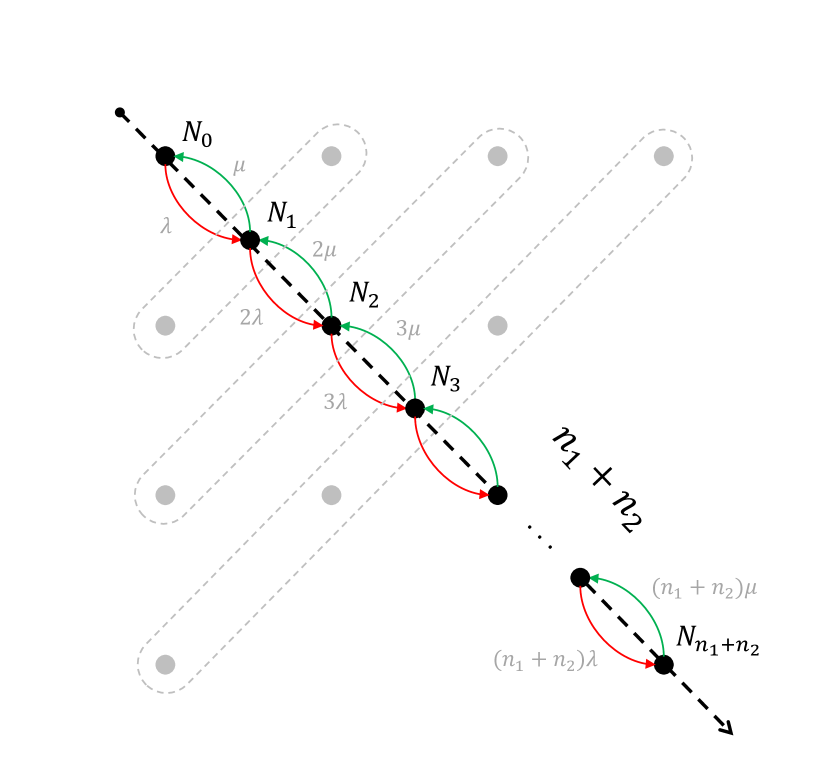
(b) Aggregated state space

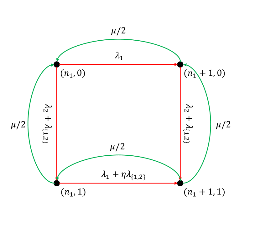
(c) Case 1: for $n_{1}\geq 1$ and $n_{2}<1$

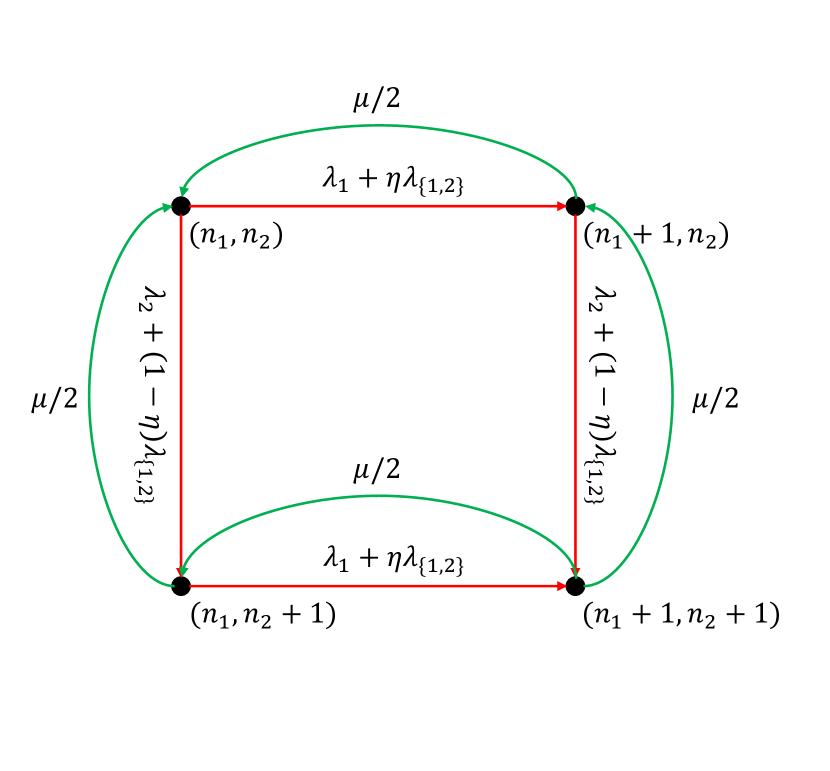
(d) Case 2: for $n_{1},n_{2}\geq 1$

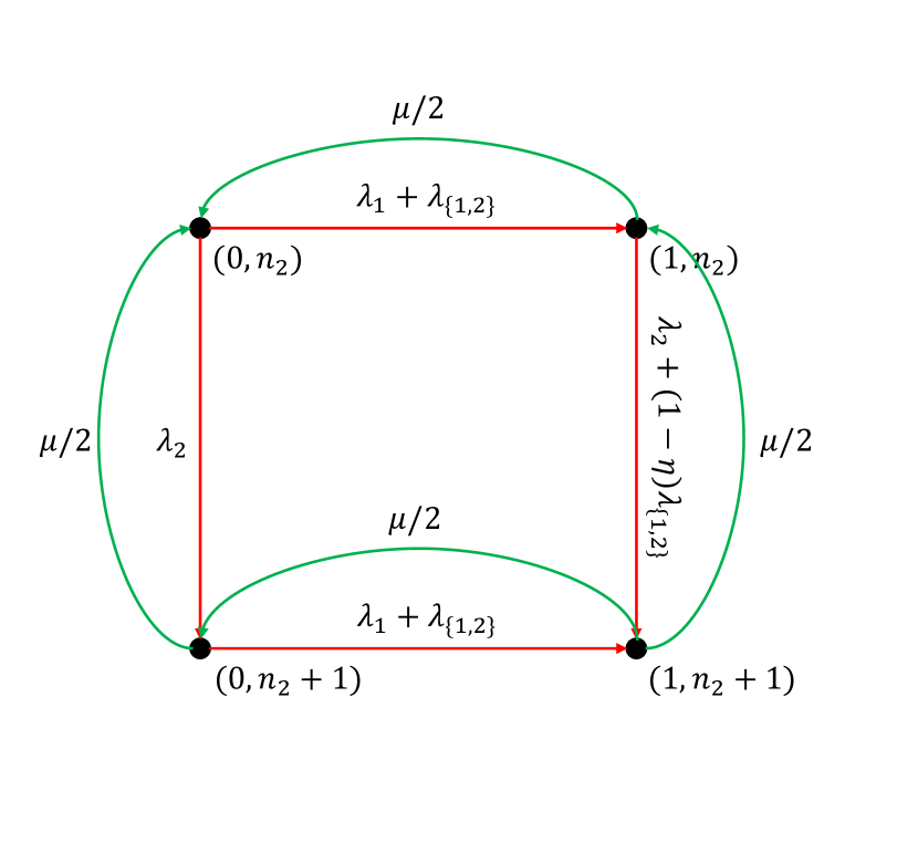
(e) Case 3: for $n_{1}<1$ and $n_{2}\geq 1$

Figure 8: The state space in a hyperlattice queuing model for a system with two servers of equal service rate $\mu/2$. The state space is shown in (a) as an overview, with each state denoted by the pair $(n_{1},n_{2})$. Green arrows indicate downward transitions and red arrows indicate upward transitions. (b) presents the birth-death model by aggregating states that share the same value of $n_{1}+n_{2}$. In (c), (d), and (e), the details of the state space are depicted in three distinct scenarios.

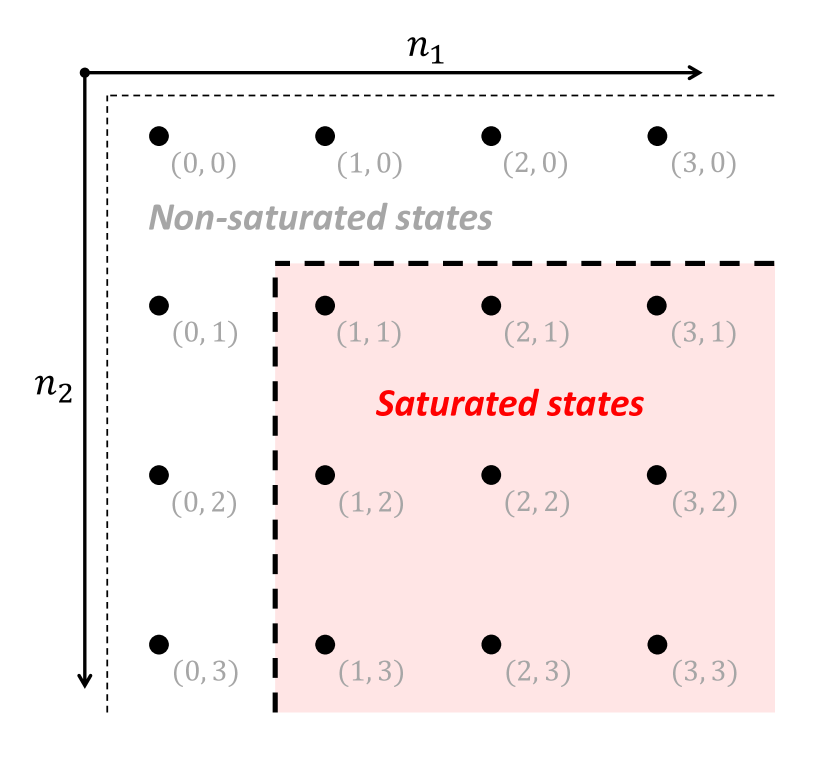
(a) Two servers

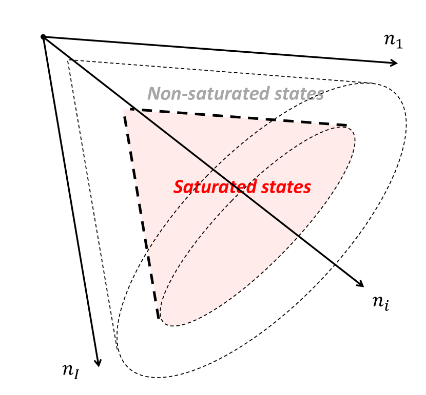
(b) $I$ servers

Figure 9: An illustration of two types of states in hyperlattice queuing models with different numbers of servers. The area colored red signifies the saturated states that have no idle servers, whereas the empty area represents the non-saturated states that have at least one server that is unoccupied.

2.2.2 Touring algorithm

To create the transition rate matrix, the states must be arranged in order. However, since the standard vector space lacks an inherent order, we employ a touring algorithm to traverse the entire hyperlattice. This algorithm generates a sequence of $I$-digit non-negative integers $B_{0},B_{1},\dots$, which contains an infinite number of members and fully describes the order of the states.

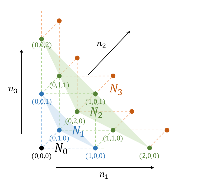
(a) State space

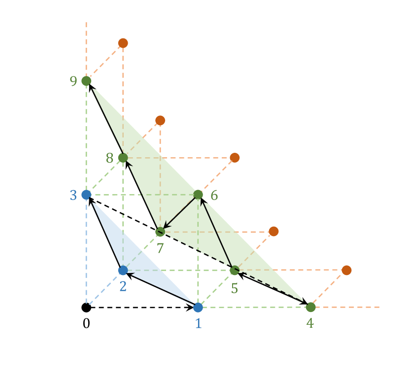
(b) Tour of all states with $k\leq 3$

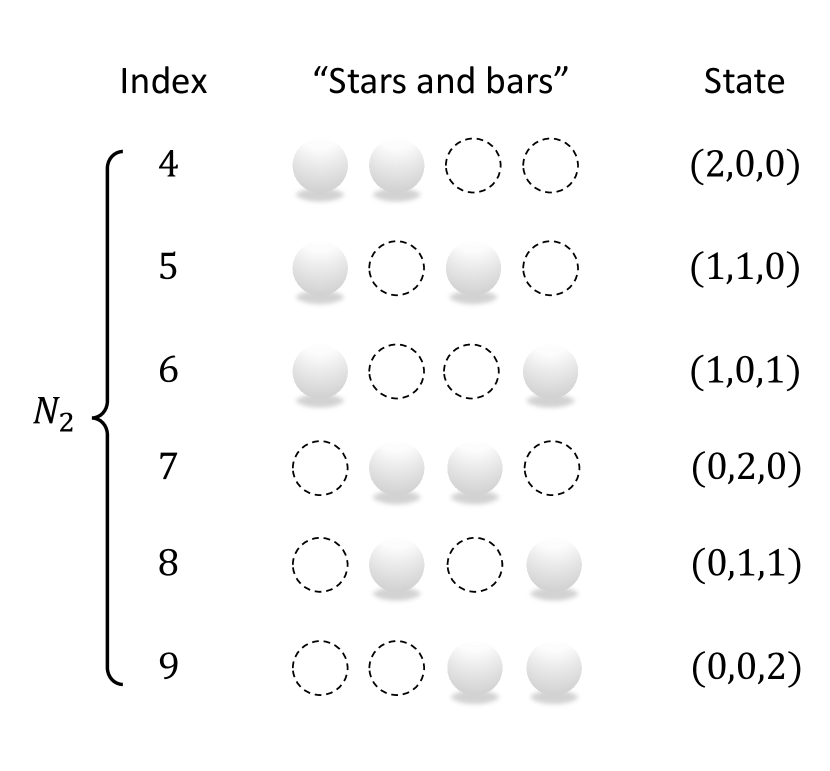
(c) Tour within $N_{2}$

Figure 10: A hyperlattice queuing model for a system with three service regions. (a) shows part of the state space of the hyperlattice for $k=1,2,3$; (b) presents the tour of all the states with $k\leq 3$, where solid arrows represent the tour within an aggregated state and dashed arrows represent the tour across aggregated states; (c) shows the sequence of all the states in the aggregated state $N_{2}$, where the number of balls separated by dashed circles represents the status of server $i$ ($n_{i}$).

Input: Number of servers $I$; Output: The sequence of ordered states $\mathcal{B}$;

Initialization: $\mathcal{B}\leftarrow\emptyset$;

for $k=0,1,\dots$ do

       $\mathcal{B}_{k}\leftarrow\{(n_{i})\in\mathbb{Z}_{*}^{I}\mid\sum_{i\in\mathcal{I}}n_{i}=k\}$; // $|\mathcal{B}_{k}|=\binom{k+I-1}{I-1}$

       Sort $\mathcal{B}_{k}$ using an arbitrary order;

       $\mathcal{B}\leftarrow(\mathcal{B},\mathcal{B}_{k})$;

      

end for

Algorithm 1 Tour algorithm for a hyperlattice

We simplify the tour problem by decomposing it into $K$ sub-problems. Each sub-problem $k\leq K$ first identifies the states in which exactly $k$ calls are staying in the system (either waiting in the queue or being served), and then proceeds to solve the enumerative combinatorics problem by searching for $\binom{k+I-1}{I-1}$ possible combinations in a pre-determined sequence. It is important to note that the sequence generated by each sub-problem is just one of numerous possible tours of the cutting plane in the hyperlattice. Figure 10 presents a hyperlattice with $I=3$, along with its corresponding tour of all the states. The combinatorics can be translated into the “stars and bars” [10], i.e., finding all possible positions of $I-1$ dashed circles that separate $k$ balls into $I$ groups, as illustrated in Figure 10 (c). The number of balls being separated in group $i$ can be regarded as $n_{i}$. Algorithm 1 summarizes the tour algorithm that generates the sequence $B_{0},B_{1},\dots$. For convenience, we index the states based on the order produced by the tour algorithm. The state index is represented by $u\in\mathcal{U}=\{0,1,2,\dots\}$.

2.2.3 Transition rate matrix

Now we define the transition rate matrix for the hyperlattice queue $Q=(q_{uv})_{u,v\in\mathcal{U}}$, where $q_{uv}$ ($u\neq v$) denotes the transition rate departing from state $B_{u}$ to state $B_{v}$. Let $u$ represent the index of state $(n_{1},n_{2},\dots,n_{i},\dots,n_{I})$ and let $d_{uv}=\left\lVert B_{u}-B_{v}\right\rVert_{1}$ be the $\ell_{1}$ distance (or Manhattan distance) between two vertices $B_{u}$ and $B_{v}$ on the hyperlattice. We define $u^{i+}$ as the index of state $(n_{1},n_{2},\dots,n_{i}+1,\dots,n_{I})$; note that thus we have $d_{uu^{i+}}=1$ and $B_{u^{i+}}\succ B_{u}$ ($B_{u}$ is elementwise greater than $B_{v}$). Diagonal entries $q_{uu}$ are defined such that $q_{uu}=-\sum_{v:v\neq u}q_{uv}$ and therefore the rows of the matrix sum to zero. There are two classes of transitions on the hyperlattice: upward transitions that change a server’s status from idle to busy or add a new call to its queue; and downward transitions that do the reverse. The downward transition rate from state $B_{u^{i+}}$ to its adjacent state $B_{u}$ is always $q_{u^{i+}u}=\mu_{i}$. The upward transition rate, however, will depend on how regions overlap with each other and the dispatch rule when a call is received, which can be formally defined by the following proposition.

Proposition 1 (Upward transition rate).

For an arbitrary state index $u$, the upward transition rate from $B_{u}$ to $B_{u^{i+}}$ is:

$$q_{uu^{i+}}=\lambda_{i}+\sum_{e\in\mathcal{E}}\eta_{e,u}(i)\lambda_{e},$$ (1)

where $\eta_{e,u}(\cdot)$ is a probability mass function that gives the probability of the new call in the overlapping service region $\mathcal{O}_{e}$ being received by server $i\in e$ at state $B_{u}$. The probability mass function $\eta_{e,u}$ has the following properties:

$$\eta_{e,u}(i) =0, ~{}\forall i\notin e,e\in\mathcal{E},$$ (2)

$$\sum_{i\in\mathcal{I}}\eta_{e,u}(i) =1, ~{}\forall e\in\mathcal{E}.$$ (3)

The following argument justifies the proposition. The first term of (1) suggests that, for an arbitrary server $i$, it must respond to a call received in its primary service region $i$. The second term of (1) means that the server $i$ needs to respond to a call received in the overlapping service region $e$ according to the dispatch policy $\eta_{e,u}$. It is important to emphasize that the dispatch policy $\eta_{e,u}$ is state-dependent and can be defined based on the user’s needs, offering a general framework that is apt for elucidating both random and deterministic dispatch strategies. For example, the one outlined in Section 2.1 represents a specific case of the dispatch policy, in which the assignment of server $i$ to the call received in overlapping service region $e$ can be discussed in two scenarios: (a) When all servers $i\in e$ are busy ($u:n_{i}>0,\forall~{}n_{i}\in B_{u}$), this call will join the queue of server $i$ based on the probability $\eta_{e,u}(i)$. (b) Conversely, when there is at least one server idle ($u:n_{i}=0,n_{i}\in B_{u}$), the server $i$ will be assigned to this call based on the probability $\eta_{e,u}(i)$. In Appendix, we also demonstrate how this proposition can be distilled to represent a rudimentary system where, at most, only two servers are permitted to patrol one overlapping service region.

2.2.4 Balance equations

To obtain the steady-state probabilities of the system, we can solve the balance equations given the transition rate matrix $Q$. Let $\mathbb{P}\{B\}$ denote the probability that the system is occupying state $B$ under steady-state conditions. The balance equations can be written as:

$$\left(\sum_{v:{B_{v}\succ B_{u}\atop d_{uv}=1}}q_{uv}+\sum_{v:{B_{u}\succ B_{v}\atop d_{uv}=1}}q_{uv}\right)\mathbb{P}\{B_{u}\}=\sum_{v:{B_{u}\succ B_{v}\atop d_{vu}=1}}q_{vu}\mathbb{P}\{B_{v}\}+\sum_{v:{B_{v}\succ B_{u}\atop d_{vu}=1}}q_{vu}\mathbb{P}\{B_{v}\},\quad u\in\mathcal{U}.$$ (4)

We also require that the probabilities sum to one, namely,

$$\sum_{u\in\mathcal{U}}\mathbb{P}\{B_{u}\}=1.$$

However, the above balance equations cannot be solved computationally as the number of states on the hyperlattice is infinite and grows exponentially with the number of servers even when queue capacity is limited. To overcome this difficulty, we introduce an efficient estimation strategy in the next section.

2.3 Efficient steady-state distribution estimation

Now we introduce an efficient computational method to estimate the steady-state distribution that particularly leverages the symmetrical structure of the state space and the sparsity of its transition rate matrix.

2.3.1 Aggregated states and queue length distribution

We first exploit the fact that the hyperlattice queuing model in the aggregate is simply a birth-death model whose states can be represented by $\{N_{k}\}_{k=0,1,\dots,\infty}$ and $k$ can be interpreted as the number of calls currently in the system. This equivalence is obtained by collecting together all states having an equal value of $k=\left\lVert B\right\rVert_{1}$ as shown in Figure 8 (b). Their summed steady-state probability is equal to the comparable probability of state occurring in the birth-death model, i.e.,

$$\sum_{B:\left\lVert B\right\rVert_{1}=k}\mathbb{P}\{B\}=\mathbb{P}\{N_{k}\}.$$ (5)

The birth and death rates of the aggregated model can be defined by the following proposition:

Proposition 2.

The birth rate and death rate of the aggregated state $N_{k}$, represented by $\bar{\lambda}_{k}$ and $\bar{\mu}_{k}$ respectively, can be expressed as follows:

$$\bar{\lambda}_{k}= ~{}\binom{k+I-1}{I-1}\lambda,\quad k=0,1,\dots,$$ (6)

$$\bar{\mu}_{k}= ~{}\binom{k+I-2}{I-1}\mu,\quad k=1,2,\dots.$$

Proof.

To begin with, we define $\bar{\lambda}\left(B_{u}\right):=\sum_{i\in\mathcal{I}}q_{uu^{i+}}$ as the total sum of upward transition rates originating from an arbitrary state $B_{u}$. Given the upward transition rates that leave state $B_{u}$ defined in (1), we have

$$\bar{\lambda}\left(B_{u}\right) =\sum_{i\in\mathcal{I}}q_{uu^{i+}}=\sum_{i\in\mathcal{I}}\left[\lambda_{i}+\sum_{e\in\mathcal{E}}\eta_{e,u}(i)\lambda_{e}\right]=\sum_{i\in\mathcal{I}}\lambda_{i}+\sum_{e\in\mathcal{E}}\lambda_{e}\left[\sum_{i\in\mathcal{I}}\eta_{e,u}(i)\right]$$

$$\stackrel{{\scriptstyle(i)}}{{=}}\sum_{i\in\mathcal{I}}\lambda_{i}+\sum_{e\in\mathcal{E}}\lambda_{e}=\lambda$$

where the equation $(i)$ holds due to (3). Hence, the sum of all upward transition rates leaving any given state is constantly $\lambda$.

Now the birth rate of the aggregated state $N_{k},~{}k\geq 0$ can be obtained by multiplying $\bar{\lambda}(B_{u})$ by the number of states that are part of $N_{k}$, which is equivalent to $\binom{k+I-1}{I-1}$. It is also evident that the total of all downward transition rates leading to an arbitrary state is $\sum_{i\in\mathcal{I}}\mu_{i}$, which is equal to $\mu$. Consequently, we can obtain the death rate of $N_{k},~{}k\geq 1$ similarly by multiplying the total service rate $\mu$ by the number of states included in $N_{k}$. ∎

Remark 1.

The birth and death rates in the aggregated model are solely determined by the total arrival rate $\lambda$ and service rate $\mu$, and both rates increase exponentially with respect to $k$. If we let $n=k+I-1$ and $m=I-1$, we can use Stirling’s Formula [19] to obtain the asymptotic expression for $\binom{n}{m}$:

$$\frac{\sqrt{2\pi n}(n/e)^{n}}{m!\sqrt{2\pi(n-m)}((n-m)/e)^{n-m}}=(1-m/n)^{m-1/2}\frac{e^{-m}}{m!(1-m/n)^{n}}n^{m}.$$

It is worth noting that the first term on the right-hand side of the equation approaches 1 as $n\rightarrow\infty$. Additionally, the denominator of the middle term on the right-hand side approaches $m!e^{-m}$, which means that the middle term also approaches $1/m!$. Therefore, we can approximate the rate of growth as follows when $k\rightarrow\infty$:

$$\binom{k+I-1}{I-1}\approx\frac{(k+I-1)^{I-1}}{(I-1)!}.$$

Figure 11 shows the effect of $I$ and $k$ on the birth and death rates of hyperlattice queuing models.

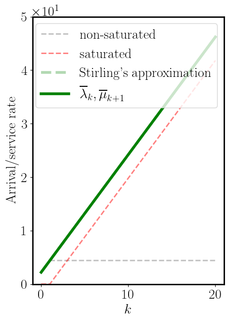
(a) Two servers

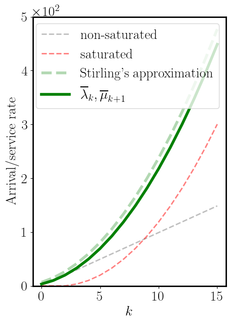
(b) Three servers

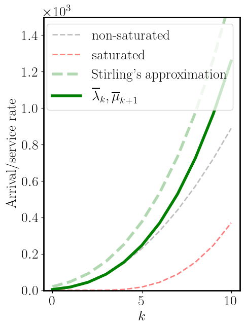
(c) Four servers

Figure 11: The effect of the number of servers on the birth and death rates of hyperlattice queuing models with $\lambda=\mu=I$. The upward transition rates, both from non-saturated states (represented by gray dashed line) in $N_{k}$ and saturated states (represented by red dashed line) in $N_{k}$, to states in $N_{k+1}$ are shown collectively.

Now, rather than attempting to calculate the stationary distribution across an infinite number of states in the original state space, the problem can be simplified by focusing only on a finite subset of states. These states are selectively considered if their $k$ values are less than a user-defined hyper-parameter $K$, or $\left\lVert B\right\rVert_{1}\leq K$, and the sum of their steady-state probabilities remains constant. The choice of $K$ will discussed below and verified by an example in Table 2. Proposition 3 provides a closed-form formula for the steady-state probability of the aggregate state $N_{k}$ when $k\leq K$.

Proposition 3 (Distribution of aggregated queue length).

The probabilities of aggregated states can be written in closed-form using (6) as in a birth-death model

$$\mathbb{P}\{N_{k}\}=\left(\prod_{l=1}^{k}\frac{\bar{\lambda}_{l-1}}{\bar{\mu}_{l}}\right)\left(\sum_{k^{\prime}=1}^{\infty}\frac{\prod_{l=0}^{k^{\prime}-1}\bar{\lambda}_{l}}{\prod_{l=1}^{k^{\prime}}\bar{\mu}_{l}}\right)^{-1}.$$ (7)

Proof.

The proof is as follows. In a steady state for a continuous-time Markov chain, the rate at which individuals transition into a particular state must be equal to the rate at which individuals transition out of that state. Recall that the birth and death rate of aggregated state $N_{k}$ are denoted by $\bar{\lambda}_{k}$ and $\bar{\mu}_{k}$, respectively, and $\mathbb{P}\{N_{k}\}$ is the probability of being in state $N_{k}$, then we have the set of equations:

$$\bar{\lambda}_{0}\mathbb{P}\{N_{0}\}= ~{}\bar{\mu}_{1}\mathbb{P}\{N_{1}\},$$

$$(\bar{\lambda}_{k}+\bar{\mu}_{k})\mathbb{P}\{N_{k}\}= ~{}\bar{\lambda}_{k-1}\mathbb{P}\{N_{k-1}\}+\bar{\mu}_{k+1}\mathbb{P}\{N_{k+1}\},\quad k>1.$$

The first equation gives us $\mathbb{P}\{N_{1}\}=(\bar{\lambda}_{0}/\bar{\mu}_{1})\mathbb{P}\{N_{0}\}$ and the second equation suggests that:

$$\mathbb{P}\{N_{k+1}\}=\frac{(\bar{\lambda}_{k}+\bar{\mu}_{k})\mathbb{P}\{N_{k}\}-\bar{\lambda}_{k-1}\mathbb{P}\{N_{k-1}\}}{\bar{\mu}_{k+1}}=\frac{(\bar{\lambda}_{k}+\bar{\mu}_{k})\mathbb{P}\{N_{k}\}-\bar{\mu}_{k}\mathbb{P}\{N_{k}\}}{\bar{\mu}_{k+1}}=\frac{\bar{\lambda}_{k}}{\bar{\mu}_{k+1}}\mathbb{P}\{N_{k}\}.$$

Therefore, we have

$$\mathbb{P}\{N_{k}\}=\frac{\prod_{l=0}^{k-1}\bar{\lambda}_{l}}{\prod_{l=1}^{k}\bar{\mu}_{l}}\mathbb{P}\{N_{0}\}.$$ (8)

Assuming that the birth and death rates are such that we actually have well-defined steady-state probabilities, $\sum_{k=0}^{\infty}\mathbb{P}\{N_{k}\}=1$, and so

$$\sum_{k=1}^{\infty}\frac{\prod_{l=0}^{k-1}\bar{\lambda}_{l}}{\prod_{l=1}^{k}\bar{\mu}_{l}}\mathbb{P}\{N_{0}\}=1,$$

which implies the desired result. ∎

It is worth noting that the probabilities of the “tail” of the hyperlattice (states with large $k$ value) are usually low and can be negligible since their chance of happening decreases with the length of the queue. As a result, it is empirically benign to ignore the tail of the hyperlattice and focus on the states where the total number of calls in the system is less than $K$. We represent this set of states by $\mathcal{U}_{K}=\{0,\dots,U_{K}\}$, where $U_{K}$ denotes the size of the set. In the subsequent discussion, Lemma 1 presents the equation for $U_{K}$ in relation to $K$ and $I$. This demonstrates that the size of the set can expand exponentially relative to the number of servers $I$, and it can become quite substantial even for moderate values of $K$, particularly in systems with multiple servers.

Lemma 1.

The size of the set $\mathcal{U}_{K}$ is $U_{K}=\binom{K+I}{I}$.

Proof.

The size of the set $\mathcal{U}_{K}$ is equal to the summation $U_{K}=\sum_{k=0}^{K}\binom{k+I-1}{I-1}$, which can be simplified using the Hockey Stick identity [12]:

$$\sum_{k=n}^{m}\binom{k}{n}=\binom{m+1}{n+1}.$$

Applying the identity with $m=I-1$ and $n=K+I-1$, we get:

$$\sum_{k=0}^{K}\binom{k+I-1}{I-1}=\sum_{k=I-1}^{K+I-1}\binom{k}{I-1}=\binom{K+I}{I}$$

Therefore, the result of the sum is $\binom{K+I}{I}$. ∎

It is evident that we need to strike a balance between estimating a larger number of states (or opting for a higher value of $K$) and the resulting computational efficiency. Table 2 presents a comparison of various metrics for the hyperlattice model under the different number of servers $I$ and choice of $K$. These metrics include the number of states required for estimation, the sum of their steady-state probabilities, and the corresponding running time in seconds. Our findings reveal a trade-off: while estimating a larger number of states increases the cumulative steady-state probability and provides a more in-depth view of the system dynamics, but at the same time, it negatively impacts computational efficiency.

$K$	$I=2$			$I=3$			$I=4$
	# States	Prob.	Time	# States	Prob.	Time	# States	Prob.	Time
1	3	0.42	0.04	4	0.70	0.85	5	0.84	39.33
2	6	0.51	0.04	10	0.79	0.84	15	0.90	38.50
3	10	0.58	0.04	20	0.84	0.85	35	0.94	38.39
5	21	0.68	0.04	56	0.90	0.87	126	0.97	39.89
10	66	0.84	0.06	286	0.96	1.07	1001	0.99	41.88
15	136	0.94	0.11	816	0.99	2.72	3876	1.00	85.05
20	231	1.00	0.22	1771	1.00	10.18	10626	1.00	395.61

Table 2: Metrics for the hypercube model under the different number of servers $I$ and choice of $K$

2.3.2 Computing steady-state distribution

Denote the steady-state probabilities and transition rate matrix for the states in set $\mathcal{U}_{K}$ as $\pi_{K}=\{\mathbb{P}\{B_{u}\}\}_{u\in\mathcal{U}_{K}}$ and $Q_{K}=(q_{uv})_{u,v\in\mathcal{U}_{K}}$, respectively. We can express the balance equations in (4) as a compact form:

$$Q_{K}^{\top}\pi_{K}=0,$$ (9)

where the right-hand side is a column vector of zeros. By using equation (5), the sum of probabilities in set $\mathcal{U}_{K}$ denoted by $\sigma_{K}$ is equal to the sum of probabilities in set $\{N_{k}\}$ up to $K$:

$$\sigma_{K}=\sum_{u\in\mathcal{U}_{K}}\mathbb{P}\{B_{u}\}=\sum_{k=0}^{K}\mathbb{P}\{N_{k}\}.$$ (10)

Therefore, we can estimate $\pi_{K}$ by solving (9) and (10). However, there is redundancy in these equations as the number of equations is $K+1$ and the number of unknown variables is $K$. To eliminate this redundancy, we replace one row of $Q_{K}$ with a row of ones, usually the last row, and denote the modified matrix as $Q^{\prime}_{K}$. Similarly, we modify the “solution” vector, which was all zeros, to be a column vector with $\sigma_{K}$ in the last row and zeros elsewhere, and denote it as $e_{K}$. In practice, we solve the resulting equation:

$$Q_{K}^{\prime\top}\pi_{K}=e_{K}.$$

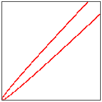
(a) $I=2,K=14$

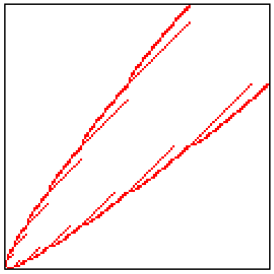
(b) $I=3,K=7$

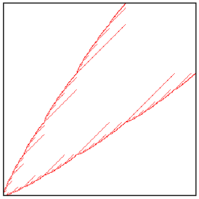
(c) $I=4,K=7$

Figure 12: Support of the transition rate matrix $Q_{K}$ of hyperlattice queuing models (without diagonal entries). The shaded entries correspond to the matrices’ non-zero entries and the white spaces are zero.

We note that the solution to the above balance equations requires a matrix inversion of $Q_{K}$ (or $Q^{\prime}_{K}$), which can become computationally challenging for large matrix sizes. By Lemma 1, the size of $Q_{K}$ can reach a staggering $U_{K}\approx(K+I)^{I}/I!$ (using Stirling’s approximation [19]) even for moderate values of $K$ when the system has $I>2$ servers, presenting a considerable computational hurdle. Fortunately, the sparsity of transition rate matrices (as illustrated in Figure 12) can be leveraged to iteratively find the steady-state distribution using the power method [16], by constructing a probability transition matrix of a discrete-time Markov chain through uniformization of the original continuous-time Markov chain. Let $\mathbb{I}$ represent the identity matrix and denote the maximum absolute value on the diagonal of the transition rate matrix $Q_{K}$ as $\gamma=\max|q_{uu}|$. By initializing with a vector $\pi_{K}^{(0)}$, we can compute $\pi_{K}^{(t)}=\pi_{K}^{(t-1)}(\mathbb{I}+Q_{K}/\gamma)$ at each iteration $t=1,2,\dots$, until the distance between $\pi_{K}^{(t)}$ and $\pi_{K}^{(t-1)}$ falls below a specified threshold. The convergence of this approach is guaranteed, and the steady-state distribution can be efficiently computed despite the potentially large size of the transition rate matrix.

2.4 Measures of performance

In this section, we explicate two key performance measures for a service system with overlapping service regions, using the proposed hyperlattice queuing model as a means of analysis.

2.4.1 Individual workloads

The workload of server $i$, denoted by $\rho_{i}$, is simply equal to the fraction of time that server $i$ is busy serving calls. Thus $\rho_{i}$ is equal to the sum of the steady-state probabilities on part of the hyperlattice corresponding to $n_{i}>0$, i.e.,

$$\rho_{i}=\sum_{u\in\mathcal{U}}\mathbbm{1}\{u:n_{i}>0,n_{i}\in B_{u}\}\cdot\mathbb{P}\{B_{u}\},$$ (11)

where $\mathbbm{1}$ denotes indicator function and $n_{i}$ represents the status of server $i$ in state $B_{u}$. In practice, because the efficient model estimation derived in Section 2.3 only computes the steady-state probabilities for the states in $\mathcal{U}_{K}$, the workload of server $i$ is numerically approximated by

$$\rho_{i}\approx\sum_{u\in\mathcal{U}_{K}}\mathbbm{1}\{u:n_{i}>0,n_{i}\in B_{u}\}\cdot\mathbb{P}\{B_{u}\}.$$

The individual workloads can be further used to calculate various types of system-wide workload imbalance defined in [13].

2.4.2 Fraction of dispatches

2.4.3 Fraction of dispatches

For the remainder of the system performance characteristics, it is necessary to compute the fraction of dispatches that send a server to each sub-region under its responsibility. We use $\rho_{i,e}$ to represent the fraction of dispatches from sending server $i$ to one of its primary overlapping service regions $\mathcal{O}_{e}$. We have

$$\rho_{i,e}=\begin{cases}\sum_{u\in\mathcal{U}}\eta_{e,u}(i)\lambda_{e}\mathbb{P}\left\{B_{u}\right\}/\lambda,&\text{ (a) }i\in e,\\ 0,&\text{ (b) }i\notin e,\end{cases}$$ (12)

In addition, we use $\rho_{i,i}$ to represent the fraction of dispatches that send the server $i$ to its primary service region $i$, which is consistently equal to $\lambda_{i}/\lambda$ since this region can exclusively be handled by server $i$. We note that $\rho_{i,e}=0$ if $i\notin e$ and $\sum_{i,k}\rho_{i,e}+\sum_{i}\rho_{i,i}=1$. Additionally, in practice, we consider $u\in\mathcal{U}_{K}$ rather than $\mathcal{U}$ in (12) as we only calculate the steady-state probabilities for the first $U_{K}$ states according to Section 2.3.

Remark 2.

The proportion of dispatches can be employed to derive expressions for travel time metrics. As per Larson (1974), these metrics can be obtained similarly. It is important to note that this is based on the assumption that queuing delay will be the predominant factor affecting the server’s response time for each incident.

3 Experiments

3.1 Synthetic results

In this section, we delve into the assessment of the efficacy of the proposed hyperlattice queuing models via synthetic experiments. These experiments employ diverse parameter settings within synthetic service systems to investigate the accuracy of the performance metrics estimated by our models. To embark on this, we first use the hyperlattice queuing model to estimate the steady-state probabilities of the systems by solving the balance equations (4). Based on the solutions, we then calculate summary statistics, including individual workloads and the fraction of dispatches, according to (11) and (12). To validate the accuracy of our model estimations, we also developed a simulation program using simpy [18], a process-based discrete-event simulation framework based on Python. The primary purpose of this simulation program is to provide a ground truth of the queuing dynamics of the system so that we can compare the estimated performance measures from our model with the simulation results. Each simulation generates 1,000 events, and servers are dispatched from mobile positions. If a server is idle, its position is selected from a uniform distribution over its service region. Otherwise, the server departs from the location of the previous call it is responding to. The servers’ travel speed is a constant value $c=10$. Using the simulation results, we can approximate the true individual workload of each server $\rho_{i}$ by calculating the percentage of time that the server is busy, and the true fraction of dispatches $\rho_{i,e}$ (or $\rho_{i,i}$) by calculating the percentage of calls received in region $e$ (or $i$) that have been assigned to server $i$.

The experiments were carried out on a personal laptop equipped with a 12-core CPU and 18 GB of RAM. With the hyper-parameter set to $K=5$, the hyperlattice queuing models are capable of estimating states that collectively account for over $99.7\%$ in cumulative steady-state probability. This provides a close approximation to the system dynamics while keeping the computation time in milliseconds.

3.1.1 Overlapping patrolling

We also test our models on the synthetic systems that allow overlapping patrolling. Specifically, we create a two-server system where the service region is a 100 by 100 square with a single overlapping service region in the middle ($I=2$ and $E=1$), as depicted in Figure 5 (a). We assume that calls are uniformly distributed with an arrival rate of $\lambda=1$ and that the service rate of each server is fixed at $\mu_{i}=1$. Changing the hyperparameters of the system, such as the size of the overlapping region and the dispatch policy, can significantly shift the queuing dynamics. Our numerical experiments suggest that the hyperlattice queuing models can accurately capture intricate queuing dynamics under different hyperparameter settings for such a system.

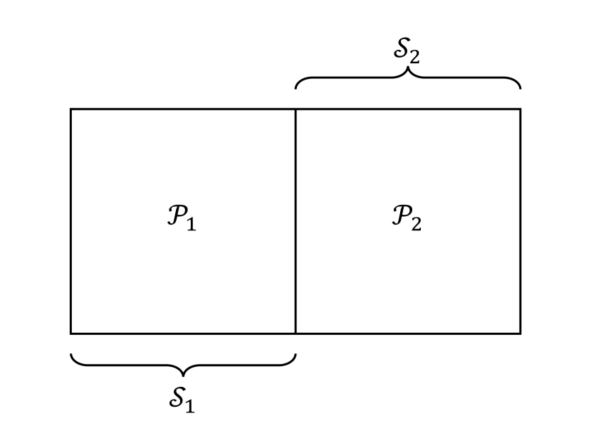
(a) $r=0$

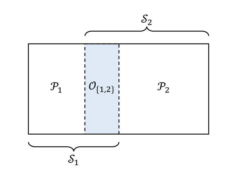
(b) $r=0.4$

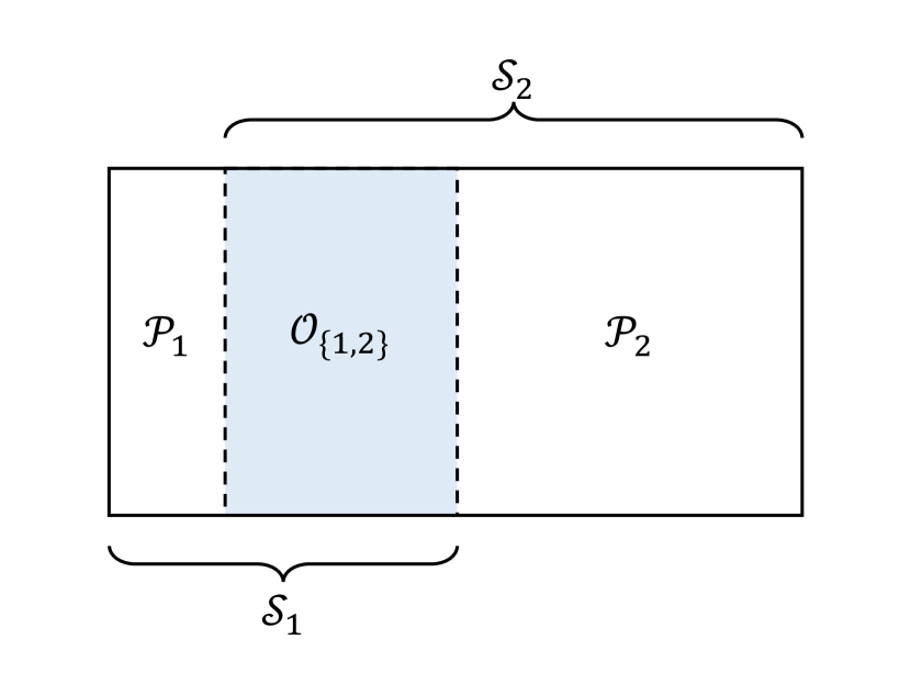
(c) $r=0.7$

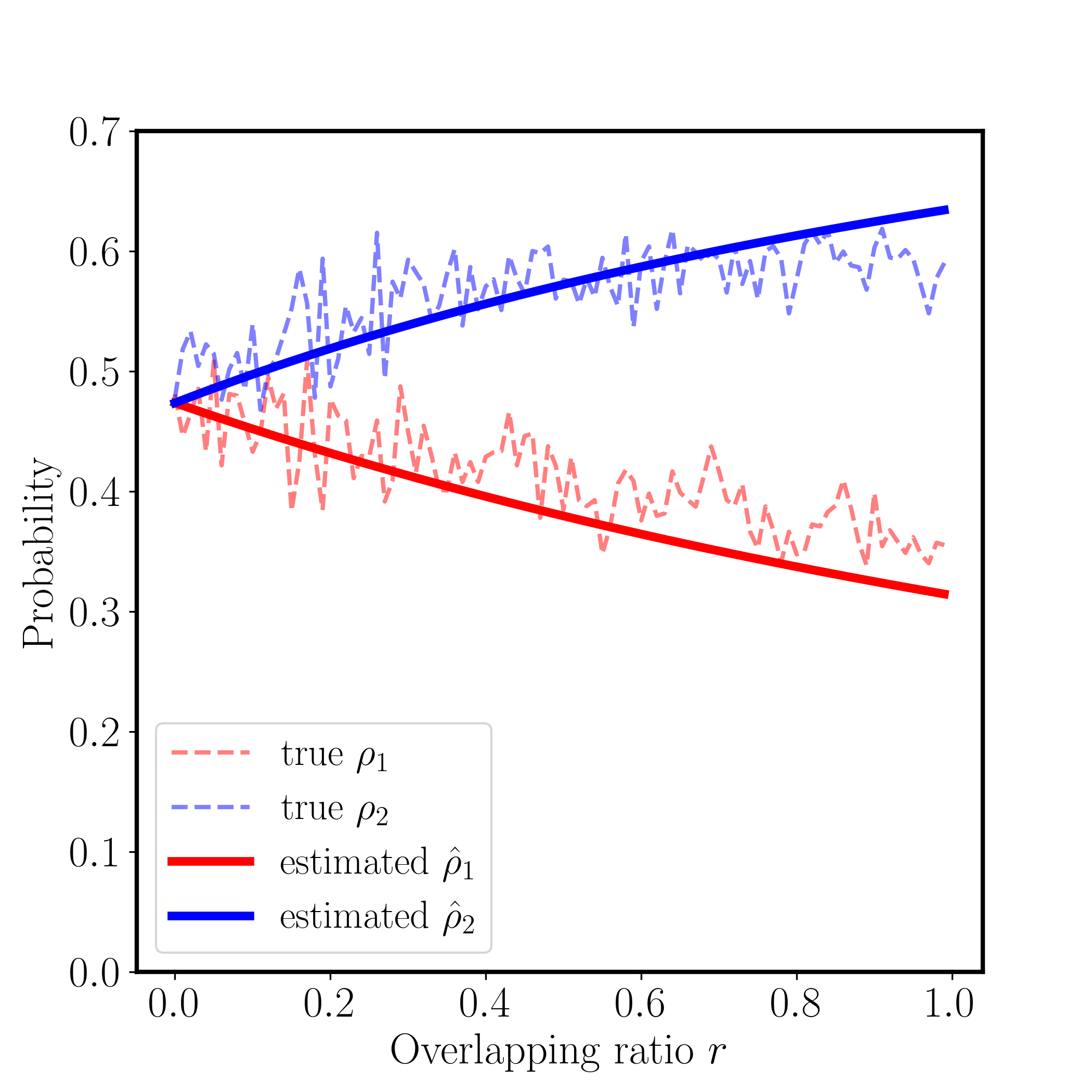
(d) Individual workloads

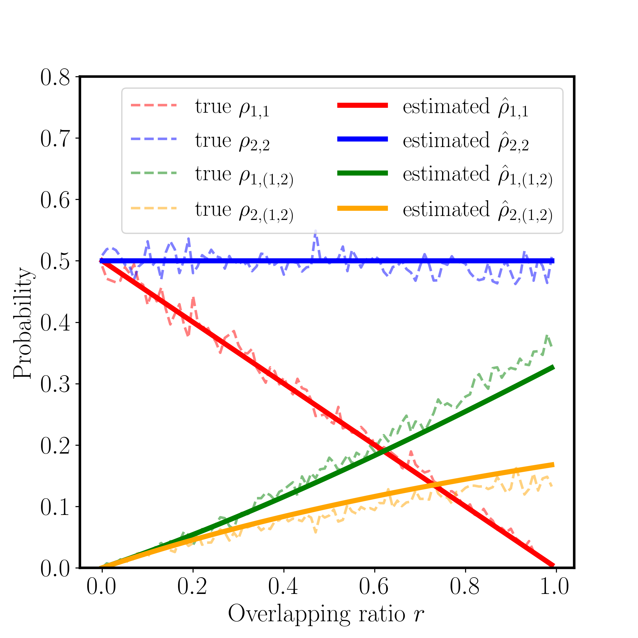
(e) Fraction of dispatches

Figure 13: Synthetic results for two-server systems with varying overlapping ratio $r$. In (a), (b), and (c), the shaded area represents the overlapping region of the system. (d) and (e) show individual workloads $\rho_{i}$ and fraction of dispatches $\rho_{i,(i,j)}$ with varying overlapping ratio $r$. The solid lines represent the estimated performance measures using hyperlattice queuing models, whereas the dashed lines represent the true performance measures obtained from simulation runs.

To examine the impact of overlapping ratio on system dynamics, we first create 100 systems by varying the overlapping ratio $r$. This ratio represents the percentage of the area of the overlapping region with respect to the area of the entire service region of server 1, i.e., $r=|\mathcal{O}_{\{1,2\}}|/(|\mathcal{O}_{\{1,2\}}|+|\mathcal{P}_{1}|)$, as shown in Figure 13 (a-c). We then compare the estimated values of $\rho_{i}$ and $\rho_{i,e}$ to their true values (indicated by dashed lines) in Figure 13 (d) and (e), and find that the estimated values are a good approximation of their true counterparts. Clearly, the workloads of the two servers differ more with an increasing overlapping ratio, enlarging the area server 1 has to cover. Moreover, as the ratio increases, the probability of dispatching either server to the overlap region grows (indicated by green and orange lines), while the probability of sending server 2 to its primary area remains the same (blue line), and the chance of dispatching server 1 decreases (red line). This observation arises from our simplified synthetic setup, where we use a uniform dispatch policy and the dispatch probability to a region directly correlates with its size.

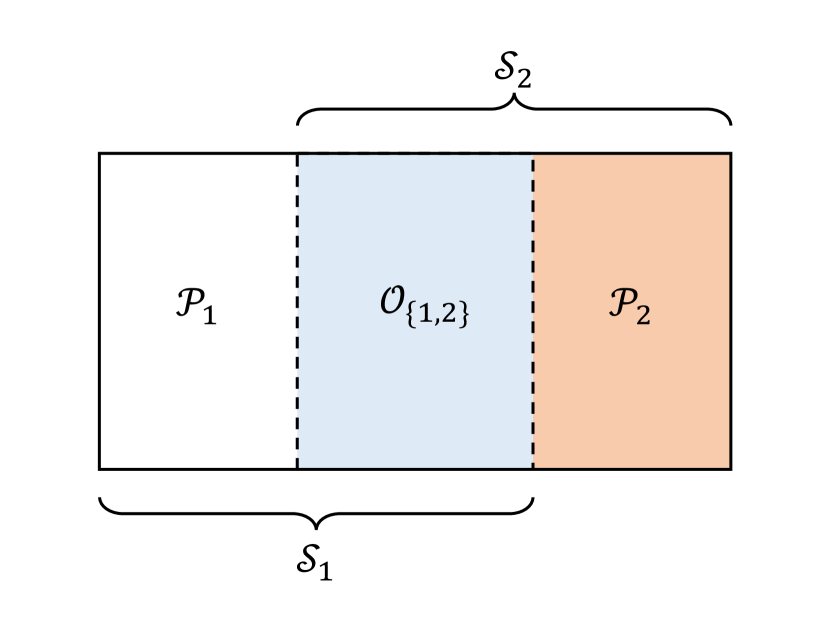
(a) $\eta_{(1,2)}(1)=0$ and $\eta_{(1,2)}(2)=1$

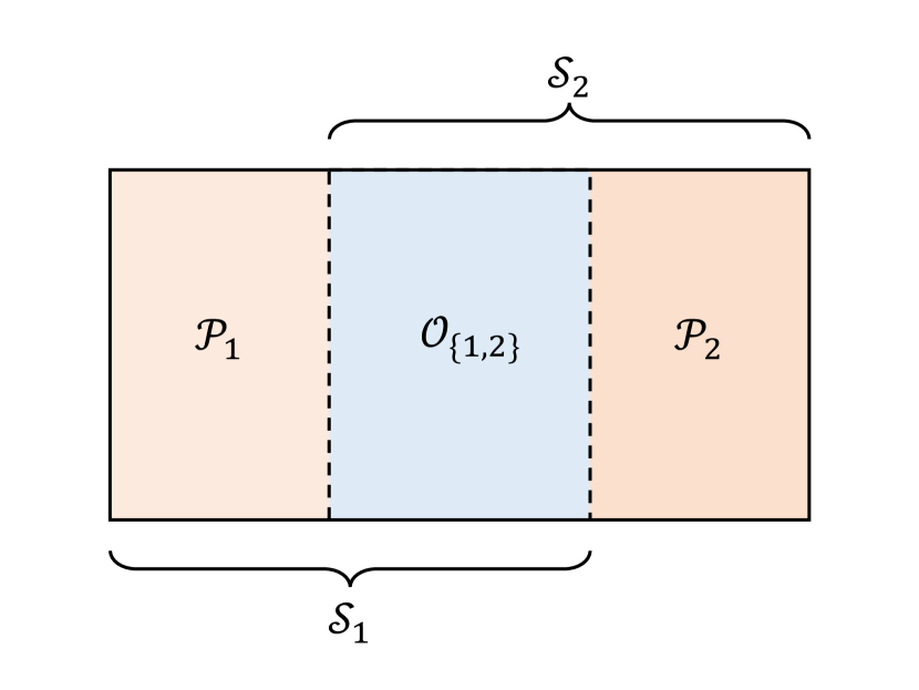
(b) $\eta_{(1,2)}(1)=.4$ and $\eta_{(1,2)}(2)=.6$

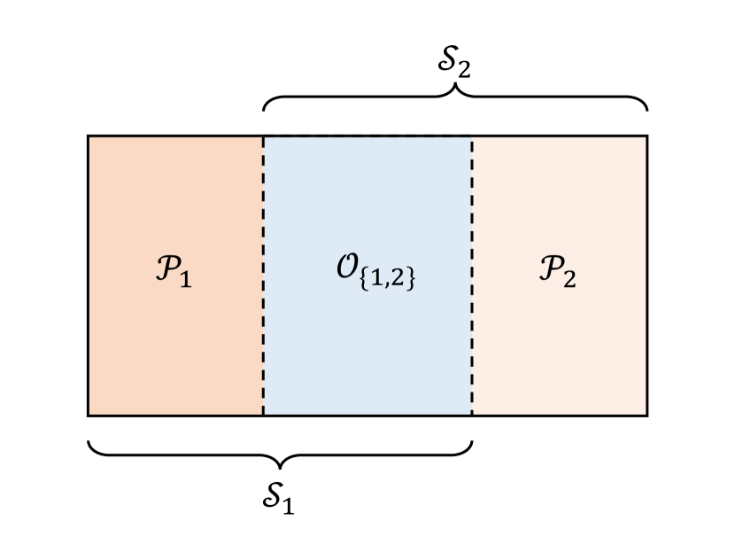
(c) $\eta_{(1,2)}(1)=.7$ and $\eta_{(1,2)}(2)=.3$

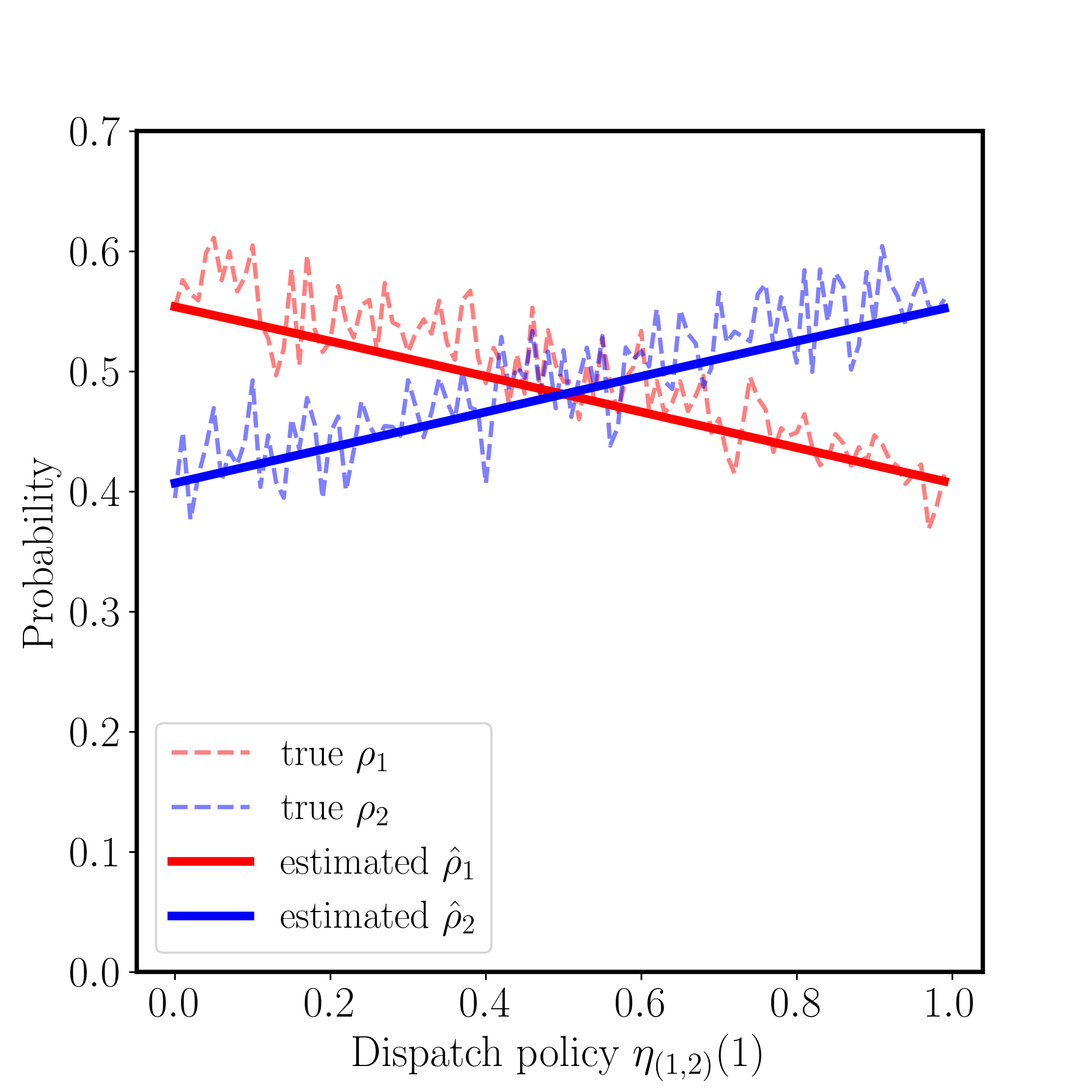
(d) Individual workloads

(e) Fraction of dispatches

Figure 14: Synthetic results for two-server systems with varying dispatch policy $\eta_{(1,2)}(1)$ and $\eta_{(1,2)}(2)$. In (a), (b), and (c), the color depth of region $\mathcal{P}_{1}$ and $\mathcal{P}_{2}$ represents the value of $\eta_{ij}$ and $\eta_{21}$, respectively. (d) and (e) show individual workloads $\rho_{i}$ and fraction of dispatches $\rho_{i,(i,j)}$ with varying dispatch policy $\eta_{(1,2)}(1)$ and $\eta_{(1,2)}(2)$. The solid lines represent the estimated performance measures using hyperlattice queuing models, whereas the dashed lines represent the true performance measures obtained from simulation runs.

Furthermore, we also investigate the impact of dispatch policy by creating another 100 systems with different values of $\eta_{(1,2)}(1)$ and $\eta_{(1,2)}(2)$ (where $\eta_{(1,2)}(1)=1-\eta_{(1,2)}(2)$), while keeping the service regions the same, as shown in Figure 14 (a-c). For the sake of simplicity, we here omit the subscript $u$ in the notation of dispatch policy $\eta_{e}(i),~{}\forall i\in e$ as we assume it doesn’t depend on the state $u$ in this experiment. Figure 14 (d) and (e) show that the estimated $\rho_{i}$ and $\rho_{i,e}$ (indicated by solid lines) are able to closely approximate their true values suggested by the simulation. As we observe, when the dispatch probability for a call from the overlapping region to either server is 0.5, the workload distribution between the two servers is equal, i.e., $\eta_{1,2}(1)=\eta_{1,2}(2)=0.5$.

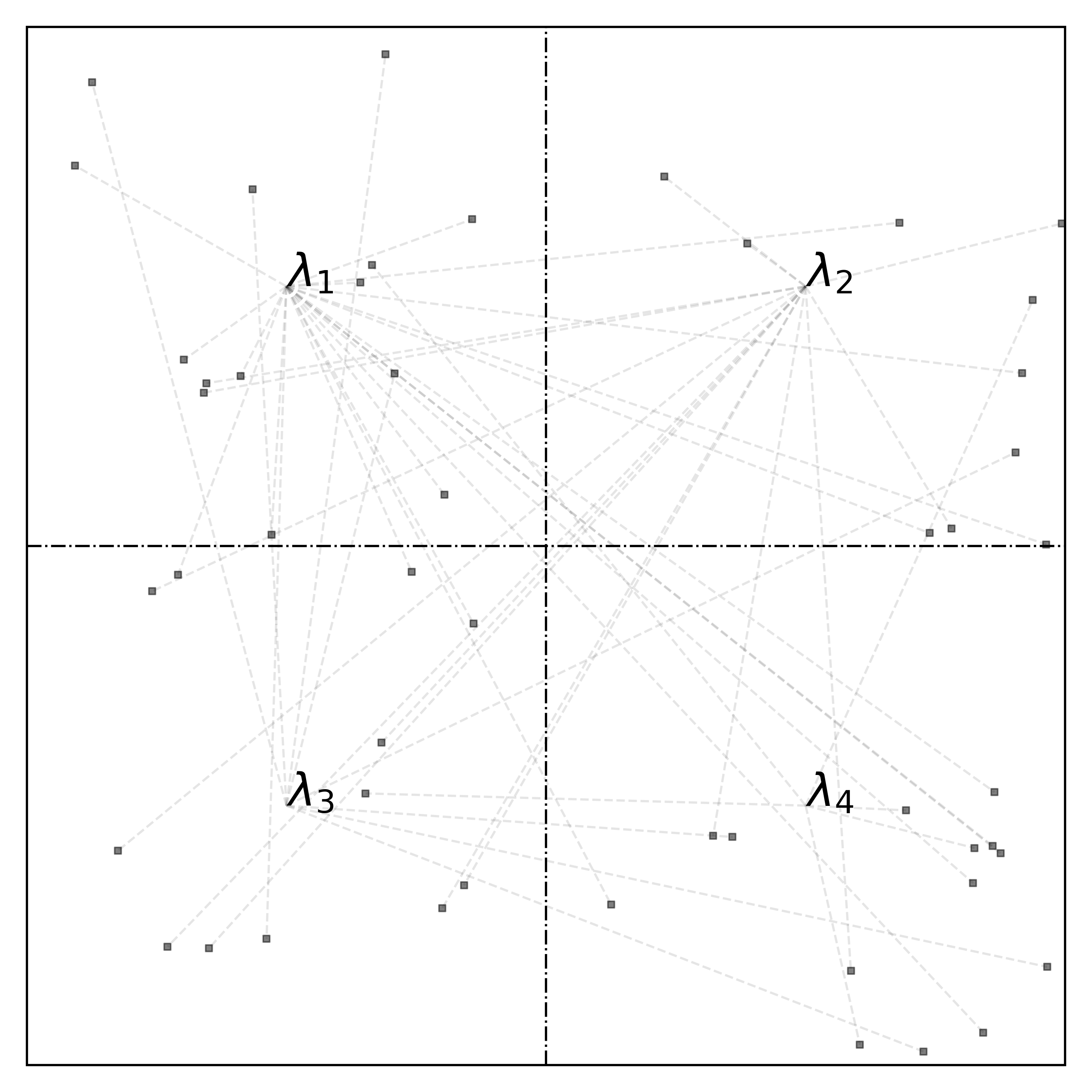
Figure 15: An illustration depicting the experimental setup for the simulation. The dots indicate potential call reception locations, while the dashed lines illustrate the servers’ travel paths during the simulations.

3.1.2 Comparison with Hypercube queue

As discussed in Section 1, a main objective of the hyperlattice model is to extend the classic hypercube queue to capture the high-workload situations more accurately, thus allowing for a detailed analysis of over-saturated systems with queue lengths greater than one. In pursuit of this, we construct a synthetic system subjected to a traditional non-overlapping districting, defined by a $2\times 2$ grid encompassing four identical sub-regions served by their respective servers, as shown in Figure 15. For a meaningful comparison with the hypercube queuing model – where servers can attend to calls from any region if other servers are unavailable – we introduce an overlapping service zone comprised of all four sub-regions. This design ensures no primary service area is designated, granting every server the flexibility to address calls from any sub-region. Furthermore, we operate under the assumption that the call distributions are even across these sub-regions. This results in a call arrival rate of $\lambda/4$ = 1 for each. All servers in this model are consistent in their performance, exhibiting a uniform service rate denoted as $\mu$ = 1. Lastly, we adopt a standardized dispatch policy that is uniformly applied across all servers.

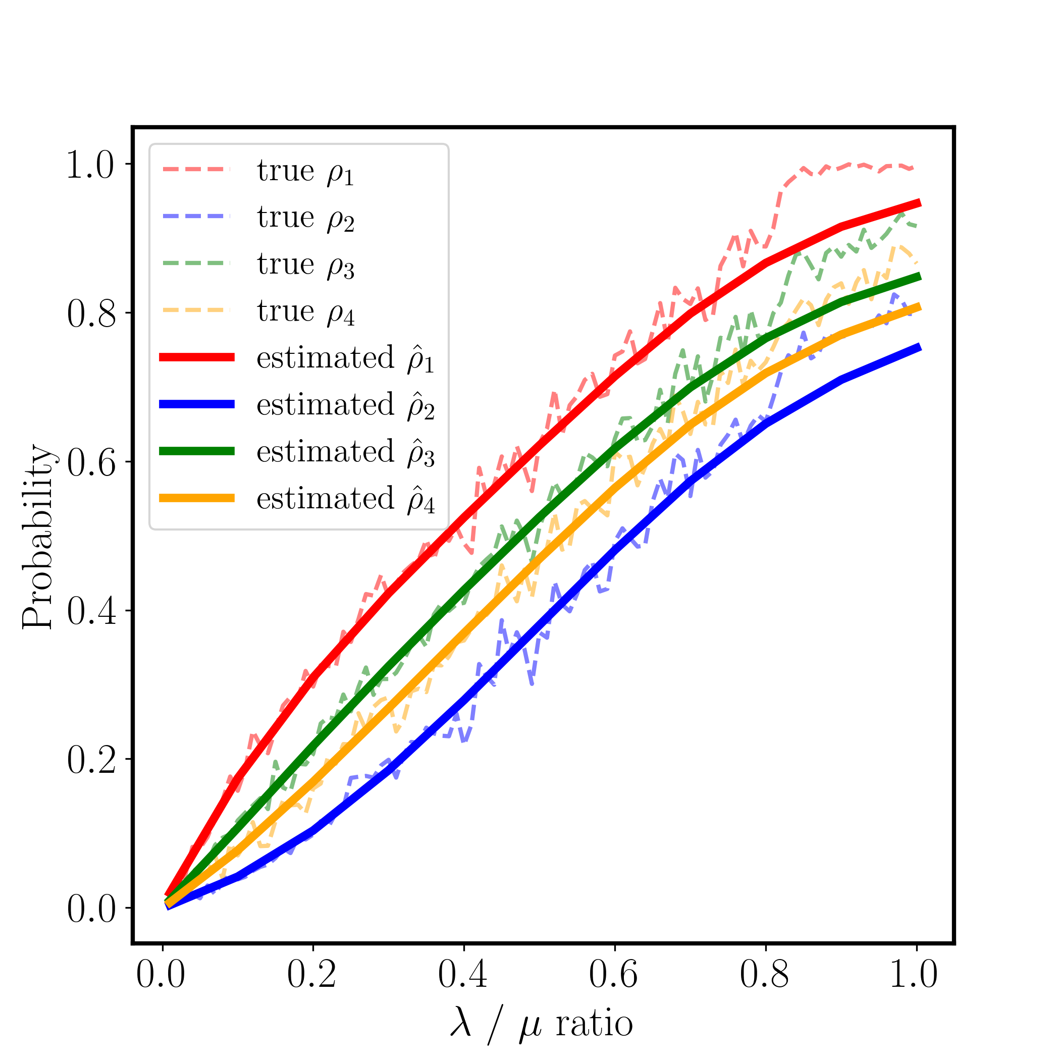
(a) Individual workloads

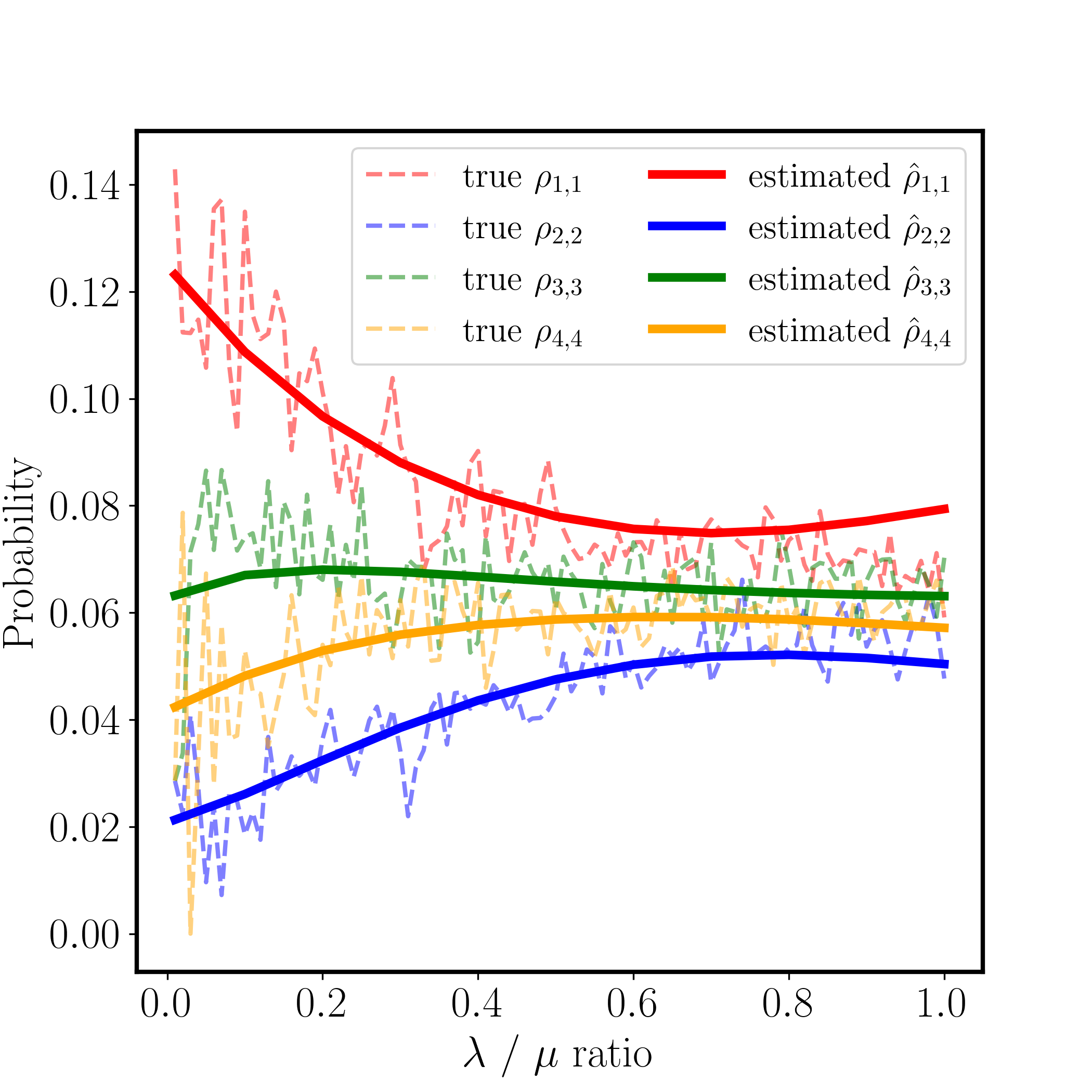
(b) Fraction of dispatches

Figure 16: Synthetic results for four-server systems with varying $\lambda/\mu$ ratio. Figures (a) and (b) show individual workloads $\rho_{i}$ and fraction of dispatches to its own region $\rho_{i,i}$ with varying $\lambda/\mu$ ratio. The solid lines represent the estimated performance measures using hyperlattice queuing models, whereas the dashed lines represent the true performance measures obtained from simulation runs.

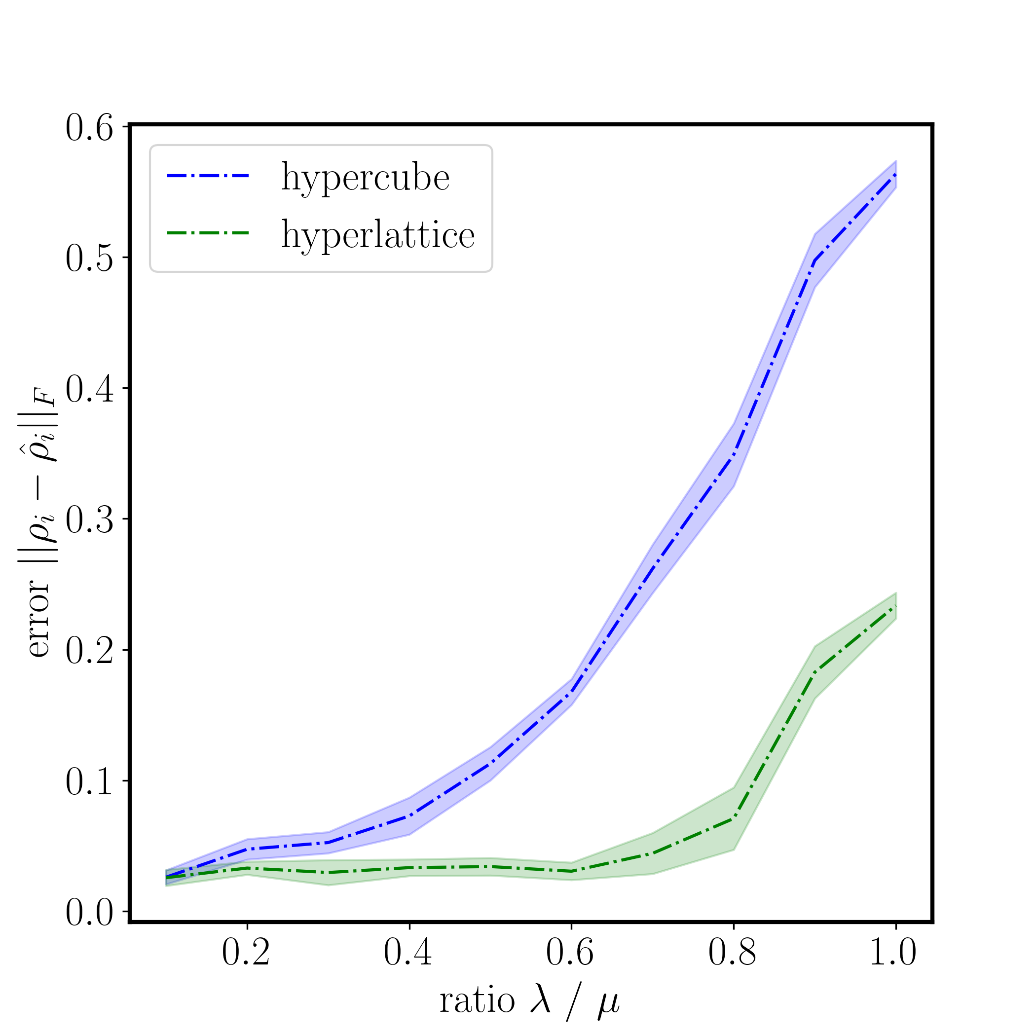
(a) Individual workloads

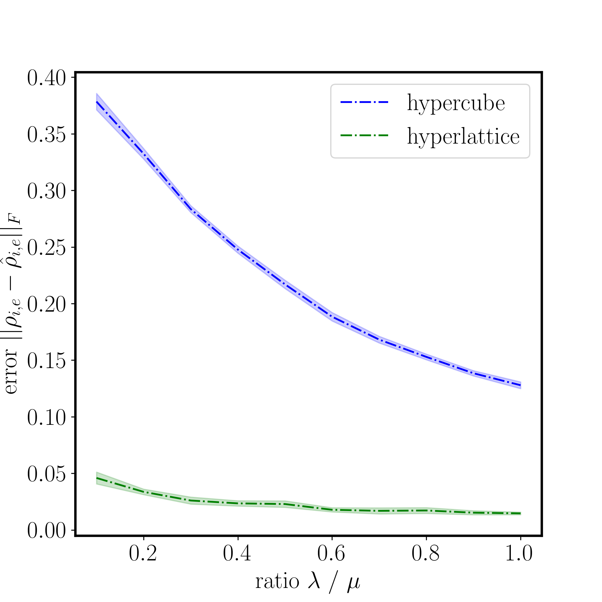
(b) Fraction of dispatches

Figure 17: Frobenius norm of the difference of individual workloads $\rho_{i}$ and fraction of dispatches $\rho_{i,e}$ derived from the hypercube/hyperlattice queuing models and simulation results (denoted as $\hat{\rho}_{i}$ and $\hat{\rho}_{i,e}$) for the systems with varying $\lambda/\mu$ ratio. The dashed lines and the color regions represent the mean and the 95% confidence interval of the norm obtained from 10 simulation runs.

Figure 17 demonstrates the discrepancies in the estimation of individual workloads and dispatch fractions between the hypercube and hyperlattice models. In Figure 17 (a), it is evident that the hypercube model’s effectiveness diminishes substantially as the ratio escalates, whereas our method sustains commendable performance even at higher ratios. This advantage is primarily attributed to the hyperlattice’s capability to account for more detailed dynamics between queues, a feature not present in the hypercube model. Figure 17 (b) further reinforces the superior predictive accuracy of the hyperlattice model in estimating the fraction of dispatches, regardless of the $\lambda/\mu$ ratio. The success is attributed to the harmonized policy adherence between the simulation and that implemented by the hyperlattice model. Furthermore, this dispatch policy demonstrates robustness against fluctuations in the $\lambda/\mu$ ratio. Conversely, the hypercube model, which assumes a shared queue among all servers, fails to capture high-workload dynamics due to its simplified representation of the service process. Moreover, the hypercube model is constrained to a myopic policy (usually only dependent on travel distance) adopting a fixed preference for dispatch that becomes noticeably inadequate at lower $\lambda/\mu$ ratios, leading to a pronounced divergence from simulation results. However, an increase in the ratio sees a shift in the hypercube model towards a homogenous policy, akin to the one employed in our simulation, consequently reducing the gap in estimation accuracy. Such shift underscores the limitations in the hypercube model, demonstrating its restricted adaptability to different scenarios.

3.2 Case study: Police Redistricting in Atlanta, GA

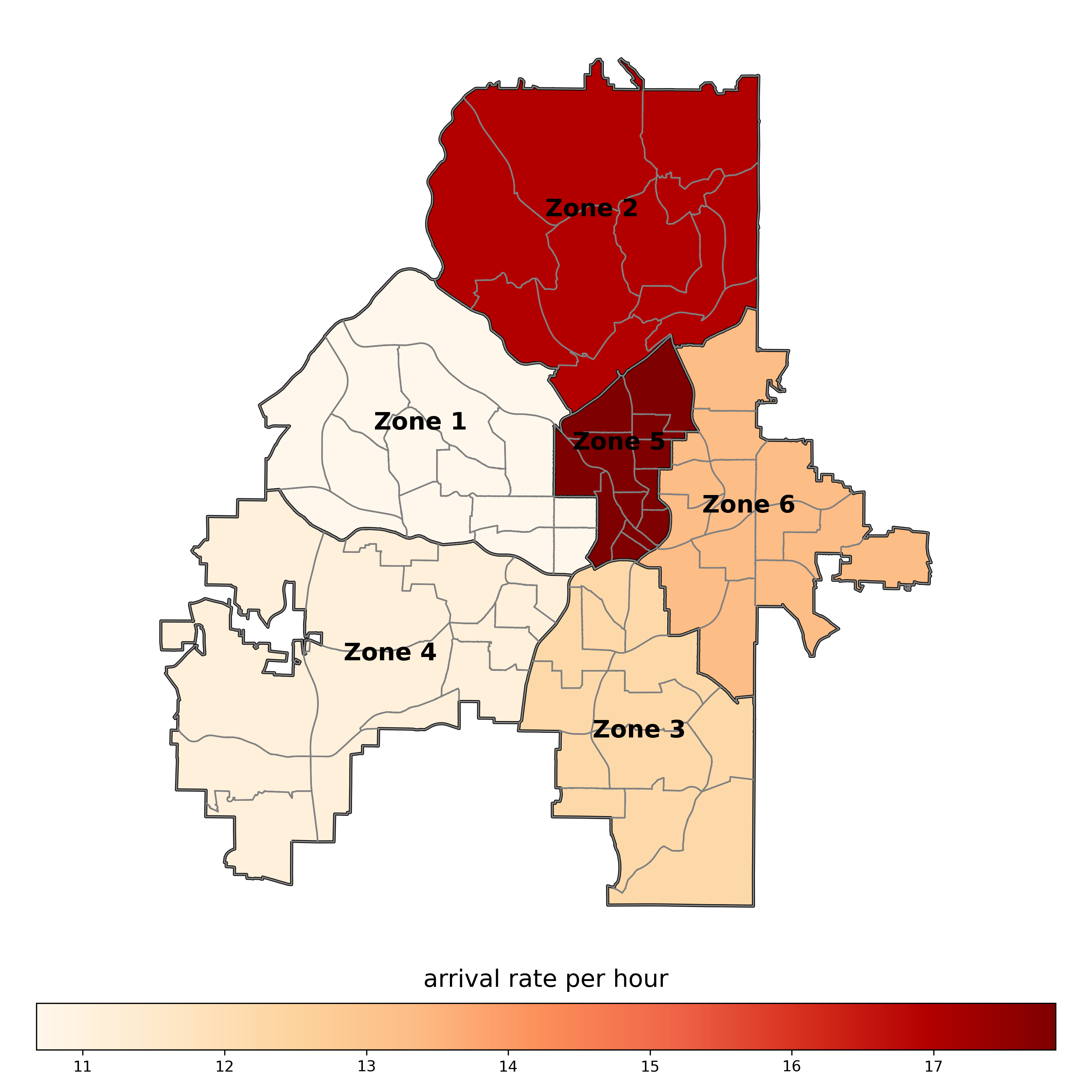
(a) Police zones in Atlanta

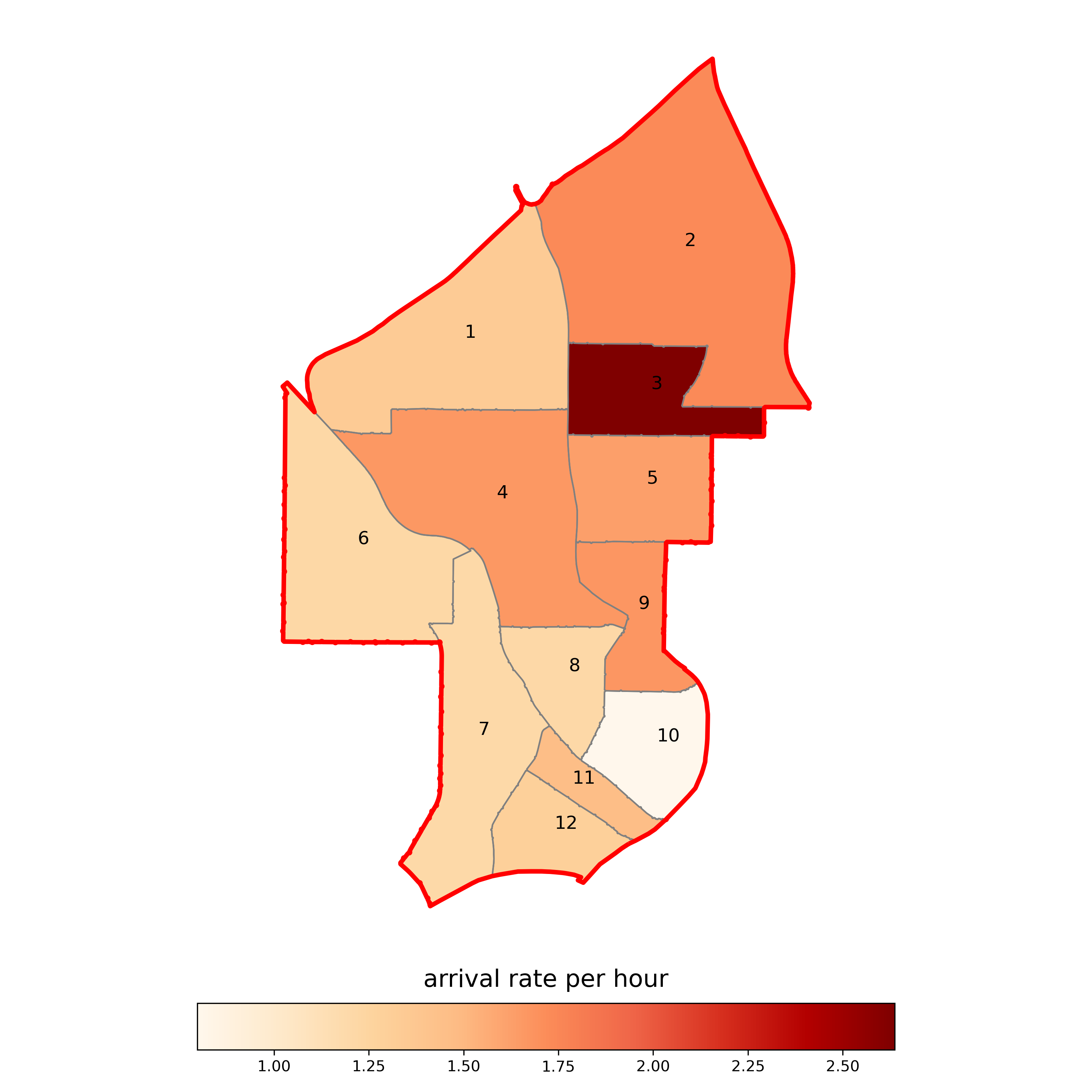
(b) Zone 5

Figure 18: Figure (a) presents a comprehensive map delineating the various police zones in Atlanta, Georgia, while Figure (b) specifically focuses on Zone 5. The intensity of color shading directly corresponds to the frequency of police call arrivals, providing a visual representation of call distribution across the zones.

In this section, we present a case study focusing on the police redistricting problem within Atlanta, Georgia. Figure 18 illustrates the various police zones of the city, with a particular emphasis on the intricate beats of Zone 5. Ideally, each beat would be served by a dedicated police unit, ensuring a focused response within its boundaries. However, this is often not feasible due to a limited number of available police units, primarily attributed to constraints in officer and resource allocation. In instances where certain beats lack a dedicated police unit, units from adjacent beats are required to provide assistance. While such support is permissible among units within the same zone, assistance across zones is explicitly prohibited. The depth of color shading in Figure 18 is a direct representation of the frequency of police call arrivals, quantified by the arrival rate $\lambda$. These rates are estimated based on an analysis of historical 911 calls-for-service data, specifically collected during the years 2021 and 2022, as detailed in the study of [27]. The color reveals that Zone 5 experiences the highest frequency of police calls, approaching an average of 18 calls per hour. As a result, our analysis concentrates on examining potential overlapping districting plans specific to the beats in Zone 5. A key performance metric under consideration is the standard deviation of the individual workloads, as previously discussed in Section 2.4.1. By chosing the hyper-parameter $K=4$, this hyperlattice queuing model can be computed at approximately 10 seconds and estimate the states with a total steady-state probability exceeding $99.9\%$.

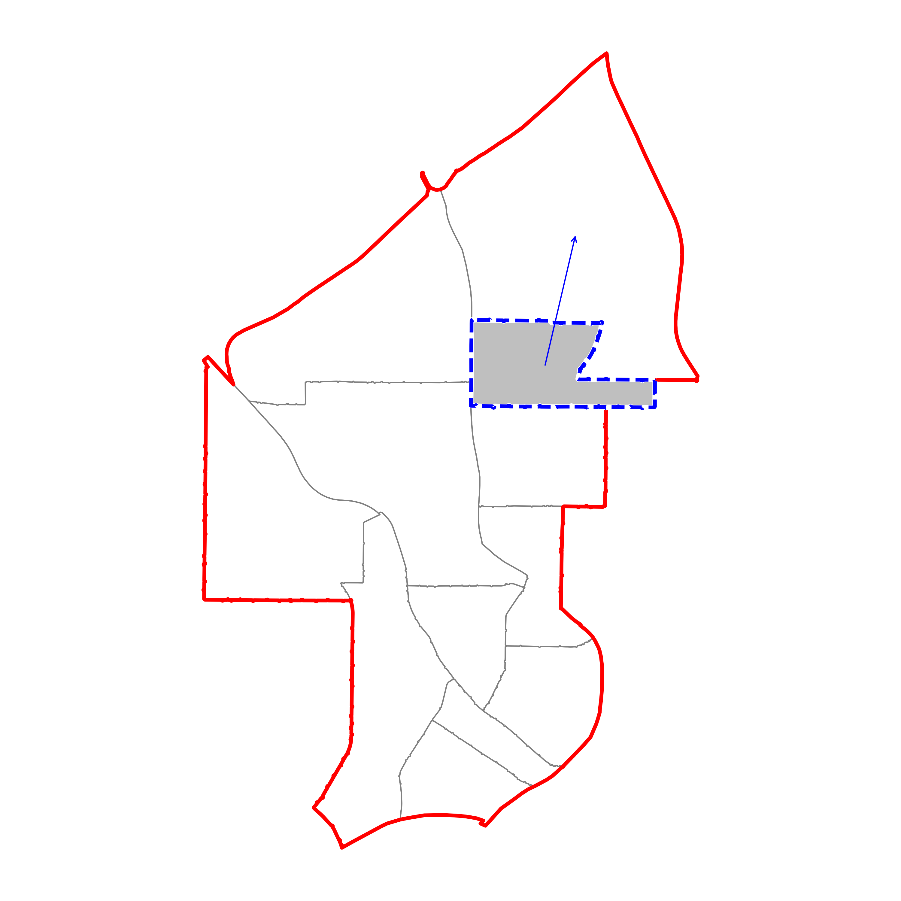
(a) $\sigma$ = 0.13

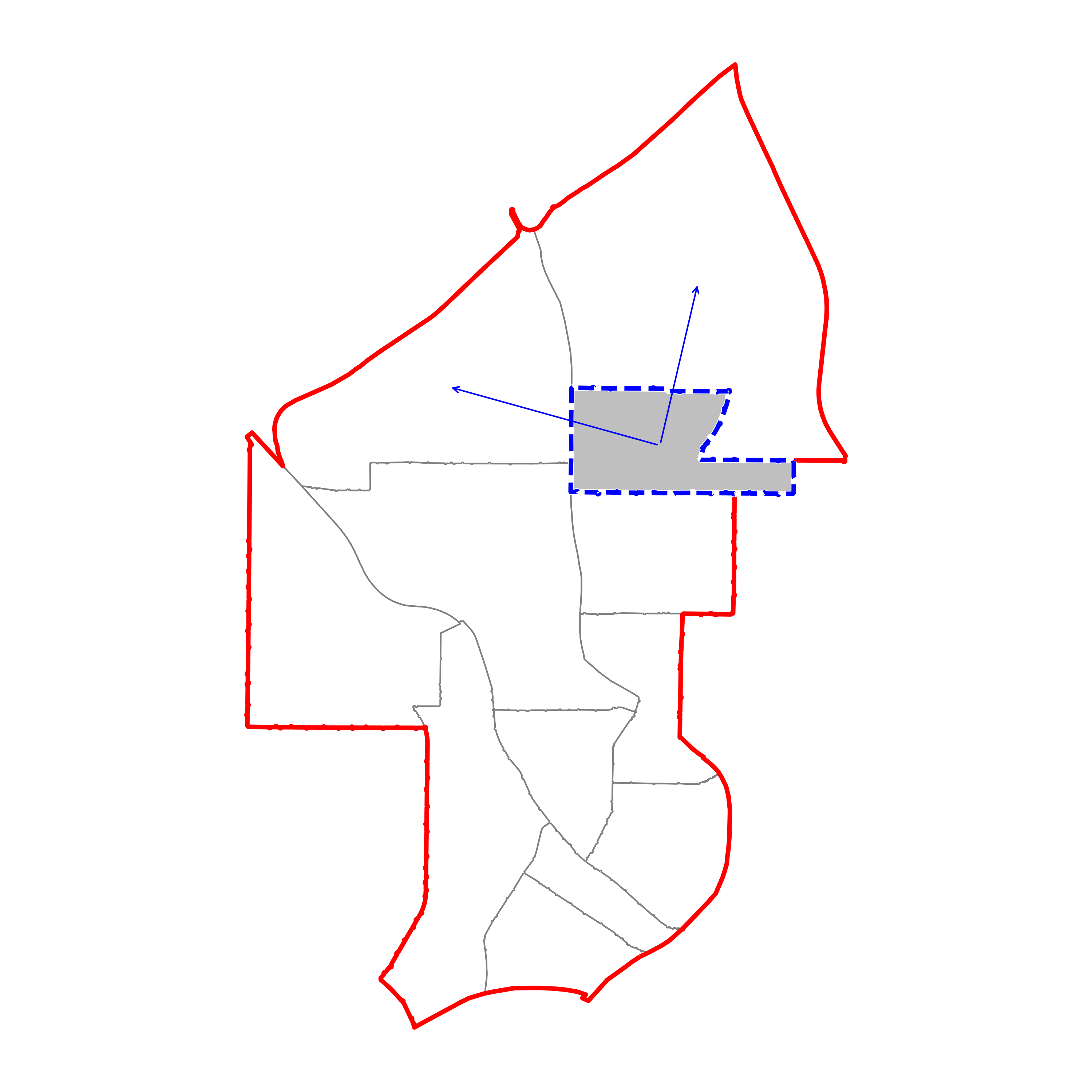
(b) $\sigma$ = 0.11

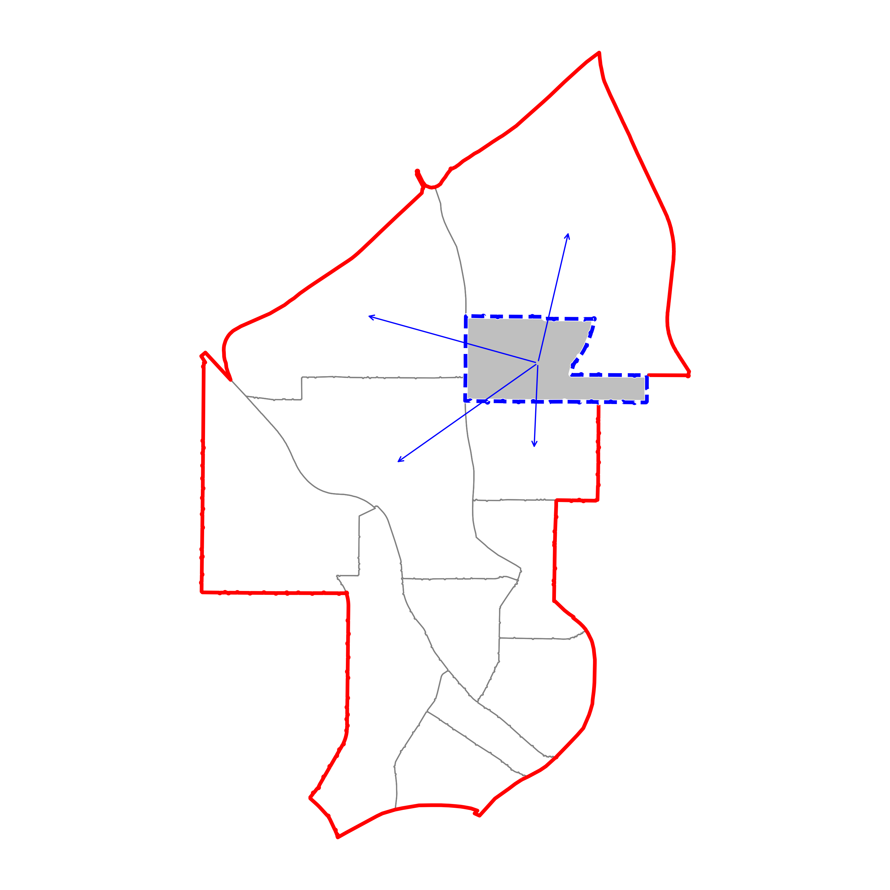
(c) $\sigma$ = 0.08

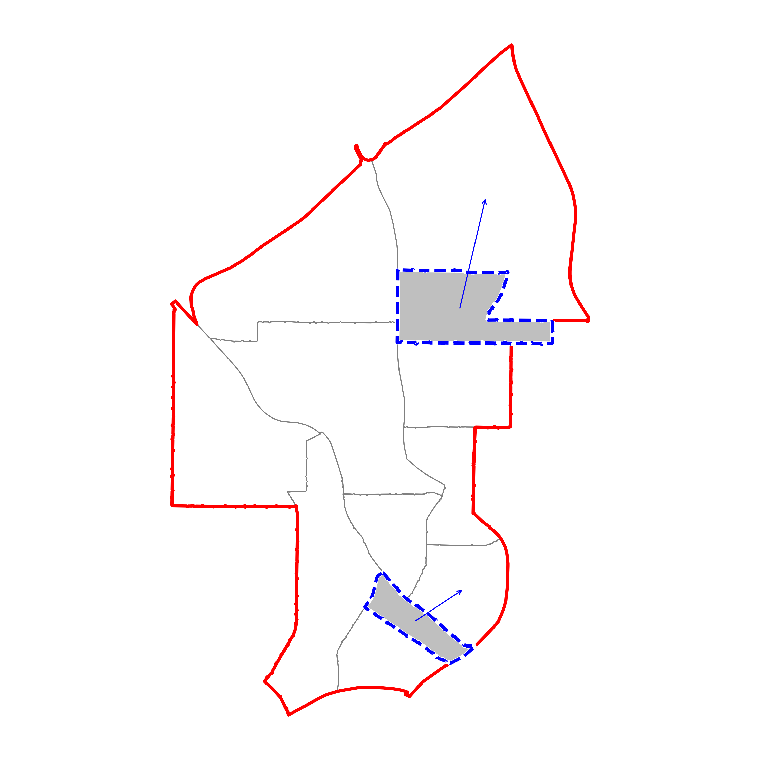
(d) $\sigma$ = 0.13

(e) $\sigma$ = 0.10

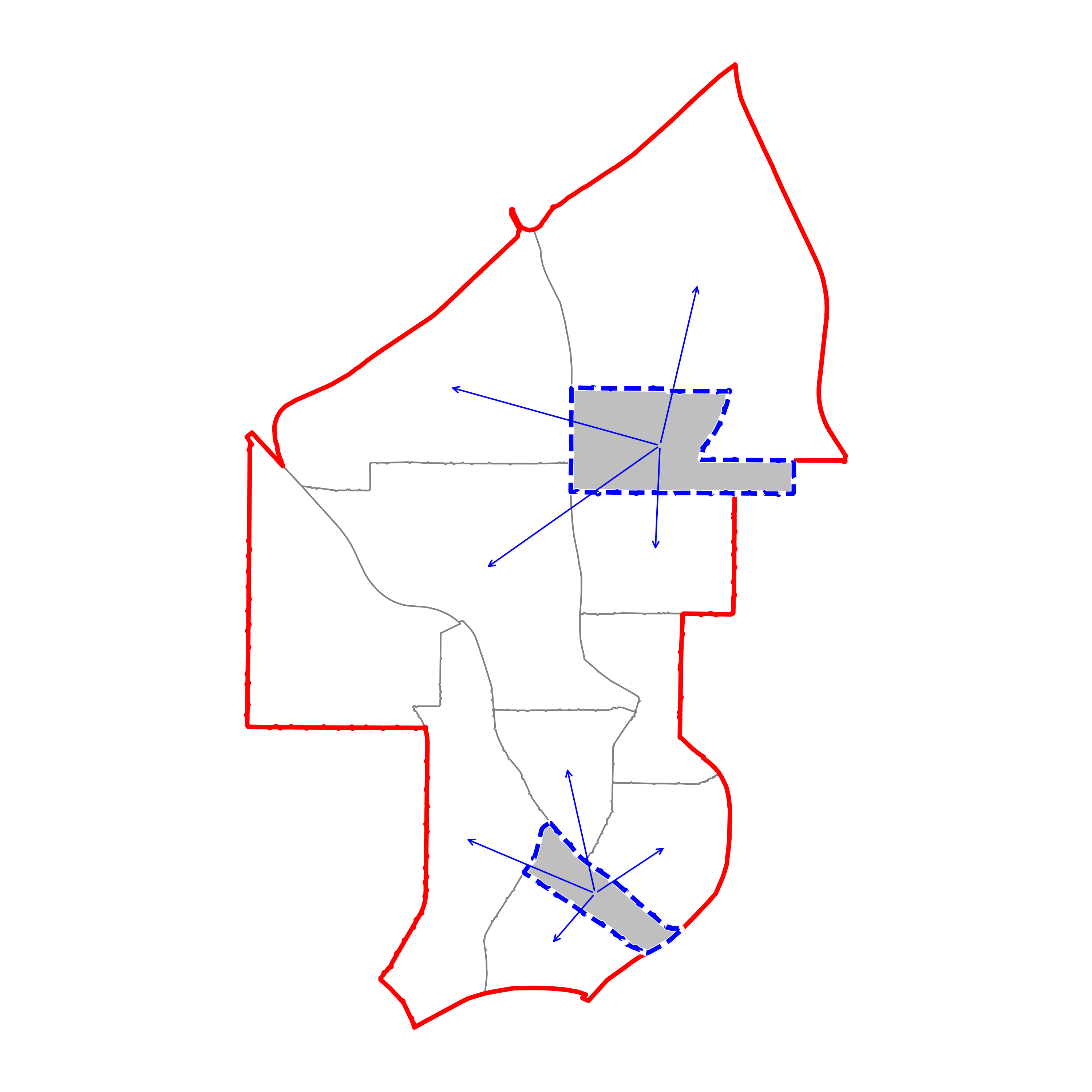
(f) $\sigma$ = 0.06

Figure 19: An illustrative example showing different districting plans for Zone 5 in Atlanta. Gray lines represent the basic geographical units patrolled by the police, red lines outline the districting plans. In the map, regions shaded in grey with dashed blue lines represent beats without a dedicated police unit. The presence of blue arrows originating from these beats signifies that their policing needs are addressed by units from adjacent beats.

In Figure 19, we measure the standard deviation of the individual workloads for different overlapping districting plans using the hyperlattice model with $K=4$, denoted as $\sigma$. Panels (a), (b), and (c) display a scenario where a single beat lacks a dedicated police unit. Specifically, in panel (a), the districting plan is non-overlapping since the policing requirements of this unassigned beat are exclusively managed by a single adjacent beat. In panels (b) and (c), we display different overlapping districting plans by varying the number of overlapping beats. In these configurations, the standard deviations of workload are notably reduced, measured at $0.11$ and $0.08$ respectively, demonstrating the impact of overlapping districts on workload distribution uniformity. Panels (d), (e), and (f) depict scenarios wherein two beats operate without dedicated police units. Notably, panel (f) demonstrates a further reduction in workload standard deviation compared to panel (c), measured at $0.06$, attributable to an additional beat being serviced by the overlapping police units from its neighbors.

Table 3: Workload allocation among police units across beats under various districting plans.

Plan	Beats with Police Unit												$\sigma$
	1	2	3	4	5	6	7	8	9	10	11	12
a	0.28	0.63	-	0.19	0.27	0.19	0.19	0.26	0.27	0.23	0.13	0.21	0.13
b	0.51	0.46	-	0.21	0.28	0.21	0.20	0.28	0.28	0.25	0.14	0.22	0.11
c	0.41	0.35	-	0.33	0.40	0.21	0.21	0.28	0.29	0.25	0.14	0.22	0.08
d	0.27	0.63	-	0.19	0.26	0.19	0.19	0.26	0.26	0.36	-	0.20	0.13
e	0.51	0.46	-	0.20	0.28	0.21	0.20	0.34	0.28	0.32	-	0.22	0.10
f	0.41	0.35	-	0.33	0.40	0.21	0.24	0.31	0.29	0.29	-	0.26	0.06
g	0.29	0.23	0.45	0.21	0.28	0.21	0.20	0.28	0.28	0.25	0.13	0.22	0.07

In Table 3, we record the workload allocation among police units across beats under different districting plans. Plans (a) – (f) align with corresponding panels in Figure 19. Plan (g) depicts an independent scenario where each beat is serviced by a dedicated police unit with non-overlapping districts. It is noteworthy that the total number of police units varies by districting plan, with plans (a) – (c) utilizing 11 units, plans (d) – (f) utilizing 10 units, and plan (g) utilizing all 12 units. We observe that plan (f) exhibits a lower standard deviation in workload compared to plan (g), despite the latter having two additional police units.

The case study also provides valuable managerial insights for addressing the police redistricting problem. It shows that deploying a larger number of police units does not necessarily equate to more effective policing. For instance, plan (f) with 10 units had a lower workload standard deviation compared to plan (g) with 12 units. This suggests that the utilization of overlapping police beats, as opposed to a rigid, non-overlapping structure, can significantly enhance the efficiency of resource allocation. The overlapping districting approach allows for a more flexible and dynamic response to varying call frequencies, especially in high-demand areas like Zone 5 in Atlanta or other cities that face similar challenges.

4 Discussions

This paper presents a novel generalized hypercube queuing model that captures the detailed queuing dynamics of each server in a system. We demonstrate the model’s versatility by applying it to analyze overlapping patrols. Our Markov model employs a hyperlattice to represent an extensive state space, where each vertex corresponds to an integer-valued vector. The transition rate matrix is highly sparse, permitting transitions between vectors with an $\ell_{1}$ distance difference of 1. To enhance computational tractability, we introduce an efficient state aggregation technique that connects our model to a general birth-and-death process with state-dependent rates. This simplifies the detailed balancing equations into a significantly smaller linear system of equations, facilitating the efficient calculation of steady-state distributions. These distributions are essential for evaluating general performance metrics, as acknowledged in Larson’s seminal work.

We emphasize that akin to the rationale in Larson’s original paper [13], no exact analytical expression exists for the hyperlattice model regarding travel time measures for an infinite-line capacity system. This challenge stems from the server’s position not being chosen based on the call’s received region probability distribution during system saturation periods when the server is dispatched consecutively. Consequently, in practice, we must assume that queuing delay is the primary factor influencing the server’s response time for each call.

Additionally, we highlight that our framework concentrates on a random policy controlled by a set of state-dependent matrices, and it can be extended to more intricate decision-making situations. This generalization would empower us to develop and optimize police dispatching policies that take into account queuing dynamics for more realistic systems. This consideration is particularly relevant since conventional First-Come-First-Served (FCFS) approaches may not be optimally efficient, leaving room for enhancement and optimization. Lastly, despite concentrating on police districting in our paper, the generalized hypercube queuing model can also be used for modeling mobile servers in a broader range of applications.

Appendix A Special case: Two servers sharing an overlapping service region

In this section, we discuss a special case of our framework, where the system only allows at most two servers patrolling an overlapping service region, as illustrated by both Figure 5 (a) and (b).

Because only two servers are allows to patrol an overlapping service region, the system can be described by a regular graph, where edges are defined by a set of two vertices. The overlapping service regions can be represented by a pair of server indices ${i,j}$ and the dispatch policy can be simply redefined as $\eta_{ij}$, which represents the probability of choosing server $i$ in overlapping region $(i,j)$ as $\eta_{ij}$ and we have $\eta_{ij}+\eta_{ji}=1$ for $(i,j)\in\mathcal{E}$. Therefore, the upward transition rate defined in (1) can be specified as follows: For an arbitrary state index $u$, the upward transition rate from $B_{u}$ to $B_{u^{i+}}$ is:

$$q_{uu^{i+}}=\begin{cases}~{}\lambda_{i}+\sum_{j:n_{j}>0,j\neq i}\eta_{ij}\lambda_{(i,j)},&~{}(a)~{}n_{i}>0,\\ ~{}\lambda_{i}+\sum_{j:n_{j}=0,j\neq i}\eta_{ij}\lambda_{(i,j)}+\sum_{j:n_{j}>0}\lambda_{(i,j)},&~{}(b)~{}n_{i}=0,\end{cases}$$ (13)

where (a) represents the rate of assigning a new call to a busy server, while (b) represents the rate of assigning a new call to an idle server.

The following argument justifies the above definition. First, for an arbitrary server $i$, it must respond to a call received in its primary service region $i$. Secondly, we assume a new call will be randomly assigned to a server when both servers are available or there is no available server. Then server $i$ needs to randomly respond to a call in two scenarios: (a) If server $i$ is already busy and the new call is received in the overlapping service region $(i,j)$ when server $j$ is also busy, with the determination made based on the probability $\eta_{ij}$; (b) If server $i$ is currently idle and the new call is received in the overlapping service region $(i,j)$, and server $j$ is either busy or idle (with the determination made based on the probability $\eta_{ij}$).

This redesigned definition assures that Proposition 2 retains its validity. The proof can be found below:

Proof.

To begin with, we define $\bar{\lambda}(B_{u})\coloneqq\sum_{i\in\mathcal{I}}q_{uu^{i+}}$ as the total sum of upward transition rates originating from an arbitrary state $B_{u}$. Given the upward transition rates that leave state $B_{u}$ defined in (1), we have

$$\bar{\lambda}(B_{u})= ~{}\sum_{i\in\mathcal{I}}q_{uu^{i+}}$$

$$= ~{}\sum_{i:n_{i}>0}q_{uu^{i+}}+\sum_{i:n_{i}=0}q_{uu^{i+}}$$

$$= ~{}\sum_{i:n_{i}>0}\left(\lambda_{i}+\sum_{j:n_{j}>0,j\neq i}\eta_{ij}\lambda_{(i,j)}\right)+\sum_{i:n_{i}=0}\left(\lambda_{i}+\sum_{j:n_{j}=0,j\neq i}\eta_{ij}\lambda_{(i,j)}+\sum_{j:n_{j}>0,j\neq i}\lambda_{(i,j)}\right)$$

$$= ~{}\sum_{i:n_{i}>0}\sum_{j:n_{j}>0,j\neq i}\eta_{ij}\lambda_{(i,j)}+\sum_{i:n_{i}=0}\sum_{j:n_{j}=0,j\neq i}\eta_{ij}\lambda_{(i,j)}+\sum_{i:n_{i}=0}\sum_{j:n_{j}>0,j\neq i}\lambda_{(i,j)}+\sum_{i\in\mathcal{I}}\lambda_{i}$$

$$= ~{}\sum_{i\in\mathcal{I}}\sum_{j\in\mathcal{I}}\mathbbm{1}\{j\neq i\}\left(\mathbbm{1}\{n_{i}>0,n_{j}>0\}\eta_{ij}\lambda_{(i,j)}+\mathbbm{1}\{n_{i}=0,n_{j}=0\}\eta_{ij}\lambda_{(i,j)}\right)$$

$$+ ~{}\sum_{i\in\mathcal{I}}\sum_{j\in\mathcal{I}}\mathbbm{1}\{j\neq i\}\mathbbm{1}\{n_{i}=0,n_{j}>0\}\lambda_{(i,j)}+\sum_{i\in\mathcal{I}}\lambda_{i}$$

$$\overset{(i)}{=} ~{}\sum_{(i,j)\in\mathcal{E}}\left(\mathbbm{1}\{n_{i}>0,n_{j}>0\}\lambda_{(i,j)}+\mathbbm{1}\{n_{i}=0,n_{j}=0\}\lambda_{(i,j)}\right)$$

$$+ ~{}\sum_{i\in\mathcal{I}}\sum_{j\in\mathcal{I}}\mathbbm{1}\{j\neq i\}\mathbbm{1}\{n_{i}=0,n_{j}>0\}\lambda_{(i,j)}+\sum_{i\in\mathcal{I}}\lambda_{i}$$

$$\overset{(ii)}{=} ~{}\sum_{(i,j)\in\mathcal{E}}\left(\mathbbm{1}\{n_{i}>0,n_{j}>0\}\lambda_{(i,j)}+\mathbbm{1}\{n_{i}=0,n_{j}=0\}\lambda_{(i,j)}\right)$$

$$+ ~{}\sum_{(i,j)\in\mathcal{E}}\left(\mathbbm{1}\{n_{i}=0,n_{j}>0\}\lambda_{(i,j)}+\mathbbm{1}\{n_{i}>0,n_{j}=0\}\lambda_{(i,j)}\right)+\sum_{i\in\mathcal{I}}\lambda_{i}$$

$$= \sum_{(i,j)\in\mathcal{E}}\lambda_{(i,j)}+\sum_{i\in\mathcal{I}}\lambda_{i}$$

$$= ~{}\lambda,$$

where the equation $(i)$ holds due to $\eta_{ij}+\eta_{ji}=1$ and the equality $(ii)$ also holds because $\lambda_{(i,j)}=\lambda_{(j,i)}$. Hence, the sum of all upward transition rates leaving any given state is constantly $\lambda$.

Now the birth rate of the aggregated state $N_{k},~{}k\geq 0$ can be obtained by multiplying $\bar{\lambda}(B_{u})$ by the number of states that are part of $N_{k}$, which is equivalent to $\binom{k+I-1}{I-1}$. It is also evident that the total of all downward transition rates leading to an arbitrary state is $\sum_{i\in\mathcal{I}}\mu_{i}$, which is equal to $\mu$. Consequently, we can obtain the death rate of $N_{k},~{}k\geq 1$ similarly by multiplying the total service rate $\mu$ by the number of states included in $N_{k}$. ∎

References

- [1] Ivo Adan, Robert D Foley, and David R McDonald. Exact asymptotics for the stationary distribution of a markov chain: A production model. Queueing Systems, 62(4):311–344, 2009.
- [2] Sardar Ansari, Laura Albert McLay, and Maria E Mayorga. A maximum expected covering problem for district design. Transportation Science, 51(1):376–390, 2017.
- [3] Sardar Ansari, Soovin Yoon, and Laura A Albert. An approximate hypercube model for public service systems with co-located servers and multiple response. Transportation Research Part E: Logistics and Transportation Review, 103:143–157, 2017.
- [4] Deepak Bammi. Allocation of police beats to patrol units to minimize response time to calls for service. Computers & Operations Research, 2(1):1–12, 1975.
- [5] Caio Vitor Beojone, Regiane Máximo de Souza, and Ana Paula Iannoni. An efficient exact hypercube model with fully dedicated servers. Transportation Science, 55(1):222–237, 2021.
- [6] Alain Bretto. Hypergraph theory. An introduction. Mathematical Engineering. Cham: Springer, 1, 2013.
- [7] Ciara Cummings. Metro police agencies face double-digit staffing shortages. https://www.atlantanewsfirst.com/2022/06/15/metro-police-agencies-face-double-digit-staffing-shortages/, 2022. (Accessed on 04/04/2023).
- [8] J. G. Dai and J. Michael Harrison. Processing Networks: Fluid Models and Stability. Cambridge University Press, 2020.
- [9] Regiane Máximo de Souza, Reinaldo Morabito, Fernando Y Chiyoshi, and Ana Paula Iannoni. Incorporating priorities for waiting customers in the hypercube queuing model with application to an emergency medical service system in brazil. European journal of operational research, 242(1):274–285, 2015.
- [10] Philippe Flajolet and Robert Sedgewick. Analytic combinatorics. cambridge University press, 2009.
- [11] Linda Green. A multiple dispatch queueing model of police patrol operations. Management science, 30(6):653–664, 1984.
- [12] Charles H Jones. Generalized hockey stick identities and -dimensional block walking. Fibonacci Quarterly, 34(3):280–288, 1996.
- [13] Richard C Larson. A hypercube queuing model for facility location and redistricting in urban emergency services. Computers & Operations Research, 1(1):67–95, 1974.
- [14] Richard C Larson and Amedeo R Odoni. Urban Operations Research. Prentice Hall, 1981.
- [15] Reinaldo Morabito, Fernando Chiyoshi, and Roberto D. Galvão. Non-homogeneous servers in emergency medical systems: Practical applications using the hypercube queueing model. Socio-Economic Planning Sciences, 42(4):255–270, 2008.
- [16] Yurii Nesterov and Arkadi Nemirovski. Finding the stationary states of markov chains by iterative methods. Applied Mathematics and Computation, 255:58–65, 2015.
- [17] Chun Peng, Erick Delage, and Jinlin Li. Probabilistic envelope constrained multiperiod stochastic emergency medical services location model and decomposition scheme. Transportation science, 54(6):1471–1494, 2020.
- [18] Spyros Prountzos, Anastasios Matzavinos, and Eleftherios Lampiris. Simpy: Simulation in python. https://simpy.readthedocs.io/, 2021.
- [19] Dan Romik. Stirling’s approximation for : the ultimate short proof? The American Mathematical Monthly, 107(6):556, 2000.
- [20] Renata Algisi Takeda, Joao A Widmer, and Reinaldo Morabito. Analysis of ambulance decentralization in an urban emergency medical service using the hypercube queueing model. Computers & Operations Research, 34(3):727–741, 2007.
- [21] John N Tsitsiklis and Kuang Xu. Flexible queueing architectures. Operations Research, 65(5):1398–1413, 2017.
- [22] Jeremy Visschers, Ivo Adan, and Gideon Weiss. A product form solution to a system with multi-type jobs and multi-type servers. Queueing Systems, 70(3):269–298, 2012.
- [23] Staff Writer. Atlanta-area agency facing critical officer shortage. https://www.policemag.com/command/news/15307675/atlanta-area-agency-facing-critical-officer-shortage, 2023. (Accessed on 04/04/2023).
- [24] Zerui Wu, Ran Liu, and Ershun Pan. Server routing-scheduling problem in distributed queueing system with time-varying demand and queue length control. Transportation Science, 57(5):1209–1230, 2023.
- [25] Soovin Yoon, Laura A Albert, and Veronica M White. A stochastic programming approach for locating and dispatching two types of ambulances. Transportation Science, 55(2):275–296, 2021.
- [26] Shixiang Zhu, Alexander W Bukharin, Le Lu, He Wang, and Yao Xie. Data-driven optimization for police beat design in south fulton, georgia. arXiv preprint arXiv:2004.09660, 2020.
- [27] Shixiang Zhu, He Wang, and Yao Xie. Data-driven optimization for atlanta police-zone design. INFORMS Journal on Applied Analytics, 52(5):412–432, 2022.