Vertical-slice ocean tomography
with seismic waves

Key points

• Seismic T waves at different frequencies sample different parts of the water column.

• Frequency-dependent travel time changes between repeating earthquakes constrain the depth-dependent temperature change between the events.

• These data reveal the vertical structure of temperature anomalies produced by equatorial waves, mesoscale eddies, and decadal warming.

Abstract

Seismically generated sound waves that propagate through the ocean are used to infer temperature anomalies and their vertical structure in the deep East Indian Ocean. These T waves are generated by earthquakes off Sumatra and received by hydrophone stations off Diego Garcia and Cape Leeuwin. Between repeating earthquakes, a T wave’s travel time changes in response to temperature anomalies along the wave’s path. What part of the water column the travel time is sensitive to depends on the frequency of the wave, so measuring travel time changes at a few low frequencies constrains the vertical structure of the inferred temperature anomalies. These measurements reveal anomalies due to equatorial waves, mesoscale eddies, and decadal warming trends. By providing direct constraints on basin-scale averages with dense sampling in time, these data complement previous point measurements that alias local and transient temperature anomalies.

Plain language summary

Taking up almost all of the excess heat trapped on Earth by anthropogenic greenhouse gases, the ocean exerts a key control on our warming climate. Despite progress, tracking that heat remains an observational challenge. This study presents new measurements of ocean warming by making use of sound waves that are generated by earthquakes and propagate long distances through the ocean. These sound waves propagate faster in warmer seawater, so they arrive slightly earlier if warming has occurred. In this study, we measure such changes in arrival time at different frequencies—or pitches—that are sensitive to different parts of the water column, so warming in the upper ocean can be distinguished from warming in the deep ocean.

1 Introduction

The ocean is warming in response to accumulating greenhouse gases in the atmosphere, and its heat capacity dominates the climate system’s thermal inertia. While the warming has been most pronounced in the surface ocean, heat transfer to the deep ocean importantly slows the climate change experienced at the surface [[, e.g.,]]Hansen1984,Gregory2000,Held2010,Kostov2014. [28], for example, estimated from Argo floats that the top $0.5\text{~{}}\mathrm{km}$ of the global ocean warmed at a rate of $5\text{~{}}\mathrm{mK}\text{\,}{\mathrm{yr}}^{-1}$ between 2006 and 2013, whereas the layer between $0.52\text{~{}}\mathrm{km}$ warmed at a rate of $2\text{~{}}\mathrm{mK}\text{\,}{\mathrm{yr}}^{-1}$. Had the heat not been transferred below $0.5\text{~{}}\mathrm{km}$ depth, the top $0.5\text{~{}}\mathrm{km}$ would have warmed more than twice as rapidly (excluding feedbacks with the atmosphere and radiative transfer). It is thus important to constrain the heat transfer to the deep ocean. Because this transfer is achieved by processes that depend on uncertain parameterizations in climate models (the overturning circulation, mesoscale eddies, and diapycnal mixing), strong observational constraints are crucial.

It remains an observational challenge to isolate the small-amplitude and large-scale climate signal in the presence of much larger-amplitude but local fluctuations due to mesoscale eddies, internal waves, and other oceanic transients. To $2\text{~{}}\mathrm{km}$ depth and since the mid-2000s, Argo floats have provided unprecedented coverage of the world ocean. Even with currently about 4000 floats, however, the Argo array still aliases mesoscale eddies, and regional estimates of warming rates remain uncertain [[, e.g.,]Fig. 1a]Wunsch2016,Dushaw2019. Additionally, and maybe more glaringly, Core Argo floats do not sample half of the ocean’s volume: that below $2\text{~{}}\mathrm{km}$ depth. While the Deep Argo array is expanding [[, e.g.,]]Roemmich2019,Johnson2020d, the extant record is short and limited to a few regions. Estimates of temperature change below $2\text{~{}}\mathrm{km}$ rely heavily on sparse hydrographic sections that are sampled about once a decade [[, e.g.,]Fig. 1a]Roemmich1984,Purkey2010,Desbruyeres2016,Desbruyeres2017,Volkov2017. State estimates constrain such changes by combining available observations with an ocean model [[, e.g.,]]Wunsch2007, but the possibility of model error and the lack of an uncertainty estimate make it difficult to assess how reliable such estimates are. For example, [42] inferred widespread cooling of the abyssal ocean using the ECCO (v4r1) state estimate (relative to an assumed and corrected initial state), whereas direct estimates from repeat hydrographic sections tend to indicate a dominance of warming [[, e.g.,]]Purkey2010,Desbruyeres2017. Clearly, better observational constraints are needed.

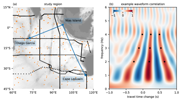
Figure 1: Study region and example measurement of the frequency-dependent travel time change. (a) Locations of the Nias Island earthquakes and the hydrophone receivers at Diego Garcia and Cape Leeuwin. Also shown are the locations of all Argo profiles collected during the ten days following the 2005-03-28 Nias–Simeulue earthquake (orange dots) and the WOCE hydrographic sections (black dots). (b) Frequency-dependent waveform correlation function for the event pair 2005-04-12 09:56:39, 2008-10-11 12:32:32. The black dots indicate measurements for the central maximum as well as the two adjacent maxima that are used for cycle skipping correction (not needed for this pair). An origin time correction of $4.28\text{~{}}\mathrm{s}$ was applied based on the waveforms received at land station PSI.

Recently, [38] demonstrated that sound waves generated by earthquakes, so-called T waves, can be used to constrain basin-scale temperature change in the deep ocean. These measurements are based on the idea of “ocean acoustic tomography,” which was originally proposed by [21] and successfully demonstrated at both planetary [19] and basin scales [34]. T waves propagate faster in warmer water, so changes in the average temperature encountered by these waves can be detected as changes in their travel time. The use of sound waves produced by earthquakes eliminates the need to deploy synthetic sound sources. [38] used the seismic station DGAR on Diego Garcia to receive T waves generated $2900\text{~{}}\mathrm{km}$ away by earthquakes near Nias Island off Sumatra (Fig. 1a). To remove uncertainties in the source location and timing, repeating earthquakes were employed to extract the change in travel time between two events. A key advantage of such acoustic measurements over point measurements is that they intrinsically average the temperature change along the sound waves’ path and therefore suffer much less from spatial aliasing.

In an accompanying manuscript (hereafter referred to as W23), we show that Comprehensive Nuclear-Test-Ban Treaty Organization (CTBTO) hydrophones are more sensitive T-wave receivers than land stations like DGAR, which allows the detection of smaller earthquakes at the CTBTO station H08 off Diego Garcia than is possible with DGAR data. This use of CTBTO data improves the time resolution of the inferred deep-ocean temperature change between Nias Island and Diego Garcia. In W23, we further use Nias Island T-waves received at the CTBTO station H01 off Cape Leeuwin to infer a time series of temperature change averaged along this $4400\text{~{}}\mathrm{km}$ section extending into the extra-tropical ocean (Fig. 1a).

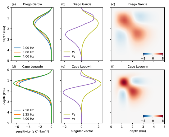
Figure 2: Sensitivity kernels and inference of vertical structure. Shown are (a), (d) the range-averaged sensitivity kernels at different frequencies, (b), (e) the first two singular vectors obtained from these range-averaged sensitivity kernels, and (c), (f) the resolution matrices of the SVD inversion employing the first two singular vectors. All these are shown for the path to Diego Garcia (top row) and that to Cape Leeuwin (bottom row).

Here, we make use of an additional advantage of the crisp arrivals of T waves in CTBTO hydrophone records: that changes in the travel time can be measured reliably at a number of different frequencies (Fig. 1b, Section 2). Because T waves at different frequencies are sensitive to different parts of the water column, this frequency dependence in the travel time change can be used to constrain the vertical structure of the temperature change [[, Fig. 2; cf.,]]Munk1983,Shang1989. This approach is similar to that employed in remote sensing of the atmosphere [[, e.g.,]]Fu2004, except that acoustic rather than electromagnetic waves are used.

A similar vertical-slice tomography scheme has been developed for acoustic measurements with synthetic sources [[, e.g.,]]Munk1979,Munk1982b,Munk1995, but it has not been realized at a basin scale. The sources employed in the Acoustic Thermometry of Ocean Climate (ATOC) experiment had frequencies centered on $75\text{~{}}\mathrm{Hz}$ and were effectively point sources at precisely known locations, allowing for a convenient eigenray description of the propagation from source to receiver. These rays have a known geometry and, under certain circumstances, can be resolved and identified in arrival patterns [33, 35, 1, 34, 37]. Relative changes in the arrival times of different rays can then be used to infer the vertical structure of temperature change, most easily in the range average. For example, the arrival time of steep rays that sample the surface mixed layer undergo a larger seasonal cycle than near-axial rays that are confined to the thermocline and deep ocean. On the bottom-mounted receivers used in ATOC, however, only relatively steep rays could be resolved and identified, and the information on the vertical structure of the temperature field was limited [6, 5].

The propagation and arrival patterns of T waves are more complicated [[, e.g.,]]Okal2008, but information on the vertical structure of the temperature change can still be extracted. Sensitivity kernels quantify how the arrival time changes in response to a temperature perturbation anywhere along the path and anywhere in the water column [[, Fig. 2;]]Wu2020. Consistent with expectations from simplified modal calculations (Fig. LABEL:fig:modekernels), these range-averaged sensitivity kernels shift upward in the water column for increasing frequencies (Fig. 2). A surface-intensified warming, for example, produces a larger reduction in travel time at high frequencies than at low frequencies. We use this frequency dependence to estimate a rough vertical structure of the range-averaged deep temperature anomalies. We find that the inferred structure of the anomalies along the two sections matches expectations based on the dynamics that produce the anomalies and is in general agreement with previous estimates, although the T-wave data tends to show stronger anomalies and more reliably captures perturbations due to mesoscale eddies (Section 3).

2 Inferring vertical structure

The starting point for the inference of vertical structure in the temperature anomalies are the time series of travel time anomalies at a few different low frequencies, constructed from a total of $11\,479$ repeating pairs that arise from $3457$ earthquakes in 2005 to 2018 (Fig. 1b; W23). We choose $2.00\text{~{}}\mathrm{Hz}3.00\text{~{}}\mathrm{Hz}4.00\text{~{}}\mathrm{Hz}$ for the path to Diego Garcia and $2.50\text{~{}}\mathrm{Hz}3.25\text{~{}}\mathrm{Hz}4.00\text{~{}}\mathrm{Hz}$ for the path to Cape Leeuwin. A slightly higher minimum frequency is used for the latter path because $2.00\text{~{}}\mathrm{Hz}$ T waves are less consistently received at Cape Leeuwin than at Diego Garcia. Measurements at higher frequencies are not reliable because the waveform correlation drops markedly beyond $4\text{~{}}\mathrm{Hz}$ (e.g., Fig. 1b). For each frequency, we apply a Gaussian filter with width $0.5\text{~{}}\mathrm{Hz}$ centered on that frequency before calculating the correlation function between the T-wave arrivals of an event pair, as described in W23. How these time series are obtained from measured travel time differences between repeating events is described in LABEL:sec:inversion, and the cycle skipping corrections that are applied to the measurements are described in LABEL:sec:csc.

To turn the time series of travel time anomalies at different frequencies into an estimate of the evolving vertical structure of temperature anomalies, we perform a singular value decomposition (SVD) of the range-integrated sensitivity kernels (Fig. 2). The problem is severely under-determined, so we can only hope to obtain a coarse estimate of the vertical temperature structure. Let $\mathbf{K}$ denote the matrix whose three rows contain the range-integrated sensitivity kernels at the three frequencies, discretized to a $\Delta z=$50\text{~{}}\mathrm{m}$$ grid. Then, at each event time $t$, we would like to invert $\boldsymbol{\tau}(t)=\mathbf{K}\boldsymbol{T}(t)\Delta z$ for $\boldsymbol{T}(t)$, where $\boldsymbol{\tau}(t)$ contains the T-wave travel time anomalies at the three frequencies, and $\boldsymbol{T}(t)$ contains the range-averaged temperature anomaly profiles on the same grid as the kernels. The SVD $\mathbf{K}=\mathbf{U}\boldsymbol{\Lambda}\mathbf{V}^{\mathrm{T}}$ yields the singular values $\lambda_{1}=$2.6\text{~{}}\mathrm{s}\text{\,}{\mathrm{K}}^{-1}\text{\,}{\mathrm{km}}^{-1}$$, $\lambda_{2}=$0.21\text{~{}}\mathrm{s}\text{\,}{\mathrm{K}}^{-1}\text{\,}{\mathrm{km}}^{-1}$$, and $\lambda_{3}=$0.022\text{~{}}\mathrm{s}\text{\,}{\mathrm{K}}^{-1}\text{\,}{\mathrm{km}}^{-1}$$ for the path to Diego Garcia and $\lambda_{1}=$4.6\text{~{}}\mathrm{s}\text{\,}{\mathrm{K}}^{-1}\text{\,}{\mathrm{km}}^{-1}$$, $\lambda_{2}=$0.30\text{~{}}\mathrm{s}\text{\,}{\mathrm{K}}^{-1}\text{\,}{\mathrm{km}}^{-1}$$, and $\lambda_{3}=$0.012\text{~{}}\mathrm{s}\text{\,}{\mathrm{K}}^{-1}\text{\,}{\mathrm{km}}^{-1}$$ for the path to Cape Leeuwin (see LABEL:sec:inversion for details). The rapid decay in the singular values is a result of the similarity of the sensitivity kernels at the chosen frequencies, i.e., their being nearly linearly dependent. Small singular values amplify errors (we only know the estimate $\tilde{\boldsymbol{\tau}}$, not the true $\boldsymbol{\tau}$), so a common trade-off must be made between resolution and precision. We choose to retain the first two singular vectors to obtain coarse vertical resolution with acceptable uncertainty: $\tilde{\boldsymbol{T}}_{2}(t)=h^{-1}\mathbf{V}_{2}\boldsymbol{\Lambda}_{2}\!{}^{-1}\mathbf{U}_{2}\!{}^{\mathrm{T}}\tilde{\boldsymbol{\tau}}(t)$, where $\mathbf{U}_{2}$ and $\mathbf{V}_{2}$ consist of the first two columns of $\mathbf{U}$ and $\mathbf{V}$, respectively, $\boldsymbol{\Lambda}_{2}$ is the diagonal matrix containing $\lambda_{1}$ and $\lambda_{2}$, and $h=$5\text{~{}}\mathrm{km}$$ is a fixed reference depth. The estimate $\tilde{\boldsymbol{T}}_{2}(t)$ is then related to the true temperature field $\boldsymbol{T}(t)$ by $\tilde{\boldsymbol{T}}_{2}(t)=h^{-1}\mathbf{V}_{2}\mathbf{V}_{2}\!{}^{\mathrm{T}}\boldsymbol{T}(t)\Delta z+h^{-1}\mathbf{V}_{2}\boldsymbol{\Lambda}_{2}\!{}^{-1}\mathbf{U}_{2}\!{}^{\mathrm{T}}[\tilde{\boldsymbol{\tau}}(t)-\boldsymbol{\tau}(t)]$. In the absence of errors in $\tilde{\boldsymbol{\tau}}(t)$, the estimate $\tilde{\boldsymbol{T}}_{2}(t)$ is a projection of the true state $\boldsymbol{T}(t)$ onto the first two singular vectors, and the resolution matrix $\mathbf{V}_{2}\mathbf{V}_{2}\!{}^{\mathrm{T}}$ determines to what degree features can be resolved by the available data. For both paths, only features between about $0.53\text{~{}}\mathrm{km}$ depth can be captured, and the depth resolution is no better than about $1\text{~{}}\mathrm{km}$ (Fig. 2). The projection coefficients are estimated from the data as $\tilde{\boldsymbol{c}}_{2}(t)=h^{-1}\mathbf{V}_{2}\!{}^{\mathrm{T}}\tilde{\boldsymbol{T}}_{2}(t)\Delta z=h^{-1}\boldsymbol{\Lambda}_{2}\!{}^{-1}\mathbf{U}_{2}\!{}^{\mathrm{T}}\tilde{\boldsymbol{\tau}}(t)$, with which the reconstructed temperature profile is the linear combination $\tilde{\boldsymbol{T}}_{2}(t)=\mathbf{V}_{2}\tilde{\boldsymbol{c}}_{2}(t)$. (Note that the prior covariances for inferring $\tilde{\boldsymbol{\tau}}(t)$ from the travel time changes between repeating events are chosen such that the three components of $\tilde{\boldsymbol{c}}(t)=h^{-1}\boldsymbol{\Lambda}^{-1}\mathbf{U}^{\mathrm{T}}\tilde{\boldsymbol{\tau}}(t)$ are uncorrelated. Any phase relations between them therefore arise entirely from the data. Details are given in LABEL:sec:inversion.)

Taking this SVD approach to inversion, we feign complete ignorance about the vertical structure of the range-averaged temperature anomalies. The inversion uses neither constraints from the physics that govern the temperature field nor prior information, say from previous measurements or model simulations. In particular, the inversion knows nothing of the typically strong surface intensification of temperature anomalies, which entails that inverted temperature anomalies tend to reach too deep and that upper-ocean anomalies can produce spurious oppositely signed deep anomalies (Fig. LABEL:fig:h08depth, LABEL:fig:h01depth). We nevertheless choose this agnostic approach to illustrate most simply what information is contained in the T-wave data. Future work should combine this information from seismic data with prior information and other observations.

3 Time series

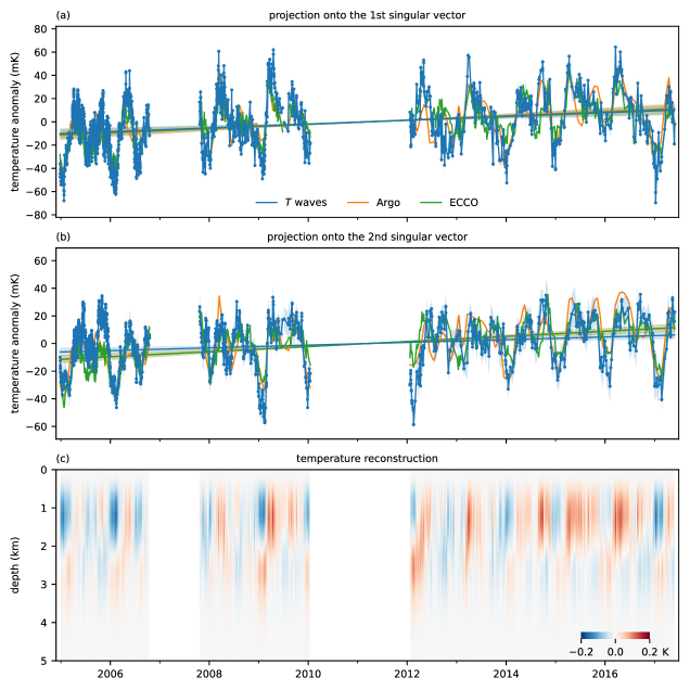
Figure 3: Inferred temperature anomalies for the path to Diego Garcia. Shown are (a), (b) the projections onto the first two singular vectors $\tilde{\boldsymbol{c}}_{2}$ for the T-wave data and two reference products and (c) the SVD reconstruction of the range-averaged temperature anomaly profile $\tilde{\boldsymbol{T}}_{2}$ obtained from the T-wave data. Each dot in (a) and (b) corresponds to an estimate at an event time, and the shading indicates $\pm 2\sigma$ confidence intervals around these estimates. Also shown are the estimated decadal trends of the projection coefficients $\tilde{\boldsymbol{c}}_{2}$, including their $\pm 2\sigma$ uncertainties.

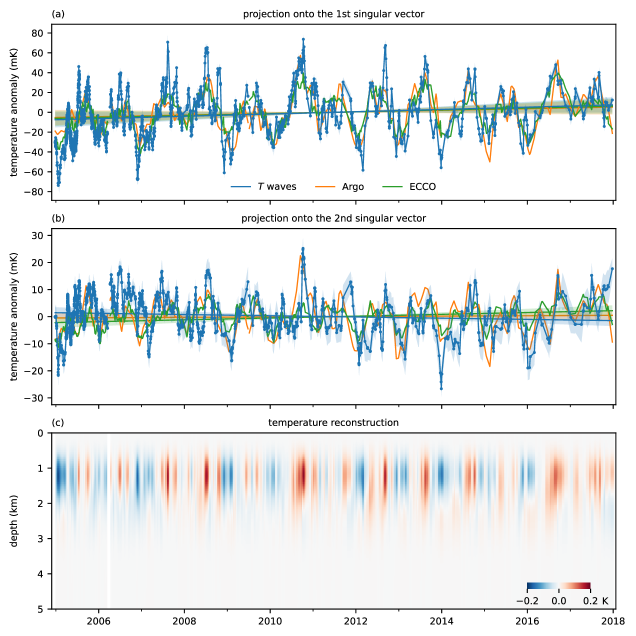
Figure 4: Inferred temperature anomalies for the path to Cape Leeuwin. Shown are (a), (b) the projections onto the first two singular vectors $\tilde{\boldsymbol{c}}_{2}$ for the T-wave data and two reference products and (c) the SVD reconstruction of the range-averaged temperature anomaly profile $\tilde{\boldsymbol{T}}_{2}$ obtained from the T-wave data. Each dot in (a) and (b) corresponds to an estimate at an event time, and the shading indicates $\pm 2\sigma$ confidence intervals around these estimates. Also shown are the estimated decadal trends of the projection coefficients $\tilde{\boldsymbol{c}}_{2}$, including their $\pm 2\sigma$ uncertainties.

		trends ($\mathrm{mK}\text{\,}{\mathrm{yr}}^{-1}$)		12 mo. ($\mathrm{mK}$)		6 mo. ($\mathrm{mK}$)
		1	2	1	2	1	2
Diego Garcia	T waves	$+1.6\pm 0.7$	$+1.1\pm 0.5$	$15\pm 4$	$12\pm 4$	$15\pm 4$	$11\pm 4$
	Argo	$+1.9\pm 0.7$	$+1.8\pm 0.5$	$\hphantom{0}9\pm 4$	$\hphantom{0}9\pm 1$	$12\pm 4$	$11\pm 2$
	ECCO	$+1.7\pm 0.7$	$+1.9\pm 0.5$	$\hphantom{0}8\pm 4$	$\hphantom{0}8\pm 2$	$11\pm 3$	$11\pm 3$
Cape Leeuwin	T waves	$+1.1\pm 1.2$	$-0.2\pm 0.3$	$20\pm 5$	$\hphantom{0}5\pm 5$	$\hphantom{0}3\pm 5$	$\hphantom{0}2\pm 5$
	Argo	$+0.8\pm 1.2$	$+0.1\pm 0.3$	$19\pm 5$	$\hphantom{0}5\pm 3$	$\hphantom{0}3\pm 4$	$\hphantom{0}3\pm 1$
	ECCO	$+1.0\pm 1.2$	$+0.3\pm 0.3$	$16\pm 5$	$\hphantom{0}3\pm 3$	$\hphantom{0}3\pm 4$	$\hphantom{0}3\pm 2$

Table 1: Trends and amplitudes of the annual and semi-annual signals inferred from T-wave data and previous products. These parameters are estimated for the temperature projections onto the first two singular vectors (columns labelled 1 and 2). All uncertainties are given as $\pm 2\sigma$.

Time series of the temperature profiles projected onto the first two singular vectors show prominent seasonal and sub-seasonal variations, as well as significant decadal trends for the path to Diego Garcia (Fig. 3a,b; 4a,b; Table 1). The first singular vectors have a similar shape as the kernels themselves, so their coefficients represent a weighted average of the deep temperature anomalies, with the weighting peaked at $1.5\text{~{}}\mathrm{km}1.3\text{~{}}\mathrm{km}$ for the paths to Diego Garcia and Cape Leeuwin, respectively (Fig. 2b,e). The second singular vectors have nodes at $1.7\text{~{}}\mathrm{km}1.5\text{~{}}\mathrm{km}$ for the two paths, so the projection onto them is more sensitive to where in the water column the anomalies are located.

These projections inferred from T-wave travel time anomalies show general agreement with previous products. We compare our estimates to monthly interpolated Argo data [29] and daily ECCO state estimate data [[, v4r4;]]Forget2015,ECCO2021. Using the sensitivity kernels, we infer travel time anomalies from the temperature anomalies of these products, interpolate those onto our event times, and subsequently treat them in the same way as the T-wave anomalies.

For the path to Diego Garcia, seasonal and sub-seasonal variations in both these projections tend to line up (Fig. 3a,b), indicating that the vertical structure inferred from the T-wave data is broadly consistent with these previous estimates. There are notable exceptions. The anomalies inferred from the T-wave data are stronger on average, particularly in the projection onto the first singular vector (Fig. 3a, Table 1). The projection onto the second singular vector (Fig. 3b) is more positive for the Argo product than for the T-wave data in the latter part of the time series, and it is less negative for ECCO than for the T-wave data in the early part of the time series, producing a stronger decadal trend in both previous products than inferred from the T-wave data (Table 1).

For the path to Cape Leeuwin, the seasonal variations in both projections are similar between those inferred from T-wave data and those from previous products (Fig. 4a,b). In contrast to the equatorial path to Diego Garcia, the annual signal here is much stronger than the semi-annual signal (Table 1). The T-wave data produces sizable spikes with a duration on the order of a month, which are typically missed by previous data (Fig. 4a,b; LABEL:fig:h01depth; LABEL:fig:h01invdepth). As discussed in W23, we interpret these spikes as resulting from mesoscale eddies traversing the path, most importantly those shed by the Leeuwin Current. The temperature anomalies of these eddies are largely confined to the thermocline [[, e.g.,]]Fieux2005, which is consistent with the anomalies in the two projections appearing in phase. At times, these eddies happen to be captured by Argo floats (e.g., 2005-10 and 2010-10), but they are more typically missed, as expected from the Argo float coverage (Fig. 1). ECCO does not capture mesoscale eddies because it has too low a horizontal resolution. The overall stronger variability along this path to Cape Leeuwin implies that decadal trends are more uncertain (Table 1), although the uncertainties in the estimation from the three data sources are not independent.

Time series of the temperature reconstruction $\tilde{\boldsymbol{T}}_{2}$ illustrate the information on the vertical structure contained in the T-wave data. On the path to Diego Garcia, the inferred temperature anomalies are strongest in the upper $2\text{~{}}\mathrm{km}$ but reach substantially below this depth (Fig. 3c). It cannot be inferred from the data whether these abyssal anomalies are real or whether they arise from the insufficient vertical resolution. (See Fig. LABEL:fig:h08depth, LABEL:fig:h01depth, LABEL:fig:h08invdepth, and LABEL:fig:h01invdepth for projections of Argo and ECCO data onto the first two singular vectors.) Nevertheless, the anomalies display an upward phase propagation that is expected for long surface-generated equatorial waves that have a downward energy flux [[, e.g.,]]Wunsch1977b,Philander1978,McPhaden1982,Luyten1982,Reppin1999. This upward phase propagation is not apparent on the extratropical path to Cape Leeuwin (Fig. 4c), where the inferred anomalies are more strongly confined to above $2\text{~{}}\mathrm{km}$ depth, consistent with mesoscale thermocline eddies.

In interpreting these results, it should be kept in mind that the sensitivity kernels are based on two-dimensional numerical simulations of the wave propagation from the source to the receiver [38]. These simulations depend, albeit not sensitively, on assumptions about the thickness and properties of sediment layers and on the neglect of off-geodesic effects. There is therefore representational uncertainty in our estimates of temperature anomalies and their vertical structure arising from uncertainty in the kernels. More work is needed to better understand these effects.

4 Conclusions

The data presented here demonstrate that changes in T-wave travel times contain information on the vertical structure of the temperature anomalies encountered by these waves along their paths. This information can be extracted from travel time anomalies at a few low frequencies even though the sensitivity kernels at these frequencies have similar vertical structures (Fig. 2).

We here illustrated this vertical structure using a simple SVD inversion. In the future, the T-wave data should be combined with Argo and ship-based hydrographic data, either using a relatively simple mapping as typically employed for Argo data or using state estimation as in ECCO, which also allows one to incorporate additional constraints, for example from altimetry and gravitometry. T waves offer constraints on the large-scale temperature changes that are complementary to previous data. They intrinsically average in space, so they do not miss mesoscale eddies like the Argo array. They offer a dense sampling in time, which is important even for large-scale averages that still contain sizable anomalies induced by equatorial waves and mesoscale eddies. T waves offer constraints on the ocean below $2\text{~{}}\mathrm{km}$ depth, which has been sparsely sampled in space and time by ship-based hydrographic surveys. The vertical resolution obtained from T-wave is relatively coarse, but they nevertheless constrain the vertical structure of the large-scale temperature anomalies.

In the present work, we restricted ourselves to low frequencies because the waveform correlation drops substantially at higher frequencies (Fig. 1b) and travel time changes cannot be extracted confidently. The T-wave signals have plenty of power at these higher frequencies, so noise is unlikely to be the problem. Instead, we speculate that the higher-frequency signals contain multiple vertical acoustic modes. The modes become more confined in the vertical as the frequency increases, so more modes escape interaction with the bottom and subsequent attenuation. Different modes experience different time shifts, so the waveform correlation drops if multiple modes contribute substantially. If this interpretation is correct, much more detailed information on the vertical structure could be extracted if we were able to separate the modes in the received signal, for example using a vertical hydrophone array [4]. Deploying such arrays is routine, so future T-wave measurements could yield much stronger constraints on the vertical structure of the ocean’s large-scale temperature variability.

Open research

The IMS hydrophone data are available directly from the CTBTO upon request and signing a confidentiality agreement to access the virtual Data Exploitation Centre (vDEC). All seismic data were downloaded through the IRIS Data Management Center (https://service.iris.edu/), including the seismic networks II (GSN; https://doi.org/10.7914/SN/II), MY, PS, and GE (https://doi.org/10.14470/TR560404). The Global Seismographic Network (GSN) is a cooperative scientific facility operated jointly by the Incorporated Research Institutions for Seismology (IRIS), the United States Geological Survey (USGS) and the National Science Foundation (NSF), under Cooperative Agreement EAR-1261681. The processing code is available at https://github.com/joernc/SOT.

Disclaimer

The views expressed in the paper are those of the authors and do not necessarily represent those of the CTBTO.

References

- [1] Bruce D. Cornuelle, Peter F. Worcester, John A. Hildebrand, William S. Hodgkiss Jr., Timothy F. Duda, Janice Boyd, Bruce M. Howe, James A. Mercer and Robert C. Spindel “Ocean Acoustic Tomography at 1000-Km Range Using Wavefronts Measured with a Large-Aperture Vertical Array” In Journal of Geophysical Research: Oceans 98.C9, 1993, pp. 16365–16377 DOI: 10.1029/93JC01246
- [2] Damien Desbruyères, Elaine L. McDonagh, Brian A. King and Virginie Thierry “Global and Full-Depth Ocean Temperature Trends during the Early Twenty-First Century from Argo and Repeat Hydrography” In Journal of Climate 30, 2017, pp. 1985–1997 DOI: 10.1175/JCLI-D-16-0396.1
- [3] Damien G. Desbruyères, Sarah G. Purkey, Elaine L. McDonagh, Gregory C. Johnson and Brian A. King “Deep and abyssal ocean warming from 35 years of repeat hydrography” In Geophysical Research Letters 43, 2016, pp. 10,356–10,365 DOI: 10.1002/2016GL070413
- [4] Gerald L. D’Spain, Lewis P. Berger, W. A. Kuperman, Jeffry L. Stevens and G. Eli Baker “Normal mode composition of earthquake T phases” In Monitoring the Comprehensive Nuclear-Test-Ban Treaty: Hydroacoustics 158 Birkhäuser, 2001, pp. 475–512 DOI: 10.1007/978-3-0348-8270-5_4
- [5] B. D. Dushaw et al. “A decade of acoustic thermometry in the North Pacific Ocean” In Journal of Geophysical Research: Oceans 114, 2009, pp. 1–24 DOI: 10.1029/2008JC005124
- [6] Brian D. Dushaw “Inversion of multimegameter-range acoustic data for ocean temperature” In IEEE Journal of Oceanic Engineering 24, 1999, pp. 215–223 DOI: 10.1109/48.757272
- [7] Brian D. Dushaw “Ocean acoustic tomography in the North Atlantic” In Journal of Atmospheric and Oceanic Technology 36, 2019, pp. 183–202 DOI: 10.1175/JTECH-D-18-0082.1
- [8] ECCO Consortium “Synopsis of the ECCO Central Production Global Ocean and Sea-Ice State Estimate”, 2021, pp. 17 DOI: 10.5281/zenodo.4533349
- [9] Michèle Fieux, Robert Molcard and Rosemary Morrow “Water properties and transport of the Leeuwin Current and Eddies off Western Australia” In Deep-Sea Research Part I: Oceanographic Research Papers 52, 2005, pp. 1617–1635 DOI: 10.1016/j.dsr.2005.03.013
- [10] G. Forget, J. M. Campin, P. Heimbach, C. N. Hill, R. M. Ponte and C. Wunsch “ECCO version 4: An integrated framework for non-linear inverse modeling and global ocean state estimation” In Geoscientific Model Development 8, 2015, pp. 3071–3104 DOI: 10.5194/gmd-8-3071-2015
- [11] Qiang Fu, Celeste M. Johanson, Stephen G. Warren and Dian J. Seidel “Contribution of stratospheric cooling to satellite-inferred tropospheric temperature trends” In Nature 429, 2004, pp. 55–58 DOI: 10.1038/nature02524
- [12] J. M. Gregory “Vertical heat transports in the ocean and their effect on time-dependent climate change” In Climate Dynamics 16, 2000, pp. 501–515 DOI: 10.1007/s003820000059
- [13] J. Hansen, A. Lacis, D. Rind, G. Russell, P. Stone, I. Fung, R. Ruedy and J. Lerner “Climate Sensitivity: Analysis of Feedback Mechanisms” In Climate Processes and Climate Sensitivity 29, 1981, pp. 337–351 DOI: 10.1029/GM029p0130
- [14] Isaac M. Held, Michael Winton, Ken Takahashi, Thomas Delworth, Fanrong Zeng and Geoffrey K. Vallis “Probing the fast and slow components of global warming by returning abruptly to preindustrial forcing” In Journal of Climate 23, 2010, pp. 2418–2427 DOI: 10.1175/2009JCLI3466.1
- [15] Gregory C. Johnson, Chanelle Cadot, John M. Lyman, Kristene E. McTaggart and Elizabeth L. Steffen “Antarctic Bottom Water Warming in the Brazil Basin: 1990s Through 2020, From WOCE to Deep Argo” In Geophysical Research Letters 47, 2020 DOI: 10.1029/2020GL089191
- [16] Yavor Kostov, Kyle C. Armour and John Marshall “Impact of the Atlantic meridional overturning circulation on ocean heat storage and transient climate change” In Geophysical Research Letters 41, 2014, pp. 2108–2116 DOI: 10.1002/2013GL058998
- [17] James R. Luyten and Dean H. Roemmich “Equatorial Currents at Semi-Annual Period in the Indian Ocean” In Journal of Physical Oceanography 12, 1982, pp. 406–413 DOI: 10.1175/1520-0485(1982)012<0406:ECASAP>2.0.CO;2
- [18] M J McPhaden “Variability in the central equatorial Indian Ocean. Part I: Ocean dynamics” In Journal of Marine Research 40, 1982, pp. 157–176
- [19] W. H. Munk and A. M. G. Forbes “Global Ocean Warming: An Acoustic Measure?” In Journal of Physical Oceanography 19, 1989, pp. 1765–1778 DOI: 10.1175/1520-0485(1989)019<1765:gowaam>2.0.co;2
- [20] Walter Munk, Peter Worcester and Carl Wunsch “Ocean Acoustic Tomography” Cambridge University Press, 1995, pp. 433
- [21] Walter Munk and Carl Wunsch “Ocean acoustic tomography: a scheme for large scale monitoring” In Deep Sea Research Part A, Oceanographic Research Papers 26, 1979, pp. 123–161 DOI: 10.1016/0198-0149(79)90073-6
- [22] Walter Munk and Carl Wunsch “Up–down resolution in ocean acoustic tomography” In Deep Sea Research Part A, Oceanographic Research Papers 29, 1982, pp. 1415–1436 DOI: 10.1016/0198-0149(82)90034-6
- [23] Walter Munk and Carl Wunsch “Ocean acoustic tomography: Rays and modes” In Reviews of Geophysics and Space Physics 21, 1983, pp. 777–793 DOI: 10.1029/RG021i004p00777
- [24] Emile A. Okal “The generation of T waves by earthquakes” In Advances in Geophysics 49 Elsevier, 2008, pp. 1–65 DOI: 10.1016/S0065-2687(07)49001-X
- [25] S. G.H. Philander “Forced oceanic waves” In Reviews of Geophysics 16, 1978, pp. 15–46 DOI: 10.1029/RG016i001p00015
- [26] Sarah G. Purkey and Gregory C. Johnson “Warming of Global Abyssal and Deep Southern Ocean Waters between the 1990s and 2000s: Contributions to Global Heat and Sea Level Rise Budgets” In Journal of Climate 23, 2010, pp. 6336–6351 DOI: 10.1175/2010JCLI3682.1
- [27] Jörg Reppin, Friedrich A. Schott, Jürgen Fischer and Detlef Quadfasel “Equatorial currents and transports in the upper central Indian Ocean: Annual cycle and interannual variability” In Journal of Geophysical Research: Oceans 104, 1999, pp. 15495–15514 DOI: 10.1029/1999jc900093
- [28] Dean Roemmich, John Church, John Gilson, Didier Monselesan, Philip Sutton and Susan Wijffels “Unabated planetary warming and its ocean structure since 2006” In Nature Climate Change 5, 2015, pp. 240–245 DOI: 10.1038/nclimate2513
- [29] Dean Roemmich and John Gilson “The 2004–2008 mean and annual cycle of temperature, salinity, and steric height in the global ocean from the Argo Program” In Progress in Oceanography 82 Elsevier Ltd, 2009, pp. 81–100 DOI: 10.1016/j.pocean.2009.03.004
- [30] Dean Roemmich and Carl Wunsch “Apparent changes in the climatic state of the deep North Atlantic Ocean” In Nature 307, 1984, pp. 447–450 DOI: 10.1038/307447a0
- [31] Dean Roemmich et al. “On the future of Argo: A global, full-depth, multi-disciplinary array” In Frontiers in Marine Science 6, 2019, pp. 439 DOI: 10.3389/fmars.2019.00439
- [32] E. C. Shang “Ocean Acoustic Tomography Based On Adiabatic Mode Theory” In Journal of the Acoustical Society of America 85, 1989, pp. 1531–1537 DOI: 10.1121/1.397355
- [33] John L. Spiesberger, Robert C Spindel and Kurt Metzger “Stability and identification of ocean acoustic multipaths” In Journal of the Acoustical Society of America 67, 1980, pp. 2011–2017 DOI: 10.1121/1.384441
- [34] The ATOC Consortium “Ocean Climate Change: Comparison of Acoustic Tomography, Satellite Altimetry, and Modeling” In Science 281, 1998, pp. 1327–1332 DOI: 10.1126/science.281.5381.1327
- [35] The Ocean Tomography Group “A demonstration of ocean acoustic tomography” In Nature 299, 1982, pp. 121–125 DOI: 10.1038/299121a0
- [36] Denis L. Volkov, Sang Ki Lee, Felix W. Landerer and Rick Lumpkin “Decade-long deep-ocean warming detected in the subtropical South Pacific” In Geophysical Research Letters 44, 2017, pp. 927–936 DOI: 10.1002/2016GL071661
- [37] Peter F. Worcester et al. “A test of basin-scale acoustic thermometry using a large-aperture vertical array at 3250-km range in the eastern North Pacific Ocean” In The Journal of the Acoustical Society of America 105, 1999, pp. 3185–3201 DOI: 10.1121/1.424649
- [38] Wenbo Wu, Zhongwen Zhan, Shirui Peng, Sidao Ni and Jörn Callies “Seismic ocean thermometry” In Science 1515, 2020, pp. 1510–1515 DOI: 10.1126/science.abb9519
- [39] Carl Wunsch “Response of an Equatorial Ocean to Periodic Monsoon” In Journal of Physical Oceanography 7, 1977, pp. 497–511 DOI: 10.1175/1520-0485(1977)007<0497:ROAEOT>2.0.CO;2
- [40] Carl Wunsch “Global Ocean Integrals and Means, with Trend Implications” In Annual Review of Marine Science 8, 2016, pp. 1–33 DOI: 10.1146/annurev-marine-122414-034040
- [41] Carl Wunsch and Patrick Heimbach “Practical global oceanic state estimation” In Physica D: Nonlinear Phenomena 230, 2007, pp. 197–208 DOI: 10.1016/j.physd.2006.09.040
- [42] Carl Wunsch and Patrick Heimbach “Bidecadal Thermal Changes in the Abyssal Ocean” In Journal of Physical Oceanography 44, 2014, pp. 2013–2030 DOI: 10.1175/JPO-D-13-096.1