The Colorado Ultraviolet Transit Experiment (CUTE) signal to noise calculator

Abstract

We present here the signal-to-noise (S/N) calculator developed for the Colorado Ultraviolet Transit Experiment (CUTE) mission. CUTE is a 6U CubeSat operating in the near-ultraviolet (NUV) observing exoplanetary transits to study their upper atmospheres. CUTE was launched into a low-Earth orbit in September 2021 and it is currently gathering scientific data. As part of the S/N calculator, we also present the error propagation for computing transit depth uncertainties starting from the S/N of the original spectroscopic observations. The CUTE S/N calculator is currently extensively used for target selection and scheduling. The modular construction of the CUTE S/N calculator enables its adaptation and can be used also for other missions and instruments.

1 Introduction

The detection of the first exoplanets has opened a new field in astrophysics (Mayor and Queloz, 1995; Charbonneau et al, 2000) and the finding that numerous exoplanets orbit close to their host stars has fostered studies of planet atmospheric mass loss (e.g. Vidal-Madjar et al, 2003; Lammer et al, 2003). These have then led to the conclusion that atmospheric escape plays a pivotal role in the long-term evolution of planetary atmospheres and in sculpting the observed exoplanet population (e.g. Jin et al, 2014; Jin and Mordasini, 2018; Owen and Lai, 2018; Kubyshkina et al, 2020).

The majority of the observational studies of exoplanet atmospheric escape have been performed at ultraviolet (UV) wavelengths by the Hubble Space Telescope (HST). These have led to the detection of both hydrogen and metals (Mg, Fe etc.) in the upper atmospheres, beyond the planetary Roche lobe, for a number of close-in planets (e.g. Vidal-Madjar et al, 2004; Fossati et al, 2010; Ehrenreich et al, 2015; Sing et al, 2019; Cubillos et al, 2020; García Muñoz et al, 2021). These observations have demonstrated that the upper atmospheres of close-in giant planets are hydrodynamically escaping as a result of the absorption, and consequent atmospheric heating, of the stellar high-energy (X-ray and extreme ultraviolet) emission (e.g. Yelle, 2004; García Muñoz, 2007; Koskinen et al, 2014). More recently, the Hei metastable near infrared triplet at $\approx$10830 Å, which is observable from the ground, has become an important tracer of atmospheric escape, but the strong dependence of the presence and strength of planetary Hei absorption on stellar type and He abundance (Oklopčić, 2019; Fossati et al, 2022) leaves UV transmission spectroscopy as the main workhorse to study atmospheric mass loss.

HST is the only facility currently available for studying exoplanetary upper atmospheres and escape at UV wavelengths. However, the shared-use nature of HST limits the number of planets that can be observed and, more importantly, the number of transits that can be observed for each planet, preventing for example to study transit variability in association with stellar variability due to activity. The Colorado Ultraviolet Transit Experiment is a 6U CubeSat mission fully dedicated to observe exoplanetary transits at near-UV wavelengths to study upper atmospheres and escape (Fleming et al, 2018; France et al, 2023; Egan et al, 2023; Sreejith et al, 2022).

We present here the CUTE signal-to-noise (S/N) calculator, which is available both as a website or as standalone downloadable software. This tool is extensively being used by the CUTE science and instrument teams to guide target selection. In Section 2, we present the implementation of the S/N calculator. In Section 3, we describe the web interface and its development, while the summary and the conclusions are presented in Section 4.

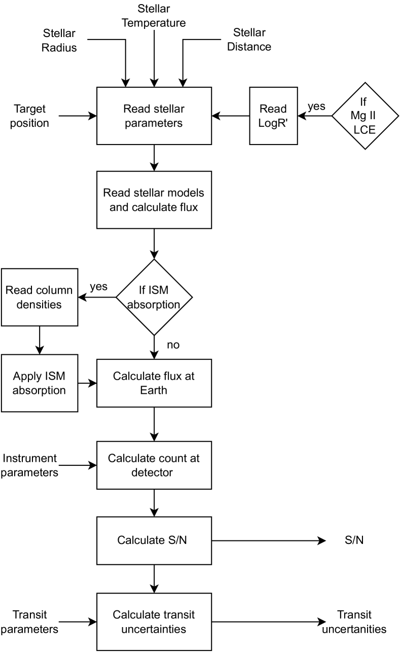
Figure 1: Flowchart of the CUTE S/N calculator. In the top-right, LCE stands for “line core emission”.

2 Implementation

2.1 General structure

The CUTE S/N calculator is an offshoot of the CUTE data simulator (Sreejith et al, 2019), which takes stellar models, stellar parameters, instrument specifications, and planetary transit information as input to generate simulated CUTE data that can be used to simulate transit lightcurves in the CUTE band, including their uncertainties. Figure 1 presents the overall working flowchart of the CUTE S/N calculator. The code reads the input parameters to generate a spectrum of the target star in the CUTE band by employing a library of synthetic photospheric stellar fluxes. The available library of stellar flux models has been generated employing the LLmodels stellar atmosphere code (Shulyak et al, 2004), which computes photospheric fluxes of stars assuming local thermodynamical equilibrium (LTE). This library covers stars raging between 3500 K and 12000 K, in steps of 100 K below 6800 K and in steps of 200 K above it, with a wavelength sampling of 0.005 Å between 1500 and 9000 Å.

The CUTE spectrograph also covers the Mgii h&k resonance lines, which in late-type stars present chromospheric line core emission (LCE) with a strength proportional to the stellar activity. The code automatically estimates the Mgii h&k line core emission from the $\log R^{\prime}_{\rm HK}$ value and the stellar radius given in input (Fossati et al, 2017; Sreejith et al, 2020). The stellar flux at Earth is then derived by scaling for the distance to the star calculated from the parallax provided by the user.

The CUTE S/N calculator also accounts for interstellar medium (ISM) absorption. In particular, we implemented both broadband extinction and ISM line absorption for Mg and Fe at the position of the NUV Mgi (2852.127 Å), Mgii (2795.528 Å and 2802.705 Å), and Feii (2599.395 Å) resonance lines (Sreejith et al, 2019). Each ISM absorption feature is simulated as a single Voigt profile with a $b$-parameter (i.e. broadening) of 3 km s^-1 (Malamut et al, 2014) and assuming for no radial velocity shift between the stellar and ISM features as radial velocity shift has an negligible impact on transit measurements at the CUTE resolution (Sreejith et al, 2023). The Mgi, Mgii, and Feii ISM column densities ($\log N_{\rm ion}$), which set the strength of the ISM absorption features, are required input from the user, who can use the algorthm described by (Sreejith et al, 2019) to estimate the ISM column densities for each individual species.

The stellar flux at Earth, optionally modified to account for the ISM absorption, is then converted from erg cm^-2 s^-1 Å^-1 to photons cm^-2 s^-1 Å^-1. The spectra are then trimmed to the relevant wavelength range (2478–3305 Å in the case of CUTE), multiplied by the effective area of the instrument, and convolved to the spectrograph’s resolution, finally obtaining the CCD detector counts (counts Å^-1 s^-1). As a further step, the S/N calculator converts the counts Å^-1 s^-1 to counts pixel^-1 s^-1 by taking into account the spectral resolution and the number of pixels per resolution element. Finally, the CCD counts are multiplied by the exposure time to obtain the expected signal from a particular source. The CCD counts are further converted from counts to photo-electrons using the gain provided by the user. The noise calculation is described in Section 2.3, while here below we detail the input parameters requested by the code.

2.2 Input Parameters

2.2.1 Stellar Parameters

Temperature: Temperature of the star in Kelvin. The stellar model to employ is selected on the basis of the given temperature and it sets the shape of the stellar spectral energy distribution (SED).

Radius: Radius of the star in solar radii.

Coordinates: Right ascension and declination of the star in degrees in J2000. This information is used to calculate the extinction and ISM column densities.

Distance: Distance to the star as parallax in milliarcseconds (mas). This is used to scale the stellar SED at Earth.

Stellar activity index: Stellar activity index ($\log R^{\prime}_{\mathrm{HK}}$) of the star. This parameter is used to set the strength of the Mgii h&k line core emission.

Line core emission: If this option is enabled, it adds the line core emission at the position of Mgii h&k resonance lines assuming that the behaviour of the Mgii h&k emission with stellar temperature is comparable to that of the Caii H&K emission.

Interstellar medium absorption: The S/N calculator adds extinction following the method described in Sreejith et al (2019). The user has the option to add ISM absorption at the position of any of the three Mg and Fe main resonance lines in the CUTE band: Mgi (2852.127 Å), Mgii (2795.528 Å and 2802.705 Å), and Feii (2599.395 Å). If ISM absorption is enabled, the user has to provide the column densities of the corresponding species and to estimate them users can either use the method described in Sreejith et al (2019) or employ the calc_cd code available with the CUTE S/N software distribution.

2.2.2 Instrumental Parameters

Spectral Resolution: Spectral resolution of the spectrograph in angstroms.

CCD readout noise: The CCD readout noise in electrons pixel^-1.

CCD dark noise: The CCD dark noise in electrons pixel^-1 s^-1.

CCD gain: The CCD gain in photoelectrons ADU^-1.

Spectrum width: Expected width in the cross-dispersion direction of the spectrum in pixels.

Exposure time: Exposure time for each observation in seconds.

CCD read time: The CCD read time for each observation in seconds.

In addition to these parameters, the calculator requires the effective area of the instrument and the wavelength to pixel solution. In the case of CUTE, these profiles are available with the software distribution and are those used also by the web interface.

2.2.3 Transit Parameters

The exoplanetary transit parameters required by the S/N calculator are the transit duration of the planet in hours and the total number of transit observations.

2.2.4 Wavelength Parameters

By default the S/N calculator computes the noise level in seven bands, as described in table 1. In addition to these bands, the user can specify a maximum of 20 wavelength bands of specific interest.

Table 1: Wavelength bands for CUTE S/N calculator.

Band	Range (in Å)
Full Band	2478.48–3304.86
Lower Band	2478.48–2788.84
Mid Band	2789.24–3059.57
Upper Band	3059.97–3304.86
Mgii Band	2792.81–2804.72
Mgi Band	2849.97–2853.54
Feii Band	2582.81–2586.78

2.3 Noise Propagation

The S/N calculator considers three main sources of noise.

Read noise of the CCD detector. In most of the modern cooled scientific CCDs, the readout noise sets a limit on the detector’s performance and can be reduced at the expense of increasing readout time.

Dark noise in the detector due to thermal CCD electrons. Dark noise is reduced by operating the CCD at low temperatures inhibiting the creation of thermal electrons.

Photon noise that is assumed to follow a Poissonian distribution, and thus computed as the square root of the number of incoming photons.

Considering these noise components the $S/N$ ratio of the stellar spectrum extracted from the CCD, $\frac{S}{N}\big{|}_{F}$ is

$$\frac{S}{N}\Big{|}_{F}=\frac{F}{\sigma_{F}}.$$ (1)

where $F$ is the integrated CCD counts in photo-electrons in the wavelength range of interest and $\sigma_{F}$ is the related uncertainty. In particular,

$$F=\sum{\Delta\lambda F_{\lambda}}$$ (2)

and

$$\sigma_{F}^{2}=\sum{(\Delta\lambda\,\,\sigma_{F_{\lambda}})^{2}}\,,$$ (3)

where $\Delta\lambda$ is the considered wavelength range, $F_{\lambda}$ is the expected counts value (in photo-electrons) as a function of wavelength and $\sigma_{F_{\lambda}}$ is the respective uncertainty that is computed as

$$\sigma_{F_{\lambda}}=\sqrt{{\rm p\_noise_{\lambda}}^{2}+{\rm s\_width}\,({\rm r\_noise}^{2}+({\rm d\_noise_{\lambda}}\times{\rm exptime}\times G))}\,.$$ (4)

In Equation (4), p_noise_λ is the photon noise associated with the signal at each wavelength ${\lambda}$, r_noise is the read noise of the CCD in ADU, d_noise_λ is the dark noise of the CCD in electron s^-1 pixel^-1, exptime is the exposure time of the observation, $G$ is the CCD gain, and s_width specifies the cross-dispersion width of the spectrum in pixels. All these parameters are user inputs except for the photon noise which is calculated as $\sqrt{F_{\lambda}}$.

2.4 Transit uncertainties

The S/N calculator then combines the available information to compute the final uncertainty on the transit depth, which the instrument is expected to be capable to measure following one transit observation or by combining multiple transits, as follows. The S/N ratio of the transit depth measurement is

$$\frac{S}{N}\Bigg{|}_{d}=\frac{d}{\sigma_{d}}\,,$$ (5)

where $d$ is the transit depth and $\sigma_{d}$ its uncertainty. The former can be written as

$$d=1-\frac{F_{\rm in}}{F_{\rm out}}=\left(\frac{R_{\rm p}}{R_{\rm s}}\right)^{2}\,,$$ (6)

where $F_{\rm in}$ is the in-transit flux, $F_{\rm out}$ is the out of transit flux, $R_{\rm p}$ is the planetary radius, and $R_{\rm s}$ is the stellar radius. Therefore, the uncertainty on the transit depth, ignoring the uncertainty on the stellar radius, can be written as

$$\sigma_{d}=\frac{\partial d}{\partial R_{\rm p}}\sigma_{R_{\rm p}}=\frac{2R_{\rm p}}{R_{\rm s}^{2}}\sigma_{R_{\rm p}}=\frac{2d}{R_{\rm p}}\sigma_{R_{\rm p}}\,,$$ (7)

where $\sigma_{R_{\rm p}}$ is the uncertainty on the planetary radius, which then becomes

$$\sigma_{R_{\rm p}}=\frac{R_{\rm p}}{2d}\sigma_{d}=\frac{R_{\rm p}}{2\frac{S}{N}\big{|}_{d}}\,.$$ (8)

By combining Equation (6) and Equation (1), one obtains

$$\sigma_{d} =\sqrt{\left(\frac{\partial d}{\partial F_{\rm out}}\right)^{2}\sigma_{F_{\rm out}}^{2}+\left(\frac{\partial d}{\partial F_{\rm in}}\right)^{2}\sigma_{F_{\rm in}}^{2}}$$

$$=\sqrt{\left(\frac{F_{\rm in}}{F_{\rm out}^{2}}\right)^{2}\sigma_{F_{\rm out}}^{2}+\left(\frac{1}{F_{\rm out}}\right)^{2}\sigma_{F_{\rm in}}^{2}}\,,$$ (9)

where $\sigma_{F_{\rm in}}$ and $\sigma_{F_{\rm out}}$ are the uncertainties on the in- and out of transit fluxes, respectively. Then, assuming $F_{\rm in}$ $\approx$ $F_{\rm out}$ $\equiv$ $F$ and $\sigma_{F_{\rm in}}$ $\approx$ $\sigma_{F_{\rm out}}$ $\equiv$ $\sigma_{F}$, one obtains

$$\sigma_{d}=\sqrt{\left(\frac{F}{F^{2}}\right)^{2}\sigma_{F}^{2}+\left(\frac{1}{F}\right)^{2}\sigma_{F}^{2}}=\sqrt{2\left(\frac{1}{F}\right)^{2}\sigma_{F}^{2}}=\sqrt{2}\frac{\sigma_{F}}{F}=\frac{\sqrt{2}}{\frac{S}{N}\big{|}_{F}}\,.$$ (10)

Therefore,

$$\frac{S}{N}\Big{|}_{d}=\frac{d}{\sqrt{2}\frac{\sigma_{F}}{F}}=\frac{d}{\sqrt{2}}\frac{S}{N}\Big{|}_{F}\,,$$ (11)

which implies that the uncertainty on the planetary radius as a function of the S/N of the observed spectra is

$$\sigma_{R_{\rm p}}=\frac{R_{\rm p}}{2\frac{d}{\sqrt{2}}\frac{S}{N}\big{|}_{F}}\,.$$ (12)

3 Web Interface

The web application of the CUTE S/N calculator has been developed on Python Flask web framework, which makes use of the Jinja template engine and the Werkzeug (WSGI) toolkit. Figure 2 shows the main web page of the S/N calculator. The web application accepts input values from the user, validates the inputs, and run the S/N calculator, finally providing the user with the results. The validation of the input values is carried out by the server and users are notified in case of problems. The server reads the user input form and generates the necessary parameters for the S/N calculations.

The output web page, shown in Figure 3, displays an example result of a S/N calculation, which contains also a quick look image that we show in Figure 4. The basic output given on the web page is that of the S/N ratio and relative uncertainties on the transit depth as a function of wavelength. Furthermore, the S/N calculator enables the user to download a file detailing all outputs of the simulation for further analysis.

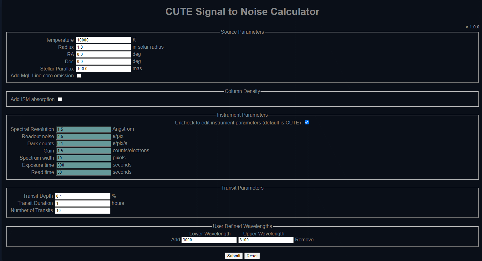
Figure 2: Input web page of the CUTE S/N calculator.

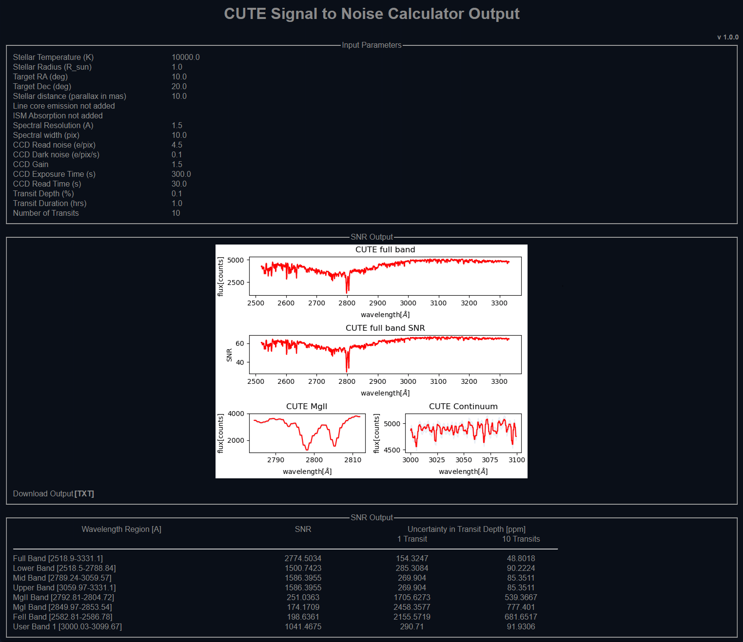
Figure 3: Example output web page of the CUTE S/N calculator.

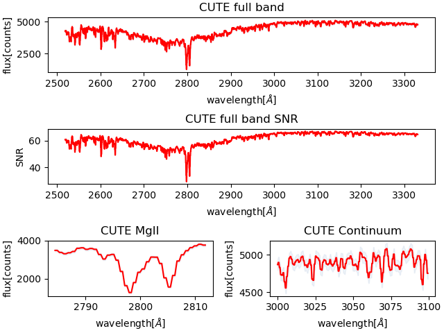
Figure 4: Blow up of the plot shown in Figure 3.

4 Summary and Conclusion

We presented the CUTE S/N calculator and its implementation as a web form. The modular approach of the calculator enables one to easily modify it to the needs of future missions and instruments carrying out transmission spectroscopy. The development of a web version also enables one to use the calculator without the need to install extra software or computational resources.

In the future, we plan to introduce additional features that would make the S/N calculator more general and easy to use, the most important being

• Option to upload a stellar model file;

• Option to upload both effective area and wavelength solution files;

• Option to consider ISM absorption at other wavelengths;

• Option to derive stellar parameters from the target name, for example through querying the latest GAIA catalog.

• Evaluating the effect of different scatter light on S/N calculations.

References

- \bibcommenthead
- Charbonneau et al (2000) Charbonneau D, Brown TM, Latham DW, et al (2000) Detection of Planetary Transits Across a Sun-like Star. The Astrophysical Journal Letter 529(1):L45–L48. 10.1086/312457, https://arxiv.org/abs/arXiv:astro-ph/9911436 [astro-ph]
- Cubillos et al (2020) Cubillos PE, Fossati L, Koskinen T, et al (2020) Near-ultraviolet Transmission Spectroscopy of HD 209458b: Evidence of Ionized Iron Beyond the Planetary Roche Lobe. The Astronomical Journal 159(3):111. 10.3847/1538-3881/ab6a0b, https://arxiv.org/abs/arXiv:2001.03126 [astro-ph.EP]
- Egan et al (2023) Egan A, Nell N, Suresh A, et al (2023) The On-orbit Performance of the Colorado Ultraviolet Transit Experiment Mission. The Astronomical Journal 165(2):64. 10.3847/1538-3881/aca8a3, https://arxiv.org/abs/arXiv:2301.01307 [astro-ph.IM]
- Ehrenreich et al (2015) Ehrenreich D, Bourrier V, Wheatley PJ, et al (2015) A giant comet-like cloud of hydrogen escaping the warm Neptune-mass exoplanet GJ 436b. Nature 522(7557):459–461. 10.1038/nature14501, https://arxiv.org/abs/arXiv:1506.07541 [astro-ph.EP]
- Fleming et al (2018) Fleming BT, France K, Nell N, et al (2018) Colorado Ultraviolet Transit Experiment: a dedicated CubeSat mission to study exoplanetary mass loss and magnetic fields. Journal of Astronomical Telescopes, Instruments, and Systems 4:014004. 10.1117/1.JATIS.4.1.014004, https://arxiv.org/abs/arXiv:1801.02673 [astro-ph.IM]
- Fossati et al (2010) Fossati L, Haswell CA, Froning CS, et al (2010) Metals in the Exosphere of the Highly Irradiated Planet WASP-12b. The Astrophysical Journal Letter 714(2):L222–L227. 10.1088/2041-8205/714/2/L222, https://arxiv.org/abs/arXiv:1005.3656 [astro-ph.SR]
- Fossati et al (2017) Fossati L, Erkaev NV, Lammer H, et al (2017) Aeronomical constraints to the minimum mass and maximum radius of hot low-mass planets. Astronomy and Astrophysics 598:A90. 10.1051/0004-6361/201629716, https://arxiv.org/abs/arXiv:1612.05624 [astro-ph.EP]
- Fossati et al (2022) Fossati L, Guilluy G, Shaikhislamov IF, et al (2022) The GAPS Programme at TNG. XXXII. The revealing non-detection of metastable He I in the atmosphere of the hot Jupiter WASP-80b. Astronomy and Astrophysics 658:A136. 10.1051/0004-6361/202142336, https://arxiv.org/abs/arXiv:2112.11179 [astro-ph.EP]
- France et al (2023) France K, Fleming B, Egan A, et al (2023) The Colorado Ultraviolet Transit Experiment Mission Overview. The Astronomical Journal 165(2):63. 10.3847/1538-3881/aca8a2, https://arxiv.org/abs/arXiv:2301.02250 [astro-ph.IM]
- García Muñoz (2007) García Muñoz A (2007) Physical and chemical aeronomy of HD 209458b. Planetary and Space Science 55(10):1426–1455. 10.1016/j.pss.2007.03.007
- García Muñoz et al (2021) García Muñoz A, Fossati L, Youngblood A, et al (2021) A Heavy Molecular Weight Atmosphere for the Super-Earth Men c. The Astrophysical Journal Letters 907(2):L36. 10.3847/2041-8213/abd9b8, https://arxiv.org/abs/arXiv:2102.00203 [astro-ph.EP]
- Jin and Mordasini (2018) Jin S, Mordasini C (2018) Compositional Imprints in Density-Distance-Time: A Rocky Composition for Close-in Low-mass Exoplanets from the Location of the Valley of Evaporation. The Astrophysical Journal 853(2):163. 10.3847/1538-4357/aa9f1e, https://arxiv.org/abs/arXiv:1706.00251 [astro-ph.EP]
- Jin et al (2014) Jin S, Mordasini C, Parmentier V, et al (2014) Planetary Population Synthesis Coupled with Atmospheric Escape: A Statistical View of Evaporation. The Astrophysical Journal 795(1):65. 10.1088/0004-637X/795/1/65, https://arxiv.org/abs/arXiv:1409.2879 [astro-ph.EP]
- Koskinen et al (2014) Koskinen TT, Lavvas P, Harris MJ, et al (2014) Thermal escape from extrasolar giant planets. Philosophical Transactions of the Royal Society of London Series A 372(2014):20130,089–20130,089. 10.1098/rsta.2013.0089, https://arxiv.org/abs/arXiv:1312.1947 [astro-ph.EP]
- Kubyshkina et al (2020) Kubyshkina D, Vidotto AA, Fossati L, et al (2020) Coupling thermal evolution of planets and hydrodynamic atmospheric escape in MESA. Monthly Notices of the Royal Astronomical Society 499(1):77–88. 10.1093/mnras/staa2815, https://arxiv.org/abs/arXiv:2009.04948 [astro-ph.EP]
- Lammer et al (2003) Lammer H, Selsis F, Ribas I, et al (2003) Atmospheric Loss of Exoplanets Resulting from Stellar X-Ray and Extreme-Ultraviolet Heating. The Astrophysical Journal Letter 598(2):L121–L124. 10.1086/380815
- Malamut et al (2014) Malamut C, Redfield S, Linsky JL, et al (2014) The Structure of the Local Interstellar Medium. VI. New Mg II, Fe II, and Mn II Observations toward Stars within 100 pc. The Astrophysical Journal 787(1):75. 10.1088/0004-637X/787/1/75, https://arxiv.org/abs/arXiv:1403.8096 [astro-ph.SR]
- Mayor and Queloz (1995) Mayor M, Queloz D (1995) A Jupiter-mass companion to a solar-type star. Nature 378(6555):355–359. 10.1038/378355a0
- Oklopčić (2019) Oklopčić A (2019) Helium Absorption at 1083 nm from Extended Exoplanet Atmospheres: Dependence on Stellar Radiation. The Astrophysical Journal 881(2):133. 10.3847/1538-4357/ab2f7f, https://arxiv.org/abs/arXiv:1903.02576 [astro-ph.EP]
- Owen and Lai (2018) Owen JE, Lai D (2018) Photoevaporation and high-eccentricity migration created the sub-Jovian desert. Monthly Notices of the Royal Astronomical Society 479(4):5012–5021. 10.1093/mnras/sty1760, https://arxiv.org/abs/arXiv:1807.00012 [astro-ph.EP]
- Shulyak et al (2004) Shulyak D, Tsymbal V, Ryabchikova T, et al (2004) Line-by-line opacity stellar model atmospheres. Astronomy and Astrophysics 428:993–1000. 10.1051/0004-6361:20034169
- Sing et al (2019) Sing DK, Lavvas P, Ballester GE, et al (2019) The Hubble Space Telescope PanCET Program: Exospheric Mg II and Fe II in the Near-ultraviolet Transmission Spectrum of WASP-121b Using Jitter Decorrelation. Astronomical Journal 158(2):91. 10.3847/1538-3881/ab2986, https://arxiv.org/abs/arXiv:1908.00619 [astro-ph.EP]
- Sreejith et al (2019) Sreejith AG, Fossati L, Fleming BT, et al (2019) Colorado Ultraviolet Transit Experiment data simulator. Journal of Astronomical Telescopes, Instruments, and Systems 5:018004. 10.1117/1.JATIS.5.1.018004, https://arxiv.org/abs/arXiv:1903.03314 [astro-ph.IM]
- Sreejith et al (2020) Sreejith AG, Fossati L, Youngblood A, et al (2020) Ca II H&K stellar activity parameter: a proxy for extreme ultraviolet stellar fluxes. Astronomy and Astrophysics 644:A67. 10.1051/0004-6361/202039167, https://arxiv.org/abs/arXiv:2010.16179 [astro-ph.SR]
- Sreejith et al (2022) Sreejith AG, Fossati L, Ambily S, et al (2022) The Autonomous Data Reduction Pipeline for the Cute Mission. Publications of the Astronomical Society of the Pacific 134(1041):114506. 10.1088/1538-3873/aca17d, https://arxiv.org/abs/arXiv:2211.03875 [astro-ph.IM]
- Sreejith et al (2023) Sreejith AG, Fossati L, Cubillos PE, et al (2023) Impact of Mg II interstellar medium absorption on near-ultraviolet exoplanet transit measurements. Monthly Notices of the Royal Astronomical Society 519(2):2101–2118. 10.1093/mnras/stac3690, https://arxiv.org/abs/arXiv:2212.06192 [astro-ph.EP]
- Vidal-Madjar et al (2003) Vidal-Madjar A, Lecavelier des Etangs A, Désert JM, et al (2003) An extended upper atmosphere around the extrasolar planet HD209458b. Nature 422(6928):143–146. 10.1038/nature01448
- Vidal-Madjar et al (2004) Vidal-Madjar A, Désert JM, Lecavelier des Etangs A, et al (2004) Detection of Oxygen and Carbon in the Hydrodynamically Escaping Atmosphere of the Extrasolar Planet HD 209458b. The Astrophysical Journal Letters 604(1):L69–L72. 10.1086/383347, https://arxiv.org/abs/arXiv:astro-ph/0401457 [astro-ph]
- Yelle (2004) Yelle RV (2004) Aeronomy of extra-solar giant planets at small orbital distances. Icarus 170(1):167–179. 10.1016/j.icarus.2004.02.008