MethaneMapper: Spectral Absorption aware Hyperspectral Transformer for Methane Detection

Abstract

Methane (CH₄) is the chief contributor to global climate change. Recent Airborne Visible-Infrared Imaging Spectrometer-Next Generation (AVIRIS-NG) has been very useful in quantitative mapping of methane emissions. Existing methods for analyzing this data are sensitive to local terrain conditions, often require manual inspection from domain experts, prone to significant error and hence are not scalable. To address these challenges, we propose a novel end-to-end spectral absorption wavelength aware transformer network, MethaneMapper, to detect and quantify the emissions. MethaneMapper introduces two novel modules that help to locate the most relevant methane plume regions in the spectral domain and uses them to localize these accurately. Thorough evaluation shows that MethaneMapper achieves $0.63$ mAP in detection and reduces the model size (by $5\times$) compared to the current state of the art. In addition, we also introduce a large-scale dataset of methane plume segmentation mask for over 1200 AVIRIS-NG flight lines from 2015-2022. It contains over 4000 methane plume sites. Our dataset will provide researchers the opportunity to develop and advance new methods for tackling this challenging green-house gas detection problem with significant broader social impact. Dataset and source code link.

1 Introduction

We consider the problem of detecting and localizing methane (CH₄) plumes from hyperspectral imaging data. Detecting and localizing potential CH₄ hot spots is a necessary first step in combating global warming due to greenhouse gas emissions. Methane gas is estimated to contribute 20% of global warming induced by greenhouse gasses  [25] with a Global Warming Potential (GWP) 86 times higher than carbon dioxide (CO₂) in a 20 year period  [36]. To put into perspective, the amount of environmental damage that CO₂ can do in $100$ years, CH₄ can do in $1.2$ years. Hence it is critical to monitor and curb the CH₄ emissions. While CH₄ emission has many sources, of particular interest are those from oil and natural gas industries. According to the United States Environmental Protection Agency report, CH₄ emissions from these industries accounts to 84 million tons per year [19]. These CH₄ emissions emanate from specific locations, mainly from pipeline leakages, storage tank leak or leakage from oil extraction point.

Current efforts to detect these sources mostly depend on aerial imagery. The Jet Propulsion Laboratory (JPL) has conducted thousands of aerial surveys in the last decade to collect data using an airborne sensor AVIRIS-NG [22]. Several methods have been proposed to detect potential emission sites from such imagery, for example, see [39, 43, 46, 45, 9, 8]. However, these methods are in general very sensitive to background context and land-cover types, resulting in a large number of false positives that often require significant domain expert time to correct the detections. The primary reason is that these pixel-based methods are solely dependent on spectral correlations for detection. Spatial information can be very effective in reducing these false positives as CH₄ plumes exhibit a plume-like structure morphology. There has been recent efforts in utilizing spatial correlation using deep learning methods [31, 23], however, these works don’t leverage spectral properties to filter out confusers. For example, methane has similar spectral properties as white-painted commercial roofs or paved surfaces such as airport asphalts [1]. This paper presents a novel deep-network based solution to minimize the effects of such confusers in accurately localizing methane plumes.

Our proposed approach, referred to as the MethaneMapper (MM), adapts the DETR [4], a transformer model that combines the spectral and spatial correlations in the imaging data to generate a map of potential methane (CH₄) plume candidates. These candidates reduce the search space for a hyperspectral decoder to detect CH₄ plumes and remove potential confusers. MM is a light-weight end-to-end single-stage CH₄ detector and introduces two novel modules: a Spectral Feature Generator and a Query Refiner. The former generates spectral features from a linear filter that maximizes the CH₄-to-noise ratio in the presence of additive background noise, while the latter integrates these features for decoding.

A major bottle neck for development of CH₄ detection methods is the limited availability of public training data. To address this, another significant contribution of this research is the introduction of a new Methane Hot Spots (MHS) dataset, largest of its kind available for computer vision researchers. MHS is curated by systematically collecting information from different publicly available datasets (airborne sensor [6], Non-profits [3, 34] and satellites [38]) and generating the annotations as described in Section 4.1.1. This curated dataset contains methane segmentation masks for over 1200 AVIRIS-NG flight lines from years 2015 to 2022. Each flight line contains anywhere from 3-4 CH₄ plume sites for a total of 4000 in the MHS dataset.

Our contributions can be summarized as follows:

1. We introduce a novel single-stage end-to-end approach for methane plume detection using a hyperspectral transformer. The two modules, Spectral Feature Generator and Query Refiner, work together to improve upon the traditional transformer design and enable localization of potential methane hot spots in the hyperspectral images using a Spectral-Aware Linear Filter and refine the query representation for better decoding.

2. A new Spectral Linear Filter (SLF) improves upon traditional linear filters by strategically picking correlated pixels in spectal domain to better whiten background distribution and amplify methane signal.

3. A new benchmark dataset, MHS, provides the largest ($\sim 35\times$) publicly available dataset of annotated AVIRIS-NG flight lines from years 2015-2022.

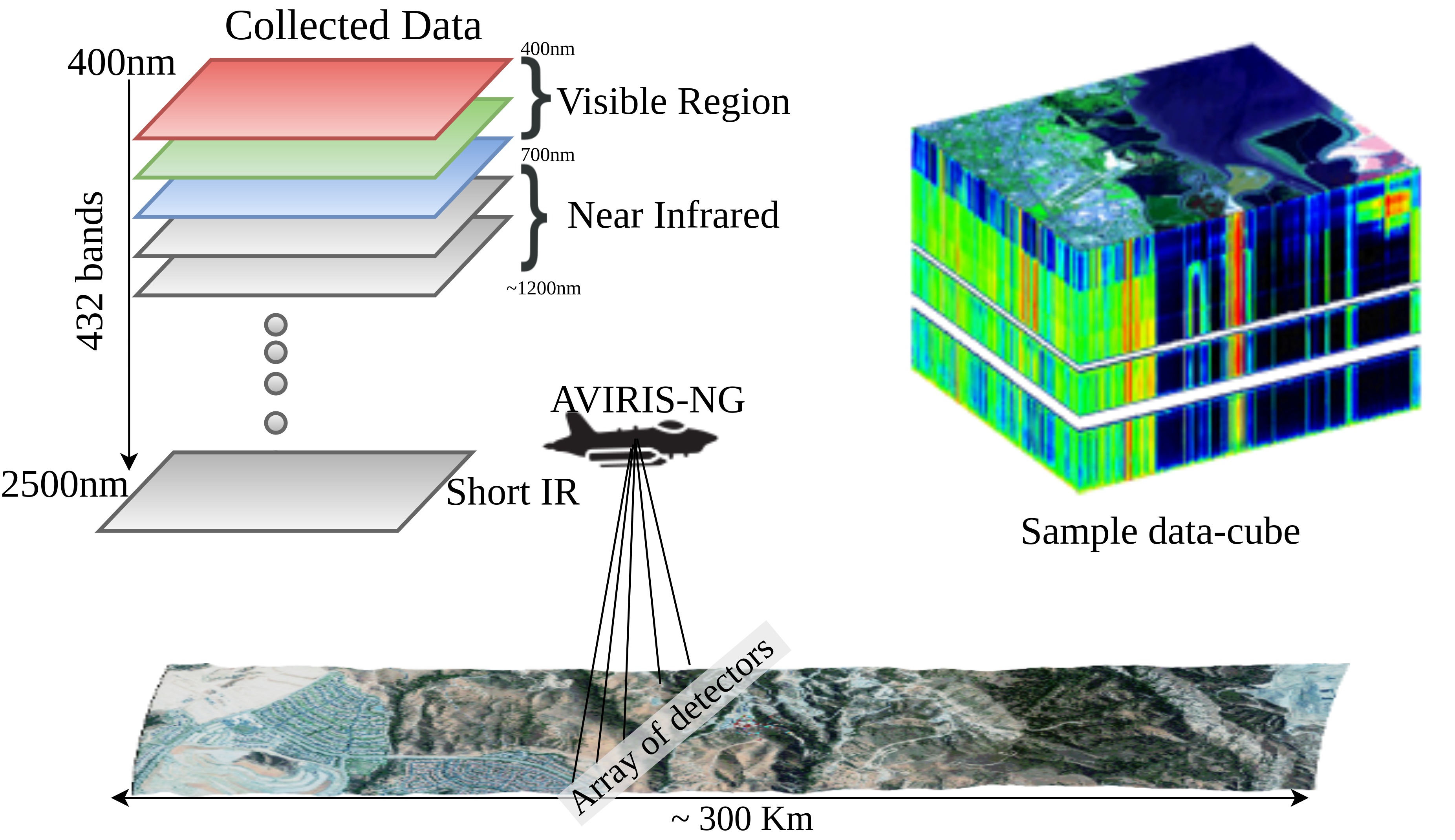
Figure 1: Depiction of data collection process. Each flightline is $\sim 300$ km long. An array of 598 sensors records data at 1.5m/pixel spatial resolution. All flightlines are ortho-corrected. Each data-cube is of dimension $\sim 25000\times\sim 1500\times 432$.

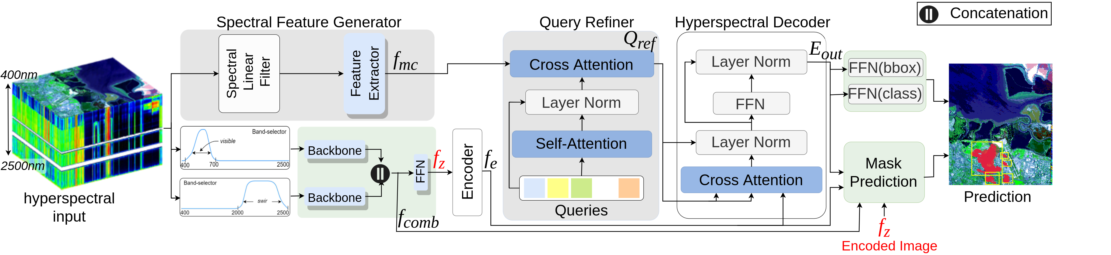
Figure 2: Overview of MethaneMapper (MM) architecture. Given a hyperspectral image, our RGB ($400nm-700nm$) and SWIR ($2000nm-2500nm$) band-pass filters passes a subset of channels in desired wavelength range and feed them to CNN backbones (ResNet) to extract features. These features are concatenated and fed to Transformer Encoder. Parallelly, our Spectral Feature Generator (SFG) modules takes in all channels of input image and generate methane candidates features. Next these candidates are sent to Query Refiner (QR) to refine queries. Then these queries decoded using encoded feature from Transformer Encoder. Finally each decoded query is used to predict a plume mask via Mask Prediction and, bounding box and class via FFNs (Feed Forward Network).

2 Related Works

Our work is at the intersection of hyperspectral data for CH₄ detection, deterministic linear filtering methods for spectral features and encoder-decoder based transformer. A review of the pertinent related works is given below.

There are several recent papers on detecting methane plumes from the airborne imaging spectrometer AVIRIS-NG [22]. This includes the Iterative Maximum a Posterior Differential Optical Absorption Spectroscopy algorithm (IMAP-DOAS) [7, 8] and matched filters [39, 9, 43, 46, 45]. IMAP-DOAS requires data from 2 hyperspectral sensors, one airborne and another on ground, hence not very practical for most application scenarios. Matched-filter based methods use background statistics to normalize the spectral signals and match with the CH₄ spectral signature at every spatial location (pixel-wise). This process, however, is sensitive to surface albedo and land cover with spectral absorption similar to CH₄, leading to spurious detections. Domain experts must then manually inspect each flight line to identify and delineate real CH₄ plumes [44]. To suppress the effect of false positives due to variability of elements on ground, Christopher et.al. [10] and Thorbe et. al. [46] introduced cluster-tuned matched filter. It involves clustering the pixels with similar spectral properties using k-means clustering. Both IMAP-DOAS and all versions of matched filters are heavily prone to false positives as the information is processed pixel-wise.

Machine learning approaches have been used for target detection, including CH₄ identification, in hyperspectral imagery [12, 18, 40, 41, 30]. Similar to matched-filtering, these methods do not take into account the influence of confusers on the CH₄ spectral signature and have similar issues concerning false positives. Recently introduced deep learning based H-mrcnn model [31] focus on capturing spatial correlation. H-mrcnn is an ensemble of mask-rcnncite networks processing blocks of hyperspectral data. This block processing in the spectral domain is inefficient and often results in overall poor performance. Methanet [23] is a more recent work focusing on estimating methane concentration from matched-filter data. In this regard, our proposed MethaneMapper uses both spectral and spatial correlation to accurately delineates CH₄ plumes.

Datasets: The only dataset publicly available with annotation for CH₄ plume detection is JPL-CH₄-detection2017-V1.0 dataset [44]. It contains only 46 AVIRIS-NG [22] flight lines in the US Four-Corners region. Deep learning architectures require a large number of annotated samples, and for this reason we introduce the new MHS dataset with over $1200$ annotated flightlines and $\sim 4000$ plume sites.

3 MethaneMapper (MM) Architecture

3.1 Data Overview

AVIRIS-NG hyperspectral imaging sensors capture spectral radiance values from N₀ (N₀ = 432) channels corresponding to wavelengths ranging from $400nm-2500nm$ as shown in Fig. 1. The complete hyperspectral image is represented as x $\in\mathbb{R}^{H_{0}\times W_{0}\times N_{0}}$ where $H_{0},W_{0}$ are the height & width, respectively, and $N_{0}=432$ is number of channels. This hyperspectral data includes a very weak signature of CH₄ around 2100-2400$nm$, conflated with radiations from the surrounding land cover and background clutter. A single flight-line could be over a couple miles long (about 25K pixels in one of the dimensions), with an array of sensors recording the data at 1.5m/pixel resolution. The images are orthorectified before processing.

3.2 Technical Overview

Referring to Fig.2, MM contains the following main components: (i) 2 CNN backbones to extract a compact feature representation of the spectral regions of interest from the hyperspectral image, (ii) a Spectral Feature Generator (SFG), and (iii) a Query Refiner (QR) in between an encoder-decoder pair (inspired by GTNet [21], SSRT [20]). The hyperspectral image is first processed through two separate band-pass filters to select the channels in visible ($400-700nm$) and short-wave infrared (SWIR)($2000-2500nm$) wavelength regions, and are then passed through CNN backbones. Output of these backbones are concatenated together and then encoded using a transformer encoder.

The SFG (Sec. 3.4) takes in all channels of the hyperspectral image and process them through a spectral linear filter. The SFG exploits the spectral correlation to generate methane candidates feature maps and passes them to QR. The QR (Sec. 3.5) uses these methane candidates to refine the learnable queries. Our hyperspectral decoder takes the encoded features from the encoder and refined queries from QR to generate the embeddings. The mask-prediction layer processes these embeddings along with the feature pyramid from the backbone layers to generate the final methane-plume segmentation prediction.

These individual blocks are discussed in more detail below.

3.3 Bandpass filtering for the Encoder

The HSI is processed by two parallel band-pass filters; a visible wavelength ($400-700nm$) (RGB) and a short-wave infrared wavelength ($2000-2500nm$) (SWIR) band-pass filter. The RGB filter results in a 3 channel output corresponding to the normal red, green, and blue wavelengths. The SWIR generates channels, approximately 5nm apart. The filtered outputs are x_rgb $\in\mathbb{R}^{H_{0}\times W_{0}\times 3}$ and x_swir $\in\mathbb{R}^{H_{0}\times W_{0}\times 100}$. Using x_rgb and x_swir, two conventional CNN backbones (e.g. ResNet-50 [17, 27]) generate two feature maps respectively of size $\in\mathbb{R}^{H\times W\times N}$. Here $H=\frac{H_{0}}{32},\;W=\frac{W_{0}}{32}$ and $N=2048$ typically. We concatenate these feature maps along channel dimension and project through a $1\times 1$ convolution layer to retain channel dimension of $N$. The resulting output is f_comb $\in\mathbb{R}^{H\times W\times N}$.

Following the standard architecture of transformer encoder from previous works [4, 20, 21, 48, 28], we reduce the channel dimension of f_comb using $1\times 1$ convolution to f_z $\in\mathbb{R}^{H\times W\times d}$ and supplement position information by adding a fixed positional embedding p $\in\mathbb{R}^{H\times W\times d}$. The encoder consists of a stack of multi-head self-attention modules and feed-forward networks (FFN). The encoded feature map is f_e $\in\mathbb{R}^{H\times W\times d}$:

$$\textit{f${}_{e}$}=\text{Encoder}(\textit{f${}_{z}$},\textit{p})$$ (1)

3.4 Spectral Feature Generator (SFG)

In parallel, the input hyperspectral image is processed by the SFG module to generate methane candidates feature map f_mc, providing the QR module with spatial information to help the network delineate the methane plumes.

The SFG consist of a spectral linear filter (SLF) and a Feature Extractor (e.g.ResNet-50 [17]). The most common linear filtering approach for detecting CH₄ is to take each pixel from the input hyperspectral image {x_ij $|$ x_ij $\in\mathbb{R}^{1\times 1\times N_{0}}\}$${}_{i,j=1}^{H_{0},W_{0}}$ and project it onto a CH₄ spectral absorption signature vector of same size [13]. This is to reduce the interference from ground terrain and amplify the CH₄ visibility in that pixel. Accurately modeling SLF is critical given that it is designed to reduce ground terrain interference.To model SLF we use the most common approach to matched filtering from information theory [47].

Spectral Linear Filter (SLF):

The design of SLF is dependent on the spectral absorption pattern of CH₄ gas [13] and distribution of ground terrain. Since our signal of interest, CH₄, is very weak, traditional methods of linear filtering [46, 45] are not effective. The conventional methods to whiten the ground terrain noise includes calculating the covariance (Cov $\in\mathbb{R}^{N_{0}\times N_{0}}$) of background by selecting a set of 10-15 adjacent columns {x_i $|$ x_i $\in\mathbb{R}^{1\times H_{0}\times N_{0}}\}$${}_{i=1}^{W_{0}}$). However, in a given flight-line, the terrain changes frequently, from water bodies to bare soil, vegetation, buildings and other urban structures. Therefore single approximation of the covariance can not provide correct estimate of CH₄ and a localized context-based whitening will be more effective. To address this problem, we took a very simple and effective approach of doing land cover classification and segmentation [49, 35, 11], and then compute covariance per class from the land cover. More details in supplementary materials. This improves the quality of methane candidates in presence of confusers (materials with similar spectral absorption patterns as CH₄) and also in cases where CH₄ concentration is low. The final SLF design with per class covariance is:

$$\textbf{SLF}(\textbf{x}_{ij})=\frac{(\textbf{x}_{ij}-\mu_{k})^{T}\textbf{Cov}_{k}^{-1}\textit{t}}{\sqrt{\textit{t}^{T}\textbf{Cov}_{k}^{-1}\textit{t}}}\;\forall\;(i,j)\in\text{class}~{}k$$ (2)

where $t$ represents the spectral absorption pattern [13] of CH₄ gas, and Cov_k, $\mu_{k}$ are the covariance and mean of $k^{th}$ class respectively. x_ij represents the pixel in input hyperspectral image at ($i,j$) index in $k^{th}$ class. This operation generates a 2-D spatial CH₄ candidates map of size $\mathbb{R}^{H_{0}\times W_{0}}$. Next this CH₄ candidates map is fed to a Feature Extractor to generate CH₄ candidates feature map f_mc. Details of the land cover segmentation/classification and complete SLF derivation are in the Supplementary materials.

$$f_{mc}=\text{FeatureExtractor}(\;\textbf{SLF}(\textbf{x}_{ij})\;\forall\;i,j)$$ (3)

3.5 Query Refiner (QR)

Next the methane candidate feature map f_mc $\in\mathbb{R}^{H\times W\times d}$ is fed to the QR module along with a set of $100$ learnable queries Q $\in$ $\mathbb{R}^{100\times d}$. The f_mc refines the learnable queries via cross-attention mechanism. This operation provides a narrow search space for the queries. The QR module follows a transformer decoder-like architecture inspired from [21, 20]. The randomly initialized queries Q $\in\mathbb{R}^{100\times d}$ are first passed through a self-attention layer to attend to themselves. Next, these queries attend to our methane candidates feature map f_mc from SFG module through a cross-attention layer. The methane candidates feature map serves as key-values pairs in our attention architecture. The output of QR is Q_ref.

$$Q_{ref}=\textbf{QR}(f_{mc},Q)$$ (4)

3.6 Hyperspectal Decoder

The Q_ref is fed to the decoder module along with encoder output f_e to generate output embeddings. Our hyperspectral decoder follows the standard architecture with a minor difference. There are no self-attention layers, just stack of multi-headed cross attention layers. The refined queries are transformed into output embeddings E_out $\in\mathbb{R}^{100\times d}$.

$$E_{out}=\text{Decoder}(f_{e},p,Q_{ref})$$ (5)

3.7 Box and Mask Prediction

The decoder output embeddings (E_out) are fed to two Feed Forward Network (FFNs) and a Mask prediction layer. The outputs of the FFNs are the bounding boxes covering each CH₄ plume and a confidence score corresponding to each box. The mask-prediction module follows the standard segmentation head of DETR [4]. It computes multi-head attention scores of each embedding over the f_e (Eq. 1), generating a low-resolution heatmap for each embedding. To make the final prediction a Feature Pyramid Network [15] like structure is used. Each heatmap is designed to capture one methane plume. A simple thresholding is used to merge the heatmaps as final segmentation mask.

$$mask=\text{Mask\_pred}(E_{out},f_{e},f_{comb})$$ (6)

3.8 Training and Inference

We train MethaneMapper in two stages; first we train bounding box detection corresponding to each CH₄ plume, and second by freezing the box detection network and training only the mask prediction module. We also trained both box and mask prediction modules end-to-end and achieved similar performance. We use a similar two-stage loss strategy for training MethaneMapper as that used in DETR [4]: first stage is the bipartite matching between the predictions and the ground truths both in bounding box and mask prediction, and then second stage is loss calculation for the matched pairs. The bipartite matching employs the Hungarian algorithm[4] to find the optimal matching between the predictions and the ground truths. After this matching, every prediction is associated with a ground truth. Next, we calculate the $l_{1}$ and $GIoU$ loss on both box and mask predictions and cross entropy loss for class prediction [4].

Inference:

The inference pipeline is similar to training pipeline and can be implemented using approximately 50 lines of code. During inference, we first filter the detections with confidences below $50\%$ and a per-pixel max to determine which pixels are predicted to belong to a CH4 plume.

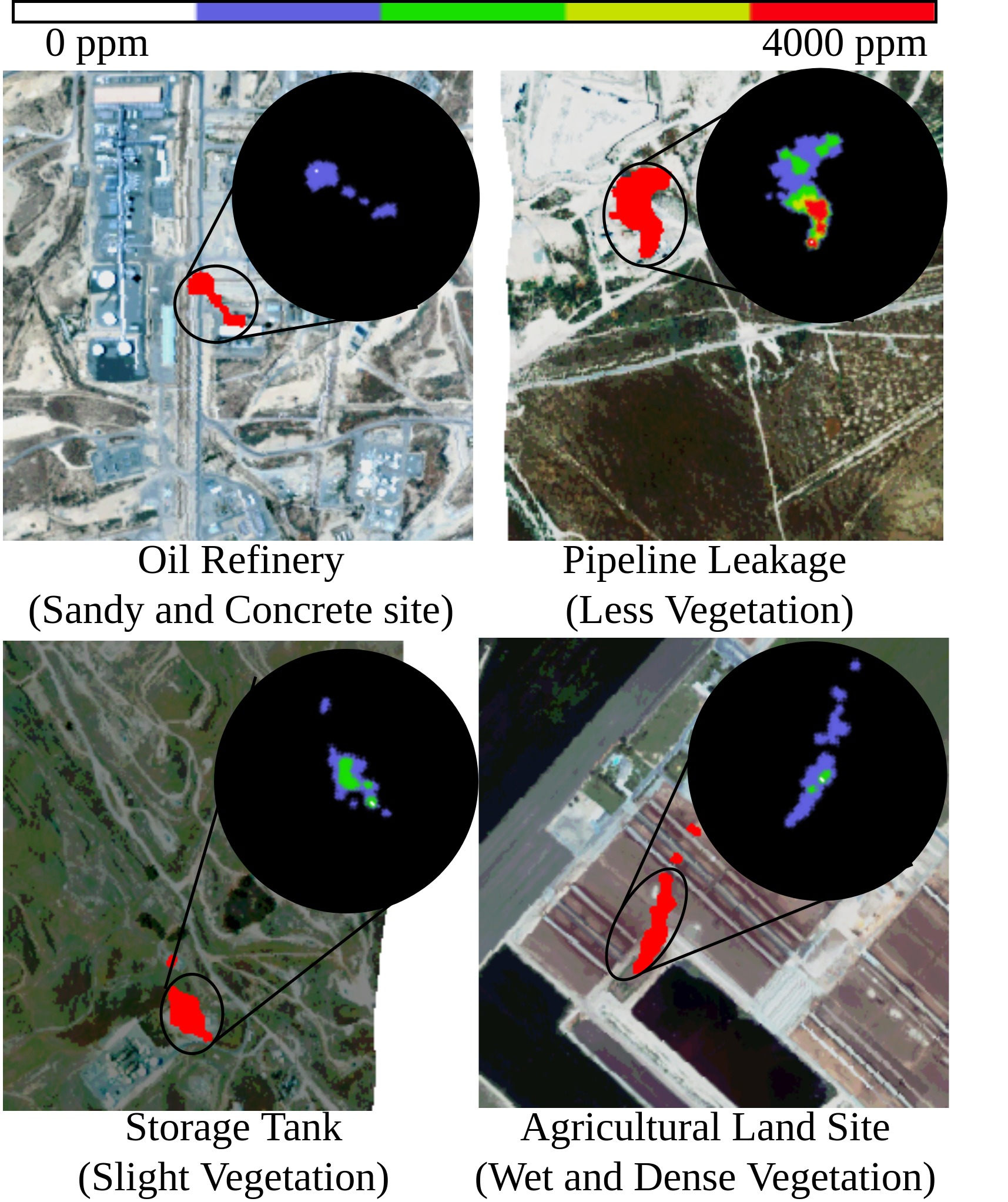
Figure 3: Sample images from MHS dataset. The colormap in black circle shows concentration maps corresponding to the plume mask shown in red. We are showing different types of leakage sources and land cover types. For better visualization, we plotted the binary mask on color image created using visible bands of hyperspectral image.

4 Methane Hot Spots (MHS) dataset

Another significant contribution of this work is a large scale curated MHS dataset. It contains the AVIRIS-NG spectral data with wavelength ranging from $380nm$ to $2510nm$, a $5nm$ sampling [22], and capturing $432$ channels per pixel. The images from the flight-line are orthorectified and of size $\sim 23K\times\sim 1.5K\times 432$. The only currently publicly-available dataset with methane plume segmentation masks is the JPL-CH4-detection-V1.0 [44] dataset released by JPL-NASA in 2017.

The MHS dataset has approximately 4000 plume sites corresponding to approximately 1200 AVIRIS-NG flightlines as shown in Table 1. MHS also has higher diversity data with flight lines spanning from 2015-2022 and covering terrain from 6 states– California, Nevada, New Mexico, Colorado, Midland Texas, and Virginia.

Dataset	MHS (Ours) Dataset	JPL-CH4 detection-V1.0  [44]
# plume sites	3961	161
# flightlines	1185	46
# point source	3675	114
# diffused source	286	57
Time period	2015 - 2022 ( 8 years)	2015 ( 1 year)
Segmentation Mask	Yes	Yes
Bonding box	Yes	No
Concentration map	Yes	No
Number of Regions	6	1

Table 1: Statistics shows MHS dataset comparison with JPL-CH4-detection-V1.0 [44] dataset. Each flightline have multiple large and small plume sites. Each flightline have atleast 4 plume sites. The Point Source represents high concentration ($300kg/hr$) to leakage from sources like pipeline leak, storage tanks, oil and gas refineries. Diffused Source represent low concentration leakages from sources like biomass degradation in landfills. Our dataset is covers more diverse type of terrain over 6 states.

Data Pruning:

We selected AVIRIS-NG flight lines over varying regions as it covers a wide variety of CH₄ plume sources, such as leaks in oil and gas refineries, oil and gas extraction points, natural seeps, leaking underground storage tank, coal mines, dairy farms, landfill sites, and pipeline leaks. Along with varying emission sources, we selected regions with different types of ground terrains like, bare soil, rocks, mountains, light vegetation, water bodies and dense vegetation as shown with few samples in Fig. 3. Different types of ground terrain exhibit widely varying albedo and thus have a major impact on the quality of CH₄ detections as shown in Fig. 4. Given this, training models with diverse ground terrain data leads to a more robust model.

4.1 Concentration map and Segmentation mask

Concentration map is provided in the form of a matrix of spatial dimensions same as the flightline ($\sim 23k\times\sim 1.5k\times 1$). There is one concentration map per flight-line (orthorectified). It shows methane concentration in parts-per-million (ppm) per-pixel on the ground. Pixel-regions with no methane presence are set to zero.

Segmentation mask provided in the format of a “png” image file with three channels and of the same spatial dimension as the corresponding flight line ($\sim 23k\times\sim 1.5k\times 3$). The segmentation mask is obtained from the concentration mask file by setting all pixel values above zero to represent methane plumes. We manually annotated Point Source and Diffused Source based on the type of ground terrain and concentration of methane gas. Following the benchmark dataset [44], three channels are used to color code Point Source (Red) and Diffused Source (Green). The distinction of Point Source and Diffused Source is derived from the JPL-CH4-detection-V1.0 benchmark dataset [44]. Our annotation style is also consistent with the JPL-CH4-detection-V1.0 benchmark dataset [44], so that both datasets can be merged seamlessly.

4.1.1 Constructing Concentration map

Concentration maps are generated by mapping expert-annotated methane-plume concentration maps to the ortho-corrected AVIRIS-NG flightlines. These methane plume annotations are systematically collected from a non-profit [3] entity. They provide concentration masks of methane emissions in $150\times 150$ size patches along with location information from different sources (airborne sensors [6], satellites [38]). In order to map these patches from different sources to the AVIRIS-NG flight-lines, we use the pixel coordinate locations provided for both the annotations and flight-lines. We use this information to create a homography transformation to map each pixel to its corresponding location in the flight-line. Fig. 3 shows a sample of varying types of terrains with CH₄ segmentation mask in red and concentration mask in black circle. Details about matching the resolution, ortho-correction, and transformation are discussed in supplementary materials. The patch annotations are verified by experts visiting the physical location of emission the same day [2]. Most of the regions in California are verified by physical visits by California Air Resource Board [3, 2].

4.2 MHS Statistics

MHS statistics and properties are summarized in Table 1.

Annotations: MHS provides both segmentation masks and concentration maps which enable development of deep learning algorithms than can produce both CH₄ plume location and concentration predictions.

Diversity: MHS dataset includes AVARIS-NG flightlines spanning 8 years (2015 - 2022) from six states in the U.S.: California, Nevada, New Mexico, Colorado, Texas, and Virginia.

Data Split: We divide MHS dataset into train/test splits of 80-20% with overlapping time periods and locations. Our dataset covers 6 states. Each state has sub-regions/locations (e.g. Permian basin) that are covered by multiple non-overlapping flightlines ($25k\times 1.5k\times 432$ pixels). These flightlines are split into train and test sets. In each set, we create patches ($256\times 256\times 432$ pixels) from the corresponding flightlines. From the patches/tiles, we take all positives patches (methane (CH₄)) and randomly sample equal number of negative (no-CH₄) patches. This is done for both train and test sets separately to balance the data and we refer to Section 6.2 for detailed ablation studies.

5 Experimental settings

Evaluation Metrics: Following the evaluation protocol of H-mrcnn [31] we report our performance in mean intersection-over-union (mIOU). Here, mIOU indicates the overlap between the predicted and the ground truth CH₄ plume masks. ED represents the accuracy in plume core prediction. Additionally, as first stage of our two stage training procedure contains bounding box prediction, we also report our performance in predicting plume bounding boxes in terms of mean Average Precision (mAP) which tells us the effectiveness of MethaneMapper in eliminating the false positives in plume prediction.

Data Pre-Processing: Each input hyperspectral image is approximately of size $25000\times 1500\times 432$ taking up memory space of $55-60$ GB. We create tiles of each image in spatial domain, each tile is of size $256\times 256\times 432$ [31] with an overlap of $128$. The CH₄ plume is available in very few pixels in the whole image, $90\%$ of the tiles are negative samples (no methane, just ground terrain). We can not use the whole hyperspectral image because of GPU memory limitations

Implementation Details: The band-selectors module takes 432-channels hyperspectral image as input, the RGB band-selector picks 60 channel from $400nm-700nm$ wavelength range and creates a 3-channel RGB image, the SWIR band-selector picks 100 channel from wavelength range $2000nm-2500nm$. These input images are passed to two ResNet-50 [17] feature extractor backbones. The backbone networks are initialized with DETR [4] trained on COCO dataset [32] and input layer initialized randomly [16]. The transformer encoder-decoder and our query refiner have 6 layers and 8 heads. We initialized the transformer encoder-decoder with weights extracted and stripped from DETR [4] model. The dimension of transformer architecture is $256$ and number of queries is $100$. The SFG module takes in all 432-channels hyperspectral image and generates 1-channel output map of same spatial dimension as input. The feature extractor in SFG is ResNet-50 [17] initialized with DETR [4] trained on COCO dataset [32]. The decoder output embeddings are of size $512$. The feature pyramid network in mask prediction module has 3 layers. More details are mentioned in supplementary materials.

6 Results

In this section we will discuss and validate all the design choices for MethaneMapper (MM) with ablations. We show that MM achieves state-of-the-art results in overall performance compared all other methods shown in Tables 2 & 3.

Methods Back bone SFG F.Ext. #params mAP mIOU JPL-CH4-detection-v1.0 Dataset 1 Hu et. al R-50 - 75M 0.26 0.48 2 H-mrcnn R-50 - 353M 0.53 0.86 3 MM R-50 R-50 80M 0.63 0.91 MHS (Ours) Dataset 4 SpectralFormer R-50 - 84M 0.33 0.41 5 UPSNet (stuff) R-50 - 69M 0.32 0.38 6 UPSNet (stuff + things) R-50 - 69M 0.29 0.35 7 DETR R-18 * 33M 0.37 0.56 8 DETR R-50 * 59M 0.44 0.59 10 R-18 Linear Layer 39M 0.45 0.60 11 R-18 R-18 44M 0.52 0.63 12 MM R-50 R-50 80M 0.59 0.68

Table 2: Comparison with baselines. “-” represent Not Applicable and “*” represent no SFG module and a random query used for transformer decoder. The top section shows performance on JPL-CH₄ dataset [44]. MethaneMapper achieves better results than heavily tuned H-mrcnn with $\sim 5\times$ fewer parameters. The overall detection accuracy is higher on this dataset because the type of ground terrain is uniform across all flightlines. In MHS dataset, MM outperforms multiple baselines as shown in rows 4-12. MM accuracy is lower in MHS than JPL-CH₄ dataset because MHS dataset has more variety of ground terrain spreading over 6 states

Methods mAP mIOU LogReg [5] - 0.05 SVM [40] - 0.29 PCA + LogReg - 0.06 PCA + SVM - 0.31 MM (R-50) 0.63 0.91

Table 3: Comparison with classical machine learning methods. “-” represent Not Available. The classical ML methods are not suited for the CH₄ detection task. MethaneMapper outperforms all methods on JPL dataset [44]

6.1 Performance comparison

Deep Learning methods: We trained MM with ResNet-50 [17] backbone on the same dataset that H-mrcnn [31] (JPL-CH4-detection-V1.0 [44]) was trained on for fair comparison. To align with H-mrcnn we used the same split and input image size. The MM model with $80$M parameters trained for 250 epochs outperforms by significant margin the H-mrcnn model with $352$M parameters. Results are summarized in Table 2 that includes the performance of MM on the new larger MHS dataset. We note that though the code for H-mrcnn is available, many of the modules are deprecated and can not be reproduced. The ’Backbone’ column represents backbones used for feature extraction from input image,’SFG F.Ext.’ represents the feature extractor in SFG module in MethaneMapper. We observed (qualitatively) that H-mrcnn fails to detect small CH₄ plumes with concentration lower than 100kg/hr while MM detects those.

We did evaluation by implementing 3 baseline models [18, 4, 50] shown rows 4-8 of Table 2. These methods were not designed for CH₄ detection task, therefore we needed to modify their input channel size. The poor performance of these methods may be attributed to the weak signal of interest in a high dimensional data, high number of confusers, and limited annotated data. Additionally, the only hyperspectral baseline method SpectralFormer [18] has low efficiency due its pixel-wise training scheme.

Classical ML methods: We trained and tested multiple existing machine learning based approaches that are used for methane detection, performance shown in Table 3. Logistic regression (LogReg) [5] and multinomial logistic regression (MLR) [24] failed to produce any meaningful detection with $90\%$ false positive detections. We also trained a Support Vector Machine (SVM)  [40, 41] based classifier, it performed slightly better than LR and MLR methods with an IOU of 21%. SVMs are prone to false positives detections same as Gaussian Mixture Models [40]. We observed that all traditional methods are not suited for the task of CH₄ detection. We also tested reducing the dimension using principal component analysis (PCA) or just taking bands which shows maximum CH₄ absorption. In the later case, the traditional methods performed better than using all 432 bands, this backs our idea of just using bands from SWIR region.

Qualitative results. Fig. 5 shows comparison of MM’s mask and bounding box prediction with ground truth mask on different ground terrains. The Leakages are from different type of sources such as, oil refinery, pipeline and storage tank. MM makes correct predictions in varying scenarios.

6.2 Ablation Studies

We did the experiments for ablation on MHS dataset with ResNet-50 as backbone and validate the design choices. One parameter is changed for each ablation and others kept at best settings. More ablations in Supplementary.

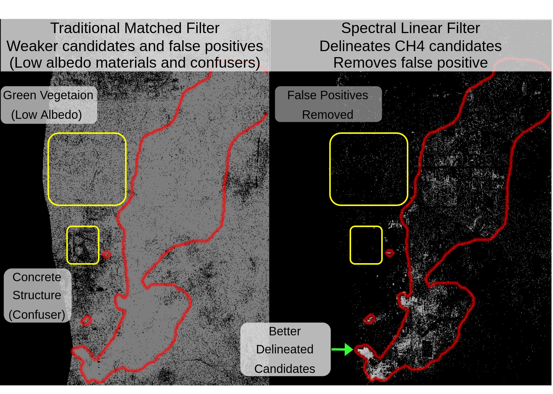
Figure 4: Comparison of SLF with traditional filter in SFG module. White pixels represent methane and black no-methane. Red boundary represents ground-truth plume mask. SLF module generates better CH₄ candidates

Spectral Feature Generator Module:

In Table 2 lower section, we show the effectiveness of our SFG module for the query refiner block. Our baseline is standard implementation of DETR [4] for segmentation task represented by row-1 and row-2 of Tab. 2 lower section. Using CH₄ candidates feature from SFG improves the bounding box detection performance by 0.14 mAP and mask prediction by 0.09 mIOU. This demonstrate that guiding queries with CH₄ candidates feature generated by SFG produces better embeddings as compared to random queries.

Along with this, we explored the provision of CH₄ candidates feature at 2 places, (i) at input level concatenating it with $f_{comb}$; and (ii) as input to query refiner. We see an improvement of 0.09 mAP and 0.08 mIOU when SFG module output is passed to query refiner. We hypothesize that this is because on concatenating with input features, the CH₄ candidates feature information gets lost, while as cross-attention with queries reduces the search space for decoder and generate better embeddings.

We also experimented with different types of feature extractors for SFG module, and observed that a Resnet18 or Resnet50 [17] is more effective than a 2 linear layer feature extractor as shown in Table 2.

Spectral Linear Filter: We experimented with SLF for computing covariance (Cov) using different subset of columns in the input hyperspectral image. We observed that the SLF is most effective when covariance is computed class-wise based on land cover. Class-wise Cov ensures that the radiance absorption by ground terrain is same for all the pixels while computing CH₄ enhancement. As can be seen in Fig. 4, SLF amplifies CH₄ candidate detection and reduces false positives. SLF leads to a 0.03 mAP improved in detection compared to traditional filters. The prediction from MM is shown row-1 of Fig. 5.

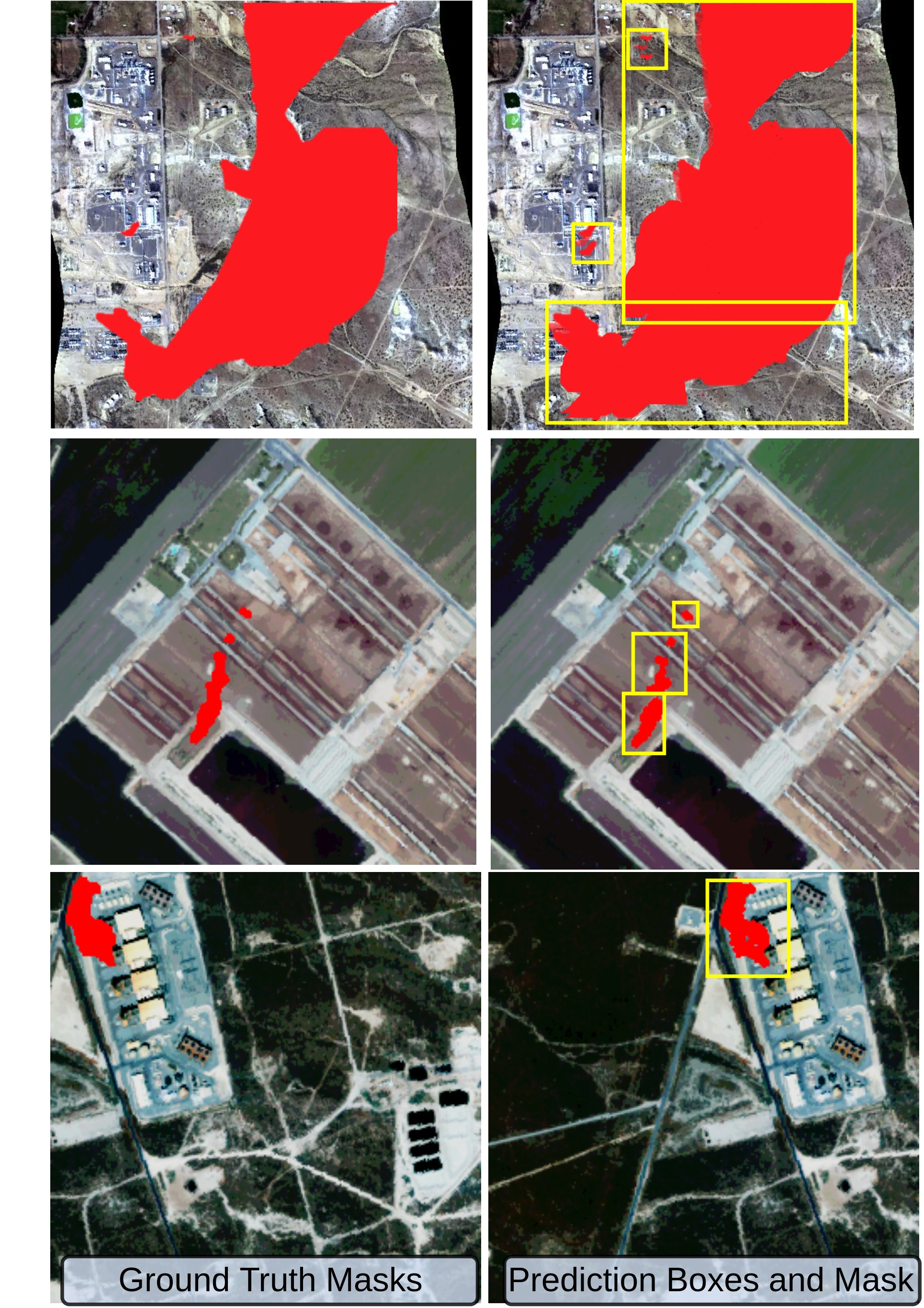
Figure 5: Sample ground truths and predictions on MHS dataset. We show robustness of MethaneMapper predictions on different kind of ground terrain, rows 1 and 3 shows leakage at a refinery, row 2 shows leakage from pipeline in agricultural land, row 4 shows leakage from storage tank with concrete background.

Geographic generalization: To assess the geographical generalization capabilities of MM, we trained it on MHS data from all states except California and tested it on flightlines from California. We observed a slight drop of 0.04 mAP in detections. However, when trained on all data except Virginia, we noticed a significant drop of 0.09 mAP in detections. We attribute this to the fact that the land cover in Virginia is dense and moist vegetation, has a lower solar reflectance compared to the arid regions of California, Texas, and Nevada.

Temporal generalization: Testing MM on 2015 after training on data from 2016-2022 showed no performance drop.

Unbalanced test set: MM’s performance dropped by 0.05 mAP on an unbalanced test set with only 10% positive samples (CH₄) and 90% negative samples (no-CH₄). This highlights the challenges in CH₄ detection. Future work will address this issue.

7 Conclusion

This paper presents MethaneMapper – a hyperspectral Transformer for methane plume detection. It utilize spectral and spatial correlations using a spectral feature generator and a query refiner, to accurately delineate the CH₄ plumes. Additionally, we curated a large-scale dataset for the task, a first of its kind, which will be made available to all researchers. The proposed MethaneMapper significantly improves upon the current methods in terms of detection and localization accuracy, as our extensive experiments demonstrate. Future work will extend the model to global monitoring [29] using multispectral satellite imaging data.

8 Acknowledgments

This research is partially supported by the following grants: NSF award SI2-SSI #1664172 and US Army Research Laboratory (ARL) under agreement number W911NF2020157.

9 SUPPLEMENTARY MATERIALS

In supplementary section, we provide will all the details about the data collection and annotations creation process. We also provide with the complete derivation of Spectral Linear Filter (SLF) along with a pseudo implementation of SLF algorithm. Next in the document we provide some more qualitative examples of success and failure cases of MethaneMapper. Towards the end of the document we provide graph plots about training convergence of all the ablation experiments with Spectral Feature Generator (SFG) and Query Refiner (QR) module.

9.1 Dataset

9.1.1 AVIRIG-NG

AVIRIS-NG [22] is an acronym for the Airborne Visible InfraRed Imaging Spectrometer - Next Generation developed by Jet Propulsion Laboratory (JPL) in 2009. JPL conducted thousands of flight lines recording data with AVIRIS-NG instrument in last 7 years. On the AVIRIS-NG instrument an array of total $598$ sensors in push-broom order captures an unortho-rectified data-cube of spatial dimension $\sim 23k\times 598$, where each sensor records a spectral wavelengths ranging from $380nm-2510nm$  [14] making a dimension of $432$ channels. It has $34^{o}$ field of view with a 1 mrad instantaneous field of view the generates spatial resolution of $1-8m$ based on altitude. This data is then rectified using a geometric lookup table and the resulting data cube is of size $\sim 23k\times\sim 1.5k\times 432$. The data is provided in Band Interleaved by Line (BIL) ordering. BIL ordering signifies the 3D matrix is indexed first by image row, then by channel, and then by the image column [44]. One can find details about the naming convention and the type of data each files contain in “README.txt” file in each flightline folder. The data can be loaded into a $numpy$ array easily using python libraries. All data is orthorectified.

9.1.2 Annotations

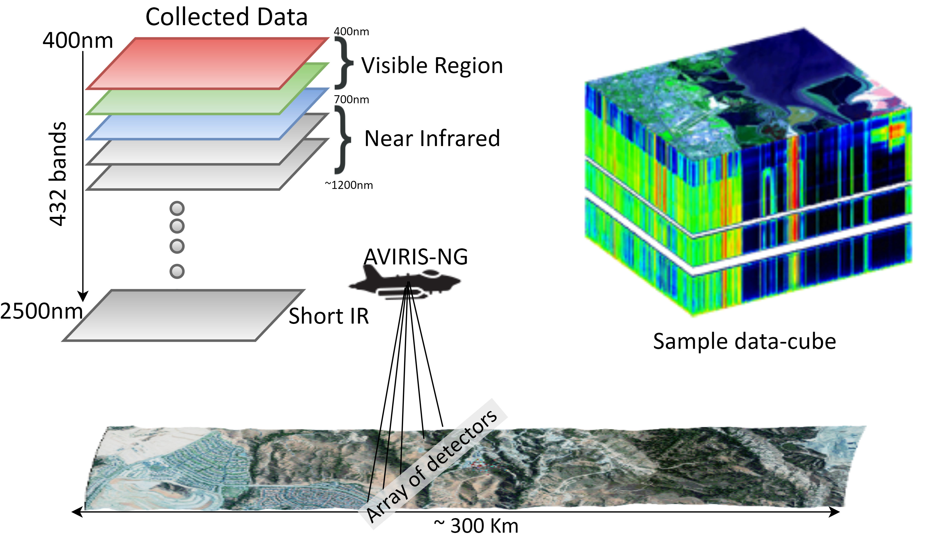
Figure 6: Depiction of data collection process. Each flightline is $\sim 300$ kms long. An array of 598 sensors records data at 1.5m/pixel spatial resolution. All flightlines are ortho-corrected. Each data-cube is of dimension $\sim 23k\times\sim 1.5k\times 432$.

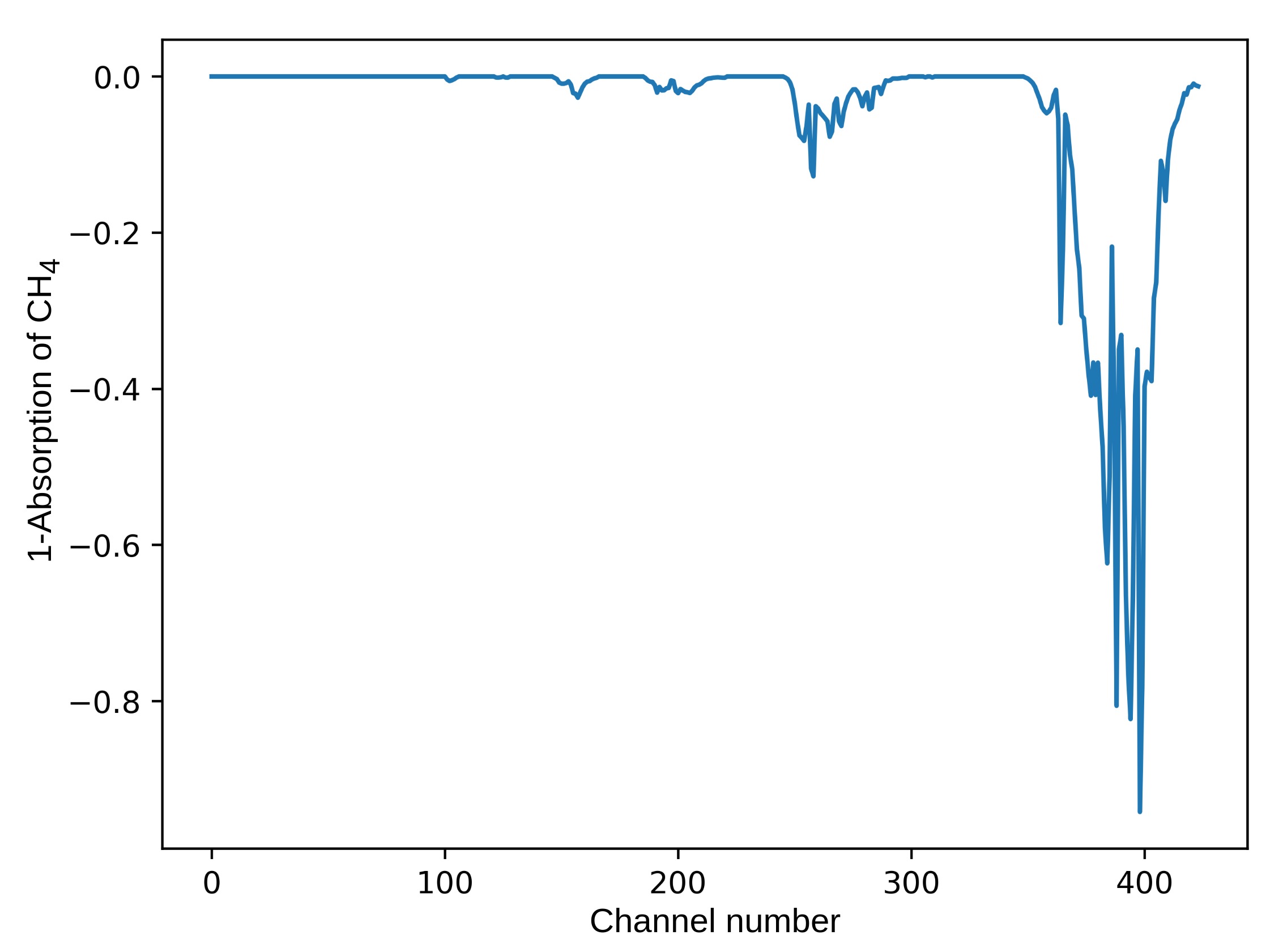
Figure 7: Spectral absorption pattern of CH₄ gas. The x-axis show the channel number ranging from 0-400 corresponding to wavelength range ($400nm-2500nm$). It is obtained from the public repository HITRAN [13].

Transformation and Ortho-correction. First step is to read the annotation GeoTiff patch of size $150\times 150$ of a methane concentration mask and convert its Coordinate Reference System (CRT) to AVIRIS-NG flightlines’ CRT (EPSG 4326). Next, we use the corresponding AVIRIS-NG flightlines’ geometric lookup table and unortho-corrected geographic pixel location to generate ortho-corrected geographic pixel location data of the flightline. Next, we find the flightline’s geographic indices that are closest to the geographic indexes of the methane concentration mask (annotation GeoTiff). Finally, we use these corresponding pixels to compute a homography transform matrix that maps the methane concentration mask (annotation GeoTiff) to the AVIRIS-NG flightline’s spatial dimensions. We repeat this process for each plume in the flightline in order to generate the CH₄ concentration map for the entire flightline.

Resolution matching. To match the resolution of transformed annotation GeoTiff patch to AVIRIS-NG flightline, we use nearest-neighbor resampling. A pixel from the transformed annotation GeoTiff patch may be repeated multiple times in the CH₄ concentration map for the entire flightline.

Annotation Style. The Point Source and Diffused Source are coded following the same standard as JPL-CH4-detection-V1.0 [44] dataset. The 3-channels have values in [0-255] range.

• Red (255,0,0): plume, believed to be associated with a Point Source

• Blue (0,0,255): plume, believed to be associated with a Diffuse Source

• Black (0,0,0): no plume (or unlabeled)

We kept our annotation style consistent with JPL-CH4-detection-V1.0 benchmark dataset [44] so that both JPL-CH4-detection-V1.0 and MHS datasets can be merged seamlessly.

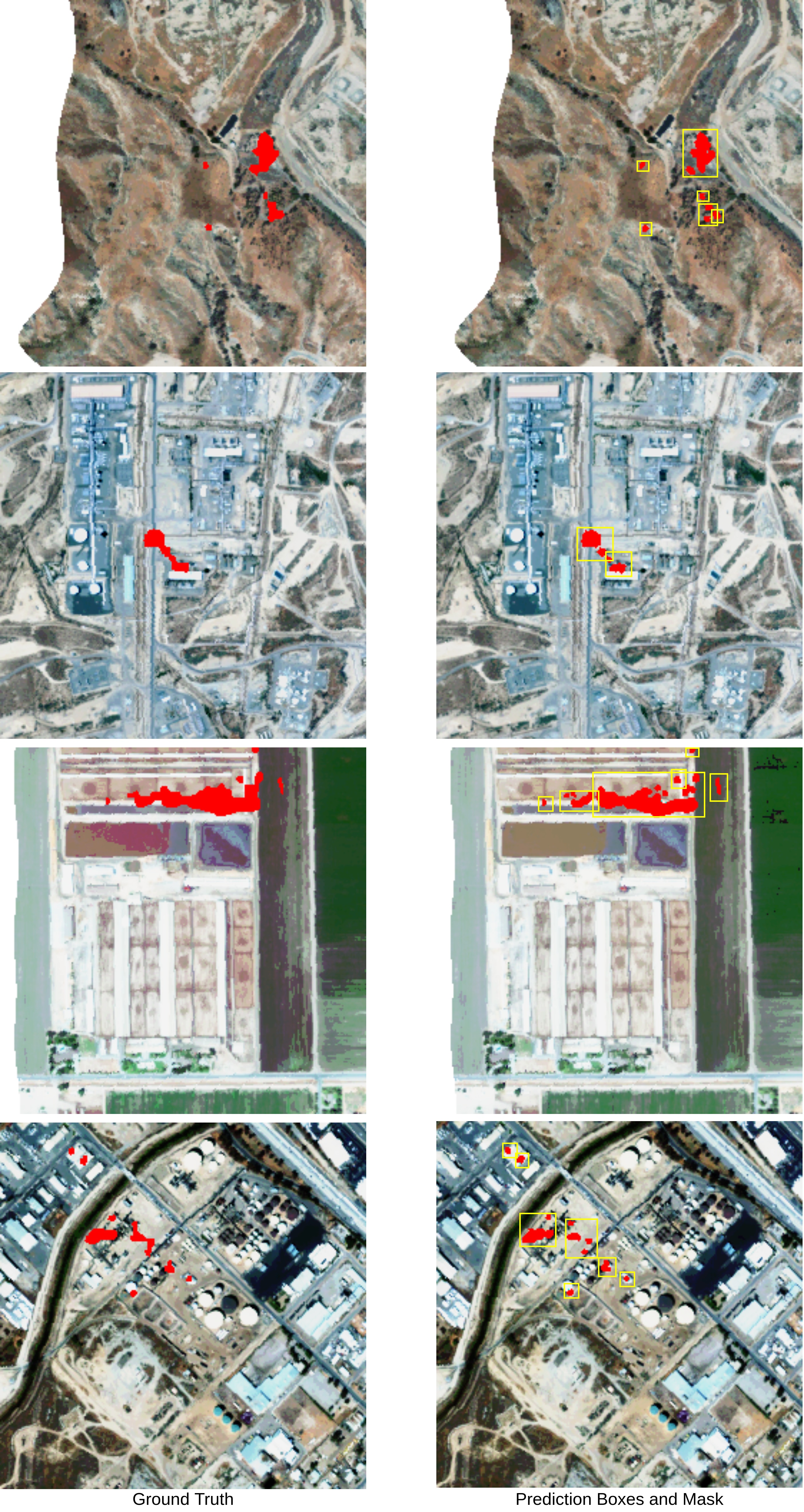
Figure 8: Sample ground truths and predictions on MHS dataset. We are showing different type of terrains and CH₄ predictions on them. The type of emission source in all samples varies too.

9.2 Spectral Linear Filter(SFL)

9.2.1 Traditional Matched Filter

Passive hyperspectral imaging sensors captures spectral radiances values from $N_{0}$ ($N_{0}=432$) spectral channels corresponding to wavelengths ranging from $400nm-2500nm$ as shown in Fig. 6 with sample data-cube. The complete hyperspectral image is represented as x $\in\mathbb{R}^{H_{0}\times W_{0}\times N_{0}}$ where $H_{0},W_{0}\&N_{0}$ are height, width and number of channels respectively. In this hyperspectral data, we are looking for a very weak signature of interest hidden in background. In this case the signature of interest is CH₄ and the background is ground terrain. CH₄ shows strong absorption patterns around $2100nm-2500nm$ wavelength.

The most common linear approach for finding CH₄ candidates is taking a $N_{0}$-dimension (same as number of spectral channels) vector $\alpha$, and apply as a dot product to each pixel ($N_{0}$-dimension) in the hyperspectral image to generate a scalar output per pixel. This operation is supposed to reduce or remove the ground terrain, sensor noise and amplifies CH₄ signature. The $\alpha$ vector used here is called as “matched filter”. Therefore computing right $\alpha$ is very critical for generating better candidates of CH₄ emission. It is dependent on absorption pattern of CH₄ and on the distribution of the ground terrain. To model $\alpha$, let $\textbf{r}_{i}\in\ \mathbb{R}^{n}$ be a $i^{th}$ pixel from the hyperspectral image representing the ground terrain pixel and sensor noise, and t be the CH₄ absorption pattern [13]. This is modeled as the additive perturbation as shown below:

$$\textbf{x}_{i}=\textbf{r}_{i}+\textbf{t},$$ (7)

where $\textbf{x}_{i}$ is the spectrum when CH₄ is present. The CH₄ absorption pattern t represents the change in radiance units of the background caused by adding a unit mixing ratio length of CH₄ absorption [10, 31]. Figure 7 shows the spectral absorption pattern of CH₄ per channel. In the ideal scenario where only CH₄ gas is present in signal (i.e. all white background), the matched filter output is $\alpha^{T}\textbf{t}$. In case there is no gas and just ground terrain and sensor noise, the matched filter output is $\alpha^{T}\textbf{r}_{i}$. The variance ($Var$) of $\alpha^{T}\textbf{r}_{i}$ for latter is represented by:

$$Var(\alpha^{T}\textbf{r}_{i})=\langle(\alpha^{T}\textbf{r}_{i}-\alpha^{T}\boldsymbol{\mu})^{2}\rangle=\alpha^{T}\textbf{Cov}\alpha,$$ (8)

where Cov and $\mu$ are covariance and mean respectively computed for $\textbf{r}_{i}$. Inspired from [31, 10] we define the Methane-to-Ground terrain Ratio (MGR) is:

$$\text{MGR}=\frac{|\alpha^{T}\textbf{t}|^{2}}{\alpha^{T}\textbf{Cov}\alpha},$$ (9)

We can see that the magnitude of $\alpha$ does not affect MGR. According to [42, 10, 31], the MGR can be maximized subject to constraints(zero mean and $\alpha^{T}\textbf{K}\alpha$ constraint to 1). The matched filter $\alpha$ is then represented by:

$$\alpha=\frac{\textbf{Cov}^{-1}\textbf{t}}{\sqrt{\textbf{t}^{T}\textbf{Cov}^{-1}\textbf{t}}}.$$ (10)

In ideal instances when there is no background (i.e. all white background) and just CH₄ gas present. The matched filter in equation 11 is directly proportional to t. This is just the target signature (t) itself scaled so that the filtered output has variance of one. The methane enhancement per pixel can be computed as follows:

$$\hat{\alpha}(\textbf{x}_{i})=\frac{(\textbf{x}_{i}-\mu)^{T}\textbf{Cov}^{-1}\textbf{t}}{\sqrt{\textbf{t}^{T}\textbf{Cov}^{-1}\textbf{t}}},$$ (11)

where $\hat{\alpha}(\textbf{x}_{i})$ is the per pixel estimation of methane, on other words, column enhancement of methane. The covariance matrix (Cov) used is not known as $prior$ and is estimated from data. It is computed as outer product of the mean subtracted radiance over all the pixels. In other words, the traditional matched filter from equation 11 computes the covariance (Cov) of ground terrain with an underlying assumption that in all elements have similar absorption pattern. Same covariance matrix (Cov) matrix is used to whitens the varying ground terrain and amplify the CH₄ present. But in realistic scenarios, the ground terrain is varying, the type of terrain changes frequently, there is water bodies, bare soil, vegetation, dense vegetation, building structures in cities, roads etc in a single image. For example, water have a strong absorption of solar radiations, therefore the methane on such backgrounds have a very weak visibility. Similarly, wet fields dense vegetation have similar behaviour. On the other hand, bare soil, rocks, etc have lower absorption, the methane present on such background have strong visibility. A simple and single approximation of the covariance (Cov) of ground distribution can not provide the right and effective estimate of methane enhancement. To tackle this limitation, we developed an spectral linear Filter (SLF) that does land cover classification and segmentation and reduces the noise as discussed in the next sections.

9.2.2 Landcover Classification and Segmentation

In this section, we improve upon the limitations mentioned in the previous section. We start with taking hyperspectral bands from visible spectrum ($400nm-700nm$) and near-mid infrared region ($800nm-1350nm$). We recreated the $RGB$ representation of the ground terrain by a weighted normal distribution for each color band. Same is done for near infrared region. Next we take a simple, very effective and efficient approach for doing landcover classification and segmentation. We compute the Normalized Difference Vegetation Index (NDVI) [37, 35] and Normalized Difference Water Index (NDWI) [11]. NDVI quantifies vegetation by measuring the difference between near-infrared (which vegetation strongly reflects) and red light (which vegetation absorbs) [35]. It ranges from $-1$ to $+1$. It is a very effective index and has been used in literature for more than 4 decades.  [11] created NDWI and used it to highlight open water features in a satellite image, allowing a water body to “stand out” against the soil and vegetation. It is calculated using the GREEN-NIR (visible green and near-infrared) and ranges from $-1$ to $+1$. Its primary use today is to detect and monitor slight changes in water content of the water bodies.

$$ndvi=\frac{NIR-R}{NIR+R};\;\;ndwi=\frac{NIR-MIR}{NIR+MIR}$$ (12)

where $NIR$ is near infrared region normalized around $880nm$, $MIR$ is mid infrared normalized around $1240nm$ and $R$ is red, normalized around $660nm$. We take advantage of these indexes and create segmentation maps for different types of vegetation, water bodies, bare soil, rocks, mountains, city/urban areas, roads etc. We take the classification thresholds from [26, 49]. For simplification, we also tested by splitting the scale $-1$ to $+1$ in 20 classes, each with a range of $<0.1>$. We obtained comparable results as compared to using classification ranges from [26, 49]. This simple, effective and efficient approach gives three fold boost to our spectral linear filter CH₄ candidates estimation.

9.2.3 Cov per class

We take the segmented image from previous step, we will call segmented image as segmentation mask for simplicity now onward. In practice we have 20 classes, each with a segmentation mask. We merged two or more adjacent classes into one if the number of pixels in that class is less $10000$ . The Number of pixels in each class is kept higher to ensure that while computing the covariance (Cov) matrix, the methane signal does not have any or have negligible effect. It is okay to merge adjacent classes into one because they have almost similar radiance/reflectance, for example, light vegetation and normal vegetation have similar reflectance, etc. For each class we compute a separate mean and covariance matrix. The covariance $\textbf{Cov}_{k}$ of $k^{th}$ class is computed as:

$$\textbf{Cov}_{k}=\frac{1}{N}\sum_{i=1}^{i=j}(\textbf{x}_{i}-\mu_{k})(\textbf{x}_{i}-\mu_{k})^{T}\;\forall\;j\in k,$$ (13)

where $N$ is the number of pixels ($>10000$) in $k^{th}$ class and $\mu_{k}$ is the mean of $k^{th}$ class. For each class we compute the mean $\mu_{k}$, covariance matrix $\textbf{Cov}_{k}$. While iterating through each pixel of hyperspectral image, we check to which class $k$ the pixel $\textbf{x}_{i}$ belongs to and use those pre-computed values. The final Spectral Linear Fitler (SLF) is shown as below:

$$\textbf{SLF}(\textbf{x}_{i})=\frac{(\textbf{x}_{i}-\mu_{k})^{T}\textbf{Cov}_{k}^{-1}\textit{t}}{\sqrt{\textit{t}^{T}\textbf{Cov}_{k}^{-1}\textit{t}}}\;\forall\;(i)\in\text{class}~{}k$$ (14)

where $\textbf{Cov}^{-1}$ is the inverse of covariance matrix. Next to suppress the sensor noise, we exploit the simple method of tracking each sensor. Each sensor have different physical properties, that can influence the data captured by it. We track each individual sensor in the flight line. Since the data is rectified, the data from each sensor does not belong to single column, instead it is spread randomly across all the columns. This is dependent on the flight path and the movement in the airplane while moving. We used simple data-structure algorithms like depth first search. Tracked each boundary pixels and assigned them to single sensor. We used data from 10-15 adjacent sensor at one time, normalize it and then compute the covariance matrix in previous step with segmentation mask. Our approach is very simple and straight forward.

The algorithm 1 shows the pseudo code for our Spectral Linear Filter (SLF).

Data: MHS dataset

Result: CH₄ concentration map

initialization;

for $mhs$ in $MHS$ do

       1. create memory map $mhs$;

       2. seg_mask = compute segmentation mask;

       for mask in seg_mask do

             data.append($mhs$[mask])

             if (len(data) $<100000$): continue

             Cov, $\mu$ = compute_stats(data);

            

       end for

      3. sensor_array = individual sensors;

       for arrays in sensor_array do

             data = $mhs$[arrays]

             for x_i in data do

                   k = seg_mask[i];

                   $\textbf{SLF}(\textbf{x}_{i})=\frac{(\textbf{x}_{i}-\mu_{k})^{T}\textbf{Cov}^{-1}_{k}\textbf{t}}{\sqrt{\textbf{t}^{T}\textbf{Cov}^{-1}_{k}\textbf{t}}}$

                  

             end for

            

       end for

      $\textbf{SLF}(\textbf{x}_{i})\;\forall\;classes\;and\;i\in mhs$

end for

Algorithm 1 Enhanced Matched Filter

9.2.4 Training policy

We trained MethaneMapper in two styles, (i) pre-training the bounding box and class detection first and then freezing the pre-trained model parameters and training only the mask prediction layer; and (ii) trained whole pipeline end-to-end and achieved similar performance on both the cases.

9.2.5 Qualitative Results

In this section we show few more qualitative examples of CH₄ plume mask prediction and few cases where MM failed to detect any CH₄ gas emission.Figure. 8 shows the CH₄ detections in different types of background terrain and different types of emission source.

Figure 9 shows some examples of missed CH₄ plume detections. We observed that going back to dataset samples and checking the timelines, these flightlines were recorded during the evening time. We believe that this might be because of evening time, the reflectance from the ground terrain is very weak and small. Hence we believe there is minimum absorption of reflected solar radiation by CH₄ gas present in the atmosphere and the plume goes undetected.

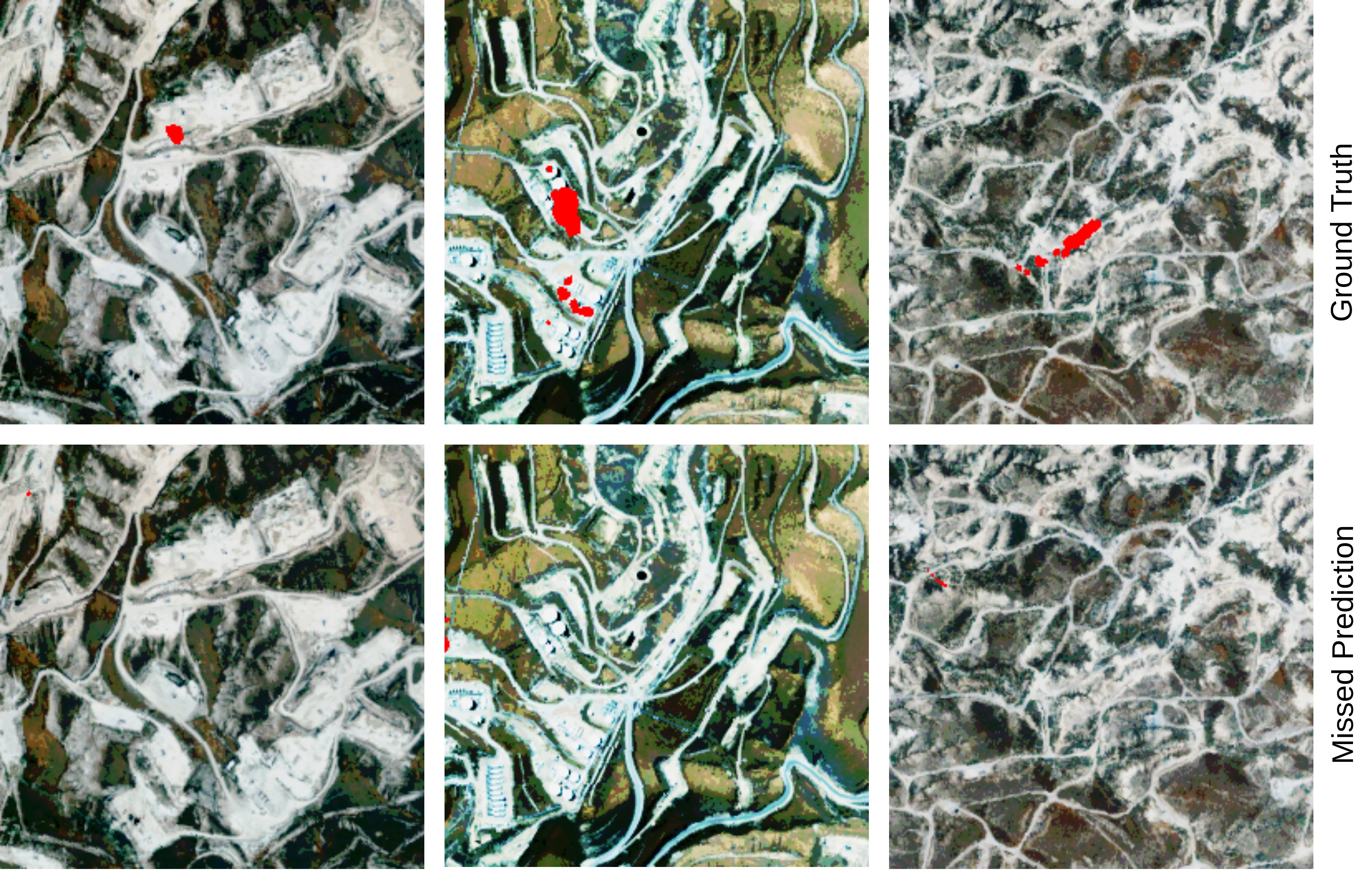
Figure 9: Samples where MM fails to detect the CH₄ plume. We observed that these samples were recorded during the evening time and hence reflectance from the ground terrain is very weak. Therefore the absorption of reflected solar radiations by CH₄ is very low and hence the emissions goes undetected.

9.3 Ablations Studies

Attention Type: We also explored different attention mechanisms to encode and decode information. We replaced only the attention layers with deformable-attention [51] in the our architecture that resulted in a drop of 0.1 mAP in the baseline model.

9.3.1 Implementation details

The whole network is trained with AdamW [33] optimizer, batch size of 12, with initial learning rate for backbones set to $10^{-5}$ and for transformer the learning rate is set to $10^{-5}$ with a weight decay of $10^{-4}$. The learning rate for mask prediction module is set to $10^{-4}$. The learning rate is dropped at every 150 epochs, we train for 300 epochs. The baseline model is trained on 2 V100 GPUs.

References

- [1] Alana K. Ayasse, Andrew K. Thorpe, Dar A. Roberts, Christopher C. Funk, Philip E. Dennison, Christian Frankenberg, Andrea Steffke, and Andrew D. Aubrey. Evaluating the effects of surface properties on methane retrievals using a synthetic airborne visible/infrared imaging spectrometer next generation (aviris-ng) image. Remote Sensing of Environment, 215:386–397, 2018.
- [2] CALIFORNIA AIR RESOUCE BOARD. Green house gas inventory by california air resource board, 2022.
- [3] INC CARBON MAPPER. Carbon mapper methane emission exploration, 2022.
- [4] Nicolas Carion, Francisco Massa, Gabriel Synnaeve, Nicolas Usunier, Alexander Kirillov, and Sergey Zagoruyko. End-to-end object detection with transformers. In European conference on computer vision, pages 213–229. Springer, 2020.
- [5] Qi Cheng, Pramod K Varshney, and Manoj K Arora. Logistic regression for feature selection and soft classification of remote sensing data. IEEE Geoscience and Remote Sensing Letters, 3(4):491–494, 2006.
- [6] E. Knapp David, Heckler Joseph, Seely Megs, and P. Asner Gregory. Global airborne observatory visible to infrared imaging spectrometer report, 2020.
- [7] C Frankenberg, U Platt, and T Wagner. Iterative maximum a posteriori (imap)-doas for retrieval of strongly absorbing trace gases: Model studies for ch 4 and co 2 retrieval from near infrared spectra of sciamachy onboard envisat. Atmospheric Chemistry and Physics Discussions, 4(5):6067–6106, 2004.
- [8] Christian Frankenberg, U Platt, and T Wagner. Iterative maximum a posteriori (imap)-doas for retrieval of strongly absorbing trace gases: Model studies for ch 4 and co 2 retrieval from near infrared spectra of sciamachy onboard envisat. Atmospheric Chemistry and Physics, 5(1):9–22, 2005.
- [9] Christian Frankenberg, Andrew K Thorpe, David R Thompson, Glynn Hulley, Eric Adam Kort, Nick Vance, Jakob Borchardt, Thomas Krings, Konstantin Gerilowski, Colm Sweeney, et al. Airborne methane remote measurements reveal heavy-tail flux distribution in four corners region. Proceedings of the national academy of sciences, 113(35):9734–9739, 2016.
- [10] Christopher C Funk, James Theiler, Dar A Roberts, and Christoph C Borel. Clustering to improve matched filter detection of weak gas plumes in hyperspectral thermal imagery. IEEE transactions on geoscience and remote sensing, 39(7):1410–1420, 2001.
- [11] Bo-Cai Gao. Ndwi—a normalized difference water index for remote sensing of vegetation liquid water from space. Remote sensing of environment, 58(3):257–266, 1996.
- [12] Utsav B Gewali, Sildomar T Monteiro, and Eli Saber. Machine learning based hyperspectral image analysis: a survey. arXiv preprint arXiv:1802.08701, 2018.
- [13] IE Gordon, LS Rothman, RJ Hargreaves, R Hashemi, EV Karlovets, FM Skinner, EK Conway, C Hill, RV Kochanov, Y Tan, et al. The hitran2020 molecular spectroscopic database. Journal of quantitative spectroscopy and radiative transfer, 277:107949, 2022.
- [14] L. Hamlin, R. O. Green, P. Mouroulis, M. Eastwood, D. Wilson, M. Dudik, and C. Paine. Imaging spectrometer science measurements for terrestrial ecology: Aviris and new developments. In 2011 Aerospace Conference, pages 1–7, 2011.
- [15] Kaiming He, Georgia Gkioxari, Piotr Dollár, and Ross Girshick. Mask r-cnn. In Proceedings of the IEEE international conference on computer vision, pages 2961–2969, 2017.
- [16] Kaiming He, Xiangyu Zhang, Shaoqing Ren, and Jian Sun. Delving deep into rectifiers: Surpassing human-level performance on imagenet classification. In Proceedings of the IEEE international conference on computer vision, pages 1026–1034, 2015.
- [17] Kaiming He, Xiangyu Zhang, Shaoqing Ren, and Jian Sun. Deep residual learning for image recognition. In Proceedings of the IEEE conference on computer vision and pattern recognition, pages 770–778, 2016.
- [18] Danfeng Hong, Zhu Han, Jing Yao, Lianru Gao, Bing Zhang, Antonio Plaza, and Jocelyn Chanussot. Spectralformer: Rethinking hyperspectral image classification with transformers. IEEE Transactions on Geoscience and Remote Sensing, 60:1–15, 2021.
- [19] Paris IEA. Methane from oil & gas, 2020.
- [20] ASM Iftekhar, Hao Chen, Kaustav Kundu, Xinyu Li, Joseph Tighe, and Davide Modolo. What to look at and where: Semantic and spatial refined transformer for detecting human-object interactions. In Proceedings of the IEEE/CVF Conference on Computer Vision and Pattern Recognition, pages 5353–5363, 2022.
- [21] ASM Iftekhar, Satish Kumar, R Austin McEver, Suya You, and BS Manjunath. Gtnet: Guided transformer network for detecting human-object interactions. arXiv preprint arXiv:2108.00596, 2021.
- [22] California Institute of Technology Jet Propulsion Laboratory. Airborne visible infrared imaging spectrometer - next generation (aviris-ng) overview, 2009.
- [23] Siraput Jongaramrungruang, Andrew K Thorpe, Georgios Matheou, and Christian Frankenberg. Methanet–an ai-driven approach to quantifying methane point-source emission from high-resolution 2-d plume imagery. Remote Sensing of Environment, 269:112809, 2022.
- [24] Mahdi Khodadadzadeh, Jun Li, Antonio Plaza, and José M Bioucas-Dias. A subspace-based multinomial logistic regression for hyperspectral image classification. IEEE Geoscience and Remote Sensing Letters, 11(12):2105–2109, 2014.
- [25] Stefanie Kirschke, Philippe Bousquet, Philippe Ciais, Marielle Saunois, Josep G Canadell, Edward J Dlugokencky, Peter Bergamaschi, Daniel Bergmann, Donald R Blake, Lori Bruhwiler, et al. Three decades of global methane sources and sinks. Nature geoscience, 6(10):813–823, 2013.
- [26] FJ Kriegler, WA Malila, RF Nalepka, and W Richardson. Preprocessing transformations and their effects on multispectral recognition. Remote sensing of environment, VI, page 97, 1969.
- [27] Satish Kumar, ASM Iftekhar, Michael Goebel, Tom Bullock, Mary H MacLean, Michael B Miller, Tyler Santander, Barry Giesbrecht, Scott T Grafton, and BS Manjunath. Stressnet: detecting stress in thermal videos. In Proceedings of the IEEE/CVF Winter Conference on Applications of Computer Vision, pages 999–1009, 2021.
- [28] Satish Kumar, ASM Iftekhar, Ekta Prashnani, and BS Manjunath. Locl: Learning object-attribute composition using localization. arXiv preprint arXiv:2210.03780, 2022.
- [29] Satish Kumar, William Kingwill, Orbio Earth, Rozanne Mouton, Wojciech Adamczyk, Robert Huppertz, and Evan Sherwin. Guided transformer network for detecting methane emissions in sentinel-2 satellite imagery.
- [30] Satish Kumar, Rui Kou, Henry Hill, Jake Lempges, Eric Qian, and Vikram Jayaram. In-situ water quality monitoring in oil and gas operations. arXiv preprint arXiv:2301.08800, 2023.
- [31] Satish Kumar, Carlos Torres, Oytun Ulutan, Alana Ayasse, Dar Roberts, and BS Manjunath. Deep remote sensing methods for methane detection in overhead hyperspectral imagery. In Proceedings of the IEEE/CVF Winter Conference on Applications of Computer Vision, pages 1776–1785, 2020.
- [32] Tsung-Yi Lin, Michael Maire, Serge Belongie, James Hays, Pietro Perona, Deva Ramanan, Piotr Dollár, and C Lawrence Zitnick. Microsoft coco: Common objects in context. In European conference on computer vision, pages 740–755. Springer, 2014.
- [33] Ilya Loshchilov and Frank Hutter. Decoupled weight decay regularization. arXiv preprint arXiv:1711.05101, 2017.
- [34] META-STANFORD. Methane emissions technology alliance (meta), stanford natural gas initiative, 2022.
- [35] MGISGeography. Ndvi (normalized difference vegetation index), 1979.
- [36] Gunnar Myhre, Drew Shindell, and Julia Pongratz. Anthropogenic and natural radiative forcing. 2014.
- [37] Nathalie Pettorelli. The normalized difference vegetation index. Oxford University Press, 2013.
- [38] Darius Phiri, Matamyo Simwanda, Serajis Salekin, Vincent R Nyirenda, Yuji Murayama, and Manjula Ranagalage. Sentinel-2 data for land cover/use mapping: a review. Remote Sensing, 12(14):2291, 2020.
- [39] Dar A Roberts, Eliza S Bradley, Ross Cheung, Ira Leifer, Philip E Dennison, and Jack S Margolis. Mapping methane emissions from a marine geological seep source using imaging spectrometry. Remote Sensing of Environment, 114(3):592–606, 2010.
- [40] CA Shah, PK Varshney, and MK Arora. Ica mixture model algorithm for unsupervised classification of remote sensing imagery. International Journal of Remote Sensing, 28(8):1711–1731, 2007.
- [41] David MJ Tax and Robert PW Duin. Support vector data description. Machine learning, 54(1):45–66, 2004.
- [42] James Theiler, Bernard R Foy, and Andrew M Fraser. Beyond the adaptive matched filter: nonlinear detectors for weak signals in high-dimensional clutter. In Algorithms and Technologies for Multispectral, Hyperspectral, and Ultraspectral Imagery XIII, volume 6565, pages 26–37. SPIE, 2007.
- [43] DR Thompson, I Leifer, H Bovensmann, M Eastwood, M Fladeland, C Frankenberg, K Gerilowski, RO Green, S Kratwurst, T Krings, et al. Real-time remote detection and measurement for airborne imaging spectroscopy: a case study with methane. Atmospheric Measurement Techniques, 8(10):4383–4397, 2015.
- [44] David R Thompson, Anuj Karpatne, Imme Ebert-Uphoff, Christian Frankenberg, Andrew K Thorpe, Brian D Bue, and Robert O Green. Isgeo dataset jpl-ch4-detection-2017-v1. 0: A benchmark for methane source detection from imaging spectrometer data. 2017.
- [45] Andrew K Thorpe, Christian Frankenberg, David R Thompson, Riley M Duren, Andrew D Aubrey, Brian D Bue, Robert O Green, Konstantin Gerilowski, Thomas Krings, Jakob Borchardt, et al. Airborne doas retrievals of methane, carbon dioxide, and water vapor concentrations at high spatial resolution: application to aviris-ng. Atmospheric Measurement Techniques, 10(10):3833–3850, 2017.
- [46] Andrew K Thorpe, Dar A Roberts, Eliza S Bradley, Christopher C Funk, Philip E Dennison, and Ira Leifer. High resolution mapping of methane emissions from marine and terrestrial sources using a cluster-tuned matched filter technique and imaging spectrometry. Remote Sensing of Environment, 134:305–318, 2013.
- [47] George Turin. An introduction to matched filters. IRE transactions on Information theory, 6(3):311–329, 1960.
- [48] Oytun Ulutan, ASM Iftekhar, and Bangalore S Manjunath. Vsgnet: Spatial attention network for detecting human object interactions using graph convolutions. In Proceedings of the IEEE/CVF conference on computer vision and pattern recognition, pages 13617–13626, 2020.
- [49] Foreign Agriculture Service US Dept. of Agriculture. Normalized difference vegetation index (ndvi), 1969.
- [50] Yuwen Xiong, Renjie Liao, Hengshuang Zhao, Rui Hu, Min Bai, Ersin Yumer, and Raquel Urtasun. Upsnet: A unified panoptic segmentation network. In Proceedings of the IEEE/CVF Conference on Computer Vision and Pattern Recognition, pages 8818–8826, 2019.
- [51] Xizhou Zhu, Weijie Su, Lewei Lu, Bin Li, Xiaogang Wang, and Jifeng Dai. Deformable detr: Deformable transformers for end-to-end object detection. arXiv preprint arXiv:2010.04159, 2020.