Abstract. To accommodate numerous practical scenarios, in this paper we extend statistical inference for smoothed quantile estimators from finite domains to infinite domains. We accomplish the task with the help of a newly designed truncation methodology for discrete loss distributions with infinite domains. A simulation study illustrates the methodology in the case of several distributions, such as Poisson, negative binomial, and their zero inflated versions, which are commonly used in insurance industry to model claim frequencies. Additionally, we propose a very flexible bootstrap-based approach for the use in practice. Using automobile accident data and their modifications, we compute what we have termed the conditional five number summary (C5NS) for the tail risk and construct confidence intervals for each of the five quantiles making up C5NS, and then calculate the tail probabilities. The results show that the smoothed quantile approach classifies the tail riskiness of portfolios not only more accurately but also produces lower coefficients of variation in the estimation of tail probabilities than those obtained using the linear interpolation approach.

Keywords. Bootstrap; Claim Counts; Smoothed Quantiles; Value-at-Risk; Truncated Distributions.

1 Introduction and Motivation

The Value-at-Risk (VaR) has been a prominent risk measure in the insurance and banking sectors (e.g., BCBS, 2019). In the case of insurance losses, which are non-negative random variables, the VaR at level $p\in(0,1)$, which is close to $1$ and is often set by regulators (e.g., BCBS, 2019), is the smallest capital needed to cover the losses with probabilities not smaller than $p$:

$$\textrm{VaR}_{p}(Y)=F_{Y}^{-1}(p)=\inf\big{\{}y:F_{Y}(y)\geq p\big{\}},$$

where $Y$ is the loss random variable and $F_{Y}$ is its cumulative distribution function (c.d.f.). An analogous formula and its interpretation hold in the case of real-valued profit-and-loss (P&L) variables, with the losses now being on the “negative” side of the real line.

Obviously, the VaR does not tell us what happens far in the tail. Moreover, if coherency is important, then the VaR lacks this property. The Expected Shortfall (ES), on the other hand, which is also known as the conditional tail expectation as well as by several other names, is a coherent risk measure (Artzner et al., 1999), whose first-of-the-kind axiomatic characterization has been provided by Wang and Zitikis (2021). The ES gives the researcher a much-needed hint of what is possibly happening in the tail beyond the VaR at the pre-specified probability level $p$.

Although the aforementioned properties of the ES are attractive, one may argue that, due to the usual skewness of loss distributions, the (conditional) expectation is not the best way to “summarize” the tail, and so one would naturally think of using the (conditional) median, as the statistical literature would suggest. In this way, as a replacement to the ES at the level $p$, we naturally arrive at the VaR at the level $(1+p)/2$. This VaR, still being just one parameter, does not provide a fuller and satisfactory description of the tail, a fact noted by many authors, as exemplified by the quotation:

VaR does not account for properties of the distribution beyond the confidence level. This implies that $\textrm{VaR}_{\alpha}(X)$ may increase dramatically with a small increase in $\alpha$. To adequately estimate risk in the tail, one may need to calculate several VaRs with different confidence levels. (Sarykalin et al., 2008, p. 283)

We suggest to use a vector-valued risk measure, which we call the Conditional Five Number Summary (C5NS), defined by

$$\textrm{C5NS}_{p}(Y)=\Big{(}F_{Y}^{-1}(u_{1}),F_{Y}^{-1}(u_{2}),F_{Y}^{-1}(u_{3}),F_{Y}^{-1}(u_{4}),F_{Y}^{-1}(u_{5})\Big{)},$$

where

$$u_{1}=0.90p+0.10,\quad u_{2}=0.75p+0.25,\quad u_{3}=0.50p+0.50,$$

$$u_{4}=0.25p+0.75,\quad u_{5}=0.10p+0.90.$$

These five $u_{i}$’s give rise to the conditional $10^{\rm th}$, $25^{\rm th}$, $50^{\rm th}$, $75^{\rm th}$, and $90^{\rm th}$ percentiles, respectively, of the distribution of $Y$ above $\textrm{VaR}_{p}(Y)$, giving a fairly informative description of the distributional tail of the loss variable $Y$.

To see why the modifier “conditional” is natural, take for the sake of argument the quantile $F_{Y}^{-1}(u_{3})$. It is easy to check that when the c.d.f. $F_{Y}$ is continuous, the quantile coincides with what we may call the conditional tail median (CTM) defined for any loss variable $Y$ and any probability level $p\in(0,1)$ by

$$\textrm{CTM}_{p}(Y)=\textrm{median}\big{(}Y\mid Y>\textrm{VaR}_{p}(Y)\big{)}.$$

In the present paper, however, we concentrate on discrete loss random variables, and thus the distinction between $F_{Y}^{-1}(u_{3})$ and $\textrm{CTM}_{p}(Y)$ is necessary, although on the intuitive level we may still conveniently think of the two as carrying the same meaning.

Indeed, quite often in practice (e.g., Denuit et al., 2007; Boucher et al., 2009), researchers encounter discrete loss random variables. The c.d.f.’s of these variables are stair-case functions consisting of flat segments as well as of jumps. We can now easily see why even an infinitesimal decrease in the level $p$ may result in a massive decrease in the regulatory capital, and likewise, an infinitesimal increase in the level $p$ may result in a massive increase in the regulatory capital. This sensitivity on $u$ is unnatural and could be hugely detrimental to either the insurer or the regulator, or to both. The issue can be fixed by smoothing the VaR, for which a number of methods have long been available in the statistical literature (Stigler, 1977; Harrell and Davis, 1982; Machado and Santos Silva, 2005; Wang and Hutson, 2011). The methods have by now been adopted, modified, and explored by several insurance-focused researchers (Boucher et al., 2009; Alemany et al., 2013; Bolancé and Guillén, 2021; Brazauskas and Ratnam, 2023+).

In addition to having suggested the alternative risk measure C5NS to the ES for the sake of accommodating heavily skewed distributions, in the present paper we offer a smoothing technique that opens up a technically-convenient path for the development of statistical inference for the VaR at any prescribed probability level. Even more, the technique allows the researcher to simultaneously estimate any finite number of VaR’s at whatever probability levels might have been chosen, or imposed, thus enabling the researcher to arrive at confidence intervals, as well as at other statistical inference results, for the proposed vector-valued risk measure C5NS.

In this paper we follow the methodology introduced by Wang and Hutson (2011), which has been extended by Brazauskas and Ratnam (2023+) to fully resolve the theoretical challenges that emerge when discrete risks reside on infinite domains. Distributions of this type (e.g., Poisson, NB) and their zero-inflated versions are commonly used for modeling claim frequencies. We note at the outset that in the current paper proposed smoothing technique differs from the traditional kernel-based approach (Alemany et al., 2013; Bolancé and Guillén, 2021), where one has to assume a bandwidth and the forms of a kernel. With our approach, such assumptions can be avoided as the computational formulas of the quantile estimators directly follow from the existing theorems for order statistics of i.i.d. random variables. Moreover, the smoothed quantiles can be easily converted to, and hence used for the estimation of, tail probabilities. As we shall see in Section 5, such “smooth” estimates can reduce the variability of tail estimates up to 40-60% when compared to those based on linear approximations (Klugman et al., 2012, Section 13.1).

The rest of this paper is organized as follows. In Section 2, we present a three-part design of the truncation methodology and lay theoretical foundations for it. In Section 3, we carry out simulation studies using the regular Poisson and NB distributions as well as their zero-inflated versions, in order to illustrate the established theory. In Section 4, we design an algorithm for bootstrapping smoothed quantiles, thus yet again validating our theory and also serving a flexible tool for approximating more complex problems. In Section 5, we demonstrate the practical advantages of the new methodology in capturing the tail risk of insurance portfolios. Finally, a summary of the paper and concluding remarks are provided in Section 6.

2 Smoothed Discrete Risks

2.1 Finite Domains

Consider a discrete random variable $Y$ with c.d.f. $F_{Y}$ and probability mass function (p.m.f.) $p_{j}=\mathbf{P}\big{\{}Y=y_{j:d}\big{\}}$, where $y_{j:d}$ is the $j^{\rm th}$ smallest distinct value that $Y$ can take. Denote $F_{j}:=F_{Y}(y_{j:d})=\sum_{i=1}^{j}p_{i}$, with $F_{0}\equiv 0$. When $\sum_{j=1}^{d}p_{j}=1$ and $1<d<\infty$ (the total number of possible distinct values), the smoothed population quantile function for the discrete random variable $Y$ is defined as

$$Q_{Y}(u)~{}=~{}\sum_{j=1}^{d}\Big{(}B_{\alpha_{u},\beta_{u}}(F_{j})-B_{\alpha_{u},\beta_{u}}(F_{j-1})\Big{)}y_{j:d}~{}=:~{}\sum_{j=1}^{d}w_{j(u)}\,y_{j:d},$$ (2.1)

where $B_{\alpha_{u},\beta_{u}}$ denotes the c.d.f. of a beta random variable with the parameters $\alpha_{u}=(d+1)u$ and $\beta_{u}=(d+1)(1-u)$. Note that the weights satisfy $w_{j(u)}\geq 0$ and $\sum_{j=1}^{d}w_{j(u)}=1$. To gain intuitive appreciation of definition (2.1), we refer to Brazauskas and Ratnam (2023+) and references therein.

When an i.i.d. realization of $Y$ is obtained, say $y_{1},\ldots,y_{n}$, then $y_{1:d}<\cdots<y_{d:d}$ represent the distinct data points with the corresponding frequencies $r_{1},\ldots,r_{d}$. The sample p.m.f. is $\widehat{p}_{i}=r_{i}/n$ and the empirical c.d.f. at $y_{j:d}$ is given by $\widehat{F}_{j}=\widehat{F}_{Y}(y_{j:d})=\sum_{i=1}^{j}\widehat{p}_{i}=n^{-1}\sum_{i=1}^{j}r_{i}$. Thus, the sample estimator of the smoothed $u^{\rm th}$ quantile for discrete data is defined by replacing $F_{j}$ by $\widehat{F}_{j}$ in definition (2.1) of $Q_{Y}(u)$. In this way we arrive at the estimator

$$\widehat{Q}_{Y}(u)~{}=~{}\sum_{j=1}^{d}\Big{(}B_{\alpha_{u},\beta_{u}}(\widehat{F}_{j})-B_{\alpha_{u},\beta_{u}}(\widehat{F}_{j-1})\Big{)}y_{j:d}~{}=:~{}\sum_{j=1}^{d}\widehat{w}_{j(u)}y_{j:d},$$ (2.2)

where $\widehat{F}_{0}=0$ and $B_{\alpha_{u},\beta_{u}}$ is the beta c.d.f. with $\alpha_{u}=(d+1)u$ and $\beta_{u}=(d+1)(1-u)$. As proven by Wang and Hutson (2011, Theorem 4.1), $\widehat{Q}_{Y}(u)$ consistently estimates $Q_{Y}(u)$ and is asymptotically normal. Also, $\widehat{Q}_{Y}(u_{1}),\ldots,\widehat{Q}_{Y}(u_{l})$ are consistent and jointly asymptotically normal (Brazauskas and Ratnam, 2023+, Theorem 3.1).

2.2 Infinite Domains

The infinite case $d=\infty$ includes many relevant distributions used in actuarial research. For example, the Poisson, NB, and their zero-inflated versions are commonly used for modeling claim frequencies. To replicate the design and properties of the estimators introduced in Section 2.1, Brazauskas and Ratnam (2023+, Section 3.4) proposed to construct truncated versions of infinitely countable discrete distributions. The goal was to find a finite interval where most of the probability mass would be located, and then emulate the finite case $d<\infty$.

Specifically, denote the mean and variance of $Y$ by $\mu_{Y}$ and $\sigma_{Y}^{2}$, respectively, assuming $\sigma_{Y}^{2}<\infty$. Define the interval

$$\big{[}L_{k};\;U_{k}\big{]}~{}:=~{}\big{[}\mu_{Y}-k\sigma_{Y};\;\mu_{Y}+k\sigma_{Y}\big{]}.$$ (2.3)

According to Chebyshev’s inequality, the probability that $Y$ falls into interval (2.3) is at least $1-1/k^{2}$. Moreover, when $\mu_{Y}$ and $\sigma_{Y}^{2}$ are estimated with their respective sample versions $\overline{Y}$ and $S^{2}$ (based on a sample of size $n$), the coverage probability bound remains fairly close to $1-1/k^{2}$ and is equal to $1-\frac{1}{n+1}\left[\frac{n+1}{n}\left(\frac{n-1}{k^{2}}+1\right)\right]$, where $[\cdot]$ denotes the greatest integer part (see Kabán, 2012). For example, if $k=5$, then this empirical bound is equal to 0.909 for $n=10$, 0.941 for $n=50$, and 0.950 for $n=100$, whereas Chebyshev’s bound is equal to 0.960. Brazauskas and Ratnam (2023+) considered multiple choices of $k$ in their simulation studies and recommended $k=3,4$, or 5 as the most reasonable practical choices.

With this in mind, the total number of distinct points and the smallest and largest distinct point used in definitions (2.1) and (2.2) were defined as follows:

$$\mbox{Population:}\qquad d_{k}~{}=~{}y_{d_{k}:d_{k}}-y_{1:d_{k}}+1,\quad y_{1:d_{k}}~{}=~{}\max\left\{0,\big{[}L_{k}\big{]}\right\},\quad y_{d_{k}:d_{k}}~{}=~{}\big{[}U_{k}\big{]}+1,$$ (2.4)

$$\mbox{Sample:}\qquad\widehat{d}_{k}~{}=~{}\widehat{y}_{\widehat{d}_{k}:\widehat{d}_{k}}-\widehat{y}_{1:\widehat{d}_{k}}+1,\quad\widehat{y}_{1:\widehat{d}_{k}}~{}=~{}\max\left\{0,\big{[}\widehat{L}_{k}\big{]}\right\},\quad\widehat{y}_{\widehat{d}_{k}:\widehat{d}_{k}}~{}=~{}\big{[}\widehat{U}_{k}\big{]}+1,$$ (2.5)

where $[\cdot]$ denotes the greatest integer part, $L_{k}$ and $U_{k}$ are given by definition (2.3), and $\widehat{L}_{k}$ and $\widehat{U}_{k}$ are the sample versions of $L_{k}$ and $U_{k}$, respectively, that is, when $\mu_{Y}$ is replaced by $\overline{Y}$ and $\sigma_{Y}^{2}$ by $S^{2}$. The corresponding truncated distributions are

$$F^{*}_{j(k)}~{}=~{}\mathbf{P}\left\{Y\leq y_{j:d_{k}}\mid y_{0:d_{k}}<Y\leq y_{d_{k}:d_{k}}\right\}~{}=~{}\frac{F_{j(k)}-F_{0(k)}}{F_{d_{k}(k)}-F_{0(k)}}$$ (2.6)

and

$$\widehat{F}^{*}_{j(k)}~{}=~{}\widehat{\mathbf{P}}\left\{Y\leq\widehat{y}_{j:\widehat{d}_{k}}\mid\widehat{y}_{0:\widehat{d}_{k}}<Y\leq\widehat{y}_{\widehat{d}_{k}:\widehat{d}_{k}}\right\}~{}=~{}\frac{\widehat{F}_{j(k)}-\widehat{F}_{0(k)}}{\widehat{F}_{\widehat{d}_{k}(k)}-\widehat{F}_{0(k)}}\,.$$ (2.7)

This design of truncated distributions as specified by quantities (2.4)–(2.7) is easy to implement in practice but difficult to work with when theoretical properties of the quantile estimators are considered. Indeed, it is not clear how to prove the conjecture about the asymptotic properties of such estimators (see Brazauskas and Ratnam, 2023+, Conjecture 3.1) because points (2.4) and (2.5) use the rounding down, or “floor,” operation and the truncated distributions (2.6) and (2.7) involve c.d.f.’s that are discontinuous at those points.

Thus, we propose to revise the design of the finite intervals and the corresponding truncated distributions as follows:

1. Use the same definitions of $L_{k}$ and $U_{k}$, as well as of $\widehat{L}_{k}$ and $\widehat{U}_{k}$ as before. To make sure they always result in non-integer values, choose $k$ an irrational number. For example, to get $k$ greater than 3, we may consider $k=\pi\approx 3.1416$, $k=\pi^{2}\approx 9.8696$, or $k=\pi^{3}\approx 31.0063$, which yield the following values of Chebyshev’s bound: 0.899, 0.990, and 0.999, respectively.

2. Replace points (2.4) and (2.5) with

   $$y_{1:d_{k}}~{}=~{}\min\big{\{}y_{j}\in\mathbb{Z}~{}\big{|}~{}y_{j}\in[L_{k};U_{k}]\big{\}},\qquad y_{d_{k}:d_{k}}~{}=~{}\max\big{\{}y_{j}\in\mathbb{Z}~{}\big{|}~{}y_{j}\in[L_{k};U_{k}]\big{\}},$$ (2.8)

   $$\widehat{y}_{1:\widehat{d}_{k}}~{}=~{}\min\big{\{}\widehat{y}_{j}\in\mathbb{Z}~{}\big{|}~{}\widehat{y}_{j}\in[\widehat{L}_{k};\widehat{U}_{k}]\big{\}},\qquad\widehat{y}_{\widehat{d}_{k}:\widehat{d}_{k}}~{}=~{}\max\big{\{}\widehat{y}_{j}\in\mathbb{Z}~{}\big{|}~{}\widehat{y}_{j}\in[\widehat{L}_{k};\widehat{U}_{k}]\big{\}}.$$ (2.9)

   Here $d_{k}~{}=~{}y_{d_{k}:d_{k}}-y_{1:d_{k}}+1$ (population) and $\widehat{d}_{k}~{}=~{}\widehat{y}_{\widehat{d}_{k}:\widehat{d}_{k}}-\widehat{y}_{1:\widehat{d}_{k}}+1$ (sample). Note that $y_{j}$ and $\widehat{y}_{j}$ represent distinct integers which may be negative and outside the support of the underlying probability distribution. Fortunately, such situations do not create issues. For example, if $L_{k}<0$, then there is no probability mass on $y_{1:d_{k}},\ldots,y_{r:d_{k}}$ for some $1\leq r<d_{k}$. This would result in zero weights assigned to points $y_{1:d_{k}},\ldots,y_{r:d_{k}}$ in definition (2.1) of $Q_{Y}(u)$, and would reduce the number $d_{k}$ to $d_{k}-r$. Similar explanation applies to the case $\widehat{L}_{k}<0$.

3. Replace truncated distributions (2.6) and (2.7) with

   $$F^{*}_{j(k)}~{}=~{}\mathbf{P}\left\{Y\leq y_{j:d_{k}}\mid L_{k}<Y\leq U_{k}\right\}~{}=~{}\frac{F_{j(k)}-F_{Y}(L_{k})}{F_{Y}(U_{k})-F_{Y}(L_{k})}$$ (2.10)

   and

   $$\widehat{F}^{*}_{j(k)}~{}=~{}\widehat{\mathbf{P}}\left\{Y\leq\widehat{y}_{j:\widehat{d}_{k}}\mid\widehat{L}_{k}<Y\leq\widehat{U}_{k}\right\}~{}=~{}\frac{\widehat{F}_{j(k)}-\widehat{F}_{Y}(\widehat{L}_{k})}{\widehat{F}_{Y}(\widehat{U}_{k})-\widehat{F}_{Y}(\widehat{L}_{k})}\,.$$ (2.11)

   Here $F_{j(k)}=\mathbf{P}\left\{Y\leq y_{j:d_{k}}\right\}$, $F_{Y}(L_{k})=\mathbf{P}\left\{Y\leq L_{k}\right\}$, and $F_{Y}(U_{k})=\mathbf{P}\left\{Y\leq U_{k}\right\}$. For the empirical versions of these functions, we use $\widehat{y}_{j:\widehat{d}_{k}}$, $\widehat{L}_{k}$, and $\widehat{U}_{k}$. Note that $F_{Y}$ is continuous and differentiable at $L_{k}$ and $U_{k}$, and $\widehat{F}_{Y}$ is continuous and differentiable at $\widehat{L}_{k}$ and $\widehat{U}_{k}$, because these points are non-integers.

Following the above three-part design and in particular utilizing formulas (2.8) and (2.10), we define the smoothed $u^{\rm th}$ quantile

$$Q^{(k)}_{*}(u)~{}=~{}\sum_{j=1}^{d_{k}}\Big{(}B_{\alpha_{u},\beta_{u}}(F^{*}_{j(k)})-B_{\alpha_{u},\beta_{u}}(F^{*}_{j(k)-1})\Big{)}y_{j:d_{k}}~{}=:~{}\sum_{j=1}^{d_{k}}w^{(k)}_{j(u)}y_{j:d_{k}}$$ (2.12)

for the truncated discrete population, where $B_{\alpha_{u},\beta_{u}}$ denotes the beta c.d.f. with the parameters $\alpha_{u}=(d_{k}+1)u$ and $\beta_{u}=(d_{k}+1)(1-u)$. Likewise, using formulas (2.9) and (2.11), we arrive at the smoothed $u^{\rm th}$ quantile

$$\widehat{Q}^{(k)}_{*}(u)~{}=~{}\sum_{j=1}^{\widehat{d}_{k}}\Big{(}B_{\widehat{\alpha}_{u},\widehat{\beta}_{u}}(\widehat{F}^{*}_{j(k)})-B_{\widehat{\alpha}_{u},\widehat{\beta}_{u}}(\widehat{F}^{*}_{j(k)-1})\Big{)}\widehat{y}_{j:\widehat{d}_{k}}~{}=:~{}\sum_{j=1}^{\widehat{d}_{k}}\widehat{w}^{(k)}_{j(u)}\widehat{y}_{j:\widehat{d}_{k}}$$ (2.13)

for the truncated discrete sample, where $B_{\widehat{\alpha}_{u},\widehat{\beta}_{u}}$ is the beta c.d.f. with the parameters $\widehat{\alpha}_{u}=(\widehat{d}_{k}+1)u$ and $\widehat{\beta}_{u}=(\widehat{d}_{k}+1)(1-u)$.

Importantly, the functions $\widehat{Q}^{(k)}_{*}$ and $Q^{(k)}_{*}$ are directly related to their non-truncated versions, $\widehat{Q}^{(k)}_{Y}$ and $Q^{(k)}_{Y}$, respectively. For example, $Q^{(k)}_{*}$ can be interpreted as the inverse function of a smoothed version of $F^{*}$, which is related to a similarly smoothed version of $F_{Y}$ through equation (2.10). Inverting truncated distribution (2.10) for smoothed $F^{*}$ and $F_{Y}$ leads to the equation

$$Q^{(k)}_{*}(u)~{}=~{}Q^{(k)}_{Y}\Big{(}F_{Y}(L_{k})+u\big{(}F_{Y}(U_{k})-F_{Y}(L_{k})\big{)}\Big{)}$$ (2.14)

relating $Q^{(k)}_{*}$ to $Q^{(k)}_{Y}$, which is the inverse of smoothed $F_{Y}$. It is clear from formula (2.14) that if $F_{Y}(L_{k})\approx 0$ and $F_{Y}(U_{k})\approx 1$, then $Q^{(k)}_{*}(u)~{}\approx~{}Q^{(k)}_{Y}(u)$.

In Figure 2.1,

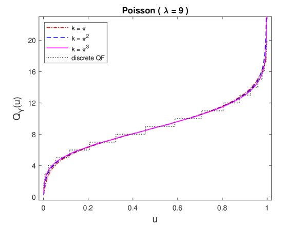
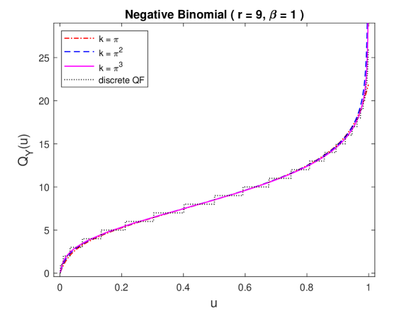
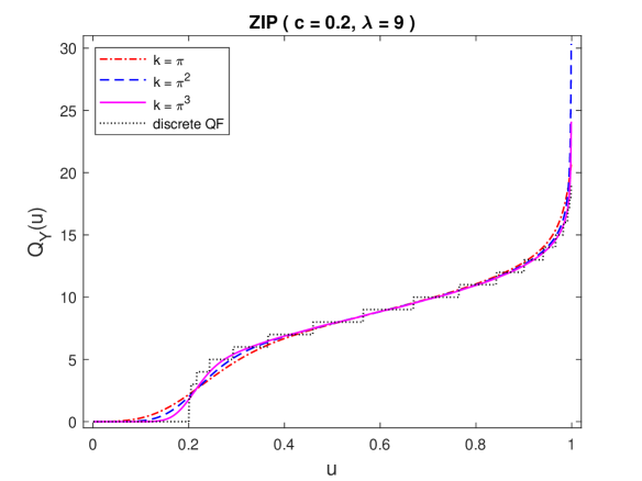
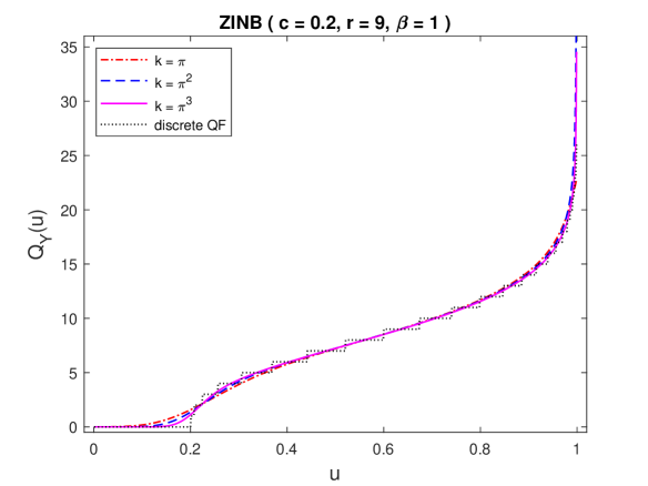
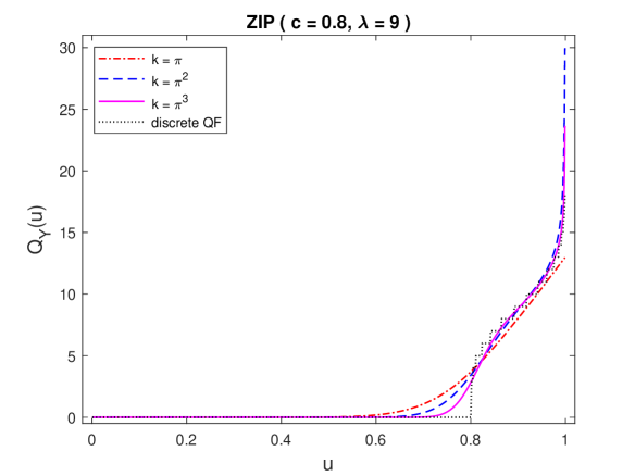
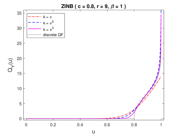
Figure 2.1: Discrete (dotted) and smooth quantile functions of the Poisson (top left), NB (top right), and the corresponding zero-inflated distributions for data truncation intervals $\mu_{Y}\pm k\sigma_{Y}$.

we have depicted the smooth quantile functions $Q^{(k)}_{Y}(u)$ and the discrete quantile functions of Poisson($\lambda=9$) and NB($r=9,\beta=1$) distributions and their zero-inflated versions with $c=0.2$ and $0.8$. The parameters $\lambda$, $r$, and $\beta$ have been selected so that both distributions would have the same mean, but the variance of NB would be two times larger. (For specific parametrization of these distributions, we refer to Klugman et al. (2012).) The smooth curves are constructed using data truncation intervals $\mu_{Y}\pm k\sigma_{Y}$ with $k=\pi,\pi^{2},\pi^{3}$. As we see from the figure, all the three choices of $k$ work well for standard Poisson and NB distributions. However, for their zero-inflated versions ZIP and ZINB the case $k=\pi$ misses both tails of the distribution and $k=\pi^{2}$ can be markedly improved by $k=\pi^{3}$ at the jumps from 0 to 1, 2, 3, or 4. Since typical claim count data contain about 80% of zeros (i.e., $c=0.8$), we recommend using $k$ of the magnitude $\pi^{3}\approx 31$.

2.3 Theoretical Foundations

With $Q^{(k)}_{*}(u)$ and $\widehat{Q}^{(k)}_{*}(u)$ defined by equations (2.12) and (2.13), respectively, the vector

$$\Big{(}Q^{(k)}_{*}(u_{1}),\ldots,Q^{(k)}_{*}(u_{l})\Big{)}$$ (2.15)

of smoothed population quantiles ($0<u_{1}<\cdots<u_{l}<1$) can be estimated by the vector

$$\left(\widehat{Q}^{(k)}_{*}(u_{1}),\ldots,\widehat{Q}^{(k)}_{*}(u_{l})\right)$$ (2.16)

of smoothed sample quantiles. According to our next theorem, the latter vector is a consistent and (jointly) asymptotically normal estimator of vector (2.15).

Theorem 2.1.

Given an i.i.d. sample of size $n$ from a discrete distribution $F_{Y}$ with infinite support $y_{1:d}<y_{2:d}<y_{3:d}<\cdots$ and $d=\infty$, let its truncated version $y_{1:d_{k}}<y_{2:d_{k}}<\cdots<y_{d_{k}:d_{k}}$ with $d_{k}<\infty$ be constructed using the three-part design of Section 2.2. Then, when $n\rightarrow\infty$,

1. $\left(\widehat{Q}^{(k)}_{*}(u_{1}),\ldots,\widehat{Q}^{(k)}_{*}(u_{l})\right)~{}\stackrel{{\scriptstyle\tiny\mathbf{P}}}{{\longrightarrow}}~{}\Big{(}Q^{(k)}_{*}(u_{1}),\ldots,Q^{(k)}_{*}(u_{l})\Big{)}$,

2. $\displaystyle\left(\widehat{Q}^{(k)}_{*}(u_{1}),\ldots,\widehat{Q}^{(k)}_{*}(u_{l})\right)~{}\sim~{}\mathcal{AN}\left(\big{(}Q^{(k)}_{*}(u_{1}),\ldots,Q^{(k)}_{*}(u_{l})\big{)},\,\frac{1}{n}\,\mathbf{HDH^{\prime}}\right)$,

where $\mathbf{D}:=\big{[}d_{ij}\big{]}_{(d_{k}-1)\times(d_{k}-1)}$ with $d_{ij}=d_{ji}=F^{*}_{i(k)}(1-F^{*}_{j(k)})$, $i(k)\leq j(k)$, and $\mathbf{H}:=\big{[}h_{ij}\big{]}_{l\times(d_{k}-1)}$ with $h_{ij}=(y_{j:d_{k}}-y_{j+1:d_{k}})\,b_{\alpha_{u_{i}},\beta_{u_{i}}}(F^{*}_{j(k)})$. Here $b_{\alpha_{u_{i}},\beta_{u_{i}}}$ is the beta p.d.f. with the parameters $\alpha_{u_{i}}=(d_{k}+1)u_{i}$ and $\beta_{u_{i}}=(d_{k}+1)(1-u_{i})$, and the c.d.f. $F^{*}_{j(k)}$ is defined by formula (2.10).

Proof.

Replacing $\widehat{L}_{k}$ and $\widehat{U}_{k}$ in equation (2.9) by $L_{k}$ and $U_{k}$, respectively, which are known constants, we arrive at equation (2.8). Similarly modified equation (2.11) becomes $\widetilde{F}^{*}_{j(k)}=\frac{\widehat{F}_{j(k)}-\widehat{F}_{Y}(L_{k})}{\widehat{F}_{Y}(U_{k})-\widehat{F}_{Y}(L_{k})},$ resulting in the modification

$$\widetilde{Q}^{(k)}_{*}(u)~{}=~{}\sum_{j=1}^{d_{k}}\Big{(}B_{\alpha_{u},\beta_{u}}(\widetilde{F}^{*}_{j(k)})-B_{\alpha_{u},\beta_{u}}(\widetilde{F}^{*}_{j(k)-1})\Big{)}y_{j:d_{k}}$$

of estimator (2.16). This creates the finite domain scenario of Section 2.1. Therefore, the vector estimator

$$\left(\widetilde{Q}^{(k)}_{*}(u_{1}),\ldots,\widetilde{Q}^{(k)}_{*}(u_{l})\right)$$

satisfies statements (i) and (ii). This can be established by following the proof of Brazauskas and Ratnam (2023+, Theorem 3.1). Note first that $\big{(}\overline{Y},S^{2}\big{)}\stackrel{{\scriptstyle\tiny\mathbf{P}}}{{\longrightarrow}}\big{(}\mu_{Y},\sigma_{Y}^{2}\big{)}$ implies $\big{(}\widehat{L}_{k},\widehat{U}_{k}\big{)}\stackrel{{\scriptstyle\tiny\mathbf{P}}}{{\longrightarrow}}\big{(}L_{k},U_{k}\big{)}$, and since by design both $L_{k}\in(y_{1:d_{k}}-1;y_{1:d_{k}})$ and $U_{k}\in(y_{d_{k}:d_{k}};y_{d_{k}:d_{k}}+1)$ are the points where the c.d.f.’s $\widetilde{F}^{*}_{j(k)}$ and $F^{*}_{j(k)}$ are continuous, $\widehat{F}^{*}_{j(k)}\stackrel{{\scriptstyle\tiny\mathbf{P}}}{{\longrightarrow}}F^{*}_{j(k)}$. Now note that $\big{(}\widehat{Q}^{(k)}_{*}(u_{1}),\ldots,\widehat{Q}^{(k)}_{*}(u_{l})\big{)}$ is a continuous transformation of $\widehat{F}^{*}_{1:d_{k}},\ldots,\widehat{F}^{*}_{d_{k}:d_{k}}$. Therefore, an application of the continuous mapping theorem (e.g., Serfling, 1980, Section 1.7) implies

$$\left(\widehat{Q}_{*}^{(k)}(u_{1}),\ldots,\widehat{Q}_{*}^{(k)}(u_{l})\right)\stackrel{{\scriptstyle\tiny\mathbf{P}}}{{\longrightarrow}}\Big{(}Q_{*}^{(k)}(u_{1}),\ldots,Q_{*}^{(k)}(u_{l})\Big{)},$$

which proves part (i) of the theorem.

To prove part (ii), we note the already established result

$$\left(\widetilde{Q}^{(k)}_{*}(u_{1}),\ldots,\widetilde{Q}^{(k)}_{*}(u_{l})\right)~{}\sim~{}\mathcal{AN}\left(\big{(}Q^{(k)}_{*}(u_{1}),\ldots,Q^{(k)}_{*}(u_{l})\big{)},\,\frac{1}{n}\,\mathbf{HDH^{\prime}}\right).$$

Since $\widehat{Q}^{(k)}_{*}(u)$ is $\widetilde{Q}^{(k)}_{*}(u)$ with $(L_{k},U_{k})$ replaced by its consistent estimator $\big{(}\widehat{L}_{k},\widehat{U}_{k}\big{)}$, the generalized Slutsky’s theorem (Demidenko, 2004, Section 13.1.2) assures that estimators $\big{(}\widetilde{Q}^{(k)}_{*}(u_{1}),\ldots,\widetilde{Q}^{(k)}_{*}(u_{l})\big{)}$ and $\big{(}\widehat{Q}^{(k)}_{*}(u_{1}),\ldots,\widehat{Q}^{(k)}_{*}(u_{l})\big{)}$ have the same asymptotic normal distribution. This concludes the proof of part (ii) and establishes Theorem 2.1. ∎

3 Simulated Data Examples

In this section, we conduct a Monte Carlo simulation study with the objective of illustrating the theoretical properties established in Theorem 2.1. We start by describing the study design (Section 3.1) and then provide summarizing tables and associated with them discussions for Poisson and NB distributions (Section 3.2) as well as for their zero-inflated versions ZIP and ZINB (Section 3.3).

3.1 Study Design

The study design is based on the following choices.

1.                                                                                                                                    

2. Simulation Design

3.                                                                                                                                    

   • Discrete distributions.  Poisson$(\lambda=9)$ and negative binomial NB$(r=9,\,\beta=1)$.

   • Zero-inflated discrete distributions.  Zero-inflated Poisson, ZIP$(\lambda=1,\,c=0.8)$, and zero-inflated negative binomial ZINB$(r=1,\,\beta=1,\,c=0.8)$.

   • Key formulas and parameters (for generating data and computing theoretical targets).

     • Means: $\lambda=9$ (Poisson),  $r\beta=9$ (NB),  $\frac{\lambda(1-c)}{1-e^{-\lambda}}=0.32$ (ZIP), and $\frac{r\beta(1-c)}{1-(1+\beta)^{-r}}=0.40$ (ZINB).

     • Variances:  $\lambda=9$ (Poisson),  $r\beta(1+\beta)=18$ (NB), $\frac{1-c}{1-e^{-\lambda}}\left(\lambda+\frac{\lambda^{2}(c-e^{-\lambda})}{1-e^{-\lambda}}\right)=0.53$ (ZIP), and $\frac{1-c}{1-(1+\beta)^{-r}}\left(r\beta(1+\beta)+\frac{(r\beta)^{2}(c-(1+\beta)^{-r})}{1-(1+\beta)^{-r}}\right)=1.04$ (ZINB).

     • Regular proportions of zeros:  $p_{0}=e^{-\lambda}=0.0001$ (Poisson),  $p_{0}=(1+\beta)^{-r}=0.002$ (NB), $\frac{p_{0}(1-c)}{1-p_{0}}=\frac{e^{-\lambda}(1-c)}{1-e^{-\lambda}}=0.12$ (ZIP), and $\frac{p_{0}(1-c)}{1-p_{0}}=\frac{(1+\beta)^{-r}(1-c)}{1-(1+\beta)^{-r}}=0.2$ (ZINB).

     • Excess proportions of zeros:  $0$ (Poisson), $0$ (NB), $\frac{c-p_{0}}{1-p_{0}}=\frac{c-e^{-\lambda}}{1-e^{-\lambda}}=0.68$ (ZIP),
       and $\frac{c-p_{0}}{1-p_{0}}=\frac{c-(1+\beta)^{-r}}{1-(1+\beta)^{-r}}=0.6$ (ZINB).

   • Truncation intervals.  $\overline{Y}\pm k\,S$ for simulated data and $\mu_{Y}\pm k\sigma_{Y}$ for theoretical targets with $k=\pi,\,\pi^{2},\,\pi^{3}$.

   • Sample sizes.  $n=10^{2},\,10^{3},\,10^{4}$.

4.                                                                                                                                    

For any given distribution, we generate 10,000 random samples of a specified length $n$. For each sample, we estimate the quartiles $\big{(}Q_{*}(0.25),Q_{*}(0.50),Q_{*}(0.75)\big{)}$ of the distribution using formula (2.13). We then compute the means and covariance-variance ($\times n$) matrices for the 10,000 estimates of the quartiles. Note that generation of the zero-inflated data requires a two-step procedure. In the first step, the excess portion of zeros is generated from either zero or non-zero values, with the probability of zero being  $\frac{c-p_{0}}{1-p_{0}}$. In the second step, the corresponding regular Poisson or NB distribution is used to generate the remaining portion of zeros (as well all other positive integer values), the probability of which is now equal to  $\frac{p_{0}(1-c)}{1-p_{0}}$. The above two proportions of zeros sum up to $c$, the total proportion of zeros in the sample.

3.2 Poisson and NB Distributions

The parameters of the Poisson and NB distributions are selected to match the models plotted in Figure 2.1. Both distributions have the same mean, but the variance of NB is twice the variance of Poisson. We notice from Table 3.1

Table 3.1: Estimated means and covariance-variance ($\times n$) matrices of the smoothed quartile estimators $\widehat{Q}^{(k)}_{*}(0.25)$, $\widehat{Q}^{(k)}_{*}(0.50)$, $\widehat{Q}^{(k)}_{*}(0.75)$ for the Poisson$(\lambda=9)$ and NB$(r=9,\,\beta=1)$ distributions truncated at the points $\overline{Y}\pm k\,S$ with $k=\pi,\,\pi^{2},\,\pi^{3}$.

	$n=10^{2}$	$n=10^{3}$	$n=10^{4}$	$n=\infty$
Poisson$\,(\lambda=9$), $k=\pi$
$\widehat{means}$	(6.82, 8.84, 11.02)	(6.82, 8.84, 11.02)	(6.82, 8.84, 11.02)	(6.815, 8.835, 11.021)
$\widehat{\textbf{HDH'}}$	$\begin{bmatrix}11.24&8.51&5.91\\ 8.51&11.63&10.10\\ 5.91&10.10&16.00\end{bmatrix}$	$\begin{bmatrix}11.64&8.65&5.78\\ 8.65&11.79&10.20\\ 5.78&10.20&16.29\end{bmatrix}$	$\begin{bmatrix}11.42&8.39&5.54\\ 8.39&11.45&9.67\\ 5.54&9.67&15.45\end{bmatrix}$	$\begin{bmatrix}11.367&8.360&5.539\\ 8.360&11.497&9.753\\ 5.539&9.753&15.478\end{bmatrix}$
Poisson$\,(\lambda=9)$, $k=\pi^{2}$
$\widehat{means}$	(6.86, 8.84, 10.98)	(6.86, 8.84, 10.98)	(6.86, 8.84, 10.98)	(6.856, 8.838, 10.982)
$\widehat{\textbf{HDH'}}$	$\begin{bmatrix}12.05&8.38&5.71\\ 8.38&12.28&9.73\\ 5.71&9.73&16.52\end{bmatrix}$	$\begin{bmatrix}12.42&8.58&5.69\\ 8.58&12.45&9.95\\ 5.69&9.95&17.00\end{bmatrix}$	$\begin{bmatrix}12.20&8.34&5.57\\ 8.34&12.23&9.62\\ 5.57&9.62&16.51\end{bmatrix}$	$\begin{bmatrix}12.153&8.309&5.526\\ 8.309&12.289&9.714\\ 5.526&9.714&16.579\end{bmatrix}$
Poisson$\,(\lambda=9)$, $k=\pi^{3}$
$\widehat{means}$	(6.89, 8.84, 10.94)	(6.89, 8.85, 10.95)	(6.89, 8.85, 10.95)	(6.893, 8.853, 10.951)
$\widehat{\textbf{HDH'}}$	$\begin{bmatrix}12.90&8.20&5.61\\ 8.20&13.17&9.55\\ 5.61&9.55&17.79\end{bmatrix}$	$\begin{bmatrix}11.32&7.55&5.08\\ 7.55&12.00&9.01\\ 5.08&9.01&16.91\end{bmatrix}$	$\begin{bmatrix}10.61&7.09&4.83\\ 7.09&11.45&8.49\\ 4.83&8.49&15.77\end{bmatrix}$	$\begin{bmatrix}10.533&7.033&4.695\\ 7.033&11.401&8.415\\ 4.695&8.415&15.631\end{bmatrix}$
NB$\,(r=9,\,\beta=1)$, $k=\pi$
$\widehat{means}$	(5.88, 8.51, 11.64)	(5.86, 8.50, 11.63)	(5.86, 8.50, 11.63)	(5.859, 8.504, 11.628)
$\widehat{\textbf{HDH'}}$	$\begin{bmatrix}18.66&15.35&11.46\\ 15.35&23.08&21.45\\ 11.46&21.45&36.85\end{bmatrix}$	$\begin{bmatrix}18.48&15.12&11.22\\ 15.12&23.17&21.48\\ 11.22&21.48&37.13\end{bmatrix}$	$\begin{bmatrix}18.10&14.53&10.21\\ 14.53&22.35&20.27\\ 10.21&20.27&35.13\end{bmatrix}$	$\begin{bmatrix}18.038&14.458&10.384\\ 14.458&22.085&20.054\\ 10.384&20.054&34.815\end{bmatrix}$
NB$\,(r=9,\,\beta=1)$, $k=\pi^{2}$
$\widehat{means}$	(5.92, 8.52, 11.61)	(5.90, 8.52, 11.61)	(5.90, 8.52, 11.60)	(5.904, 8.515, 11.604)
$\widehat{\textbf{HDH'}}$	$\begin{bmatrix}20.08&15.10&11.04\\ 15.10&24.18&20.33\\ 11.04&20.33&37.06\end{bmatrix}$	$\begin{bmatrix}19.84&14.90&10.84\\ 14.90&24.36&20.41\\ 10.84&20.41&37.45\end{bmatrix}$	$\begin{bmatrix}19.51&14.46&10.25\\ 14.46&23.91&20.10\\ 10.25&20.10&37.35\end{bmatrix}$	$\begin{bmatrix}19.552&14.467&10.507\\ 14.467&23.833&20.212\\ 10.507&20.212&37.975\end{bmatrix}$
NB$\,(r=9,\,\beta=1)$, $k=\pi^{3}$
$\widehat{means}$	(5.93, 8.51, 11.56)	(5.93, 8.51, 11.56)	(5.93, 8.50, 11.55)	(5.928, 8.504, 11.554)
$\widehat{\textbf{HDH'}}$	$\begin{bmatrix}21.65&14.95&10.99\\ 14.95&25.66&20.11\\ 10.99&20.11&39.37\end{bmatrix}$	$\begin{bmatrix}19.16&14.41&10.20\\ 14.41&27.72&20.75\\ 10.20&20.75&40.10\end{bmatrix}$	$\begin{bmatrix}17.74&13.80&9.44\\ 13.80&28.35&20.84\\ 9.44&20.84&40.31\end{bmatrix}$	$\begin{bmatrix}17.673&13.777&9.675\\ 13.777&28.408&20.920\\ 9.675&20.920&40.813\end{bmatrix}$
Note:  The entries for $n<\infty$ are the averages and sample covariances of estimated quartiles.
Results are based on 10,000 simulated samples. Standard errors of these entries are $\leq 0.01$.

a rapid convergence of the estimated means and covariance-variance ($\times n$) matrices of smoothed quartile estimators. Even the entries for $n=100$ are close to their respective theoretical targets, which are reported in the column $n=\infty$. Furthermore, as it could be anticipated from Figure 2.1, the choice of $k$ for these distributions is not essential. We recommend choosing $k=\pi^{2}$ as sufficient for most typical discrete distributions (no zero inflated cases though). Finally, note that the estimated means of the estimators look similar for Poisson and NB distributions while the entries of the covariance-variance matrices differ by a factor of (roughly) two. This is expected, and it is due to the choice of parameters of the Poisson and NB distributions.

3.3 ZIP and ZINB Distributions

The parameters of the ZIP and ZINB distributions are selected to match the models depicted in Figure 2.1 (third column). The choices of $\lambda=r\beta=1$ and $c=0.8$ represent realistic insurance data scenarios. We notice from Table 3.2

Table 3.2: Estimated means and covariance-variance ($\times n$) matrices of the smoothed quartile estimators $\widehat{Q}^{(k)}_{*}(0.25)$, $\widehat{Q}^{(k)}_{*}(0.50)$, $\widehat{Q}^{(k)}_{*}(0.75)$ for the ZIP$(\lambda=1,\,c=0.8)$ and ZINB$(r=1,\,\beta=1,\,c=0.8)$ distributions truncated at the points $\overline{Y}\pm k\,S$ with $k=\pi,\,\pi^{2},\,\pi^{3}$.

	$n=10^{2}$	$n=10^{3}$	$n=10^{4}$	$n=\infty$
ZIP$\,(\lambda=1,\,c=0.8$), $k=\pi$
$\widehat{means}$	(0.01, 0.10, 0.62)	(0.01, 0.10, 0.62)	(0.01, 0.10, 0.62)	(0.006, 0.095, 0.616)
$\widehat{\textbf{HDH'}}$	$\begin{bmatrix}0.00&0.02&0.06\\ 0.02&0.23&0.80\\ 0.06&0.80&3.80\end{bmatrix}$	$\begin{bmatrix}0.00&0.02&0.06\\ 0.02&0.22&0.69\\ 0.06&0.69&2.50\end{bmatrix}$	$\begin{bmatrix}0.00&0.02&0.06\\ 0.02&0.21&0.66\\ 0.06&0.66&2.23\end{bmatrix}$	$\begin{bmatrix}0.001&0.015&0.044\\ 0.015&0.150&0.461\\ 0.044&0.461&1.522\end{bmatrix}$
ZIP$\,(\lambda=1,\,c=0.8$), $k=\pi^{2}$
$\widehat{means}$	(0.00, 0.03, 0.53)	(0.00, 0.03, 0.52)	(0.00, 0.03, 0.51)	(0.000, 0.026, 0.514)
$\widehat{\textbf{HDH'}}$	$\begin{bmatrix}0.00&0.00&0.00\\ 0.00&0.06&0.31\\ 0.00&0.31&2.63\end{bmatrix}$	$\begin{bmatrix}0.00&0.00&0.00\\ 0.00&0.05&0.31\\ 0.00&0.31&2.88\end{bmatrix}$	$\begin{bmatrix}0.00&0.00&0.01\\ 0.00&0.05&0.41\\ 0.01&0.41&3.60\end{bmatrix}$	$\begin{bmatrix}0.000&0.000&0.004\\ 0.000&0.041&0.318\\ 0.004&0.318&2.709\end{bmatrix}$
ZIP$\,(\lambda=1,\,c=0.8$), $k=\pi^{3}$
$\widehat{means}$	(0.00, 0.00, 0.35)	(0.00, 0.00, 0.32)	(0.00, 0.00, 0.31)	(0.000, 0.001, 0.315)
$\widehat{\textbf{HDH'}}$	$\begin{bmatrix}0.00&0.00&0.00\\ 0.00&0.00&0.06\\ 0.00&0.06&3.65\end{bmatrix}$	$\begin{bmatrix}0.00&0.00&0.00\\ 0.00&0.00&0.02\\ 0.00&0.02&4.07\end{bmatrix}$	$\begin{bmatrix}0.00&0.00&0.00\\ 0.00&0.00&0.02\\ 0.00&0.02&3.94\end{bmatrix}$	$\begin{bmatrix}0.000&0.000&0.000\\ 0.000&0.000&0.021\\ 0.000&0.021&3.400\end{bmatrix}$
ZINB$\,(r=1,\,\beta=1,\,c=0.8$), $k=\pi$
$\widehat{means}$	(0.00, 0.08, 0.64)	(0.00, 0.07, 0.65)	(0.00, 0.07, 0.64)	(0.003, 0.069, 0.642)
$\widehat{\textbf{HDH'}}$	$\begin{bmatrix}0.00&0.01&0.04\\ 0.01&0.19&0.79\\ 0.04&0.79&4.87\end{bmatrix}$	$\begin{bmatrix}0.00&0.01&0.03\\ 0.01&0.18&0.72\\ 0.03&0.72&4.40\end{bmatrix}$	$\begin{bmatrix}0.00&0.01&0.04\\ 0.01&0.17&0.75\\ 0.04&0.75&3.76\end{bmatrix}$	$\begin{bmatrix}0.000&0.007&0.029\\ 0.007&0.119&0.519\\ 0.029&0.519&2.534\end{bmatrix}$
ZINB$\,(r=1,\,\beta=1,\,c=0.8$), $k=\pi^{2}$
$\widehat{means}$	(0.00, 0.02, 0.53)	(0.00, 0.01, 0.50)	(0.00, 0.01, 0.49)	(0.000, 0.012, 0.489)
$\widehat{\textbf{HDH'}}$	$\begin{bmatrix}0.00&0.00&0.00\\ 0.00&0.04&0.28\\ 0.00&0.28&3.96\end{bmatrix}$	$\begin{bmatrix}0.00&0.00&0.00\\ 0.00&0.02&0.24\\ 0.00&0.24&4.25\end{bmatrix}$	$\begin{bmatrix}0.00&0.00&0.00\\ 0.00&0.02&0.29\\ 0.00&0.29&4.74\end{bmatrix}$	$\begin{bmatrix}0.000&0.000&0.001\\ 0.000&0.014&0.223\\ 0.001&0.223&3.781\end{bmatrix}$
ZINB$\,(r=1,\,\beta=1,\,c=0.8$), $k=\pi^{3}$
$\widehat{means}$	(0.00, 0.00, 0.33)	(0.00, 0.00, 0.28)	(0.00, 0.00, 0.27)	(0.000, 0.000, 0.270)
$\widehat{\textbf{HDH'}}$	$\begin{bmatrix}0.00&0.00&0.00\\ 0.00&0.00&0.03\\ 0.00&0.03&4.83\end{bmatrix}$	$\begin{bmatrix}0.00&0.00&0.00\\ 0.00&0.00&0.01\\ 0.00&0.01&5.22\end{bmatrix}$	$\begin{bmatrix}0.00&0.00&0.00\\ 0.00&0.00&0.00\\ 0.00&0.00&5.11\end{bmatrix}$	$\begin{bmatrix}0.000&0.000&0.000\\ 0.000&0.000&0.003\\ 0.000&0.003&4.155\end{bmatrix}$
Note:  The entries for $n<\infty$ are the averages and sample covariances of estimated quartiles.
Results are based on 10,000 simulated samples. Standard errors of these entries are $\leq 0.01$.

that convergence of the estimated means and covariance-variance ($\times n$) matrices of smoothed quartile estimators is not as fast as that of the Poisson and NB distributions. It also depends on the width of the truncation interval. While the choice of $k=\pi^{2}$ yields reasonable results, $k=\pi^{3}$ offers an improvement. This observation agrees with the recommendation based on Figure 2.1. In addition, note that the estimated means of all quartile estimators are shrinking toward zero. This is supposed to happen because all three quartile levels are below $c=0.8$. Naturally, the mean estimates that are close to zero result in similar values (almost 0) of the covariance-variance estimates.

4 Bootstrap Approximation

Using simulations in Section 3, we have illustrated the statements of Theorem 2.1. In the current section, we shall further harness the power of computers and construct a bootstrap algorithm that will help us to approximate the results of Section 2. Note that if properly designed, bootstrap procedures can be used to approximate even more challenging risk measurement tasks than smoothing of discrete quantiles. In Section 4.1, the algorithm for bootstrap estimation is outlined. In Section 4.2, the performance of the algorithm is validated and cross-checked with Theorem 2.1 for the Poisson, NB, ZIP, and ZINB distributions.

4.1 The Algorithm

The bootstrap algorithm requires specifications of the following inputs:

• Data is a sample generated by some distribution

• $n$ is the sample size

• $m$ is the number of bootstrapped resamples

• $k$ is the number of standard deviations in interval (2.3)

• $u_{1},\ldots,u_{l}$ are the quantile levels of vectors (2.15) and (2.16)

In the description of the algorithm, we use $\boldsymbol{y}$ to denote resampled data, whose sample mean and the sample standard deviation we denote by $\overline{\boldsymbol{y}}$ and $s_{\boldsymbol{y}}$, respectively. Furthermore, given any $y\in\boldsymbol{y}$, we use the notation $\mbox{freq}(y)$ for the number of $y$’s in the data set $\boldsymbol{y}$.

1.                                                                                                                                    

2. Algorithm for Bootstrap Approximation

3.                                                                                                                                    

4. Input  Data;  $n$;  $m$;  $k$;  $u_{1},\ldots,u_{l}$

5. for  $i=1,\ldots,m$  do

   1. ResampledData $(=:\boldsymbol{y})$ = bootstrap(Data, with Replacement)

   2. $\widehat{L}_{k}$ = max($-0.5,\,\overline{\boldsymbol{y}}-ks_{\boldsymbol{y}}$),  $\widehat{U}_{k}=\overline{\boldsymbol{y}}+ks_{\boldsymbol{y}}$

   3. $\widehat{y}_{1:\widehat{d}_{k}}$ = ceiling($\widehat{L}_{k}$),  $\widehat{y}_{\widehat{d}_{k}:\widehat{d}_{k}}$ = floor($\widehat{U}_{k}$) / see (2.9) /

   4. $\widehat{d}_{k}=\widehat{y}_{\widehat{d}_{k}:\widehat{d}_{k}}-\widehat{y}_{1:\widehat{d}_{k}}+1$,  $\widehat{y}_{j:\widehat{d}_{k}}=\widehat{y}_{1:\widehat{d}_{k}}+j-1$

   5. for  $j=1,\ldots,\widehat{d}_{k}$  do

      1. $\widehat{F}_{j(k)}$ = $\left(\mbox{freq}(\widehat{y}_{1:\widehat{d}_{k}})+\cdots+\mbox{freq}(\widehat{y}_{j:\widehat{d}_{k}})\right)\Big{/}n$

   6. end for

   7. $\widehat{F}_{Y}(\widehat{L}_{k})=\left(\mbox{freq}\big{(}y\in\boldsymbol{y}\mbox{ such that }y<\widehat{y}_{1:\widehat{d}_{k}}\big{)}\right)\Big{/}n$

   8. $\widehat{F}_{Y}(\widehat{U}_{k})=\widehat{F}_{Y}(\widehat{L}_{k})+\left(\mbox{freq}(\widehat{y}_{1:\widehat{d}_{k}})+\cdots+\mbox{freq}(\widehat{y}_{\widehat{d}_{k}:\widehat{d}_{k}})\right)\Big{/}n$

   9. $\widehat{F}_{j(k)}^{\ast}=\left(\widehat{F}_{j(k)}-\widehat{F}_{Y}(\widehat{L}_{k})\right)\Big{/}\left(\widehat{F}_{Y}(\widehat{U}_{k})-\widehat{F}_{Y}(\widehat{L}_{k})\right)$ / see (2.11) /

   10. for  $u=u_{1},\ldots,u_{l}$  do

       1. $\widehat{\alpha}_{u}=(\widehat{d}_{k}+1)u$,  $\widehat{\beta}_{u}=(\widehat{d}_{k}+1)(1-u)$

       2. $\widehat{Q}^{(k)}_{*}(u)=\sum_{j=1}^{\widehat{d}_{k}}\Big{(}B_{\widehat{\alpha}_{u},\widehat{\beta}_{u}}(\widehat{F}^{*}_{j(k)})-B_{\widehat{\alpha}_{u},\widehat{\beta}_{u}}(\widehat{F}^{*}_{j(k)-1})\Big{)}\widehat{y}_{j:\widehat{d}_{k}}$ / see (2.13) /

   11. end for

   12. Store $\widehat{Q}^{(k)}_{*}(u)$ in $m\times l$ matrix

6. end for

7. $\mbox{\bf{column Means}}(\bf{\widehat{Q}^{(k)}_{*}(u))}$ = colMeans($m\times l$ matrix)

8. $\bf{\widehat{\Sigma}(\widehat{Q}^{(k)}_{*}(u))}$ = cov($m\times l$ matrix)

9.                                                                                                                                    

4.2 Validation of the Algorithm

According to the bootstrap algorithm of Section 4.1, and given a sample of size $n$ from some distribution, the sample is empirically resampled with replacement (bootstrapped) and the smoothed quartile estimates are computed. This cycle is repeated 10,000 times. The means and covariance-variance matrices of the 10,000 estimates are then computed and summarized. The results are reported in Tables 4.1–4.2.

Table 4.1: Bootstrapped means and covariance-variance ($\times n$) matrices of the smoothed quartile estimators $\widehat{Q}^{(k)}_{*}(0.25)$, $\widehat{Q}^{(k)}_{*}(0.50)$, $\widehat{Q}^{(k)}_{*}(0.75)$ for the Poisson$(\lambda=9)$ and NB$(r=9,\,\beta=1)$ distributions truncated at the points $\overline{y}\pm k\,s$ with $k=\pi,\,\pi^{2},\,\pi^{3}$.

	$n=10^{2}$	$n=10^{3}$	$n=10^{4}$	$n=\infty$
Poisson$\,(\lambda=9)$, $k=\pi$
$\widehat{means}$	(7.29, 9.06, 10.98)	(6.87, 8.80, 11.05)	(6.81, 8.82, 11.08)	(6.815, 8.835, 11.021)
$\widehat{\textbf{HDH'}}$	$\begin{bmatrix}9.51&6.90&3.79\\ 6.90&10.49&7.26\\ 3.79&7.26&8.46\end{bmatrix}$	$\begin{bmatrix}11.13&7.73&5.58\\ 7.73&10.89&9.80\\ 5.58&9.80&16.04\end{bmatrix}$	$\begin{bmatrix}11.95&8.58&5.84\\ 8.58&11.92&10.45\\ 5.84&10.45&16.46\end{bmatrix}$	$\begin{bmatrix}11.367&8.360&5.539\\ 8.360&11.497&9.753\\ 5.539&9.753&15.478\end{bmatrix}$
Poisson$\,(\lambda=9)$, $k=\pi^{2}$
$\widehat{means}$	(7.37, 9.03, 10.95)	(6.91, 8.78, 11.01)	(6.86, 8.81, 11.04)	(6.856, 8.838, 10.982)
$\widehat{\textbf{HDH'}}$	$\begin{bmatrix}10.63&7.32&3.44\\ 7.32&12.75&7.08\\ 3.44&7.08&7.83\end{bmatrix}$	$\begin{bmatrix}13.30&8.28&5.71\\ 8.28&12.09&9.52\\ 5.71&9.52&15.87\end{bmatrix}$	$\begin{bmatrix}12.83&8.59&5.88\\ 8.59&12.80&10.45\\ 5.88&10.45&17.71\end{bmatrix}$	$\begin{bmatrix}12.153&8.309&5.526\\ 8.309&12.289&9.714\\ 5.526&9.714&16.579\end{bmatrix}$
Poisson$\,(\lambda=9)$, $k=\pi^{3}$
$\widehat{means}$	(7.44, 9.01, 10.95)	(6.93, 8.77, 10.97)	(6.89, 8.82, 11.00)	(6.893, 8.853, 10.951)
$\widehat{\textbf{HDH'}}$	$\begin{bmatrix}12.76&8.25&3.15\\ 8.25&15.14&6.36\\ 3.15&6.36&6.71\end{bmatrix}$	$\begin{bmatrix}14.63&9.08&5.25\\ 9.08&14.10&8.54\\ 5.25&8.54&13.40\end{bmatrix}$	$\begin{bmatrix}11.29&7.72&5.11\\ 7.72&13.10&9.55\\ 5.11&9.55&17.36\end{bmatrix}$	$\begin{bmatrix}10.533&7.033&4.695\\ 7.033&11.401&8.415\\ 4.695&8.415&15.631\end{bmatrix}$
NB$\,(r=9,\,\beta=1)$, $k=\pi$
$\widehat{means}$	(5.68, 8.08, 10.42)	(5.84, 8.40, 11.78)	(5.82, 8.44, 11.58)	(5.859, 8.504, 11.628)
$\widehat{\textbf{HDH'}}$	$\begin{bmatrix}17.82&11.60&8.80\\ 11.60&13.45&12.47\\ 8.80&12.47&25.04\end{bmatrix}$	$\begin{bmatrix}17.14&13.94&12.20\\ 13.94&21.49&23.88\\ 12.20&23.88&48.24\end{bmatrix}$	$\begin{bmatrix}17.21&13.97&10.42\\ 13.97&21.70&20.33\\ 10.42&20.33&35.85\end{bmatrix}$	$\begin{bmatrix}18.038&14.458&10.384\\ 14.458&22.085&20.054\\ 10.384&20.054&34.815\end{bmatrix}$
NB$\,(r=9,\,\beta=1)$, $k=\pi^{2}$
$\widehat{means}$	(5.74, 8.11, 10.25)	(5.89, 8.38, 11.72)	(5.87, 8.44, 11.55)	(5.904, 8.515, 11.604)
$\widehat{\textbf{HDH'}}$	$\begin{bmatrix}18.13&10.75&8.17\\ 10.75&13.65&11.62\\ 8.17&11.62&24.02\end{bmatrix}$	$\begin{bmatrix}16.26&12.38&11.39\\ 12.38&20.91&22.39\\ 11.39&22.39&51.69\end{bmatrix}$	$\begin{bmatrix}17.84&13.48&10.22\\ 13.48&22.77&19.74\\ 10.22&19.74&37.65\end{bmatrix}$	$\begin{bmatrix}19.552&14.467&10.507\\ 14.467&23.833&20.212\\ 10.507&20.212&37.975\end{bmatrix}$
NB$\,(r=9,\,\beta=1)$, $k=\pi^{3}$
$\widehat{means}$	(5.79, 8.13, 10.13)	(5.93, 8.35, 11.67)	(5.90, 8.42, 11.51)	(5.928, 8.504, 11.554)
$\widehat{\textbf{HDH'}}$	$\begin{bmatrix}16.54&8.81&6.47\\ 8.81&13.06&9.81\\ 6.47&9.81&20.80\end{bmatrix}$	$\begin{bmatrix}11.35&9.61&9.30\\ 9.61&22.65&22.73\\ 9.30&22.73&58.05\end{bmatrix}$	$\begin{bmatrix}15.05&12.05&8.99\\ 12.05&26.48&20.26\\ 8.99&20.26&40.64\end{bmatrix}$	$\begin{bmatrix}17.673&13.777&9.675\\ 13.777&28.408&20.920\\ 9.675&20.920&40.813\end{bmatrix}$
Note:  The entries for $n<\infty$ are the averages and sample covariances of estimated quartiles.
Results are based on 10,000 bootstrap resamples.

Table 4.2: Bootstrapped means and covariance-variance ($\times n$) matrices of the smoothed quartile estimators $\widehat{Q}^{(k)}_{*}(0.25)$, $\widehat{Q}^{(k)}_{*}(0.50)$, $\widehat{Q}^{(k)}_{*}(0.75)$ for the ZIP$(\lambda=1,\,c=0.8)$ and ZINB$(r=1,\,\beta=1,\,c=0.8)$ distributions truncated at the points $\overline{y}\pm k\,s$ with $k=\pi,\,\pi^{2},\,\pi^{3}$.

	$n=10^{2}$	$n=10^{3}$	$n=10^{4}$	$n=\infty$
ZIP$\,(\lambda=1,\,c=0.8$), $k=\pi$
$\widehat{means}$	(0.00, 0.08, 0.54)	(0.01, 0.09, 0.58)	(0.01, 0.10, 0.62)	(0.006, 0.095, 0.616)
$\widehat{\textbf{HDH'}}$	$\begin{bmatrix}0.00&0.01&0.03\\ 0.01&0.13&0.57\\ 0.03&0.57&3.96\end{bmatrix}$	$\begin{bmatrix}0.00&0.01&0.04\\ 0.01&0.14&0.43\\ 0.04&0.43&1.46\end{bmatrix}$	$\begin{bmatrix}0.00&0.02&0.05\\ 0.02&0.16&0.48\\ 0.05&0.48&1.56\end{bmatrix}$	$\begin{bmatrix}0.001&0.015&0.044\\ 0.015&0.150&0.461\\ 0.044&0.461&1.522\end{bmatrix}$
ZIP$\,(\lambda=1,\,c=0.8$), $k=\pi^{2}$
$\widehat{means}$	(0.00, 0.03, 0.52)	(0.00, 0.03, 0.49)	(0.00, 0.03, 0.52)	(0.000, 0.026, 0.514)
$\widehat{\textbf{HDH'}}$	$\begin{bmatrix}0.00&0.00&0.00\\ 0.00&0.04&0.22\\ 0.00&0.22&2.12\end{bmatrix}$	$\begin{bmatrix}0.00&0.00&0.00\\ 0.00&0.03&0.19\\ 0.00&0.19&1.64\end{bmatrix}$	$\begin{bmatrix}0.00&0.00&0.00\\ 0.00&0.05&0.33\\ 0.00&0.33&2.73\end{bmatrix}$	$\begin{bmatrix}0.000&0.000&0.004\\ 0.000&0.041&0.318\\ 0.004&0.318&2.709\end{bmatrix}$
ZIP$\,(\lambda=1,\,c=0.8$), $k=\pi^{3}$
$\widehat{means}$	(0.00, 0.00, 0.36)	(0.00, 0.00, 0.29)	(0.00, 0.00, 0.33)	(0.000, 0.001, 0.315)
$\widehat{\textbf{HDH'}}$	$\begin{bmatrix}0.00&0.00&0.00\\ 0.00&0.00&0.03\\ 0.00&0.03&3.11\end{bmatrix}$	$\begin{bmatrix}0.00&0.00&0.000\\ 0.00&0.00&0.02\\ 0.00&0.02&2.57\end{bmatrix}$	$\begin{bmatrix}0.00&0.00&0.000\\ 0.00&0.00&0.02\\ 0.00&0.02&3.12\end{bmatrix}$	$\begin{bmatrix}0.000&0.000&0.000\\ 0.000&0.000&0.021\\ 0.000&0.021&3.400\end{bmatrix}$
ZINB$\,(r=1,\,\beta=1,\,c=0.8$), $k=\pi$
$\widehat{means}$	(0.00, 0.06, 0.46)	(0.00, 0.06, 0.58)	(0.00, 0.07, 0.64)	(0.003, 0.069, 0.642)
$\widehat{\textbf{HDH'}}$	$\begin{bmatrix}0.00&0.01&0.02\\ 0.01&0.08&0.32\\ 0.02&0.32&1.72\end{bmatrix}$	$\begin{bmatrix}0.00&0.01&0.02\\ 0.01&0.10&0.42\\ 0.02&0.42&2.49\end{bmatrix}$	$\begin{bmatrix}0.00&0.01&0.03\\ 0.01&0.12&0.53\\ 0.03&0.53&2.62\end{bmatrix}$	$\begin{bmatrix}0.000&0.007&0.029\\ 0.007&0.119&0.519\\ 0.029&0.519&2.534\end{bmatrix}$
ZINB$\,(r=1,\,\beta=1,\,c=0.8$), $k=\pi^{2}$
$\widehat{means}$	(0.00, 0.01, 0.36)	(0.00, 0.01, 0.47)	(0.00, 0.01, 0.48)	(0.000, 0.012, 0.489)
$\widehat{\textbf{HDH'}}$	$\begin{bmatrix}0.00&0.00&0.00\\ 0.00&0.01&0.01\\ 0.00&0.01&1.42\end{bmatrix}$	$\begin{bmatrix}0.00&0.00&0.00\\ 0.00&0.01&0.15\\ 0.00&0.15&2.52\end{bmatrix}$	$\begin{bmatrix}0.00&0.00&0.00\\ 0.00&0.02&0.20\\ 0.00&0.20&3.17\end{bmatrix}$	$\begin{bmatrix}0.000&0.000&0.001\\ 0.000&0.014&0.223\\ 0.001&0.223&3.781\end{bmatrix}$
ZINB$\,(r=1,\,\beta=1,\,c=0.8$), $k=\pi^{3}$
$\widehat{means}$	(0.00, 0.00, 0.17)	(0.00, 0.00, 0.25)	(0.00, 0.00, 0.26)	(0.000, 0.000, 0.270)
$\widehat{\textbf{HDH'}}$	$\begin{bmatrix}0.00&0.00&0.00\\ 0.00&0.00&0.00\\ 0.00&0.00&1.40\end{bmatrix}$	$\begin{bmatrix}0.00&0.00&0.00\\ 0.00&0.00&0.00\\ 0.00&0.00&3.05\end{bmatrix}$	$\begin{bmatrix}0.00&0.00&0.00\\ 0.00&0.00&0.00\\ 0.00&0.00&3.45\end{bmatrix}$	$\begin{bmatrix}0.000&0.000&0.000\\ 0.000&0.000&0.003\\ 0.000&0.003&4.155\end{bmatrix}$
Note:  The entries for $n<\infty$ are the averages and sample covariances of estimated quartiles.
Results are based on 10,000 bootstrap resamples.

As we see from the tables, the bootstrap algorithm approximates the theoretical values established in Theorem 2.1 reasonably well. For the Poisson and NB distributions, $n\geq 100$ with $k=\pi^{2}$ is sufficient in most cases. For the ZIP and ZINB distributions, $n=100$ may be too small, even with $k=\pi^{3}$, but for $n=1000$ and larger sample sizes, the algorithm performs well. Note that to save space in the tables, the entries of the covariance-variance matrices are multiplied by $n$. These numbers then may give the misleading impression that the discrepancies between the bootstrap and theoretical approximations are large, but it can be checked that they are not. For example, in Table 4.1 for $n=100$, Poisson, $k=\pi^{2}$, and the matrix entry $(3,3)$, we actually have $7.83/100=0.0783$ (bootstrap) and $16.579/100=0.1658$ (theoretical). In Table 4.2 for $n=1000$, ZINB, $k=\pi^{3}$, and the matrix entry $(3,3)$, we actually have $3.05/1000=0.0031$ (bootstrap) and $4.155/1000=0.0042$ (theoretical).

5 Real Data Examples

In this section, the newly developed methodology is applied to automobile accident data set (Klugman et al., 2012) and its three modifications. Specifically, in Section 5.1, the data sets are presented and described. In Section 5.2, conditional five number summaries are computed for the four data sets and supplemented with 95% (pointwise) confidence intervals. In Section 5.3, point estimates of a few tail probabilities are evaluated using the traditional discrete probabillity approximation as well as the new smoothed approach.

5.1 Data Sets

The automobile accident data (Klugman et al., 2012, Table 6.2) represent the risk profile of 9,461 insurance policies. Following the numerical examples of Brazauskas and Ratnam (2023+, Section 5.3), we also consider three tail modifications of this data set. Specifically, we take 140 policies (corresponding to about 1.5% of the portfolio) that report 0 accidents and replace them with 140 policies that report at least 2 accidents; this results in three different scenarios. In Table 5.1,

Table 5.1: Original and modified data sets consisting of the numbers of accidents per policy.

Data Set	Number of Accidents									Total Number
	0	1	2	3	4	5	6	7	$\geq 8$	of Policies
O (original)	7,840	1,317	239	42	14	4	4	1	0	9,461
M1 (modified #1)	7,700	1,317	379	42	14	4	4	1	0	9,461
M2 (modified #2)	7,700	1,317	279	62	34	24	24	21	0	9,461
M3 (modified #3)	7,700	1,317	239	42	14	4	4	141	0	9,461

the original and the three modified data sets are provided. The modified counts of policies are italicized.

At first glance, M1, M2, M3 appear to be riskier portfolios than the original data set O. Also noticeable is a progression from the least risky (M1) to the most risky portfolio (M3). The goal of our subsequent computations is to check if these preliminary observations are supported by the new methodology.

5.2 Conditional Five Number Summaries

To illustrate how the joint behavior of smoothed quantiles helps to assess tail riskiness of portfolios, we use the data sets of Table 5.1 and perform C5NS computations. The results are reported in Table 5.2.

Table 5.2: C5NS beyond VaR_0.90 (with 95% confidence intervals in parentheses) for the original and modified automobile data sets.

Data	Summarizing Quantiles (above the VaR0.90 level)
Set	$q_{0.91}$	$q_{0.925}$	$q_{0.95}$	$q_{0.975}$	$q_{0.99}$
O	1.35 $(1.28;\,1.41)$	1.60 $(1.51;\,1.68)$	2.28 $(2.14;\,2.43)$	3.70 $(3.48;\,3.92)$	5.33 $(5.15;\,5.50)$
M1	1.47 $(1.40;\,1.53)$	1.71 $(1.63;\,1.80)$	2.38 $(2.24;\,2.52)$	3.76 $(3.54;\,3.97)$	5.35 $(5.17;\,5.52)$
M2	1.86 $(1.76;\,1.96)$	2.25 $(2.13;\,2.37)$	3.19 $(3.05;\,3.34)$	4.69 $(4.56;\,4.82)$	5.96 $(5.89;\,6.04)$
M3	2.30 $(2.16;\,2.43)$	2.79 $(2.64;\,2.93)$	3.85 $(3.69;\,4.00)$	5.26 $(5.15;\,5.37)$	6.27 $(6.22;\,6.33)$
Note:  Results are based on Theorem 2.1, with the truncation points $\overline{Y}\pm\pi^{3}S$.

We see from the table that the C5NS approach supports the intuitive conclusions about O, M1, M2, and M3 (see Section 5.1). Indeed, as the 140 policies that have 0 accidents in the original data set O report higher numbers of accidents (all of them have 2 accidents in M1 and 7 in M3), the five quantiles used in C5NS gradually and simultaneously increase. Also, the associated confidence intervals are relatively narrow and in general do not overlap (except the intervals for O and M1). This implies that the portfolios could be statistically separated and classified as follows: O is the least risky, M1 is somewhat riskier than O, M2 is significantly riskier than M1, and M3 is the most risky. Of course, for this type of statistical inference the joint asymptotic normality of the quantiles was not used. Such a result would be needed, however, if one decided to combine the quantiles by, for example, taking a weighted average of them.

5.3 Tail Probabilities

To demonstrate the advantages of the smoothed approach over the commonly used linear interpolation (Klugman et al., 2012, Section 13.1), we estimate several tail probabilities and evaluate the standard error and the coefficient of variation (CV) of those estimates. Specifically, for the smoothed variable $Y^{*}$, we compute a tail probability by first inverting the quantile function and then evaluating $\mathbf{P}\{Y^{*}>a^{*}\}$ directly if $a^{*}$ is non-integer or by applying the 0.5 continuity correction if $a^{*}$ is an integer (Brazauskas and Ratnam, 2023+, Section 5.4). The variability of such estimates could be assessed by inverting the results of Theorem 2.1, but we will rely on the bootstrap algorithm (Section 4.1) which yields practically equivalent results (Section 4.2) but is easier to implement. For the discrete variable $Y$, the tail probability of exceeding an integer threshold can be estimated directly. For non-integer thresholds, linear interpolation of the probabilities at two adjacent integers is used. For example, $\mathbf{P}\{Y>1.29\}=0.71\,\mathbf{P}\{Y>1\}+0.29\,\mathbf{P}\{Y>2\}$. The variability measures of the estimates are also evaluated by employing the bootstrap approach. The results of these calculations are summarized in Table 5.3.

Table 5.3: Tail probabilities for the original and modified data sets. Bootstrap estimates of the mean, standard deviation, and coefficient of variation based on the discrete ($Y$) and smoothed ($Y^{*}$) approximations.

Data	Estimated	$\mathbf{P}\{Y>a\}$ versus $\mathbf{P}\{Y^{*}>a^{*}\}$
Set	Quantity	$a=0$	$a^{*}=0.5$	$a=0.21$	$a^{*}=0.21$	$a=1.29$	$a^{*}=1.29$
O	Mean	0.172	0.208	0.142	0.301	0.025	0.095
	Std. Dev.	0.004	0.004	0.003	0.006	0.001	0.003
	CV	0.023	0.021	0.023	0.021	0.057	0.031
M1	Mean	0.186	0.226	0.157	0.321	0.035	0.105
	Std. Dev.	0.004	0.005	0.003	0.007	0.002	0.003
	CV	0.022	0.021	0.022	0.021	0.046	0.028
M2	Mean	0.186	0.226	0.157	0.318	0.038	0.122
	Std. Dev.	0.004	0.004	0.003	0.004	0.002	0.003
	CV	0.022	0.016	0.022	0.014	0.046	0.021
M3	Mean	0.186	0.231	0.157	0.319	0.040	0.137
	Std. Dev.	0.004	0.004	0.003	0.004	0.002	0.003
	CV	0.022	0.015	0.022	0.014	0.047	0.021
Note:  Results are based on 1,000 bootstrapped resamples, with the truncation points $\overline{Y}\pm\pi^{3}S$.

In the table, the probabilities $\mathbf{P}\{Y>0\}$ and $\mathbf{P}\{Y^{*}>0.5\}$ measure the chance of at least one claim. The numbers $a=a^{*}=0.21$ and $a=a^{*}=1.29$ represent the events of exceeding the mean and the mean plus two standard deviations, respectively, of the number of accidents in the original portfolio O. (Note that for O, the mean is 0.21 and the standard deviation is 0.54.) Two observations about the smoothed quantile approach can be made: first, it is more conservative, as it yields higher tail probability estimates than the standard discrete variable methodology, and second, it is more precise, as the coefficients of variation of the “smoothed” estimates are always smaller than those of the “discrete” estimates.

6 Summary and Concluding Remarks

In this paper, we have studied the simultaneous estimation of smoothed VaR’s at several quantile levels for discrete random variables that have been applied to model insurance claim frequencies. We have generalized the theory from finite domains to infinite domains and showed the consistency and joint asymptotic normality of the smoothed quantile estimators for the truncated discrete risks. Such theoretical properties have been established by constructing non-integer values of lower and upper bounds for the truncated underlying population.

In addition, Monte Carlo simulation studies have been carried out to illustrate the established theory, through an implementation of the procedure in the theoretical design of the truncation methodology. Commonly used discrete distributions with infinite domains such as the Poisson, NB, and their (realistic) zero inflated versions have been investigated in simulation studies. We have successfully illustrated the consistency and asymptotic normality of the smoothed quantile estimators, through the convergence of the estimated means and covariance-variance matrices to their corresponding theoretical counterparts, although the convergence has been slower for the zero inflated distributions than that for the regular distributions.

Furthermore, a bootstrap approximation has been designed to illustrate the theoretical results. Using the approximation, given just an original sample data set from each considered distribution, through resampling with replacement, we were able to see the agreement between the bootstrap estimated mean vector and the theoretical approximation of the mean vector, as well as the agreement between the bootstrap estimated covariance-variance matrices and the theoretical approximation of the covariance-variance matrices.

Finally, we have applied the truncation methodology on infinite domains to the automobile accident data and also considered three gradual modifications of the tail of the data. Through the computation of the vector-valued risk measure C5NS along with confidence intervals of the original data set and its three modifications, we have shown that the smoothed quantile estimators can accurately classify the portfolio riskiness by adequately assessing the tail risks. To further demonstrate the advantages of the smoothing methodology, we have compared the tail probabilities obtained using the smoothed approach and the linear interpolation approach. We have found that the smoothed approach results in a lower coefficient of variation in the estimation of tail probabilities than the linear interpolation approach.

References

- Alemany et al. (2013) Alemany, R., Bolancé, C., and Guillén, M. (2013). A nonparametric approach to calculating value-at-risk. Insurance: Mathematics and Economics, 52(2), 255–262.
- Artzner et al. (1999) Artzner, P., Delbaen, F., Eber, J.-M., and Heath, D. (1999). Coherent measures of risk. Mathematical Finance, 9(3), 203–228.
-
BCBS (2019)
BCBS (2019).
Minimum Capital Requirements for Market Risk. February 2019.
Basel Committee on Banking Supervision.
Bank for International Settlements, Basel.
https://www.bis.org/bcbs/publ/d457.htm - Bolancé and Guillén (2021) Bolancé, C. and Guillén, M. (2021). Nonparametric estimation of extreme quantiles with an application to longevity risk. Risks, 9(77), 23 pages, https://doi.org/10.3390/risks9040077
- Boucher et al. (2009) Boucher, J.-P., Denuit, M., and Guillen, M. (2009). Number of accidents or number of claims? An approach with zero-inflated Poisson models for panel data. Journal of Risk and Insurance, 76(4), 821–846.
- Brazauskas and Ratnam (2023+) Brazauskas, V. and Ratnam, P. (2023+). Smoothed quantiles for measuring discrete risks. North American Actuarial Journal, to appear.
- Demidenko (2004) Demidenko, E. (2004). Mixed Models: Theory and Applications. Wiley, New York.
- Denuit et al. (2007) Denuit, M., Maréchal, X., Pitrebois, S., and Walhin, J.-F. (2007). Actuarial Modelling of Claim Counts: Risk Classification, Credibility and Bonus-Malus Systems. Wiley, Chichester.
- Harrell and Davis (1982) Harrell, F.E. and Davis, C.E. (1982). A new distribution-free quantile estimator. Biometrika, 69(3), 635–640.
- Kabán (2012) Kabán, A. (2012). Non-parametric detection of meaningless distances in high dimensional data. Statistics and Computing, 22(2), 375–385.
- Klugman et al. (2012) Klugman, S.A., Panjer, H.H., and Willmot, G.E. (2012). Loss Models: From Data to Decisions, 4th edition. Wiley, New York.
- Machado and Santos Silva (2005) Machado, J.A.F. and Santos Silva, J.M.C. (2005). Quantiles for counts. Journal of the American Statistical Association, 100(472), 1226–1237.
-
Sarykalin et al. (2008)
Sarykalin, S., Serraino, G., and Uryasev, S. (2014).
Value-at-Risk vs. Conditional Value-at-Risk in risk management
and optimization.
INFORMS Tutorials in Operations Research, 270–294.
https://doi.org/10.1287/educ.1080.0052 - Serfling (1980) Serfling, R.J. (1980). Approximation Theorems of Mathematical Statistics. Wiley, New York.
- Stigler (1977) Stigler, S.M. (1977). Fractional order statistics, with applications. Journal of the American Statistical Association, 72(359), 544–550.
- Wang and Hutson (2011) Wang, D. and Hutson, A.D. (2011). A fractional order statistic towards defining a smooth quantile function for discrete data. Journal of Statistical Planning and Inference, 141(9), 3142–3150.
- Wang and Zitikis (2021) Wang, R. and Zitikis, R. (2021). An axiomatic foundation for the Expected Shortfall. Management Science, 67, 1413–1429.