Dynamic Optimization and Optimal Control of Hydrogen Blending Operations in Natural Gas Networks

Abstract

We present a dynamic model for the optimal control of hydrogen blending into natural gas pipeline networks subject to inequality constraints. The dynamic model is derived using the first principles partial differential equations (PDEs) for the transport of heterogeneous gas mixtures through long distance pipes. Hydrogen concentration is tracked together with the pressure and mass flow dynamics within the pipelines, as well as mixing and compatibility conditions at nodes, actuation by compressors, and injection of hydrogen or natural gas into the system or withdrawal of the mixture from the network. We implement a lumped parameter approximation to reduce the full PDE model to a differential algebraic equation (DAE) system that can be easily discretized and solved using nonlinear optimization or programming (NLP) solvers. We examine a temporal discretization that is advantageous for time-periodic boundary conditions, parameters, and inequality constraint bound values. The method is applied to solve case studies for a single pipe and a multi-pipe network with time-varying parameters in order to explore how mixing of heterogeneous gases affects pipeline transient optimization.

I Introduction

The transition away from reliance on fossil fuels towards renewable and sustainable energy systems has inspired the development of new technologies for the production, transport, and utilization of energy. At present, a large fraction of primary energy consumption for heating and power is still sustained by the extraction, pipeline transport, and combustion of natural gas. Because hydrogen has high heating value per mass, can be produced using electrolysis powered by renewable electricity, and results in no emissions other than water when burned, efforts are underway to blend hydrogen into existing natural gas pipelines so these systems can also support the energy transition.

The physical and chemical differences between hydrogen and natural gas significantly affect pipeline flow transients [1, 2], energy capacity [3, 4], and economics [5, 6]. With hydrogen blending, time-varying injections are made into a pipeline that mainly carries natural gas to consumers with variable consumption [7]. The gas composition must be monitored and optimized to account for energy content and pipeline operating efficiency, and optimal control is needed to handle the amplified transients caused by complex flow physics [8]. There is a need to examine how injection of much lighter hydrogen into natural gas pipelines can be accounted for in dynamic optimization, both conceptually and computationally.

Previous academic and industrial research found challenges for hydrogen injection into natural gas pipelines [9], for both pipes [10] and compressor turbomachinery [11]. Recent studies focus on simulating the complex dynamics that arise [12, 13]. The development of optimal control methods for managing the mixing of heterogeneous physical flows on networks defined by nonlinear PDEs has received less attention, particularly in the case of inequality constraints.

In this study, we extend optimal control methods created for gas pipeline systems [14, 15] to account for injection of hydrogen and natural gas (H₂-NG) throughout a network with complex time-dependent boundary conditions and inequality constraints. In addition to computational challenges of increasing complexity and numerical ill-conditioning, we address the conceptual challenge of a well-posed formulation in which consumptions are variable. To fill the conceptual gap, we free certain boundary conditions for flow, determine conditions on concentration compatibility, and maximize an objective that represents the economic value created by transporting the gas mixture from suppliers of H₂ or NG to consumers of energy. To address the computational challenge, we employ methods for approximating the partial differential equation (PDE) system for gas pipeline flow with a differential algebraic equation (DAE) system, and then discretizing the latter to a nonlinear program (NLP). The optimal control scheme is applied to manage simple time-varying boundary concentration changes in a single pipe subject to constant inequalities on state variables, resulting in highly non-trivial solutions. We demonstrate generalizability using a test pipeline network with three compressor stations and a loop. The optimal control formulation and modeling approach employed here have not been synthesized and applied previously to the authors’ knowledge.

The rest of the paper is as follows. In Section II, we describe the physical modeling of natural gas and hydrogen mixtures flowing through a pipe, as well as handling of boundary conditions, approximation by lumped parameters, and time discretization. In Section III the modeling is extended to mixing throughout a pipeline network, including discussion of spatial discretization of the graph, nodal compatibility conditions, and energy content. The optimal control problem is defined in Section IV by adding an objective function that accounts for the value created by the flow allocation and the cost of operations. Section V provides implementation details and displays the results of case studies for a single pipe and a small test network, and we conclude in Section VI.

II Dynamic Heterogeneous Flow in a Pipe

Isothermal transport of an H₂-NG mixture in a pipe without transients that create waves or shocks can be approximated by the system of partial differential equations

$$\frac{\partial\rho_{H_{2}}}{\partial t}+\frac{\partial\phi_{H_{2}}}{\partial x}=0,$$ (1a)

$$\frac{\partial\rho_{NG}}{\partial t}+\frac{\partial\phi_{NG}}{\partial x}=0,$$ (1b)

$$\frac{\partial\phi}{\partial t}+\frac{\partial P}{\partial x}=-\frac{\lambda}{2D}\frac{\phi|\phi|}{\rho},$$ (1c)

where $\rho_{H_{2}}$ and $\rho_{NG}$ denote the partial densities, and $\phi_{H_{2}}$ and $\phi_{NG}$ denote the partial mass flux, of H₂ and NG respectively [1]. Here $P$ denotes the total pressure of the mixture and $\lambda$ and $D$ are friction factor and pipe diameter parameters.

II-A Assumptions and Simplification

The total density $\rho$ and flux $\phi$ are assumed to be sums of component-wise partial densities $\rho_{k}$ and fluxes $\phi_{k}$:

$$\rho_{H_{2}}+\rho_{NG}=\rho,$$ (2a)

$$\phi_{H_{2}}+\phi_{NG}=\phi.$$ (2b)

This holds true for ideal gas mixtures with additive partial pressures, and enables simplified PDE system modeling. The ideal gas assumption relates the total pressure in terms of partial densities as:

$$P=p_{H_{2}}+p_{NG},$$ (2c)

$$P=a_{H_{2}}^{2}\rho_{H_{2}}+a_{NG}^{2}\rho_{NG},$$ (2d)

where $$a_{H_{2}} a_{NG} a=\sqrt{\frac{RT}{M}} R T M$$ and are speed(s) of sound in pure H₂ and NG respectively. For ideal gases, the speed of sound is given by where , , and are universal gas constant, temperature, and molecular mass. The equation of state is

$$P=\left(a_{H_{2}}^{2}\frac{\rho_{H_{2}}}{\rho_{H_{2}}+\rho_{NG}}+a_{NG}^{2}\frac{\rho_{NG}}{\rho_{H_{2}}+\rho_{NG}}\right)(\rho_{H_{2}}+\rho_{NG}).$$ (2e)

The ratio of partial density to the total density, $$\rho_{H_{2}}/(\rho_{H_{2}}+\rho_{NG}) \eta$$, is the mass fraction of H₂ in the gas mixture, which we denote by , and write equation (2e) as

$$P=\left(a_{H_{2}}^{2}\eta+a_{NG}^{2}(1-\eta)\right)\rho=a^{2}\rho.$$ (2f)

We make another assumption regarding the flux derivative $\partial\phi/\partial t$ to provide for numerical stability. In most practical cases, this term is negligible compared to the pressure gradient term $\partial P/\partial x$. For ideal gas mixtures, the ratio of these two terms is approximately $\mathcal{O}(u/a)$ where $u/a$ is the ratio of gas velocity and sound speed in the mixture. Typical gas velocity values of $u\in[1,10]$ m/s are much smaller than the speed of sound $a\in[350,1000]$ m/s. Using the above assumptions, we simplify the PDE system (1) to the system

$$\frac{\partial\rho_{H_{2}}}{\partial t}+\frac{\partial}{\partial x}(\eta\phi)=0,$$ (3a)

$$\frac{\partial\rho_{NG}}{\partial t}+\frac{\partial}{\partial x}((1-\eta)\phi)=0,$$ (3b)

$$\frac{da^{2}\rho}{dx}=-\frac{\lambda}{2D}\frac{\phi|\phi|}{\rho}.$$ (3c)

II-B Lumped Element Model and Time Discretization

For a short pipe of length $L$, the system can be integrated over the length variable from $x=0$ to $x=L$ to yield:

$$L\frac{d\bar{\rho}_{H_{2}}}{dt}+\eta^{L}\phi^{L}-\eta^{0}\phi^{0}=0,$$ (4a)

$$L\frac{d\bar{\rho}_{NG}}{dt}+(1-\eta^{L})\phi^{L}-(1-\eta^{0})\phi^{0}=0,$$ (4b)

$$a^{2}(L)\rho(L)-a^{2}(0)\rho(0)=-\frac{\lambda L}{2D}\frac{\bar{\phi}|\bar{\phi}|}{\bar{\rho}}.$$ (4c)

The partial densities and the sound speed are evaluated at nodes whereas the flux and concentration variables are defined at the endpoints of the pipe edge. The right side of equation (1c) is approximated using the variables $$\bar{\rho}=(\rho(L)+\rho(0))/2 \bar{\phi}=(\phi^{L}+\phi^{0})/2$$ and , which denote the average values for density and flux respectively.

A simple first order forward finite difference formula is used for time discretization on the interval $[0,T^{f}]$ using $N$ points $T^{S}=\{t_{n}\}_{n=1}^{N}$ defined by $t_{n}=\Delta T(n-1)$ for $n=1,2,\ldots,N$. The resulting approximation is

$$\!\!\left.\frac{d\bar{\rho}_{H_{2}}}{dt}\right|_{t_{n}} \!\!\!\!\!\approx\!\frac{\left(\!\left.\rho^{L}_{H_{2}}\right|_{t_{n+1}}\!\!\!\!\!\!+\left.\rho^{0}_{H_{2}}\right|_{t_{n+1}}\!\right)\!-\!\left(\!\left.\rho^{L}_{H_{2}}\right|_{t_{n}}\!\!\!\!+\left.\rho^{0}_{H_{2}}\right|_{t_{n}}\!\right)}{2\Delta T}$$ (5a)

$$\!\!\left.\frac{d\bar{\rho}_{NG}}{dt}\right|_{t_{n}} \!\!\!\!\!\approx\!\frac{\left(\!\left.\rho^{L}_{NG}\right|_{t_{n+1}}\!\!\!\!\!\!+\left.\!\rho^{0}_{NG}\right|_{t_{n+1}}\!\right)\!-\!\left(\!\left.\rho^{L}_{NG}\right|_{t_{n}}\!\!\!\!+\left.\!\rho^{0}_{NG}\right|_{t_{n}}\!\right)}{2\Delta T}$$ (5b)

II-C Boundary Conditions

Instead of specifying initial and terminal conditions in the optimal control problem, we impose cyclic or periodic boundary conditions on the state variables, of form

$$x(T^{f})-x(0)=0,$$ (6)

where $x$ denotes any of the partial densities $\rho_{H_{2}}$ or $\rho_{NG}$ and $T^{f}$ is the final time point. Rather than explicitly enforcing the boundary condition equation (6), we rewrite the time derivative for the final time step as

$$\left.\frac{d\bar{x}}{dt}\right|_{t_{N}}\approx\frac{x(0)-x(t_{N})}{\Delta T}.$$ (7)

This formulation implicitly includes the cyclic condition (6) and reduces the number of variables and constraints, which improves the numerical conditioning of the resulting NLP. Moreover, such elliptic boundary conditions result in very well-posed problems that yield well-behaved solutions. The formulation can be adapted to non-periodic boundary conditions by extension of the time horizon and interpolation, which can be applied to real data in a model-predictive moving horizon manner, as was previously demonstrated for the transport of a homogeneous gas [16].

II-D Non-dimensional system of equations

As is common practice [17], the variables and equations in the model are non-dimensionalized for numerical purposes. Standard or nominal values for length, pressure, and velocity are chosen and denoted by $l_{0},p_{0}\text{ and }\eta_{0}=1$, respectively. Nominal values are also derived for wave speed, $a_{0}=\sqrt{a_{H_{2}}\cdot a_{NG}}\approx 672\text{ m s}^{-1}$, and flow speed, $v_{0}=a_{0}/M$, where $M$ denotes the Mach value for gas velocity. For the purpose of this study, we use a nominal value of $M=1/300$, which results in $v_{0}\approx 2.24\text{ m s}^{-1}$. Nominal density is chosen as $\rho_{0}=p_{0}/a^{2}_{0}$ and nominal flow and flux are $f_{0}=\rho_{0}A_{0}v_{0}$ and $\phi_{0}=\rho_{0}v_{0}$, where nominal pipe cross section area is $A_{0}=1$. Setting $\hat{\rho}=\rho/\rho_{0},\hat{a}=a/a_{0},\hat{L}=L/l_{0},\hat{D}=D/l_{0}\text{ and }\hat{\phi}=\phi/\phi_{0}$, we find that equations (4) reduce to

$$\hat{L}\frac{d\hat{\bar{\rho_{H_{2}}}}}{dt}+\frac{\eta_{0}\phi_{0}}{\rho_{0}l_{0}}\left(\hat{\eta}^{\hat{L}}\hat{\phi}^{\hat{L}}-\hat{\eta}^{0}\hat{\phi}^{0}\right)=0,$$ (8a)

$$\hat{L}\frac{d\hat{\bar{\rho_{NG}}}}{dt}+\frac{\eta_{0}\phi_{0}}{\rho_{0}l_{0}}\left((1-\hat{\eta}^{\hat{L}})\hat{\phi}^{\hat{L}}-(1-\hat{\eta}^{0})\hat{\phi}^{0}\right)=0,$$ (8b)

$$\hat{a}^{2}(\hat{L})\hat{\rho}(\hat{L})-\hat{a}^{2}(0)\hat{\rho}(0)=-\left(\frac{\phi^{2}_{0}}{a^{2}_{0}\rho^{2}_{0}}\right)\left(\frac{\lambda\hat{L}}{2\hat{D}}\right)\frac{\hat{\bar{\phi}}|\hat{\bar{\phi|}}}{\hat{\bar{\rho}}}.$$ (8c)

By defining

$$\kappa\triangleq\frac{\eta_{0}\phi_{0}}{\rho_{0}l_{0}}\!=\!\frac{v_{0}}{l_{0}}\,\,\text{and}\,\,\beta\triangleq\left(\frac{\phi^{2}_{0}}{a^{2}_{0}\rho^{2}_{0}}\cdot\frac{\lambda\hat{L}}{2\hat{D}}\right)\!=\!\frac{1}{M^{2}}\left(\frac{\lambda\hat{L}}{2\hat{D}}\right),$$ (9)

the system is rewritten in terms of the flow $\hat{f}=\hat{\phi}\hat{A}$ as

$$\frac{d\hat{\bar{\rho_{H_{2}}}}}{dt}+\frac{\kappa}{\hat{L}\hat{A}}\left(\hat{\eta}^{\hat{L}}\hat{f}^{\hat{L}}-\hat{\eta}^{0}\hat{f}^{0}\right)=0,$$ (10a)

$$\frac{d\hat{\bar{\rho_{NG}}}}{dt}+\frac{\kappa}{\hat{L}\hat{A}}\left((1-\hat{\eta}^{\hat{L}})\hat{f}^{\hat{L}}-(1-\hat{\eta}^{0})\hat{f}^{0}\right)=0,$$ (10b)

$$\hat{a}^{2}(\hat{L})\hat{\rho}(\hat{L})-\hat{a}^{2}(0)\hat{\rho}(0)=-\beta\frac{\hat{\bar{\phi}}|\hat{\bar{\phi|}}}{\hat{\bar{\rho}}}.$$ (10c)

In subsequent discussions, for ease of presentation, we omit the hat symbol that designates non-dimensional quantities with the understanding that all quantities are dimensionless.

III Dynamic Heterogeneous Flow in a Network

The network model consists of pipes and compressors that connect nodes that are subject to injection and withdrawal flows, or non-dispatchable nodes. The following graph-based notations are used to formulate the network-wide dynamic model for optimal transport of mixed gas. Set notations are:

• $\mathbb{G}=(\mathbb{N},\mathbb{P}\cup\mathbb{C})$ - graph of a pipeline network

• $\mathbb{N},\mathbb{P},\mathbb{C}$ - sets of nodes, pipes, compressors, respectively

• $\mathbb{S},\mathbb{I},\mathbb{W}$ - sets of slack, injection and withdrawal nodes

• $(i,j)\in\mathbb{P}$ - the pipe connecting nodes $i$ and $j$

• $(i,j)\in\mathbb{C}$ - the compressor between nodes $i$ and $j$

Nodal variable notations are:

• $\eta_{i}$ - concentration of H₂ (after mixing) at node $i$

• $a_{i}$ - speed of sound in gas at node $i$

• $\rho_{H_{2},i},\rho_{NG,i}$ - partial density of H₂ or NG at node $i$

• $q^{s}_{i},q^{w}_{i}$ - supply and withdrawal flows at injection $i\in\mathbb{I}$ and withdrawal $i\in\mathbb{W}$ nodes, respectively

• $g^{E}_{i}$ - energy delivered to withdrawal node $i\in\mathbb{W}$

Edge variable notations are:

• $f^{0}_{ij},f^{L}_{ij}$ - flow through pipe $(i,j)$ at end points

• $\gamma^{0}_{ij},\gamma^{L}_{ij}$ - concentration of H₂ in pipe $(i,j)$ at end points

• $f^{c}_{ij}$ - flow through a compressor $(i,j)$

• $\alpha_{ij}$ - compressor ratio in compressor $(i,j)$

Parameter notations are:

• $\lambda_{ij}$ - friction factor of pipe $(i,j)$

• $A_{ij}$ - cross-sectional area of pipe $(i,j)$

• $L_{ij,}D_{ij}$ - length and diameter of pipe $(i,j)$

• $\beta_{ij}$ - effective resistance of pipe $(i,j)$

• $\eta^{s}_{i}$ - concentration of injection at node $i\in\mathbb{I}\cup\mathbb{S}$

In addition to the dynamics on each pipe as expressed in equation (10), we include algebraic equalities and inequality constraints in the developed OCP. For $j\in\mathbb{N},t\in T^{s}$, we enforce flow balance for hydrogen and natural gas by

$$\!\!\!\!\!\!\sum_{i\in\partial_{j}^{+}}\gamma^{L}_{ij}f_{ij}-\sum_{k\in\partial_{j}^{-}}\gamma_{ij}^{0}f_{jk}=\!\sum_{m\in\partial_{j}^{g}}\eta^{s}_{j}q^{s}_{j}-\!\sum_{m\in\partial_{j}^{g}}\eta_{j}q^{w}_{j},$$ (11a)

$$\!\!\!\!\!\!\sum_{i\in\partial_{j}^{+}}(1-\gamma^{L}_{ij})f_{ij}-\sum_{k\in\partial_{j}^{-}}(1-\gamma_{ij}^{0})f_{jk}$$

$$\!\!\!\!\!\!\quad\quad\quad=\sum_{m\in\partial_{j}^{g}}(1-\eta^{s}_{j})q^{s}_{j}-\sum_{m\in\partial_{j}^{g}}(1-\eta_{j})q^{w}_{j}.$$ (11b)

Here $\partial_{j}^{+}$ and $\partial_{j}^{-}$ are the sets of nodes connected to node $j$ by incoming and outgoing edges, respectively. Adding together equations (11a) and (11) yields the total nodal mass balance.

We define a variable ($g^{E}$) for the energy content of the gas mixture withdrawal flow, which is determined as

$$g^{E}_{i}=(\eta_{i}R_{H_{2}}+(1-\eta_{i})R_{NG})q^{w}_{i},\quad\forall i\in\mathbb{W},$$ (12)

where $R_{H_{2}}$ and $R_{NG}$ are calorific values for H₂ and NG, respectively. Instead of specifying a fixed value or profile for withdrawal demand flow ($q^{w}$), we either specify the withdrawal energy demand ($\bar{g}^{E}$) or impose an upper bound on the non-negative variable as maximum energy demand by

$$0\leq g^{E}_{i}\leq g^{E,max}_{i}\quad\forall i\in\mathbb{W}$$ (13)

We also impose equations for all $t\in T^{s}$ that enforce compatibility conditions, determine the local sound speed, and delimit pressure within acceptable levels. These are

$$\eta_{i}=\frac{\rho_{H_{2},i}}{(\rho_{H_{2},i}+\rho_{NG,i})},\quad\forall\,i\in\mathbb{N},$$ (14a)

$$\gamma^{0}_{ij}-\eta_{i}=0,\quad\forall\,(i,j)\in\mathbb{P}\cup\mathbb{C},$$ (14b)

$$a^{2}_{i}=a^{2}_{H_{2}}\eta_{i}+a^{2}_{NG}(1-\eta_{i}),\quad\forall\,i\in\mathbb{N},$$ (14c)

$$a^{2}_{i}(\rho_{H_{2},i}+\rho_{NG,i})=p_{i}^{s}(\text{fixed}),\quad\forall\,i\in\mathbb{S},$$ (14d)

$$p^{min}_{i}\leq a^{2}_{i}(\rho_{H_{2},i}+\rho_{NG,i})\leq p^{max}_{i},\quad\forall\,i\in\mathbb{N}.$$ (14e)

Equations (14a)-(14e) define nodal concentration, node-edge concentration continuity, nodal sound speed, slack node pressure, and nodal pressure bounds, respectively.

Empirical studies have shown [18, 19] that the lumped model approximation in equation (4) is acceptable for short pipes ($<\approx$10km) in the usual transient pressure and flow regime seen in gas transmission pipelines. Thus, we discretize pipelines in the network uniformly into short pipes of fixed length ($\Delta L$) as shown in Fig. 1 below.

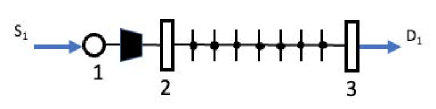
Figure 1: Single Discretized Pipe

IV Optimal Control Problem

The objective function for the optimal control problem (OCP) consists of the economic value generated by the pipeline operator through sales of energy and purchases of gas constituents, minus the operating cost of compressors. The objective function is of the form

$$\begin{split}R\!=\!\!\sum_{t\in T_{s}}\left(\sum_{i\in I}(\eta^{s}_{i}c_{H_{2},i}\!+\!(1-\eta^{s}_{i})c_{NG,i})q^{i,t}_{s}\!-\!\sum_{i\in W}C^{E}g_{i,t}^{E}\right)\!\!,\end{split}$$ (15a)

where $$c_{H_{2}} c_{NG} C^{E}$$ and denote supplier offer prices for H₂ and NG, and denotes the price that consumers bid for energy delivered through the mixed gas in $/MW. The operating cost for each compressor is determined using an adiabatic compression work expression [20], of form

$$W_{c}=\left(\frac{286.76\cdot\kappa_{ij}\cdot T}{G_{ij}{(\kappa_{ij}-1)}}\right)\left(\alpha_{ij}^{m}-1\right)\left|f^{c}_{ij}\right|.$$ (15b)

We approximate the terms in the left parentheses, comprised of physical parameters such as specific heat capacity ratio and specific gravity, as constants and denote the entire expression by $$K \zeta=0.07$$. The compressor cost is obtained by multiplying the total compressor work by a constant electricity price of $/kWh, resulting in

$$R_{c}=K\cdot\zeta\cdot\sum_{t_{n}}\sum_{ij\in C}f^{c,t}_{ij}\left(\sqrt{\alpha^{t}_{ij}}-1\right).$$ (15c)

The total objective function is a weighted sum of the economic cost and the operating cost with a weight $$\xi$$, of form

$$\min\enskip\mathbb{T^{\text{cost}}}=\xi R+(1-\xi)R_{c}.$$ (15d)

The scaling parameter can be used to prioritize on maximizing gas delivery or minimizing the operating cost. For $$\xi=0.5$$, the objective reduces to the sum of the two terms.

The complete optimization problem is formulated as:

$$\mathtt{OPT}~{}~{}\triangleq~{}~{} \min~{}~{}\mathbb{T^{\text{cost}}}~{}\text{in }\eqref{eq:total_objective},~{}\text{ -- subject to: }$$

equations (10) – (transport equations)

equations (12), (13) – (energy calculation)

equations (11) – (H₂ and NG nodal balance)

equations (14) – (network compatibility equations)

V Results

We solve the above problem for two examples that consist of a single pipe and an 8-node test network subject to variable boundary conditions and/or constraint bounds.

V-A Computational Implementation

Problem $\mathtt{OPT}$ is solved for both test cases using a NLP solver such as KNITRO [21] in the Julia based modeling language JuMP [22]. The problems are solved for a 24-hour time horizon with $T_{f}=24$ hours in a sequential manner. At first, the steady-state problem is solved by setting $\Delta T=T_{f}$ so that the time discretization is a single point. Thereafter, the steady-state solution is used as the initial guess for the full time discretization with $\Delta T=0.5\text{ or }1.0$ hours. Note that because the problem is non-convex, there are no guarantees of global optimality for the solution obtained by the NLP solver. Our model does ensure a feasible solution when a local optimum is attained, which is challenging for this problem.

V-B Single Pipe Case Study

Consider a single pipe of length $L=30$ km, diameter $D=0.9144$ m, and friction factor $\lambda=0.01$ connected with a compressor near the injection node (1) as shown in Fig. 1. We choose a discretization length of $\Delta L=10$ km to formulate the lumped element reduced model. The injection concentration $\eta^{s}$ is given as a time varying sinusoidal function

$$\eta^{s}=\eta^{s}_{0}+\delta\sin(2\pi\nu/T),$$ (16)

with $\eta^{s}_{0}=0.1$, $\delta=0.05$, and $\nu=2$. The function in equation (16) is shown as the node 1 concentration in Fig. 2(a). Pressure at the slack injection node 1 is fixed at $p^{s}=4.337$ MPa. The energy limit at the withdrawal node (3) is set at $g^{E,max}=8000$ MJ/s, and we bound the flow through the compressor at $f^{c}\leq 150$ kg/s. The pressure limits at the nodes are set at $p^{min}=3.0$ MPa and $p^{max}=6.0$ MPa.

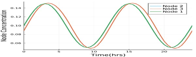
(a) Nodal concentration

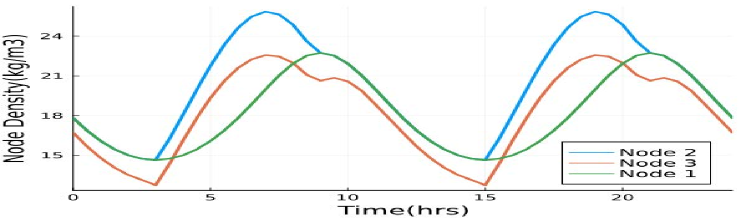
(b) Nodal density

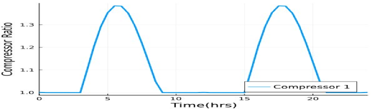
(c) Compressor Ratio

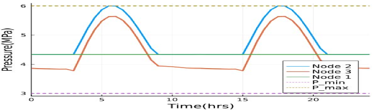
(d) Nodal Pressure

Figure 2: Optimal pressure, density, and concentration solutions for the single pipe case study.

The results from the optimization are plotted in Fig. 2 with profiles for nodal density, concentration, and pressure, and the boost ratio of the compressor. The nodal values are of interest, because these are observed by operators of the pipeline and by system users at custody transfer points. We first observe that the profiles are periodic with two cycles ($\nu=2.0$) in the 24 hour time period, and therefore discuss the trends in the first cycle ($T=0$ to $12$ hours) only. In Fig. 2(a), the H₂ concentrations at the three main nodes are plotted with time. The concentrations at node 1 (green) and 2 overlap because they are only connected by a compressor, whereas the concentration at the withdrawal node 3 (orange) is shifted to the right or lags behind because of the advective transport effect over the long pipe. The nodal density $\rho$ plotted in Fig. 2(b) is the sum of partial densities of H₂ and NG. The density at node 1 (green) follows a smooth sinusoid similar to the injection node concentration because the pressure at node 1 (slack) is fixed and the two quantities are related by equation (2f). Nodal density depends on both the concentration and pressure at the node, which we observe in Figures 2(a), 2(b), and 2(d) where there is a sharp increase in compressor pressure outlet (node 2) around $t=3.5$ hours, which increases until it reaches the upper bound $p=6.0$ MPa at $t=5.5$ hours and then begins to decrease. In contrast to that, the densities at compressor outlet and withdrawal node vary slowly, and reached their maxima at $t=7.5$ hours (see Fig. 2(b)). Observe also that the density at the withdrawal node (node 3) has a smaller local maximum near $t=9.5$ hours that results because the minimum in nodal concentration at the withdrawal node occurs at that time. The pressure drop across the pipe seen in Fig. 2(d) appears higher when the node concentrations are high, such as at $t=2.5$ hours or when injection and withdrawal flows are high, as at $t=10.5$ hours.

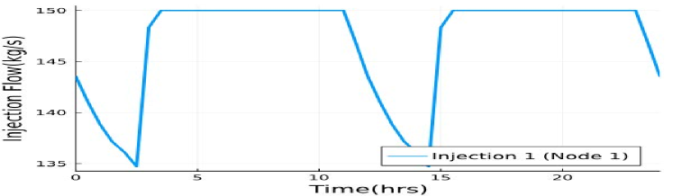
(a) Injection flow

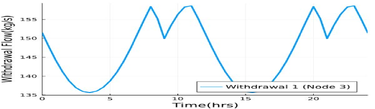
(b) Withdrawal flow

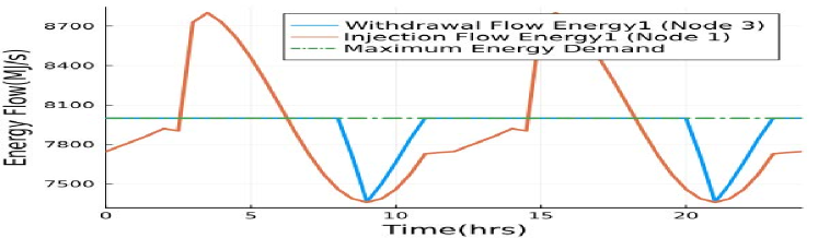
(c) Energy Flow

Figure 3: Optimal flow solutions for the single pipe case study.

Fig. 3 shows the variation in injection and withdrawal flow along with the energy delivered at the withdrawal node. Because the optimization solver seeks to maximize the energy delivered at the withdrawal node (see equation (15d)), the amount of energy delivered is equal to its upper bound limit at 8000 MJ/s, except for a short duration between $T=9.0$ to $10.5$ hours. This is because the H₂ injection concentration in Fig. 2(a) is so low that the energy content of the gas cannot meet the desired value of 8000 MJ/s without violating the compressor flow bound of 150 kg/s (see Fig. 3(c)). Notice that the injection flow and energy flow both increase sharply at around $T=2.5$ hours, but the energy injection begins to decrease subsequently because of the decrease in injection concentration. This is consistent with the pressure and node concentration profiles in Fig. 2(d) and Fig. 2(a), respectively. Similarly, the withdrawal flow in Fig. 3(b) is lower when nodal H₂ concentration is high and increases when the nodal concentrations begins to decrease at $T=3.5$ hours, until it is unable to match the maximum energy demand at $T=9.0$ hours, when it sharply decreases to minimize pressure drop, resulting in the compressor activity shown in Fig. 2(c). The withdrawal flow subsequently begins to slowly increase again to maximize the energy supply when the withdrawal node concentration begins increasing at $T=10.0$ hours. Another important observation is that the maximum energy demand at the withdrawal node is met more regularly than the amount of time the energy flowing into node 1 is above the desired delivery rate at node 3.

V-C 8-node Network Case Study

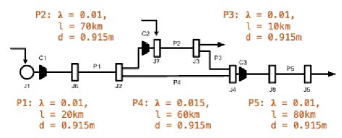
Figure 4: 8-node test pipeline network and parameters.

Next, we demonstrate our model using an 8-node gas network example that features a loop, as shown in Figure 4. The network has one slack node (J1), two injections (J1 and J7), and two withdrawals (J3 and J5) along with three compressors. The pressure and injection concentration at slack node J1 are fixed at $p=5.0$ MPa and $\eta^{s}=0.08$. Meanwhile, the injection concentration at node J7 is varied as a sinusoid of the form in equation (16), similar to the single-pipe case, with $\eta^{s}_{0}=0.05$, $\delta=0.01$, and $\nu=1$. We use a coarser time discretization of $\Delta T=1.0$ hour in this example, which results in 7536 variables and 7392 equality constraints. The compressor flow bounds are set at $f^{c,1}\leq 275$ kg/s, $f^{c,2}\leq 260$ kg/s and $f^{c,3}\leq 140$ kg/s. The pressure bounds and maximum energy demand are the same as in the single pipe example.

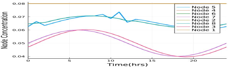
(a) Nodal concentration

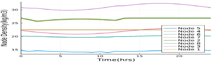
(b) Nodal density

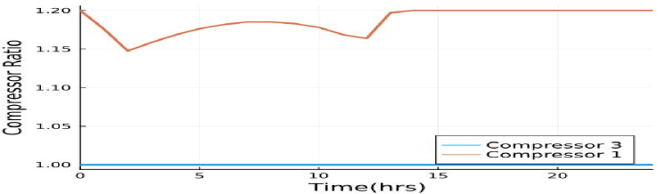
(c) Compressor Ratio

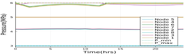
(d) Nodal Pressure

Figure 5: Optimal pressure, density, and concentration solutions for the 8-node test network.

The optimal solutions for the 8-node case study are shown in Fig. 5 and Fig. 6. Unlike for the single pipe case study, the profiles are less periodic and more non-uniform. A plausible explanation is that the nonlinearity of the nodal balance constraints in equations (11) and the presence of two sources with different H₂ injection concentrations cause complex interactions with delays. Nonetheless, we do observe that there is no gas flow through compressor C2 in the optimal solution, and that compressor C3 is inactive in the optimal solution because the pressure at the withdrawal node J5 is at its lower bound. We also observe that the binding constraint in the network which is always active is the upper bound on the compressor flow C3 ($f^{*c,3}=140$ kg/s). The pressure at J6 and J2 follow a similar trend where the compressor C1 is used to increase the pressure of injected gas from J1 (see Fig. 5(d) and Fig. 5(c)). The H₂ concentration at node J4 (cyan) is determined by the nodal mixing of gas with fixed concentration from node J2 (yellow) and gas with varying concentration from node J3 (pink) as seen in Fig. 5(a). In Fig. 6(b), the withdrawal flow at node J3 is sinusoidal, which balances the sinusoidal node concentration in Fig. 5(a) and results in constant withdrawal energy at 8000 MJ/s.

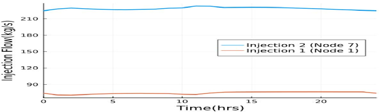
(a) Injection flow

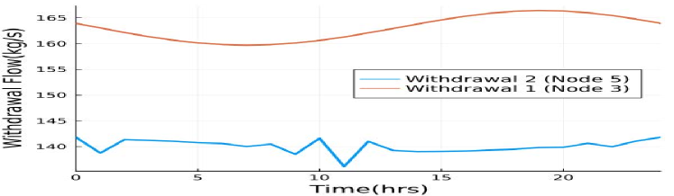
(b) Withdrawal flow

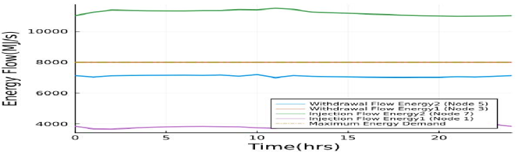
(c) Energy Flow

Figure 6: Optimal flow solutions for the 8-node test network.

VI Conclusion and Future Work

We formulate the challenging problem of model-predictive optimal control of hydrogen blending into natural gas pipeline networks subject to inequality constraints. Our numerical method employs a lumped parameter approximation to reduce the associated partial differential equations to a differential algebraic equation system that can be easily discretized and solved using nonlinear optimization solvers. We employ a circular time-discretization that is advantageous for time-periodic boundary conditions, parameters, and inequality constraint bound values. The key advance in this study is the optimization of time-varying withdrawals from the network, where the running objective function is formulated in terms of energy delivery to consumers and mass injection by suppliers of natural gas or hydrogen. This leads to a conceptually and computationally well-posed formulation, which enables numerical resolution of the complex behavior that arises from nonlinear interactions of inhomogeneous gas flows mixing throughout a pipeline network. Future studies will extend the setting to uncertain parameters and investigate economic questions by examining the dual solution.

References

- [1] Maciej Chaczykowski, Filip Sund, Paweł Zarodkiewicz, and Sigmund Mongstad Hope. Gas composition tracking in transient pipeline flow. J. Natural Gas Science & Engineering, 55:321–330, 2018.
- [2] Luke S. Baker, Saif R. Kazi, and Anatoly Zlotnik. Transitions from monotonicity to chaos in gas mixture dynamics in pipeline networks. PRX Energy, 2:033008, Aug 2023.
- [3] Firooz Tabkhi, Catherine Azzaro-Pantel, Luc Pibouleau, and Serge Domenech. A mathematical framework for modelling and evaluating natural gas pipeline networks under hydrogen injection. International journal of hydrogen energy, 33(21):6222–6231, 2008.
- [4] Mo Sodwatana, Saif R. Kazi, Kaarthik Sundar, and Anatoly Zlotnik. Optimization of hydrogen blending in natural gas networks for carbon emissions reduction. In 2023 American Control Conference (ACC), pages 1229–1236. IEEE, 2023.
- [5] Dries Haeseldonckx and William D’haeseleer. The use of the natural-gas pipeline infrastructure for hydrogen transport in a changing market structure. Internatl. J. Hydrogen Energy, 32(10-11):1381–1386, 2007.
- [6] Anatoly Zlotnik, Saif R. Kazi, Kaarthik Sundar, Vitaliy Gyrya, Luke Baker, Mo Sodwatana, and Yan Brodskyi. Effects of hydrogen blending on natural gas pipeline transients, capacity, and economics. In PSIG Annual Meeting, page 2312. PSIG, 2023.
- [7] Giulio Guandalini, Paolo Colbertaldo, and Stefano Campanari. Dynamic modeling of natural gas quality within transport pipelines in presence of hydrogen injections. Applied Energy, 185:1712–1723, 2017.
- [8] Kai Liu, Saif R. Kazi, Lorenz T. Biegler, et al. Dynamic optimization for gas blending in pipeline networks with gas interchangeability control. AIChE Journal, 66(5):e16908, 2020.
- [9] Marc W. Melaina, Olga Antonia, and Michael Penev. Blending hydrogen into natural gas pipeline networks: A review of key issues. NREL Tech. Rep., NREL/TP-5600-51995, 2013.
- [10] Bin Miao, Lorenzo Giordano, and Siew Hwa Chan. Long-distance renewable hydrogen transmission via cables and pipelines. International journal of hydrogen energy, 46(36):18699–18718, 2021.
- [11] Sebastian Schuster, Hans Josef Dohmen, and Dieter Brillert. Challenges of compressing hydrogen for pipeline transportation with centrifugal compressors. In Proceedings of Global Power and Propulsion Society, pages 2504–4400, 2020.
- [12] Zihang Zhang, Isam Saedi, Sleiman Mhanna, Kai Wu, and Pierluigi Mancarella. Modelling of gas network transient flows with multiple hydrogen injections and gas composition tracking. International Journal of Hydrogen Energy, 47(4):2220–2233, 2022.
- [13] Andrzej Witkowski, Andrzej Rusin, Mirosław Majkut, and Katarzyna Stolecka. Analysis of compression and transport of the methane/hydrogen mixture in existing natural gas pipelines. International Journal of Pressure Vessels and Piping, 166:24–34, 2018.
- [14] Henry H. Rachford and Richard G. Carter. Optimizing pipeline control in transient gas flow. In PSIG Annual Meeting, page 0004, 2000.
- [15] Sai Krishna Kanth Hari, Kaarthik Sundar, Shriram Srinivasan, Anatoly Zlotnik, and Russell Bent. Operation of natural gas pipeline networks with storage under transient flow conditions. IEEE Transactions on Control Systems Technology, 30(2):667–679, 2021.
- [16] Aleksandr Rudkevich, Anatoly Zlotnik, Xindi Li, Pablo Ruiz, et al. Evaluating benefits of rolling horizon model predictive control for intraday scheduling of a natural gas pipeline market. In 52nd Hawaii International Conference on System Sciences, pages 3627–3636, 2019.
- [17] Michael Herty, Jan Mohring, and Veronika Sachers. A new model for gas flow in pipe networks. Mathematical Methods in the Applied Sciences, 33(7):845–855, 2010.
- [18] Andrzej Osiadacz. Simulation of transient gas flows in networks. International J. Numerical Methods in Fluids, 4(1):13–24, 1984.
- [19] Sara Grundel, Lennart Jansen, Nils Hornung, et al. Model order reduction of differential algebraic equations arising from the simulation of gas transport networks. In Progress in Differential-Algebraic Equations: Deskriptor 2013, pages 183–205. Springer, 2014.
- [20] Kaarthik Sundar and Anatoly Zlotnik. State and parameter estimation for natural gas pipeline networks using transient state data. IEEE Transactions on Control Systems Technology, 27(5):2110–2124, 2018.
- [21] Richard H. Byrd, Jorge Nocedal, and Richard A. Waltz. Knitro: An Integrated Package for Nonlinear Optimization, pages 35–59. Springer US, Boston, MA, 2006.
- [22] Iain Dunning, Joey Huchette, and Miles Lubin. Jump: A modeling language for mathematical optimization. SIAM Review, 59(2):295–320, 2017.