A Certified Radius-Guided Attack Framework to Image Segmentation Models

Abstract

Image segmentation is an important problem in many safety-critical applications such as medical imaging and autonomous driving. Recent studies show that modern image segmentation models are vulnerable to adversarial perturbations, while existing attack methods mainly follow the idea of attacking image classification models. We argue that image segmentation and classification have inherent differences, and design an attack framework specially for image segmentation models. Our goal is to thoroughly explore the vulnerabilities of modern segmentation models, i.e., aiming to misclassify as many pixels as possible under a perturbation budget in both white-box and black-box settings.

Our attack framework is inspired by certified radius, which was originally used by defenders to defend against adversarial perturbations to classification models. We are the first, from the attacker perspective, to leverage the properties of certified radius and propose a certified radius guided attack framework against image segmentation models. Specifically, we first adapt randomized smoothing, the state-of-the-art certification method for classification models, to derive the pixel’s certified radius. A larger certified radius of a pixel means the pixel is theoretically more robust to adversarial perturbations. This observation inspires us to focus more on disrupting pixels with relatively smaller certified radii. Accordingly, we design a pixel-wise certified radius guided loss, when plugged into any existing white-box attack, yields our certified radius-guided white-box attack.

Next, we propose the first black-box attack to image segmentation models via bandit. A key challenge is no gradient information is available. To address it, we design a novel gradient estimator, based on bandit feedback, which is query-efficient and provably unbiased and stable. We use this gradient estimator to design a projected bandit gradient descent (PBGD) attack. We further use pixels’ certified radii and design a certified radius-guided PBGD (CR-PBGD) attack. We prove our PBGD and CR-PBGD attacks can achieve asymptotically optimal attack performance with an optimal rate. We evaluate our certified-radius guided white-box and black-box attacks on multiple modern image segmentation models and datasets. Our results validate the effectiveness of our certified radius-guided attack framework.

1 Introduction

Image segmentation (also called pixel-level classification) is the task of labeling pixels in an image such that pixels belonging to the same object are assigned a same label. Image segmentation is an important problem in many safety-critical applications such as medical imaging [1] (e.g., tumor detection), autonomous driving [2] (e.g., traffic sign detection). However, recent studies [3, 4, 5, 6, 7] showed that modern image segmentation models [8, 9, 10] are vulnerable to adversarial perturbations: A carefully designed imperceptible perturbation to a testing image can mislead an image segmentation model to misclassify a substantial number of pixels in this image. Such vulnerabilities would cause serious consequences in the safety-critical applications. For example, an attacker can attack a traffic sign prediction system such that a “STOP” sign image after segmentation will be misclassified as, e.g., “SPEED” or “LEFTTURN”—This causes safety issues. For another example, insurance companies often use their disease diagnosis systems to test medical images before reimbursing a medical claim. However, an attacker (e.g., an insider) can fool the disease diagnosis systems (e.g., no tumor diagnosed as tumor) by imperceptibly modifying the attacker’s medical images and sending fraud insurance claims—This causes insurance companies’ financial loss.

While these recent attack methods to image segmentation models have been proposed, they majorly follow the idea of attacking image classification models based on, e.g., the Fast Gradient Sign (FGSM) [11, 12] and Projected Gradient Descent (PGD) [13] attacks. However, we emphasize that image segmentation models and classification models have inherent differences: image classification models have a single prediction for an entire image, while image segmentation models have a prediction for each pixel. The per-pixel prediction can provide more information for an attacker to be exploited, e.g., an attacker can collectively leverage all pixels’ predictions to perform the attack. In this paper, we would like to design an optimized attack framework specially for image segmentation models by leveraging the pixels’ predictions. Specifically, given a target image segmentation model and a testing image, our goal is to generate an adversarial perturbation to this image under a perturbation budget, such that as many pixels as possible in the image are wrongly predicted by the target model.

To achieve the goal, our attack needs to first uncover the vulnerable pixels in the testing image, where a pixel is more vulnerable means it is easier to be misclassified when facing an adversarial perturbation, and then distributes the perturbation budget on more vulnerable pixels in order to misclassify more pixels. However, a key challenge is how can we inherently characterize the vulnerability of pixels. To address it, we are inspired by certified robustness/radius [14, 15, 16, 17, 18, 19, 20, 21, 22, 23, 24, 25, 26, 27, 28, 29, 30, 31, 32, 33, 34, 35, 36, 37, 38, 39, 40, 41, 42, 43, 44, 45]. Certified radius was originally used by defenders to guarantee the robustness of image classification models against adversarial perturbations. Given a classification model and a testing image, the certified radius of this image is the maximum (e.g., $l_{p}$) norm of a worst-case perturbation such that when the worst-case perturbation is added to the testing image, the perturbed image can be still accurately predicted by the classification model. In other words, a testing image with a larger/smaller certified radius indicates it is theoretically less/more vulnerable to adversarial perturbations. Though certified radius is derived mainly for doing the good, we realize that attackers, on the other hand, can also leverage it to do the bad in the context of image segmentation. Particularly, attackers can first attempt to obtain the certified radius of pixels, and use them to reversely reveal the inherently vulnerable pixels in the image. Then they can design better attacks using these vulnerable pixels.

Our work: We use the property of pixel’s certified radius and design the first certified radius-guided attack framework to image segmentation models. To thoroughly understand the vulnerabilities, we study both white-box and black-box attacks. However, there are several technical challenges: i) How can we obtain pixel-wise certified radius for modern image segmentation models? ii) How can we design an attack framework that is applicable in both white-box and black-box settings? iii) Furthermore, for the black-box attack, can we have guaranteed attack performance to make it more practical?

Obtaining pixel-wise certified radius via randomized smoothing: Directly calculating the pixel-wise certified radius for segmentation models is challenging. First, there exists no certification method for segmentation models; Second, though we may be able to adjust existing certification methods for image classification models to segmentation models (e.g., [14, 15, 16, 17, 18, 19, 20, 21, 22, 23, 24, 25, 26, 27, 28, 29, 30]), the computational overhead can be extremely high. Note that all the existing certification methods for base image classification models are not scalable to large models. To address the challenges, we propose to adopt randomized smoothing [33, 46], which is the state-of-the-art certification method for smoothed image classification models, and the only method that is scalable to large models. We generalize randomize smoothing to derive pixel-wise certified radius for image segmentation models (See Theorem 1).

Designing a certified radius-guided attack framework: A larger certified radius of a pixel indicates this pixel is theoretically more robust to adversarial perturbations. In other words, an attacker needs a larger perturbation to make the target image segmentation model misclassify this pixel. This observation motivates us to focus more on perturbing pixels with relatively smaller certified radii under a given perturbation budget. To achieve the goal, we design a certified radius-guide loss function, where we modify the conventional (pixel-wise) loss function in the target model by assigning each pixel a weight based on its certified radius. Specifically, a pixel with a large/smaller certified radius will be assigned a smaller/larger weight. By doing so, losses for pixels with smaller certified radii will be enlarged, and thus more pixels with be wrongly predicted with the given perturbation budget.

Certified radius-guided white-box attacks: In white-box attacks, an attacker has full knowledge of the target model, which makes gradient-based attacks possible. Our aim is then to increase our certified radius-guided loss and generate adversarial perturbations via a gradient-based white-box attack algorithm, e.g., the PGD attack [7, 13]. We emphasize that, as our pixel-wise certified radius is plugged into the loss function of the target model, any existing gradient-based white-box attack can be used as the base attack in our framework.

Certified radius-guided black-box attacks: In black-box attacks, an attacker cannot access the internal configurations of the target model. Hence, performing black-box attacks is much more challenging than white-box attacks, as no gradient information is available to determine the perturbation direction. Following the existing black-box attacks to image classification models [47, 48, 49], we assume the attacker knows pixels’ confidence scores by querying the target segmentation model. To design effective black-box attacks, one key step is to estimate the gradient of the attack loss with respect to the perturbation. Generally speaking, there are two types of approaches to estimate the gradients  [52]—deterministic methods and stochastic methods. The well-known deterministic method is the zeroth-order method (i.e., ZOO [53, 54]), and stochastic methods include natural evolutionary strategies (NES) [47], SimBA [55] and bandit [56, 57]. When performing real-world black-box attacks, query efficiency and gradient estimation accuracy are two critical factors an attacker should consider. However, ZOO is very query inefficient, while NES and SimBA are neither query efficient nor have accurate gradient estimation (More detailed analysis are in Section 4.3). Bandit methods, when appropriately designed, can achieve the best tradeoff. Moreover, as far as we know, bandit is the only framework, under which, we can derive theoretical bounds when the exact gradient is unknown. Based on these good properties, we thus use bandit as our black-box attack methodology.

Specifically, bandit is a family of optimization framework with partial information (also called bandit feedback) [58, 59, 60, 61, 62]. We notice that black-box attacks with only knowing pixels’ predictions naturally fit this framework. With it, we formulate the black-box attacks to image segmentation models as a bandit optimization problem. Our goal is to design a gradient estimator based on the model query and bandit feedback such that the regret (i.e., the difference between the expected observed loss through the queries and the optimal loss) is minimized. We first design a novel gradient estimator, which is query-efficient (2 queries per round) and accurate. Then, we design a projected bandit gradient descent (PBGD) attack algorithm based on our gradient estimator. As calculating pixels’ certified radii only needs to know pixels’ predictions, our derived pixel-wise certified radius can be seamlessly incorporated into the PBGD attack as well. With it, we further propose a certified radius-guided PBGD attack algorithm to enhance the black-box attack performance.

Theoretically guaranteed black-box attack performance: We prove that our novel gradient estimator is unbiased and stable. We further prove that our designed PBGD attack algorithm achieves a tight sublinear regret, which means the regret tends to be 0 with an optimal rate as the number of queries increases. Finally, our certified radius-guided PBGD attack also obtains a tight sublinear regret. Detailed theoretical results are seen in Section 4.4.

Evaluations: We evaluate our certified radius-guided white-box and black-box attacks on modern image segmentation models (i.e., PSPNet [8], PSANet [9], and HRNet [10]) and benchmark datasets (i.e., Pascal VOC [63], Cityscapes [64], and ADE20K [65]). In white-box attacks, we choose the state-of-the-art PGD [7, 13] attack as a base attack. The results show that our certified radius-guided PGD attack can substantially outperform the PGD attack. For instance, our attack can have a 50% relative gain over the PGD attack in reducing the pixel accuracy on testing images from the datasets. In black-box attacks, we show that our gradient estimator achieves the best trade-off among query-efficiency, accuracy, and stability, compared with the existing ones. The results also demonstrate the effectiveness of our PBGD attack and that incorporating pixel-wise certified radius can further enhance the attack performance.

We also evaluate the state-of-the-art empirical defense FastADT [66] and provable defense SEGCERTIFY [67] against our attacks. To avoid the sense of false security [68], we mainly defend against our white-box CR-PGD attack. Our finding is these defenses can mitigate our attack to some extent, but are still not effective enough. For example, with an $l_{2}$ perturbation as 10 on Pascal VOC, the pixel accuracy with SEGCERTIFY and FastADT are 22% and 41%, respectively, while the clean pixel accuracy is 95%. Our defense results thus show the necessity of designing stronger defenses in the future.

Our key contributions are summarized as follows:

• We propose a certified radius-guide attack framework to study both white-box and black-box attacks to image segmentation models. This is the first work to use certified radius for an attack purpose. Our framework can be seamlessly incorporated into any existing and future loss-based attacks.

• We are the first to study black-box attacks to image segmentation models based on bandits. We design a novel gradient estimator for black-box attacks that is query-efficient, and provably unbiased and stable. Our black-box attacks also achieve a tight sublinear regret.

• Evaluations on modern image segmentation models and datasets validate the effectiveness of our certified radius-guided attacks and their advantages over the compared ones mainly for image classification methods.

2 Background and Problem Setup

2.1 Image Segmentation

Image segmentation is the task of labeling pixels of an image, where pixels belonging to the same object (e.g., human, tree, car) aim to be classified as the same label. Formally, given an input image $\bm{x}=\{x_{n}\}_{n=1}^{N}\subset\mathcal{X}$ with $N$ pixels and groundtruth pixel labels $y=\{y_{n}\}_{n=1}^{N}$, where each pixel $x_{n}$ has a label $y_{n}$ from a label set $\mathcal{Y}$, an image segmentation model learns a mapping $F_{\theta}:\mathcal{X}\rightarrow\mathbb{P}^{N\times|\mathcal{Y}|}$, parameterized by $\theta$, where each row in $\mathbb{P}$ is the set of probability distributions over $\mathcal{Y}$, i.e., the sum of each row in $\mathbb{P}$ equals to 1. Different image segmentation methods design different loss functions to learn $F_{\theta}$. Suppose we have a set of training images $\mathbb{D}_{tr}=\{(x,y)\}$, a common way to learn $F_{\theta}$ is by minimizing a pixel-wise loss function $L$ defined on the training set as follows:

$$\small{\min_{\theta}}\sum_{\small(x,y)\in\mathbb{D}_{tr}}L(F_{\theta}(x),y)=-\sum_{(x,y)\in\mathbb{D}_{tr}}\sum_{n=1}^{N}1_{y_{n}}\odot\log F_{\theta}(x)_{n},$$ (1)

where we use the cross entropy as the loss function. $1_{y_{n}}$ is an $|\mathcal{Y}|$-dimensional indicator vector whose $y_{n}$-th entry is 1, and 0 otherwise. $\odot$ is the element-wise product. After learning $F_{\theta}$, giving a testing image $\underline{x}$, each pixel $\underline{x}_{n}$ is predicted a label $\hat{y}_{n}=\arg\max_{j}F_{\theta}(\underline{x})_{n,j}$.

2.2 Certified Radius

We introduce the certified radius achieved via state-of-the-art randomized smoothing methods [33, 46]. Certified radius was originally derived to measure the certified robustness of an image classifier against adversarial perturbations. Generally speaking, for a testing image, if it has a larger certified radius under the classifier, then it is provably more robust to adversarial perturbations.

Suppose we are given a testing image $x$ with a label $y$, and a (base) soft classifier $f$, which maps ${x}$ to confidence scores. Randomized smoothing first builds a smoothed soft classifier $g$ from the base $f$ and then calculates the certified radius for $x$ on the smoothed soft classifier $g$. Specifically, given a noise distribution $\mathcal{D}$, $g$ is defined as:

$$g(x)=\mathbb{E}_{\beta\sim\mathcal{D}}[f(x+\beta)],$$ (2)

where $g(x)_{c}$ is the probability of the noisy $x+\beta$ predicts to be the label $c$, with the noise $\beta$ sampled from $\mathcal{D}$.

Assuming that $g(x)$ assigns to $x$ the true label $y$ with probability $p_{A}=g(x)_{y}$, and assigns to $x$ the “runner-up” label $y^{\prime}$ with probability $p_{B}=\max_{y^{\prime}\neq y}g(x)_{y^{\prime}}$. Suppose $\mathcal{D}$ is a Gaussian distribution with mean 0 and variance $\sigma^{2}$. Then, authors in [33, 46] derive the following tight certified radius of the smoothed soft classifier $g$ for the testing image $x$ against an $l_{2}$ perturbation:

$$cr(x)=\frac{\sigma}{2}[\Phi^{-1}(p_{A})-\Phi^{-1}(p_{B})],$$ (3)

where $\Phi^{-1}$ is the inverse of the standard Gaussian cumulative distribution function (CDF). That is, $g$ provably has the correct prediction $y$ for $x$ over all adversarial perturbations $\delta$, i.e., $\arg\max_{c}g(x+\delta)_{c}=y$, when $||\delta||_{2}\leq cr(x)$. Note that calculating the exact probabilities $p_{A}$ and $p_{B}$ is challenging. Authors in [33, 46] use the Monte Carlo sampling algorithm to estimate a lower bound $\underline{p_{A}}$ of $p_{A}$ and an upper bound $\overline{p_{B}}$ of $p_{B}$ with arbitrarily high probability over the samples. They further set $\overline{p_{B}}=1-\underline{p_{A}}$ for simplicity. Then, $cr(x)=\sigma\Phi^{-1}(\underline{p_{A}})$.

2.3 Bandit

In the continuous optimization setting, the bandit method optimizes a black-box function over an infinite domain with feedback. The black-box function means the specific form of the function is not revealed but its function value can be observed. Due to this property, bandit can be a natural tool to design black-box algorithms. Next, we describe the three components: action, (bandit) feedback, and goal, in a bandit optimization problem.

• Action: A learner plans to maximize a time-varying reward function $r_{t}(\cdot)$ with $T$ rounds’ evaluations. In each round $t$, the learner selects an action $x_{t}$ from a action space, $\mathcal{S}$, which is often defined as a convex set.

• Feedback: When the learner performs an action $x_{t}$ and submits the decision to the environment in round $t$, he will observe a reward $r_{t}(x_{t})$ at $x_{t}$. As the observed information about the reward function $r_{t}$ is partial (i.e., only the function value instead of the function itself) and incomplete (the function value may be noisy), the observed information is often called bandit feedback.

• Goal: As no full information in advance, the learner uses regret to measure the performance of his policy $\mathcal{P}$. The goal of the learner is to design a policy $\mathcal{P}$ to minimize the regret, which is defined as the gap between the expected cumulative rewards achieved by the selected actions and the maximum cumulative rewards achieved by the optimal action in hindsight, i.e.,

  $$R_{\mathcal{P}}(T)=\mathbb{E}[\sum_{t=1}^{T}r_{t}(x_{t})-\max_{x\in\mathcal{S}}r_{t}(x)],$$ (4)

  where the expectation is taken over the randomness in the policy $\mathcal{P}$. When the policy $\mathcal{P}$ achieves a sublinear regret (i.e., $R_{\mathcal{P}}(T)=o(T)$), we say it is asymptotically optimal as the incurred regret disappears when $T$ is large enough, i.e., $\lim_{T\to\infty}R_{\mathcal{P}}(T)/T=0$.

2.4 Problem Setup

Suppose we have a target image segmentation model $F_{\theta}$, a testing image $x=\{x_{n}\}_{n=1}^{N}$ with true pixel labels $y=\{y_{n}\}_{n=1}^{N}$. We consider that an attacker can add an adversarial perturbation $\delta=\{\delta_{n}\}_{n=1}^{N}$ with a bounded $l_{p}$-norm $\epsilon$ to $x$, i.e., $\delta\in\Delta=\{\delta:||\delta||_{p}\leq\epsilon\}$. The attacker’s goal is to maximally mislead $F_{\theta}$ on the perturbed testing image $x+\delta$, i.e., making as many pixels as possible wrongly predicted by $F_{\theta}$. Formally,

$$\max_{\delta}\sum_{n=1}^{N}1[\arg\max_{c\in\mathcal{Y}}F_{\theta}(x+\delta)_{n,c}\neq y_{n}],\,\textrm{s.t., }\delta\in\Delta.$$ (5)

The above problem is challenging to solve in that the indicator function $1[\cdot]$ is hard to optimize. In practice, the attacker will solve an alternative optimization problem that maximizes an attack loss to find the perturbation $\delta$. S/He can use any attack loss in the existing works [3, 4, 5, 6, 7]. For instance, s/he can simply maximize the loss function $L$:

$$\max_{\delta}L(F_{\theta}(x+\delta),y)=\sum_{n=1}^{N}L(F_{\theta}(x+\delta)_{n},y_{n}),\textrm{s.t., }\delta\in\Delta.$$ (6)

In this paper, we consider both white-box attacks and black-box attacks to image segmentation models.

• White-box attacks: An attacker knows the full knowledge about $F_{\theta}$, e.g., model parameters $\theta$, architecture.

• Black-box attacks: An attacker has no knowledge about the internal configurations of $F_{\theta}$, and s/he only knows the confidence scores $F_{\theta}(x_{q})$ via querying $F_{\theta}$ with an input $x_{q}$, following the existing black-box attacks to image classification models [47, 48, 49].

3 Certified Radius Guided White-Box Attacks to Image Segmentation

3.1 Overview

Existing white-box attacks to image segmentation models majorly follow the idea of attacking image classification models [12, 13]. However, these attack methods are suboptimal. This is because the per-pixel prediction in segmentation models can provide much richer information for an attacker to be exploited, while classification models only have a single prediction for an entire image. We propose to exploit the unique pixel-wise certified radius information from pixels’ predictions. We first observe an inverse relationship between a pixel’s certified radius and the assigned perturbation to this pixel (See Figure 1) and derive pixel-wise certified radius via randomized smoothing [33, 46]. Then, we assign each pixel a weight based on its certified radius, and design a novel certified radius-guided attack loss, where we incorporate the pixel weights into the conventional attack loss. Finally, we design our certified radius-guided white-box attack framework to image segmentation models based on our new attack loss.

3.2 Attack Design

Our attack is inspired by certified radius. We first define our pixel-wise certified radius that is customized to image segmentation models.

Definition 1 (Pixel-wise certified radius).

Given a base (or smoothed) image segmentation model $F_{\theta}$ (or $G_{\theta}$) and a testing image $x$ with pixel labels ${y}$. We define certified radius of a pixel $x_{n}$, i.e., $cr(x_{n})$, as the maximal value, such that $F_{\theta}$ (or $G_{\theta}$) correctly predicts the pixel $x_{n}$ against any adversarial perturbation $\delta$ when its (e.g., $l_{p}$) norm is not larger than this value. Formally,

$$cr(x_{n})=\max r,$$

$$\textrm{s.t. }\arg\max_{c\in\mathcal{Y}}G_{\theta}(x+\delta)_{n,c}=y_{n},\forall||\delta||_{p}\leq r.$$ (7)

From Definition 1, the certified radius of a pixel describes the extent to which the image segmentation model can provably has the correct prediction for this pixel against the worst-case adversarial perturbation. Based on this, we have the following observation that reveals the inverse relationship between the pixel-wise certified radius and the perturbation when designing an effective attack.

Observation 1: A pixel with a larger (smaller) certified radius should be disrupted with a smaller (larger) perturbation on the entire image. If a pixel has a larger certified radius, it means this pixel is more robust to adversarial perturbations. To wrongly predict this pixel, an attacker should allocate a larger perturbation. In contrast, if a pixel has a smaller certified radius, this pixel is more vulnerable to adversarial perturbations. To wrongly predict this pixel, an attacker just needs to allocate a smaller perturbation. Thus, to design more effective attacks with limited perturbation budget, an attack should avoid disrupting pixels with relatively larger certified radii, but focus on pixels with relatively smaller certified radii.

With the above observation, our attack needs to solve three closely related problems: i) How to obtain the pixel-wise certified radius? ii) How to allocate the perturbation budget in order to perturb the pixels with smaller certified radii? and iii) How to generate adversarial perturbations to better attack image segmentation models? To address i), we adopt the efficient randomized smoothing method [33, 46]. To address ii), we design a certified-radius guided attack loss, by maximizing which an attacker will put more effort on perturbing pixels with smaller certified radii. To address iii), we design a certified radius-guide attack framework, where any existing loss-based attack method can be adopted as the base attack.

((a)) Raw image

((b)) True seg. labels

((c)) PGD pert. image

((d)) PGD perturbation

((e)) CR-PGD pert. img.

((f)) CR-PGD perturba.

((g)) PGD predictions

((h)) CR-PGD preds.

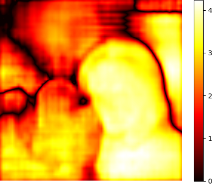
((i)) Pixel-wise CR

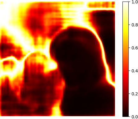
((j)) Pixel weights

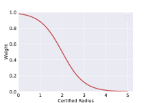
((k)) Certified radius vs. weight

Figure 1: (a)-(j) Illustration of our certified radius guided $l_{2}$ PGD attack on a random image in Pascal VOC. We observe that using pixels’ certified radii, our CR-PGD attack focuses more on perturbing pixels with relatively smaller certified radii, while PGD does not. Thus, our CR-PGD can misclassify more pixels than PGD. Regarding the inverse relationship in our observations: In (i), the left-bottom pixels have relatively larger certified radii, while the top-left/middle pixels have relatively smaller certified radii. Then, CR-PGD in (f) assigns less perturbations on the left-bottom region, but more perturbations on the top-left/middle region of the image. In contrast, PGD in (d) assigns more perturbations on the left-bottom region, but less on the top-lef/middle region. As a result, CR-PGD in (h) causes most pixels at the top-lef/middle to be misclassified, but PGD in (g) does not. (k) Relationship between pixel-wise certified radius and pixel weight in Equation 10, where $a=2$ and $b=-4$.

3.2.1 Deriving the pixel-wise certified radius via randomized smoothing

Directly calculating the pixel-wise certified radius for segmentation models faces two challenges: no certification method exists; and adjusting existing certification methods for (base) image classification models to segmentation models has extremely high computational overheads. For instance, one can use the approximate local Lipschitz proposed in [69]. However, as our results shown in Section 6, it is infeasible to apply [69] to calculate certified radius for segmentation models.

To address these challenges, we adapt the state-of-the-art randomized smoothing-based efficient certification method [33, 46] for smoothed image classification models. Specifically, we first build a smoothed image segmentation model for the target segmentation model and then derive the pixel-wise certified radius on the smoothed model via randomized smoothing as below:

Theorem 1.

Given an image segmentation model $F_{\theta}$ and a testing image $x$, we build a smoothed segmentation model as $G_{\theta}(x)={\mathbb{E}_{\beta\sim\mathcal{N}(0,{\sigma^{2}}I)}}F_{\theta}(x+\beta)$. Then for each pixel $x_{n}$, its certified radius for $l_{2}$ perturbation is:

$$cr(x_{n})=\sigma\Phi^{-1}(\max_{c}G_{\theta}(x)_{n,c}).$$ (8)

Proof.

See Appendix A.4. ∎

Remark 1: Theorem 1 generalizes randomized smoothing to segmentation models. In practice, however, obtaining the exact value of $\max_{c}G_{\theta}(x)_{n,c}$ is computationally challenging due to the random noise $\beta$. Here, we use the Monte Carlo sampling algorithm as  [33, 46] to estimate its lower bound. Specifically, we first sample a set of, say $M$, noises $\{\beta_{1},\beta_{2},\cdots,\beta_{M}\}$ from the Gaussian distribution $\mathcal{N}(0,\sigma^{2}I)$ and then use the empirical mean $\hat{G}_{\theta}(x)=\frac{1}{M}\sum_{i=1}^{M}F_{\theta}(x+\beta_{j})$ to estimate the lower bound as $\max_{c}\hat{G}_{\theta}(x)_{n,c}$. In contrast to the tight certified radius obtained in Equation 3 for image classification models, the pixel-wise certified radius in Equation 8 cannot guarantee to be tight for image segmentation models. Note that our goal is not to design a better defense that requires larger certified radii. Instead, we leverage the order of pixels’ certified radii to identify pixels’ relative robustness/vulnerability against adversarial perturbations, whose information is used to design more effective attacks.

Remark 2: The pixel-wise certified radius derived for $l_{2}$ perturbations in Equation 8 suffices to be used for other common norm-based, e.g., $l_{1}$ and $l_{\infty}$, perturbations. This is because a pixel with a larger $l_{2}$ certified radius also has a larger $l_{1}$ and $l_{\infty}$ certified radius, thus more robust against $l_{1}$ and $1_{\infty}$ perturbations.

Remark 3: The rationale of using randomized smoothing for certification is that, when an image A is intrinsically more robust than an image B on the base model against adversarial perturbation, then adding a small noise to these two images, the noisy A is still more robust than the noisy B on the smoothed model against adversarial perturbation. Moreover, the smoothed model has close certified radius under a small noise (i.e., a small $\sigma$) as the base model (on which certified radius is challenging to compute). Hence, a pixel’s certified radius on the smoothed model indicates its robustness on the base model as well.

3.2.2 Designing a certified radius-guided attack loss

After obtaining the certified radii of all pixels, a naive solution is that the attacker sorts pixels’ certified radii in an ascending order, and then perturbs the pixels one-by-one from the beginning until reaching the perturbation budget. However, this solution is both computationally intensive—as it needs to solve an optimization problem for each pixel; and suboptimal—as all pixels collectively make predictions for each pixel and perturbing a single pixel could affect the predictions of all the other pixels.

Here, we design a certified radius-guided attack loss that assists to automatically find the “ideal” pixels to be perturbed. We observe that the attack loss in Equation 6 is defined per pixel. Then, we propose to modify the attack loss in Equation 6 by associating each pixel with a weight and multiplying the weight with the corresponding pixel loss, where the pixel weight is correlated with the pixel’s certified radius. Formally, our certified radius-guided attack loss is defined as follows:

$$\small L_{cr}(F_{\theta}(x),y)=\frac{1}{N}\sum_{{n}=1}^{N}w(x_{n})\cdot L(F_{\theta}(x)_{n},y_{n}),$$ (9)

where $w(x_{n})$ is the weight of the pixel $x_{n}$. Note that when setting all pixels with a same weight, our certified radius-guided loss reduces to the conventional loss.

Next, we show the inverse relationship between the pixel-wise certified radius and pixel weight; and define an example form of the pixel weight used in our paper.

Observation 2: A pixel with a larger (smaller) certified radius should be assigned a smaller (larger) weight in the certified radius-guided loss. As shown in Observation 1, we should perturb more pixels with smaller certified radii, as they are more vulnerable. That is, we should put more weights on pixels with smaller certified radii to enlarge these pixels’ losses—making these pixels easier to be misclassified with perturbations. By doing so, the image segmentation model will wrongly predict more pixels with a given perturbation budget. In contrast, we should put smaller weights on pixels with larger certified radii, in order to save the usage of the budget.

There are many different ways to assign the pixel weight such that $w(x_{n})\sim\frac{1}{cr(w_{n})}$ based on Observation 2. In this paper, we propose to use the following form:

$$w(x_{n})=\frac{1}{1+\exp(a\cdot cr(x_{n})+b)},$$ (10)

where $a$ and $b$ are two scalar hyperparameters. Figure 1(k) illustrates the relationship between the pixel-wise certified radius and pixel weight defined in Equation 10, where $a=2$ and $b=-4$. We can observe that the pixel weight is exponentially decreased as the certified radius increases. Such a property can ensure that most of the pixels with smaller radii will be perturbed (See Figure 5) when performing the attack.

We emphasize that our weight design in Equation 10 is not optimal; actually due to the non-linearity of neural network models, it is challenging to derive optimal weights. Moreover, as pointed out [13], introducing randomness can make the attack more effective. Our smoothed segmentation model based weight design introduces randomness into our attack loss, which makes our attack harder to defend against, as shown in our results in Section 5.4.

3.2.3 Certified radius-guided white-box attacks to generate adversarial perturbations

We use our designed certified radius-guided attack loss to generate adversarial perturbations to image segmentation models. Note that we can choose any existing white-box attack as the base attack. In particular, given the attack loss from any existing white-box attack, we only need to modify our attack loss by multiplying the pixel weights with the corresponding attack loss. For instance, when we use the PGD attack [13] as the base attack method, we have our certified radius-guided PGD (CR-PGD) attack that iteratively generates adversarial perturbations as follows:

$$\delta=\textrm{Proj}_{\Delta}(\delta+\alpha\cdot\nabla_{\delta}L_{cr}(F_{\theta}(x+\delta),y)),$$ (11)

where $\alpha$ is the learning rate in PGD, $\Delta=\{\delta:||\delta||_{p}\leq\epsilon\}$ is the allowable perturbation set, and $\textrm{Proj}_{\Delta}$ projects the adversarial perturbation to the allowable set $\Delta$. The final adversarial perturbation is used to perform the attack.

Figure 1 illustrates our certified radius-guided attack framework to image segmentation models, where we use the $l_{2}$ PGD attack as the base attack method. Algorithm 1 in Appendix details our CR-PGD attack. Comparing with PGD, the computational overhead of our CR-PGD is calculating the pixel-wise certified radius with a small set of $M$ sampled noises (every INT iterations and INT is a predefined parameter in Algorithm 1 in Appendix), which only involves making predictions on $M$ noisy samples and is very efficient. Note that the predictions are independent and can be also parallelized. Thus, PGD and CR-PGD have the comparable computational complexity. We also show the detailed time comparison results in Section 5.2.

4 Certified Radius Guided Black-Box Attacks to Image Segmentation via Bandit

4.1 Motivation of Using Bandit

In black-box attacks, an attacker can only query the target image segmentation model to obtain pixels’ confidence scores. A key challenge in this setting is that no gradient information is available, and thus an attacker cannot conduct the (projected) gradient descent like white-box attacks [11, 13, 70] to determine the perturbation directions. A common way to address this is converting black-box attacks with partial feedback (i.e., confidence scores) to be the gradient estimation problem, solving which the standard (projected) gradient descent based attack can then be applied. Existing gradient estimate methods [52] can be classified as deterministic methods (e.g., zero-order optimization, ZOO [53, 54]) and stochastic methods (e.g., NES [47], SimBA [55], and bandit [56, 57]). To perform real-world black-box attacks, query efficiency and gradient estimation accuracy (in terms of unbiasedness and stability) are two critical factors. ZOO (See Equation 13) is accurate but query inefficient, while NES and SimBA are neither accurate nor query efficient. In contrast, bandit can achieve the best tradeoff  [58, 73] when the gradient estimator is appropriately designed.

4.2 Overview

Inspired by the good properties of bandits, we formulate the black-box attacks to image segmentation models as a bandit optimization problem. However, designing an effective bandit algorithm for solving practicable black-box attacks faces several technical challenges: 1) It should be query efficient; 2) it should estimate the gradient accurately; and 3) the most challenging, it should guarantee the attack performance to approach the optimal as the query number increases. We aim to address all these challenges. Specifically, we first design a novel gradient estimator with bandit feedback and show it only needs 2 queries per round. We also prove it is unbiased and stable. Based on our estimator, we then propose projected bandit gradient descent (PBGD) to construct the perturbation. We observe that the pixel-wise certified radius can be also derived in the considered black-box setting and be seamlessly incorporated into our PBGD based attack algorithm. Based on this observation, we further design a certified radius-guided PBGD (CR-PBGD) attack to enhance the black-box attack performance. Finally, we prove that our bandit-based attack algorithm achieves a tight sublinear regret, meaning our attack is asymptotically optimal with an optimal rate. The theoretical contributions of our regret bound can be also seen in Appendix A.7.

4.3 Attack Design

4.3.1 Formulating black-box attacks to image segmentation models as a bandit optimization problem

In the context of leveraging bandits to design our black-box attack, we need to define the attacker’s action, (bandit) feeback, and goal. Suppose there are $T$ rounds, which means an attacker will attack the target image segmentation model up to $T$ rounds. In each round $t\in\{1,2,\cdots,T\}$:

• Action: The attacker determines a perturbation $\delta^{(t)}\in\Delta$ via a designed attack algorithm $\mathcal{A}$.

• Feedback: By querying the target model with the perturbed image $x+\delta^{(t)}$, attacker observes the corresponding attack loss $L(\delta^{(t)})$ at the selected perturbation $\delta^{(t)}$.

• Goal: As the attacker only has the bandit feedback $L(\delta^{(t)})$ at the selected perturbation $\delta^{(t)}$, the attack algorithm $\mathcal{A}$ will incur a regret, which is defined as the expected difference between the attack loss at $\delta^{(t)}$ brought by $\mathcal{A}$ and the maximum attack loss in hindsight. Let $R_{\mathcal{A}}(T)$ be the cumulative regret after $T$ rounds, then the regret is calculated as

  $$\small R_{\mathcal{A}}(T)=\sum_{t=1}^{T}\mathbb{E}[L(\delta^{(t)})]-\max_{\delta\in\Delta}\sum_{t=1}^{T}L(\delta),$$ (12)

  where the expectation is taken over the randomness from $\mathcal{A}$. The attacker’s goal to minimize the regret.

Now our problem becomes: how does an attacker design an attack algorithm that utilizes the bandit feedback via querying the target model, and determine the adversarial perturbation to achieve a sublinear regret? There are several problems to be solved: (i) How to accurately estimate the gradient (i.e., unbiased and stable) in order to determine the perturbation? (ii) How to make black-box attacks query-efficient? (iii) How can we achieve a sublinear regret bound? We propose novel gradient estimation methods to solve them.

4.3.2 Two-point gradient estimation with bandit feedback

We first introduce two existing gradient estimators, i.e., the deterministic method-based ZOO [53, 54] and stochastic bandit-based one-point gradient estimator (OPGE) [74, 75, 73], and show their limitations. We do not show the details of NES [47] and SimBA [55] because they are neither accurate nor query efficient. Then, we propose our two-point gradient estimator.

ZOO. It uses the finite difference method [76] and determinately estimates the gradient vector element-by-element. Specifically, given a perturbation $\delta$, ZOO estimates the gradient of the $i$-th element, i.e., $\nabla L(\delta)_{i}$, as

$$\hat{g}^{ZOO}_{i}=\nabla L(\delta)_{i}\approx\frac{L(\delta+\gamma e_{i})-L(\delta-\gamma e_{i})}{2\gamma},$$ (13)

where $\gamma$ is a small positive number and $e_{i}$ is a standard basis vector with the $i$-th element be 1 and 0 otherwise.

ZOO is an unbiased gradient estimator. However, it faces two challenges: (i) It requires a sufficiently large number of queries to perform the gradient estimation, which is often impracticable due to a limited query budget. Specifically, ZOO depends on two losses $L(\delta+\gamma e_{i})$ and $L(\delta-\gamma e_{i})$, which is realized by querying the target model twice using the two points $\delta+\gamma e_{i}$ and $\delta-\gamma e_{i}$, and estimates the gradient of a single element $i$ per round. To estimate the gradient vector of $N$ elements, ZOO needs $2N$ queries per round. As the number of pixels $N$ in an image is often large, the total number of queries often exceeds the attacker’s query budget. (ii) It requires the loss function $L$ to be differentiable everywhere, while some loss functions, e.g., hinge loss, is nondifferentiable.

One-point gradient estimator (OPGE). It estimates the whole gradient in a random fashion. It first defines a smoothed loss $\hat{L}(\delta)$ of the loss $L(\delta)$ at a given perturbation $\delta$ as follows:

$$\hat{L}(\delta)=\mathbb{E}_{\bm{v}\in\mathcal{B}_{p}}[L(\delta+\gamma\bm{v})],$$ (14)

where $\mathcal{B}_{p}$ is a unit $l_{p}$-ball, i.e., $\mathcal{B}_{p}=\{u:||u||_{p}\leq 1\}$, and $v$ is a random vector sampling from $\mathcal{B}_{p}$. Then, by observing that $\hat{L}(\delta)\approx L(\delta)$ when $\gamma$ is sufficiently small, OPGE uses the gradient of $\hat{L}(\delta)$ to approximate $L(\delta)$. Specifically, the estimated gradient $\hat{L}(\delta)$ has the following form [74, 75, 73]:

$$\small\hat{g}^{OPGE}=\nabla\hat{L}(\delta)=\mathbb{E}_{\bm{u}\in\mathcal{S}_{p}}[\frac{N}{\gamma}L(\delta+\gamma\bm{u})\bm{u}],$$ (15)

where $\mathcal{S}_{p}$ is a unit $l_{p}$-sphere, i.e., $\mathcal{S}_{p}=\{u:||u||_{p}=1\}$. To calculate the expectation in Equation 15, OPGE simply samples a single $\hat{u}$ from $\mathcal{S}_{p}$ and estimates the expectation as $\frac{N}{\gamma}L(\delta+\gamma\hat{u})\hat{u}$. As OPGE only uses a point $\delta+\gamma\hat{u}$ to obtain the feedback $L(\delta+\gamma\hat{u})$, it is called one-point gradient estimator.

OPGE is extremely query-efficient as the whole gradient is estimated with only one query (based on one point $\delta+\gamma\hat{u}$). The gradient estimator $\hat{g}^{OPGE}$ is differentiable everywhere even when the loss function $L$ is non-differentiable. It is also an unbiased gradient estimation method, same as ZOO. However, OPGE has two key disadvantages: (i) Only when $\gamma$ is extremely small can $\hat{L}(\delta)$ be close to $L(\delta)$. In this case, the coefficient $N/\gamma$ would be very large. Such a phenomenon will easily cause the updated gradient out of the feasible image space $[0,1]^{N}$. (ii) The estimated gradient norm is unbounded as it depends on $\gamma$, which will make the estimated gradient rather unstable when only a single $\hat{u}$ is sampled and used.

The proposed two-point gradient estimator (TPGE). To address the challenges in OPGE, we propose a two-point gradient estimator (TPGD). TPGD combines the idea of ZOO and OPGE: On one hand, similar to OPGE, we build a smoothed loss function to make the gradient estimator differentiable everywhere and estimate the whole gradient at a time; On the other hand, similar to ZOO, we use two points to estimate the gradient, in order to eliminate the dependency caused by $\gamma$, thus making the estimator stable and correct. Specifically, based on Equation 15, we first set $u$ as its negative form $-u$, which also belongs to $\mathcal{S}_{p}$, and have $\nabla\hat{L}(\delta)=\mathbb{E}_{\bm{u}\in\mathcal{S}_{p}}[\frac{N}{\gamma}L(\delta-\gamma\bm{u})(-\bm{u})]$. Combining it with Equation 15, we have the estimated gradient as:

$$\small\hat{g}^{TPGE}=\nabla\hat{L}(\delta)=\underset{\bm{u}\in\mathcal{S}_{p}}{\mathbb{E}}[\frac{N}{2\gamma}\big{(}L(\delta+\gamma\bm{u})-L(\delta-\gamma\bm{u})\big{)}\bm{u}].$$ (16)

The properties of $\hat{g}^{TPGE}$ are shown in Theorem 2 (See Section 4.4). In summary, $\hat{g}^{TPGE}$ is an unbiased gradient estimator and has a bounded gradient norm independent of $\gamma$. An unbiased gradient estimator is a necessary condition for the estimated gradient to be close to the true gradient; and a bounded gradient norm can make the gradient estimator stable.

TABLE I: Comparing ZOO, NES, OPGE, and TPGE.

Method	ZOO	NES	SimBA	OPGE	TPGE
Type	Deter.	Stoc.	Stoc.	Stoc.	Stoc.
#Queries per round	2#pixels	$>=100$	#pixels	1	2
Stable	Yes	No	No	No	Yes
Unbiased	Yes	Yes	No	Yes	Yes
Differentiable Loss	Yes	No	No	No	No

Comparing gradient estimators. Table I compares ZOO, NES, SimBA, OPGE, and TPGE in terms of query-efficiency, stability, unbiasedness of the estimated gradient, and whether the gradient estimator requires a differentiable loss or not. We observe that our TPGE achieves the best trade-off among these metrics.

4.3.3 Projected bandit gradient descent attacks to generate adversarial perturbations

According to Equation 16, we need to calculate the expectation to estimate the gradient. In practice, TPGE samples a unit vector $u$ from $\mathcal{S}_{p}$ and estimates the expectation as $\tilde{g}^{TPGE}={N}/{2\gamma}\big{(}L(\delta+\gamma\bm{u})-L(\delta-\gamma\bm{u})\big{)}\bm{u}$. Specifically, TPGE uses two points $\delta+\gamma\bm{u}$ and $\delta-\gamma\bm{u}$ to query the target model and obtains the bandit feedback $L(\delta+\gamma\bm{u})$ and $L(\delta-\gamma\bm{u})$. Thus, it is called two-point gradient estimator. We call $\tilde{g}^{TPGE}$ as a bandit gradient estimator because it is based on bandit feedback. Then, we use this bandit gradient estimator and propose the projected bandit gradient descent (PBGD) attack to iteratively generate adversarial perturbations against image segmentation models as follows:

$$\delta=\text{Proj}_{\Delta}(\delta+\alpha\cdot\tilde{g}^{TPGE}).$$ (17)

where $\alpha$ is the learning rate in the PBGD. $\textrm{Proj}_{\Delta}$ projects the adversarial perturbation to the allowable set $\Delta$. The final adversarial perturbation is used to perform the attack.

4.3.4 Certified radius-guided projected bandit gradient descent attacks

We further propose to enhance the black-box attacks by leveraging the pixel-wise certified radius information. Observing from Equation 8, we notice that calculating the pixel-wise certified radius only needs to know the outputs of the smoothed image segmentation model $G_{\theta}$, which can be realized by first sampling a set of noises offline and adding them to the testing image, and then querying the target model $F_{\theta}$ with these noisy images to build $G_{\theta}$. Therefore, we can seamlessly incorporate the pixel-wise certified radius into the projected bandit gradient descent black-box attack. Specifically, we only need to replace the attack loss $L$ with the certified radius-guided attack loss $L_{cr}$ defined in Equation 9. Then, we have the certified radius-guided two point gradient estimator, i.e., $\hat{g}_{cr}^{TPGE}$, as follows:

$$\small\hat{g}_{cr}^{TPGE}=\nabla\hat{L}_{cr}(\delta)=\underset{\bm{u}\in\mathcal{S}_{p}}{\mathbb{E}}[\frac{N}{2\gamma}\big{(}L_{cr}(\delta+\gamma\bm{u})-L_{cr}(\delta-\gamma\bm{u})\big{)}\bm{u}].$$ (18)

Similar to TPGE, we sample a $u$ from $\mathcal{S}_{p}$ and estimate the expectation as $\tilde{g}_{cr}^{TPGE}=\frac{N}{2\gamma}\big{(}L_{cr}(\delta+\gamma\bm{u})-L_{cr}(\delta-\gamma\bm{u})\big{)}\bm{u}$. Then, we iteratively generate adversarial perturbations via the certified radius-guided PGBD (CR-PGBD) as follows:

$$\delta=\text{Proj}_{\Delta}(\delta+\alpha\cdot\tilde{g}_{cr}^{TPGE}).$$ (19)

Algorithm 2 in Appendix details our PBGD and CR-PBGD black-box attacks to image segmentation models. By attacking the target model up to $T$ rounds, the total number of queries of PBGD is $2T$, as in each round we only need to get 2 loss feedback. Note that in CR-PBGD, we need to sample $M$ noises and query the model $M$ times to calculate the certified radius of pixels and get 2 loss feedback. In order to save queries, we only calculate the pixels’ certified radii every INT iterations. Thus, the total number of queries of CR-PBGD is $(1-\frac{1}{\textrm{INT}})\cdot 2T+\frac{1}{\textrm{INT}}\cdot(2+M)T=2T+\frac{MT}{\textrm{INT}}$.

4.4 Theoretical Results

In this subsection, we theoretically analyze our PBGD and CR-PGBD black-box attack algorithms. We first characterize the properties of our proposed gradient estimators and then show the regret bound of the two algorithms.

Our analysis assumes the loss function to be Lipschitz continuous, which has been validated in recent works [77, 78] that loss functions in deep neural networks are often Lipschitz continuous. Similar to existing regret bound analysis for bandit methods [79], we assume the loss function is convex (Please refer to Appendix A.5 the definitions). Note that optimizing non-convex functions directly is challenging due to its NP-hardness in general [80]. Also, there exist no tools to derive the optimal solution when optimizing non-convex functions, and thus existing works relax to convex settings. In addition, as pointed out in [80], convex analysis often plays an important role in non-convex optimization. We first characterize the properties of our gradient estimators in the following theorem:

Theorem 2.

$\hat{g}^{TPGE}$ (or $\hat{g}_{cr}^{TPGE}$) is an unbiased gradient estimator of $\nabla\hat{L}$ (or $\nabla\hat{L}_{cr}$). Assume the loss function $L$ (or the CR-guided loss function $L_{cr}(\cdot)$) is $\hat{C}$ (or $\hat{C}_{cr}$)-Lipschitz continuous with respect to $l_{p}$-norm, then $\hat{g}^{TPGE}$ (or $\hat{g}_{cr}^{TPGE}$) has a bounded $l_{p}$-norm, i.e., $||\hat{g}||_{p}\leq N\hat{C}$ (or $||\hat{g}_{cr}||_{p}\leq N\hat{C}_{cr}$).

Proof.

See Appendix A.5. ∎

Next, we analyze the regret bound achieved by our PBGD and CR-PBGD black-box attacks.

Theorem 3.

Assuming $L$ (or $L_{cr}$) is $\hat{C}$ (or $\hat{C}_{cr}$)-Lipschitz continuous and both are convex. Suppose we use the PBGD attack to attack the image segmentation model $F_{\theta}$ up to $T$ rounds by setting a learning rate $\alpha=\frac{\sqrt{N}}{2\hat{C}\sqrt{T}}$ and $\gamma=\frac{N^{3/2}}{6\sqrt{T}}$ in Equation 16. Then, the attack incurs a sublinear regret $R_{\mathcal{A}}^{PBGD}(T)$ bounded by $\mathcal{O}(\sqrt{T})$, i.e.,

$$\footnotesize R_{\mathcal{A}}^{PBGD}(T)=\sum_{t=1}^{T}\mathbb{E}\{L(\delta^{(t)})\}-TL(\delta_{*})\leq N^{{\frac{3}{2}}}\hat{C}\sqrt{T}.$$ (20)

Similarly, if we use the CR-PBGD attack with a learning rate $\alpha=\frac{\sqrt{N}}{2\hat{C}_{cr}\sqrt{T}}$ and $\gamma=\frac{N^{3/2}}{6\sqrt{T}}$, the attack incurs a sublinear regret $R_{\mathcal{A}}^{CR-PBGD}(T)$ bounded by $\mathcal{O}(\sqrt{T})$,

$$\footnotesize R_{\mathcal{A}}^{CR-PBGD}(T)=\sum_{t=1}^{T}\mathbb{E}\{L_{cr}(\delta^{(t)})\}-TL_{cr}(\delta_{*})\leq N^{\frac{3}{2}}\hat{C}_{cr}\sqrt{T}.$$

Proof.

See Appendix A.6. ∎

Remark. The sublinear regret bound establishes our theoretically guaranteed attack performance, and it indicates the worst-case regret of our black-box attacks. With a sublinear regret bound $O(\sqrt{T})$, the time-average regret (i.e., $R_{\mathcal{A}}(T)/T$) of our attacks will diminish as $T$ increases (though the input dimensionality $N$ may be large), which also implies that the generated adversarial perturbation is asymptotically optimal. Moreover, the $O(\sqrt{T})$ bound is tight, meaning our attack obtains the asymptotically optimal perturbation with an optimal rate. More discussions about regret bounds are in Appendix A.7.

5 Evaluation

5.1 Experimental Setup

Datasets. We use three widely used segmentation datasets, i.e., Pascal VOC [63], Cityscapes [64], and ADE20K [65] for evaluation. More dataset details are in Appendix A.1.

Image segmentation models. We select three modern image segmentation models (i.e., PSPNet, PSANet [8, 9], and HRNet [10]) for evaluation. We use their public pretrained models to evaluate the attacks. By default, we use PSPNet, HRNet, and PSANet to evaluate Pascal VOC, Cityscapes, and ADE20K, respectively. Table II shows the clean pixel accuracy and MIoU (See the end of Section 5.1) of the three models on the three datasets.

Compared baselines. We implement our attacks in PyTorch. All models are run on a Linux server with 96 core 3.0GHz CPU, 768GB RAM, and 8 Nvidia A100 GPUs. The source code of our attacks is publicly available at.

• White-box attack algorithms. [7] performed a systematic study to understand the robustness of modern segmentation models against adversarial perturbations. They found that the PGD attack [13] performed the best among the compared attacks (We also have the same conclusion in Table III). Thus, in this paper, we mainly use PGD as the base attack and compare it with our CR-PGD attack. We note that our certified radius can be incorporated into all the existing white-box attacks and we show additional results in Section 6. Details of the existing attack methods are shown in Appendix A.3.

• Black-box attack algorithms. We mainly evaluate our projected bandit gradient descent (PBGD) attack and certified radius-guided PBGD (CR-PBGD) attack.

TABLE II: PixAcc and MIoU of the three segmentation models on the three datasets without attack.

Model	Dataset	PixAcc	MIoU
PSPNet	Pascal VOC	$94.4\%$	$77.3\%$
	Cityscapes	$95.0\%$	$72.7\%$
	ADE20K	$78.2\%$	$38.1\%$
PSANet	Pascal VOC	$94.3\%$	$76.9\%$
	Cityscapes	94.8$\%$	$71.4\%$
	ADE20K	$79.4\%$	$39.5\%$
HRNet-OCR	Pascal VOC	$94.8\%$	$79.4\%$
	Cityscapes	$95.2\%$	$74.3\%$
	ADE20K	$80.5\%$	$40.6\%$

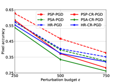
((a)) Pascal VOC

((b)) Cityscapes

((c)) ADE20K

Figure 2: PixAcc after PGD and CR-PGD attacks with $l_{1}$ perturbation vs. perturbation budget $\epsilon$ on the three models and datasets.

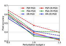
((a)) Pascal VOC

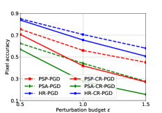
((b)) Cityscapes

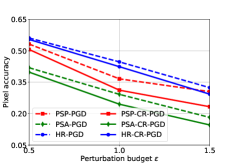
((c)) ADE20K

Figure 3: PixAcc after PGD and CR-PGD attacks with $l_{2}$ perturbation vs. perturbation budget $\epsilon$ on the three models and datasets.

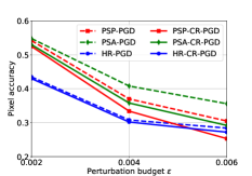
((a)) Pascal VOC

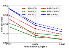
((b)) Cityscapes

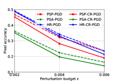
((c)) ADE20K

Figure 4: PixAcc after PGD and CR-PGD attacks with $l_{\infty}$ perturbation vs. perturbation budget $\epsilon$ on the three models and datasets.

Parameter settings. Consider black-box attacks are more challenging than white-box attacks, we set different values for certain hyperparameters in the two attacks. For instance, we set a larger $l_{p}$ perturbation budget $\epsilon$ and larger number of iterations $T$ when evaluating black-box attacks.

• White-box attack settings. Our CR-PGD and PGD attacks share the same hyperparameters. Specifically, we set the total number of iterations $T=50,50,20$ and the learning rate $\alpha=\frac{2.5\epsilon}{T},\frac{2.5\epsilon}{T},\frac{\epsilon}{T}$ to generate $l_{1}$ $l_{2}$, and $l_{\infty}$ perturbations, respectively. We set the weight parameters $a=2$ and $b=-4$, and $\textrm{INT}=M$. We also study the impact of the important hyperparameters in our CR-PGD attack: Gaussian noise $\sigma$ in certified radius, number of samples $M$ in Monte Carlo sampling, and $l_{p}$ perturbation budget $\epsilon$, etc. By default, we set $\sigma=0.001$ and $M=8$, and $\epsilon=750,1.5,0.006$ for $l_{1}$, $l_{2}$, and $l_{\infty}$ perturbations, respectively. When studying the impact of a hyperparameter, we fix the other hyperparameters to be their default values.

• Black-box attack settings. We set the learning rate $\alpha=5\cdot 10^{-4}$, Gaussian noise $\sigma=0.001$, number of samples $M=8$, weight parameters $a=2$ and $b=-4$, and $\textrm{INT}=2M$. We mainly study the impact of the total number of iterations $T$ and the $l_{p}$ perturbation budget $\epsilon$. By default, we set $T=15,000$ and $\epsilon=10000,10,0.05$ for $l_{1}$, $l_{2}$, and $l_{\infty}$ perturbations, respectively.

Evaluation metrics. We use two common metrics to evaluate attack performance to image segmentation models.

• Pixel accuracy (PixAcc): Fraction of pixels predicted correctly by the target model over the testing set.

• Mean Intersection over Union (MIoU): For each testing image $x$ and pixel label $c$, it first computes the ratio $IoU_{c}^{x}=\frac{|P_{c}^{x}\bigcap G_{c}^{x}|}{|P_{c}^{x}\bigcup G_{c}^{x}|}$, where $P_{c}^{x}$ denotes the pixels in $x$ predicted as label $c$ and $G_{c}^{x}$ denotes the pixels in $x$ with the groudtruth label $c$. Then, MIoU is the average of $IoU_{c}^{x}$ over all testing images and all pixel labels.

5.2 Results on White-box Attacks

In this section, we show results on white-box attacks to segmentation models. We first compare the existing attacks and show that the PGD attack achieves the best attack performance. Next, we compare our certified radius-guided PGD attack with the PGD attack. Finally, we study the impact of the important hyperparameters in our CR-PGD attack. We defer all MIoU results to Appendix A.2.

TABLE III: Pixel accuracy with the existing attacks.

Attack	Norm	Dataset
		Pascal VOC	CityScapes	ADE20K
FGSM	$l_{1}$	$79.8\%$	$90.8\%$	$59.4\%$
	$l_{2}$	$80.7\%$	$91.0\%$	$59.9\%$
	$l_{\infty}$	$74.7\%$	$85.1\%$	$54.4\%$
DAG	$l_{\infty}$	$69.1\%$	$75.4\%$	$47.8\%$
PGD	$l_{1}$	$37.7\%$	$63.0\%$	$17.0\%$
	$l_{2}$	$39.7\%$	$58.1\%$	$18.2\%$
	$l_{\infty}$	$30.5\%$	$26.1\%$	$23.5\%$

5.2.1 Verifying that PGD outperforms the existing attacks

We compare the PGD attack [7] with FGSM [7] and DAG [3], two other well-known attacks to image segmentation models (Please see their details in Appendix A.3). Note that DAG is only for $l_{\infty}$ perturbation. We set the perturbation budget $\epsilon$ to be $750,1.5,0.006$ for $l_{1}$, $l_{2}$, and $l_{p}$ perturbations, respectively. The compared results of these attacks are shown in Table III. We observe that PGD consistently and significantly outperforms FGSM and DAG in all the three datasets. Based on this observation, we will select PGD as the default base attack in our certified radius-guided attack framework.

5.2.2 Comparing CR-PGD with PGD

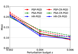
((a)) Pascal VOC

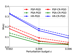
((b)) Cityscapes

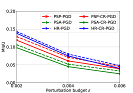
((c)) ADE20K

Figure 14: MIoU after PGD and CR-PGD attacks with $l_{\infty}$ perturbation vs. perturbation budget $\epsilon$ on the three models and datasets

We compare PGD and CR-PGD attacks with respect to $l_{1}$, $l_{2}$, and $l_{\infty}$ perturbations. The pixel accuracy on the three datasets vs. perturbation budget $\epsilon$ are shown in Figure 2, Figure 3, and Figure 4, respectively. The MIoU on the three datasets vs. $l_{1}$, $l_{2}$, and $l_{\infty}$ perturbation budget $\epsilon$ are shown in Figure 12, Figure 13, and Figure 14 in Appendix A.2, respectively. We have the following observations:

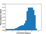
((a)) PGD

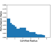
((b)) CR-PGD

Figure 5: Distribution of pixel perturbations vs. pixel-wise certified radius of PGD and CR-PGD on 10 random images.

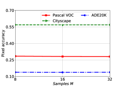
((a)) $L_{1}$ perturbation

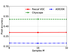
((b)) $L_{2}$ perturbation

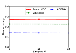
((c)) $L_{\infty}$ perturbation

Figure 6: Impact of the #samples $M$ on our CR-PGD attack with different $l_{p}$ perturbations.

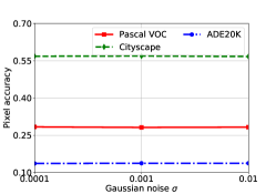
((a)) $L_{1}$ perturbation

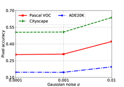
((b)) $L_{2}$ perturbation

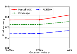
((c)) $L_{\infty}$ perturbation

Figure 7: Impact of the Gaussian noise $\sigma$ on our CR-PGD attack with different $l_{p}$ perturbations.

Our CR-PGD attack consistently outperforms the PGD attack in all datasets, models, and $l_{p}$ perturbations. For instance, when attacking PSANet on Cityscapes with $l_{1}$-perturbation and $\epsilon=500$, our CR-PGD attack has a relative $53.8\%$ gain over the PGD attack in reducing the pixel accuracy; When attacking HRNet on Pascal VOC with $l_{2}$-perturbation and $\epsilon=1.5$, CR-PGD has a relative $9.4\%$ gain over PGD; When attacking PSPNet on ADE20K with $l_{\infty}$-perturbation and $\epsilon=0.004$, CR-PGD has a relative $12.7\%$ gain over PGD. Across all settings, the average relative gain of CR-PGD over PGD is 13.9%.

These results validate that pixel-wise certified radius can indeed guide CR-PGD to find better perturbation directions, and thus help better allocate the pixel perturbations. To further verify it, we aim to show that more perturbations should be added to the pixels that easily affected others, such that more pixels are misclassified. We note that directly finding pixels that mostly easily affect others is a challenging combinatorial optimization problem. Hence we use an alternative way, i.e., show the distribution of pixel perturbations vs. pixel-wise certified radius, to approximately show the effect. Our intuition is that: for pixels with small certified radii, perturbing them can also easily affect other neighboring pixels with small certified radii. This is because neighboring pixels with small certified radii can easily affect each other, which naturally forms the groups in the certified radius map (also see Figure 1(i)). Figure 5 verifies this intuition, where we test 10 random testing images in Pascal VOC. We can see that a majority of the perturbations in CR-PGD are assigned to the pixels with relatively smaller certified radii, in order to wrongly predict more pixels. In contrast, most of the perturbations in PGD are assigned to the pixels with relatively larger certified radii. As wrongly predicting these pixels requires a larger perturbation, PGD misclassifies much fewer pixels than our CR-PGD.

Different models have different robustness. Overall, HRNet is the most robust against the PGD and CR-PGD attacks, in that it has the smallest PixAcc drop when $\epsilon$ increases. On the other hand, PSPNet is the most vulnerable. We note that [7] has similar observations.

Running time comparison. Over all testing images in the three datasets, the average time of CR-PGD is 4.0 seconds, while that of PGD is 3.6 seconds. The overhead of CR-PGD over PGD is 11%.

TABLE IV: PixAcc with different $a$ and $b$ in $l_{2}$ CR-PGD.

Dataset		$b=-2$	$b=-3$	$b=-4$
Pascal VOC	$a=1$	33.6%	35.6%	38.1%
	$a=2$	28.3%	31.8%	30.9%
	$a=3$	32.4%	31.2%	30.7%
CityScape	$a=1$	54.1%	55.3%	56.5%
	$a=2$	52.7%	52.5%	50.7%
	$a=3$	54.8%	53.5%	52.6%
ADE	$a=1$	17.7%	18.6%	20.0%
	$a=2$	15.1%	16.2%	14.6%
	$a=3$	14.4%	15.0%	15.3%

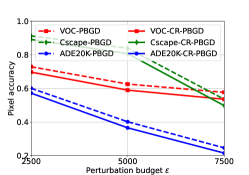
((a)) $l_{1}$ perturbation

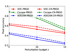
((b)) $l_{2}$ perturbation

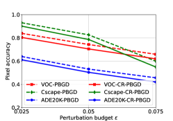
((c)) $l_{\infty}$ perturbation

Figure 8: PixAcc after the black-box PBGD and CR-PBGD attacks with different $l_{p}$ perturbations vs. perturbation budget $\epsilon$.

5.2.3 Impact of the hyperparameters in CR-PGD

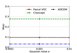
((a)) $l_{1}$ perturbation

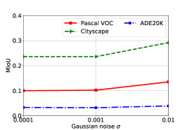
((b)) $l_{2}$ perturbation

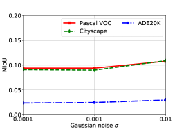
((c)) $l_{\infty}$ perturbation

Figure 16: MIoU: Impact of the Gaussian noise $\sigma$ on our CR-PGD attack with different $l_{p}$ perturbations.

Pixel-wise certified radius and pixel weights are key components in our CR-PGD attack. Here, we study the impact of important hyperparameters in calculating the pixel-wise certified radius: number of samples $M$ in Monte Carlo sampling and Gaussian noise $\sigma$, and $a$ and $b$ in calculating the pixel weights. Figure 6 (and Figure 15 in Appendix) and Figure 7 (and Figure 16 in Appendix) show the impact of $M$ and $\sigma$ on our CR-PGD attack’s pixel accuracy with $l_{1}$, $l_{2}$, and $l_{\infty}$ perturbation, respectively. Table IV shows our CR-PGD attack’s pixel accuracy with different $a$ and $b$. We observe that: (i) Our CR-PGD attack is not sensitive to $M$. The benefit of this is that an attacker can use a relatively small $M$ in order to save the attack time. (ii) Our CR-PGD attack has stable performance within a range of small $\sigma$. Such an observation can guide an attacker to set a relatively small $\sigma$ when performing the CR-PGD attack. More results on studying the impact of $\sigma$ w.r.t. $l_{1},l_{2},l_{\infty}$ perturbations on different models and datasets are shown in Figure  17 to Figure 19 in Appendix A.2. (iii) Our CR-PGD attack is stable across different $a$ and $b$, and $a=2$ and $b=-4$ achieves the best tradeoff.

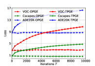
((a)) Attack loss

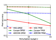
((b)) Attack performance

Figure 9: TPGE vs. OPGE. (a) Attack loss; (b) Attack performance.

5.3 Results on Black-Box Attacks

In this subsection, we show results on black-box attacks. We first compare the gradient estimators proposed in Section 4.3. Then, we compare our proposed PBGD and CR-PBGD attacks. Finally, we study the impact of the number of queries, which is specific to black-box attacks. Note that we do not study the impact of other hyperparameters as our attacks are not sensitive to them, shown in the white-box attacks.

5.3.1 Comparing different gradient estimators

In this experiment, we compare our two-point gradient estimator (TPGE) with the OPGE for simplicity. We do not compare with the deterministic ZOO as it requires very huge number of queries, which is computationally intensive and impractical. We also note that stochastic NES [47] has very close performance as OPGE. For example, with an $l_{2}$ perturbation to be 10, we test on Pascal VOC with the PSPNet model and set #populations to be 100. The PixAcc with NES is 77.4%, which is close to OPGE’s 76.9%. For conciseness, we thus do not show NES’s results. Figure 9 shows the results on attack loss and attack performance. We observe in Figure 9(a) that the attack loss obtained by our TPGE stably increases, while obtained by the OPGE is unstable and sometimes decreases. Moreover, as shown in Figure 9(b), black-box attacks with TPGE achieve much better attack performance than with the OPGE—almost fails to work. The two observations validate that our TPGE outperforms the OPGE in estimating gradients and thus is more useful for attacking image segmentation models.

5.3.2 Comparing PBGD with CR-PBGD

Figure 8 shows the PixAcc with our PBGD and CR-PBGD attacks and different $l_{p}$ perturbations vs. perturbation budget $\epsilon$ on the three models and datasets. The MIoU results are shown in Appendix A.2. We have two observations. First, as $\epsilon$ increases, the PixAcc decreases in all models and datasets with both CR-PBGD and PBGD attacks. Note that the PixAccs are larger that those achieved by white-box attacks (See Figures 2-4). This is because white-box attacks use the exact gradients, while black-box attacks use the estimated ones. Second, CR-PBGD shows better attack performance than PBGD from two aspects: (i) All models have a smaller pixel accuracy with the CR-PBGD attack than that with the PBGD attack. (ii) The CR-PBGD attack can decrease the pixel accuracy more than the PBGD attack as $\epsilon$ increases. These results again demonstrate that the certified radius is beneficial to find more “vulnerable” pixels to be perturbed.

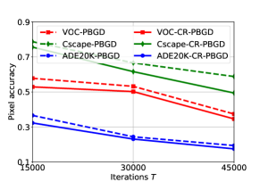
Figure 10: Impact of the iterations $T$ on black-box PBGD and CR-PBGD attacks with $l_{2}$ perturbation on the three datasets.

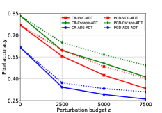
((a)) $l_{1}$ perturbation

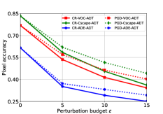
((b)) $l_{2}$ perturbation

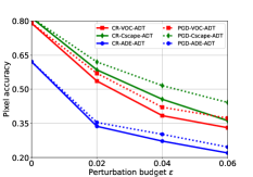
((c)) $l_{\infty}$ perturbation

Figure 11: Defending against white-box PGD and CR-PGD attack via fast adversarial training on the three models and datasets.

5.3.3 Impact of the number of iterations/queries

Note that with $T$ iterations, our CR-PBGD attack has total queries $2.5T$ (with $\textrm{INT}=2M$), while the PBGD attack has total queries $2T$. For a fair comparison, we set a same number of queries for PBGD, i.e., we set its iteration number to be $1.25T$. For brevity, we still use a same notation $T$ when comparing them.

Figure 10 shows the PixACC vs. $T$ against $l_{2}$ perturbation. Note that the results on $l_{1}$ and $l_{\infty}$ perturbations have similar tendency. Figure 21 in Appendix A.2 shows the MIoU vs. $T$. We observe that both the attacks perform better as $T$ increases. This is because a larger number of queries can reveal more information about the segmentation model to the attacker. Compared with PBGD, the CR-PBGD attack can decrease the pixel accuracy faster.

5.4 Defenses

One defense is attempting to remove the certified radius information of all pixels, thus making the certified radius information no longer useful for attackers. However, this method will make the image segmentation model useless. Specifically, remember that a pixel’s certified radius indicates the pixel’s intrinsic confidence to be correctly predicted. To remove certified radius information, we must require the pixel’s outputted confidence scores to be even across all labels, which means the image segmentation models’ performance is random guessing.

A second defense is to design robust image segmentation models using the existing defenses. Particularly, we choose the state-of-the-art empirical defense fast adversarial training (FastADT) [66], and certified defense SEGCERTIFY [67]. To avoid the sense of false security [68], we only defend against the white-box CR-PGD attack. We first compare FastADT and SEGCERTIFY. Note that SEGCERTIFY can only defend against the $l_{2}$ perturbation. By setting an $l_{2}$ perturbation budget as 10, the PixAccs with SEGCERTIFY are 21.9%, 26.3%, and 17.5% on the three datasets, respectively, while those with FastADT are 41.4%, 45.6%, and 29.2%, respectively. These results show that FastADT significantly outperforms SEGCERTIFY. Next, we focus on adopting FastADT to defend against CR-PGD. Figure 11 and Figure 20 in Appendix A.2 show PixAcc and MIoU with FastADT vs. perturbation budget $\epsilon$ on the three models and datasets against CR-PGD, respectively. As a comparison, we also show defense results against the PGD attack. We observe that: (i) FastADT achieves an accuracy-robustness tradeoff, i.e., the clean (undefended) pixel accuracy decreases at the cost of maintaining the robust accuracy against the attacks. (ii) CR-PGD is more effective than PGD against FastADT, which again verified that pixel-wise certified radius is important to design better attacks.

A third defense is to enhance the existing strongest defenses, i.e., FastADT. The current FastADT is trained on adversarial perturbations generated by the state-of-the-art PGD attack and then used to defend against our CR-PGD attack. Here, we propose a variant of FastADT, called CR-FastADT, which assumes the defender knows the details of our CR-PGD attack, and trains on adversarial perturbations generated by our CR-PGD. For instance, we evaluate CR-FastADT on Pascal VOC with PSPNet. When setting the $L_{2}$ perturbation to be 5, 10, 15, the PixAccs with CR-FastADT are 59.8%, 47.9%, and 38.7% respectively, which are marginally (1.3%, 2.3%, and 2.5%) higher than those with FastADT, i.e., 58.5%, 45.6%, and 36.2%. This verifies that CR-FastADT is a slightly better defense than FastADT, but not that much.

TABLE V: Comparing FGSM and CR-FGSM.

Model	FGSM			CR-FGSM
	$l_{1}$	$l_{2}$	$l_{\infty}$	$l_{1}$	$l_{2}$	$l_{\infty}$
PSPNet-Pascal	$79.8\%$	$80.7\%$	$74.7\%$	$78.7\%$	$79.1\%$	$73.2\%$
HRNet-Cityscape	$37.7\%$	$63.0\%$	$17.0\%$	$36.1\%$	$61.6\%$	$15.6\%$
PSANet-ADE20K	$59.4\%$	$59.9\%$	$54.4\%$	$57.9\%$	$58.6\%$	$53.4\%$

6 Discussion

Applying our certified radius-guided attack framework to other attacks. In the paper, we mainly apply the pixel-wise certified radius in the PGD attack. Actually, it can be also applied in other attacks such as the FGSM attack [7] (Details are shown in the Appendix A.3) and enhance its attack performance as well. For instance, Table V shows the pixel accuracy with FGSM and FGSM with certified radius (CR-FGSM) on the three image segmentation models and datasets. We set all parameters same as PGD/CR-PGD. For instance, the perturbation budget $\epsilon$ is $\epsilon=750,1.5,0.006$ for $l_{1}$, $l_{2}$, and $l_{\infty}$ perturbations, respectively. We observe that CR-FGSM consistently produces a lower pixel accuracy than FGSM in all cases, showing that certified radius can also guide FGSM to achieve better attack performance.

Randomized smoothing vs. approximate local Lipschitz based certified radius. Weng et al. [69] proposed CLEVER, which uses sampling to estimate the local Lipschitz constant, then derives the certified radius for image classification models. CLEVER has two sampling relevant hyperparameters $N_{b}$ and $N_{s}$. In the untargeted attack case (same as our setting), CLEVER requires sampling the model $N_{b}\times N_{s}\times|\mathcal{Y}|$ times to derive the certified radius, where $|\mathcal{Y}|$ is the number of classes. The default value of $N_{b}$ and $N_{s}$ are 50 and 1024, respectively. We can also adapt CLEVER to derive pixel’s certified radius for segmentation models and use it to guide PGD attack.

With these defaults values, we test that CLEVER is 4 orders of magnitude slower than randomized smoothing. We then reduce $N_{b}$ and $N_{s}$. When $N_{b}=10$ and $N_{s}=32$, CLEVER is 2 orders of magnitude slower, and its attack effectiveness is less effective than ours. E.g., on Pascal VOC dataset and PSPNet model, with $l_{2}$ perturbation budget $1.5$, it achieves an attack accuracy $35.4\%$, while our CR-PGD attack achieves $30.9\%$. In the extreme case, we set $N_{b}=10$ and $N_{s}=1$ and CLEVER is still 1 order of magnitude slower, and it only achieves $41.6\%$ attack accuracy, even worse than vanilla PGD attack which achieves $39.7\%$. This is because the calculated pixels’ certified radii are very inaccurate when $N_{s}=1$.

Evaluating our attack framework for target attacks. Our attack framework is mainly for untargeted attacks, i.e., it aims to misclassify as many pixels as possible, while not requiring what wrong labels to be. This is actually due to the inherent properties of certified radius—if a pixel has a small certified radius, this pixel is easily misclassified to be any wrong label, but not a specific one. On the other hand, targeted attacks misclassify pixels to be specific wrong labels. Nevertheless, we can still adapt our attack framework to perform the targeted attack, where we replace the existing attack loss for untargeted attacks to be that for target attacks. We experiment on Pascal VOC and PSPNet with a random target label and 500 testing images and set $l_{2}$ perturbation budget as 10. We show that 95.3% of pixels are misclassified to be the target label using our adapted attack, and 96.5% of pixels are misclassified to be the target label using the state-of-the-art target attack [81]. This result means our attack is still effective and achieves comparable results with specially designed targeted attacks.

Comparing white-box CR-PGD vs. black-box CR-BPGD. We directly compare our white-box CR-PGD and black-box CR-BPGD in the same setting, and consider $l_{2}$ perturbation. Specifically, by setting the perturbation budget $\epsilon=5,10,15$, pixel accuracies with CR-PGD are 17.9%, 13.7%, and 10.4%, respectively, while that with CR-BPGD are 61.7%, 52.9%, and 45.5%, respectively. The results show that white-box attacks are much more effective than black-box attacks and thus there is still room to improve the performance of black-box attacks.

Adversarial training with CR-PGD samples. We evaluate CR-PGD for adversarial training and recalculate the CR for the pixels with the (e.g., 20%) least CR. Using CR-PGD for adversarial training increases the CR of these pixels by 11%. This shows that CR-PGD can also increase the robustness of “easily perturbed” pixels.

Defending against black-box attacks. We use FastADT to defend against our black-box CR-PBGD attack. We evaluate FastADT on Pascal VOC with the PSPNet model and set $l_{2}$ perturbation to be 10. We note that the PixAcc with no defense is 52.9%, but can be largely increased to 71.5% when applying FastADT. As emphasized, a defender cares more on defending against the “strongest” white-box attack, as defending against the “weakest” black-box attack does not mean the defense is effective enough in practice. This is because an attacker can always leverage better techniques to enhance the attack.

Applying our attacks in the real world and the difficulty. Let’s consider tumor detection and traffic sign prediction systems. An insider in an insurance company can be a white-box attacker, i.e., s/he knows the tumor detection algorithm details. S/He can then modify her/his medical images to attack the algorithm offline by using our white-box attack and submitting modified images for fraud insurance claims. An outsider that uses a deployed traffic sign prediction system can be a black-box attacker. For example, s/he can iteratively query the system with perturbed “STOP” sign images and optimize the perturbation via our black-box attacks. The attack ends when the final perturbed “STOP” sign is classified, e.g., as a “SPEED” sign. S/He finally prints this perturbed “STOP” sign for physical-world attacks. The difficulties lie in that this attack may involve many queries, but note that there indeed exist physical-world attacks using the perturbed “STOP” sign [82].

7 Related Work

Attacks. A few white-box attacks [3, 4, 6, 7] have been proposed on image segmentation models. For instance, Xie et al. [3] proposed the first gradient based attack to segmentation models. Motivated by that pixels are separately classified in image segmentation, they developed the Dense Adversary Generation (DAG) attack that considers all pixels together and optimizes the summation of all pixels’ losses to generate adversarial perturbations. Arnab et al. [7] presented the first systematic evaluation of adversarial perturbations on modern image segmentation models. They adopted the FGSM [11, 12] and PGD [13] as the baseline attack. Existing black-box attacks, e.g., NES [47], SimBA [55] and ZOO [54], to image classification models can be adapted to attack image segmentation models. However, they are very query inefficient.

Defenses. A few defenses [83, 84, 85, 86, 87, 67] have been proposed recently to improve the robustness of segmentation models against adversarial perturbations. For instance, Xiao et al. [83] first characterized adversarial perturbations based on spatial context information in segmentation models and then proposed to detect adversarial regions using spatial consistency information. Xu et al. [87] proposed a dynamic divide-and-conquer adversarial training method. Latterly, Fischer et al. [67] adopted randomized smoothing to develop the first certified segmentation. Note that we also use randomized smoothing in this paper, but our goal is not to use it to defend against attacks.

Certified radius. Various methods [14, 15, 16, 17, 18, 19, 20, 21, 22, 23, 24, 25, 26, 27, 28, 29, 30] have been proposed to derive the certified radius for image classification models against adversarial perturbations. However, these methods are not scalable. Randomized smoothing [31, 32, 33, 34, 35, 36, 37, 38, 39, 40, 41, 42, 43, 44, 45] was the first method to certify the robustness of large models and achieved the state-of-the-art certified radius. For instance, Cohen et al. [33] obtained a tight $l_{2}$ certified radius with Gaussian noise on normally trained image classification models. Salman et al. [46] improved [33] by combining the design of an adaptive attack against smoothed soft image classifiers and adversarial training on the attacked classifiers. Many follow-up works [43, 88, 89, 42, 41, 90, 91] extended randomized smoothing in various ways and applications. For instance, Fischer et al. [89] and Li et al. [88] proposed to certify the robustness against geometric perturbations. Chiang et al. [91] introduced median smoothing and applied it to certify object detectors. Jia et al. [41] and Wang et al. [42] applied randomized smoothing in the graph domain and derived the certified radius for community detection, node/graph classifications methods against graph structure perturbation.

In contrast, we propose to leverage certified radius derived by randomized smoothing to design better attacks against image segmentation models.

8 Conclusion

We study attacks to image segmentation models. Compared with image classification models, image segmentation models have richer information (e.g., predictions on each pixel instead of on an whole image) that can be exploited by attackers. We propose to leverage certified radius, the first work that uses it from the attacker perspective, and derive the pixel-wise certified radius based on randomized smoothing. Based on it, we design a certified radius-guide attack framework for both white-box and black-box attacks. Our framework can be seamlessly incorporated into any existing attacks to design more effective attacks. Under black-box attacks, we also design a random-free gradient estimator based on bandit: it is query-efficient, unbiased and stable. We use our gradient estimator to instantiate PBGD and certified radius-guided PBGD attacks, both with a tight sublinear regret bound. Extensive evaluations verify the effectiveness and generalizability of our certified radius-guided attack framework.

Acknowledgments. We thank the anonymous reviewers for their constructive feedback. This work was supported by Wang’s startup funding, Cisco Research Award, and National Science Foundation under grant No. 2216926.

Appendix A Appendices

Input: Image segmentation model $F_{\theta}$, testing image $x$ with pixel labels $y$, perturbation budget $\epsilon$, learning rate $\alpha$, #iterations $T$, weight parameters $a$ and $b$, #samples $M$, Gaussian variance $\sigma$, interval INT.

Output: Adversarial perturbation $\delta^{(T)}$.

1 Initialize: $\delta^{(0)}=0\in\mathbb{B}=\{\delta:\|\delta\|_{p}\leq\epsilon\}$.

2 for $t=0,1,\cdots,T-1$ do

3       if t mod INT != 0 then

4             Reuse the pixel weights:

5      else

6             Sample $M$ noises: $\beta_{j}\sim\mathcal{N}(0,\sigma^{2}I),j\in\{1,2,...,M\}$;

7             Define the perturbed image: $x^{(t)}=x+\delta^{(t)}$;

8             Compute the smoothed segmentation model: $G(x^{(t)})=\frac{1}{M}\sum_{j=1}^{M}F_{\theta}(x^{(t)}+\beta_{j})$;

9             Estimate the lower bound probabilities of the top label for each pixel $x^{(t)}_{n}$: $\underline{p_{n}}=\max_{c}{G(x^{(t)})_{n,c}}$;

10             Calculate the certified radius for each pixel $x^{(t)}_{n}$: $cr(x^{(t)}_{n})=\sigma\Phi^{-1}(\underline{p_{n}})$;

11             Assign a weight to each pixel $x^{(t)}_{n}$:

12       end if

13      

14      Define the certified radius-guided loss: $L_{cr}(F_{\theta}(x^{(t)}),y)=\frac{1}{N}\sum_{n=1}^{N}w^{(t)}_{n}\cdot L(F_{\theta}(x_{n}^{(t)}),y_{n})$;

15       Run CR-PGD to update the adversarial perturbation: $\delta^{(t+1)}=\textrm{Proj}_{\mathbb{B}}(\delta^{(t)}+\alpha\cdot\nabla_{\delta^{(t)}}L_{\textrm{cr}}(F_{\theta}(x^{(t)}),y))$.

16 end for

return $\delta^{(T)}$

Algorithm 1 Certified radius-guided white-box PGD attacks to image segmentation models

Input: Image segmentation model $F_{\theta}$, testing image $x$ with pixel labels $y$, perturbation budget $\epsilon$, learning rate $\alpha$, parameter $\gamma$, #iters $T$, weight parameters $a$ and $b$, #samples $M$, Gaussian variance $\sigma$, CRFlag, interval INT.

Output: Adversarial perturbation $\delta^{(T)}$.

1 Initialize: $\delta^{(0)}=0\in\mathbb{B}=\{\delta:\|\delta\|_{p}\leq\epsilon\}$.

2 for $t=0,1,\cdots,T-1$ do

3       Sample a unit vector $\bm{u}^{(t)}\in\mathbb{S}_{p}$ uniformly at random;

4       Query $F_{\theta}$ twice to obtain predictions: $p_{1}=F_{\theta}(x+\delta^{(t)}+\gamma\bm{u}^{(t)})$ and $p_{2}=F_{\theta}(x+\delta^{(t)}-\gamma\bm{u}^{(t)})$;

5      

6      if  (CRFlag == false)  then

7             /*PBGD: Without pixel-wise certified radius*/

8             Obtain the loss feedback:

9             $\ell_{1}=L(p_{1},y)$ and $\ell_{2}=L(p_{2},y)$;

10            Estimate the gradient: $\tilde{g}=\frac{N}{2\gamma}\big{(}\ell_{1}-\ell_{2}\big{)}\bm{u}^{(t)}$;

11            Run PBGD to update the adversarial perturbation: $\delta^{(t+1)}=\textrm{Proj}_{\mathbb{B}}(\delta^{(t)}+\alpha\cdot\tilde{g})$.

12      else

13             /*CR-PBGD: With pixel-wise certified radius*/

14            

15            Calculate the pixel-wise certified radius and define $L_{cr}$ using $F_{\theta},a,b,M,\sigma,t$ as in Algorithm 1;

16            Obtain the certified radius-guided loss feedback:

17             $\ell_{cr,1}=L_{cr}(p_{1},y)$ and $\ell_{cr,2}=L_{cr}(p_{2},y)$;

18            Estimate the gradient: $\tilde{g}_{cr}=\frac{N}{2\gamma}\big{(}\ell_{cr,1}-\ell_{cr_{2}}\big{)}\bm{u}^{(t)}$;

19            Run CR-PBGD to update the adversarial perturbation: $\delta^{(t+1)}=\textrm{Proj}_{\mathbb{B}}(\delta^{(t)}+\alpha\cdot\tilde{g}_{cr})$.

20       end if

21      

22 end for

return $\delta^{(T)}$

Algorithm 2 Black-box PBGD and CR-PBGD to image segmentation models

Input: Segmentation model $F_{\theta}$, testing image $x$ with label $y$, #epochs $T$, perturbation budget $\epsilon$.

Output: Adversarial perturbation $\delta$.

1 Initialize: $x^{(1)}\leftarrow x$, $\delta^{(0)}=0$.

2 for $t=1,2,\cdots,T$ do

3      

4      $\delta^{(t)}\leftarrow\nabla_{\delta^{(t)}}F_{\theta}(x^{(t)}+\delta^{(t-1)},y)-\nabla_{\delta^{(t)}}F_{\theta}(x^{(t)},y)$

5      

6      $\delta^{(t)}=\frac{0.5\delta^{(t)}}{||\delta^{(t)}||_{\infty}}$

7      

8      $\delta=\textrm{Clip}(\delta+\delta^{(t)},\epsilon)$

9       $x^{(t+1)}=x^{(t)}+\delta^{(t)}$

10      

11 end for

return $\delta$

Algorithm 3 DAG for $l_{\infty}$ perturbation

A.1 Dataset Details

Detailed of the used datasets are as below:

• Pascal VOC [63]. It consists of internet images labeled with 21 different classes. The training set has 10582 images when combined with additional annotations from  [93]. The validation set contains 1449 images.

• Cityscapes [64]. It consists of road-scenes captured from car-mounted cameras and has 19 classes. The training set totals 2975 images and the validation set has 500 images. As the dataset contains high-resolution images (2048×1024 pixels) that require too much memory for segmentation models, we resize all images to 1024x512 before training, same as [7].

• ADE20K [65]. It is a densely annotated image dataset that covers 365 scenes and 150 object categories with pixel-wise annotations for scene understanding. The dataset contains 27,574 images, where 25,574 images form the training set and the remaining 2,000 images as the testing set.

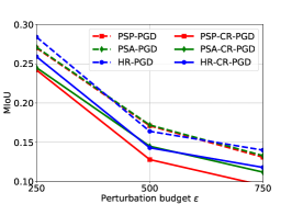
((a)) Pascal VOC

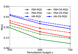
((b)) Cityscapes

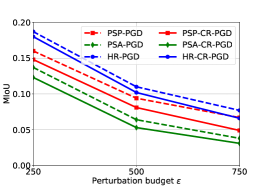
((c)) ADE20K

Figure 12: MIoU after PGD and CR-PGD attacks with $l_{1}$ perturbation vs. perturbation budget $\epsilon$ on the three models and datasets

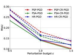
((a)) Pascal VOC

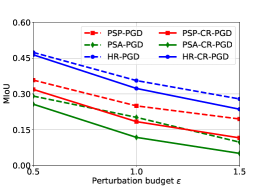
((b)) Cityscapes

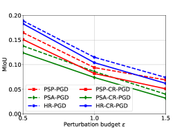
((c)) ADE20K

Figure 13: MIoU after PGD and CR-PGD attacks with $l_{2}$ perturbation vs. perturbation budget $\epsilon$ on the three models and datasets

A.2 More Experimental Results

MIoU after PGD and CR-PGD attacks. See Figures 12, 13, and  14 for $l_{1}$, $l_{2}$, and $l_{\infty}$ perturbations, respectively. We can observe that our CR-PGD outperforms PGD.

Impact of $M$ and $\sigma$ on MIoU. See Figures 15 and 16, respectively. We see that CR-PGD is insensitive to $M$ and a relatively larger $\sigma$ will negatively impact our CR-PGD.

Impact of $\sigma$ on more datasets and models. See Figures 17-19. We see that CR-PGD is insensitive to $\sigma$ within a range.

Defense results on MIoU. See Figure 20 the defense results of FastADT on MIoU against CR-PGD with different $l_{p}$ perturbations.

Black-box attack results on MIoU. See Figure 21 the impact of iterations/queries on MIoU with our PBGD and CR-PBGD black-box attacks and the $l_{2}$ perturbation on the three datasets.

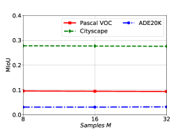
((a)) $l_{1}$ perturbation

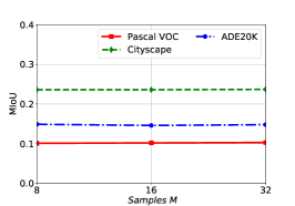
((b)) $l_{2}$ perturbation

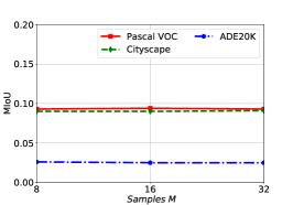
((c)) $l_{\infty}$ perturbation

Figure 15: MIoU: Impact of the #samples $M$ on our CR-PGD attack with different $l_{p}$ perturbations.

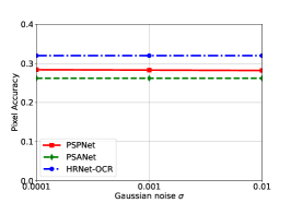
((a)) Pascal VOC

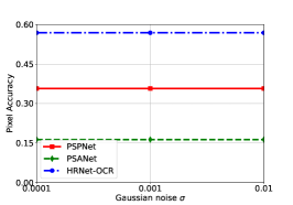
((b)) Cityscape

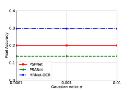
((c)) ADE20K

Figure 17: Impact of the Gaussian noise $\sigma$ on our CR-PGD attack with different datasets and models, under $l_{1}$ perturbation.

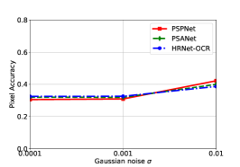
((a)) Pascal VOC

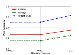
((b)) Cityscape

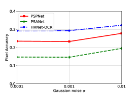
((c)) ADE20K

Figure 18: Impact of the Gaussian noise $\sigma$ on our CR-PGD attack with different datasets and models, under $l_{2}$ perturbation.

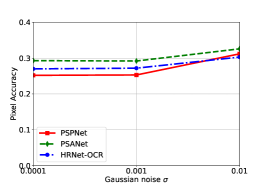
((a)) Pascal VOC

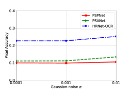
((b)) Cityscape

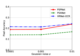
((c)) ADE20K

Figure 19: Impact of the Gaussian noise $\sigma$ on our CR-PGD attack with different datasets and models, under $l_{\infty}$ perturbation.

A.3 Attacks and Defense

We first briefly introduce the Fast Gradient Sign Method (FGSM) [11], Projected Gradient Descent (PGD) [13], and Dense Adversary Generation (DAG) [3] attacks. Then, we introduce the fast adversarial training (FastADT) defense [66].

Suppose we are given a segmentation model $F_{\theta}$, a loss function $L$, and a testing image $x$ with groudtruth segmentation labels $y$, and the perturbation budget $\epsilon$.

Projected Gradient Descent (PGD). PGD iteratively finds the $l_{p}$ perturbations by increasing the loss of the model on a testing image $x$:

$$\delta\leftarrow\textrm{Proj}_{\mathbb{B}}(\delta+\alpha\cdot\nabla L(F_{\theta}(x+\delta),y)),$$ (21)

where $\alpha$ is the learning rate in PGD and $\mathbb{B}=\{\delta:||\delta||_{p}\leq\epsilon\}$ is the allowable perturbation set. $\textrm{Proj}_{\mathbb{B}}$ projects the adversarial perturbation to the allowable set $\mathbb{B}$. The specific forms of $l_{1}$, $l_{2}$, and $l_{\infty}$ perturbations are as follows:

$$L_{1}:\delta\leftarrow\textrm{Clip}(\delta+\alpha\cdot\frac{\nabla L(F_{\theta}(x+\delta),y)}{||\nabla L(F_{\theta}(x+\delta),y)||_{1}})$$ (22)

$$L_{2}:\delta\leftarrow\textrm{Clip}(\delta+\alpha\cdot\frac{\nabla L(F_{\theta}(x+\delta),y)}{||\nabla L(F_{\theta}(x+\delta),y)||_{2}})$$ (23)

$$L_{\infty}:\delta\leftarrow\textrm{Clip}(\delta+\alpha\cdot\textrm{sign}(\nabla L(F_{\theta}(x+\delta),y),\epsilon),$$ (24)

where $\textrm{Clip}(a,\epsilon)$ makes each $a_{n}$ in the range $[-\epsilon,\epsilon]$.

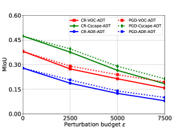
((a)) $l_{1}$ perturbation

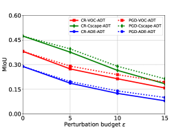
((b)) $l_{2}$ perturbation

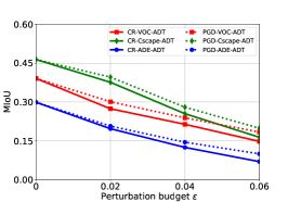
((c)) $l_{\infty}$ perturbation

Figure 20: MIoU: Defending against our white-box CR-PGD attack via fast adversarial training.

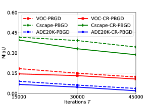
Figure 21: MIoU: PGD and CR-PGD attacks with $l_{2}$ perturbation vs. $T$.

Fast Gradient Sign (FGSM). FGSM is a variant of PGD, where it generates $l_{p}$ perturbations with a single step.

Dense Adversary Generation (DAG). DAG generates an $l_{\infty}$ perturbation to make the predictions of all pixels be wrong (see Algorithm 3 for the details). The perturbation $\delta$ is iteratively generated as follows:

$$\footnotesize\delta\leftarrow\nabla_{\delta}L(F_{\theta}(x+\delta,y))-\nabla_{\delta}L(F_{\theta}(x,y)),\,\delta^{\prime}=\frac{0.5\delta}{||\delta||_{\infty}}.$$ (25)

Algorithm 3 shows the details of DAG.

Input: Segmentation model $F_{\theta}$, perturbation budget $\epsilon$, learning rate $\alpha$, #epochs $T$, a training set $\mathbb{D}_{tr}$.

Output: Model parameters $\theta$.

1 Initialize: $\delta^{(0)}=0\in\mathbb{B}=\{\delta:\|\delta\|_{p}\leq\epsilon\}$.

2 for $t=1,2,\cdots,T$ do

3       for $(x,y)\in\mathbb{D}_{tr}$ do

4             // Perform FGSM adversarial attack

5             $\delta=\textrm{Uniform}(-\epsilon,\epsilon)$

6            

7            $\delta=\textrm{Clip}(\delta+\alpha\cdot\textrm{sign}(\nabla_{\delta}L(F_{\theta}(x+\delta),y)))$

8            

9            // Update model parameters using, e.g., SGD

10            

11            $\theta=\theta-\nabla_{\theta}L(F_{\theta}(x+\delta),y)$

12            

13       end for

14      

15 end for

return $\theta$

Algorithm 4 FastADT: FGSM adv. training

Fast Adversarial Training (FastADT). FastADT aims to speeds up PGD-based adversarial training (AT) [13]. It combines FGSM-based AT with random initialization. Though simple and efficient, it shows comparable defense performance with PGD-based AT. Algorithm 4 illustrates the FastADT.

Definition 2 (Lipschitz continuous).

A real-valued function $f(\cdot)$ is $C$-Lipschitz continuous with respect to $l_{p}$ norm, if, for any two inputs $z_{1}$ and $z_{2}$,

$$|f(z_{1})-f(z_{2})|\leq{C}||z_{1}-z_{2}||_{p}.$$ (26)

Definition 3 (Convex function).

A real-valued function $f(\cdot)$ is convex if and only if the following inequality hold for any two inputs $z_{1}$ and $z_{2}$ in domain and $\rho\in(0,1)$,

$$f(\rho z_{1}+(1-\rho)z_{2})\leq\rho f(z_{1})+(1-\rho)f(z_{2}).$$ (27)

Lemma 1 ([46]).

For any measurable function $g:\mathbb{R}^{N}\to[0,1]$, defining $\hat{g}(x)={E_{\varepsilon\sim N(0,{\sigma^{2}})}}g(x+\varepsilon)$, then $x\mapsto{\Phi^{-1}}(\hat{g}(x))$ is $1/\sigma$-Lipschitz, where $\Phi^{-1}$ is the inverse of the standard Gaussian CDF.

A.4 Proof of Theorem 1

Proof.

Our proof is based on Lemma 1 and Definition 2.

Given a testing image $x$ with pixel labels $y$. For each pixel $x_{n}$, $F_{\theta}(x)_{n,c}$ is the model’s probability of predicting label $c$ on $x_{n}$, and it satisfies $F_{\theta}{(x)_{n,c}}:x\to[0,1]$. From the definition of the smoothed model $G_{\theta}$ of $F_{\theta}$, we have $G_{\theta}{(x)_{n,c}}={E_{\beta\sim N(0,{\sigma^{2}})}}F_{\theta}{(x+\beta)_{n,c}}$. Let $y_{n}=\max_{c}G_{\theta}{(x)_{n,c}}$ and $y^{\prime}_{n}=\max_{c\neq y_{n}}G_{\theta}{(x)_{n,c}}$. Using Lemma 1, we know $x\mapsto{\Phi^{-1}}(G_{\theta}{(x)_{n,c}})$ is $1/\sigma$-Lipschitz. Then, for any pixel perturbation $||\delta||_{2}$, we have

$${\Phi^{-1}}(G_{\theta}{(x+\delta)_{{n,y_{n}}}})>{\Phi^{-1}}(G_{\theta}{(x)_{{n,y_{n}}}})-\frac{1}{\sigma}||\delta||_{2}.$$ (28)

$${\Phi^{-1}}(G_{\theta}{(x)_{n,y^{\prime}_{n}}})+\frac{1}{\sigma}||\delta||_{2}>{\Phi^{-1}}(G_{\theta}{(x+\delta)_{n,y^{\prime}_{n}}}).$$ (29)

To guarantee that the perturbed pixel $(x+\delta)_{n}$ is also correctly predicted, i.e., $y_{n}=\arg\max_{c}G_{\theta}(x+\delta)_{n,c}$, we need that for any perturbation $\delta$,

$$\small{\Phi^{-1}}(G_{\theta}{(x+\delta)_{{n,y_{n}}}})>{\Phi^{-1}}(G_{\theta}{(x+\delta)_{n,y^{\prime}_{n}}}).$$ (30)

In other words, we require

$${\Phi^{-1}}(G_{\theta}{(x)_{{n,y_{n}}}})-\frac{1}{\sigma}||\delta||_{2}>{\Phi^{-1}}(G_{\theta}{(x)_{n,y^{\prime}_{n}}})+\frac{1}{\sigma}||\delta||_{2},$$ (31)

which implies

$$\small||\delta||_{2}<\frac{\sigma}{2}(\Phi^{-1}(G_{\theta}{(x)_{{n,y_{n}}}})-\Phi^{-1}(G_{\theta}{(x)_{n,y^{\prime}_{n}}})).$$ (32)

According the Definition 1, we then have the pixel-wise $l_{2}$ certified radius as follows:

$$cr(x_{n})=\max{\|\delta\|_{2}}=\frac{\sigma}{2}(\Phi^{-1}(G_{\theta}{(x)_{{n,y_{n}}}})-\Phi^{-1}(G_{\theta}{(x)_{n,y^{\prime}_{n}}})).$$

Note that $G_{\theta}{(x)_{n,y^{\prime}_{n}}}\leq 1-G_{\theta}{(x)_{{n,y_{n}}}}$ and $\Phi^{-1}$ is an increasing function. By setting $G_{\theta}{(x)_{n,y^{\prime}_{n}}}=1-G_{\theta}{(x)_{{n,y_{n}}}}$, we have

$$cr(x_{n})=\sigma\Phi^{-1}(G_{\theta}{(x)_{n,y_{n}})}.$$ (33)

∎

A.5 Proof of Theorem 2

Proof.

We first prove that $\hat{g}^{TPGE}$ is an unbiased estimator of $\nabla\hat{L}(\delta)$. The proof that $\hat{g}_{cr}^{TPGE}$ is an unbiased estimator of $\nabla\hat{L}_{cr}(\delta)$ is similar. Recall that $\hat{g}^{TPGE}=\frac{N}{2\gamma}\big{(}L(\delta+\gamma\hat{u})-L(\delta-\gamma\hat{u})\big{)}\hat{u}$ for a sampled $\hat{u}\in\mathcal{S}_{p}$. According to Equation 15, we have the following two equations for directions $\bm{u}$ and $-\bm{u}$,

$$\nabla\hat{L}(\delta)=\mathbb{E}_{\bm{u}\in\mathcal{S}_{p}}[\frac{N}{\gamma}L(\delta+\gamma\bm{u})\bm{u}],$$ (34)

$$\nabla\hat{L}(\delta)=-\mathbb{E}_{\bm{u}\in\mathcal{S}_{p}}[\frac{N}{\gamma}L(\delta-\gamma\bm{u})\bm{u}].$$ (35)

Combining the two equations and rearranging terms, we have $\nabla\hat{L}(\delta)=\mathbb{E}_{\bm{u}\in\mathcal{S}_{p}}[\frac{N}{2\gamma}\big{(}L(\delta+\gamma\bm{u})-L(\delta-\gamma\bm{u})\big{)}\bm{u}]$. Thus, we have $\nabla\hat{L}(\delta)=\mathbb{E}_{\hat{u}}[\hat{g}^{TPGE}]$, proving the unbiasedness of $\hat{g}^{TPGE}$.

Second, we show that $\hat{g}^{TPGE}$ has a bounded norm. The proof that $\hat{g}_{cr}^{TPGE}$ has a bounded norm is similar. As $L(\cdot)$ is $\hat{C}$-Lipschitz continuous (See Definition 2) with respect to $l_{p}$ norm, we have $|L(\delta_{1})-L(\delta_{2})|\leq\hat{C}||\delta_{1}-\delta_{2}||_{p}.$ Then,

$$\footnotesize\begin{split}||\hat{g}^{TPGE}||_{p}&=||\frac{N}{2\gamma}\big{(}L(\delta+\gamma\bm{u})-L(\delta-\gamma\bm{u})\big{)}\bm{u}||_{p}\\ &=\frac{N}{2\gamma}|L(\delta+\gamma\bm{u})-L(\delta-\gamma\bm{u})|\cdot||\bm{u}||_{p}\\ &\stackrel{{\scriptstyle(a)}}{{=}}\frac{N}{2\gamma}|L(\delta+\gamma\bm{u})-L(\delta-\gamma\bm{u})|\\ &\stackrel{{\scriptstyle(b)}}{{\leq}}\frac{N}{2\gamma}\hat{C}||(\delta+\gamma\bm{u})-(\delta-\gamma\bm{u})||_{p}\\ &=\frac{N}{2\gamma}\hat{C}||2\gamma\bm{u}||_{p}=N\hat{C},\end{split}$$ (36)

where (a) is due to that $u$ is a random unit vector and (b) is due to the Lipschitz continuity of $L$. ∎

A.6 Proof of Theorem 3

Proof.

Before analyzing the regret bound of our proposed PBGD and CR-PBGD black-box attack, we first show the regret bound in the white-box setting where the Lipschitz continuous and convex loss function is revealed to the attacker such that the gradient can be exactly derived. Specifically, Zinkevich [79] shows that the regret bound is $\mathcal{O}(\sqrt{T})$ using online projected gradient descent. When using the stochastic gradient whose expectation is equal to the true gradient, the online projected gradient descent still achieves an $\mathcal{O}(\sqrt{T})$ regret bound, which is presented in the following theorem:

Theorem 4 ([79]).

For a $\tilde{C}$-Lipschitz convex loss function $L$ and letting $\tilde{g}^{(t)}$ be the stochastic gradient in round $t$ satisfying $\mathbb{E}[\tilde{g}^{(t)}]=\nabla L$ and $||\tilde{g}^{(t)}||\leq\tilde{C}$. By setting a learning rate $\alpha=\frac{\sqrt{N}}{2\tilde{C}\sqrt{T}}$ in the online projected gradient descent for any total iteration $T>0$, then the regret incurred by the online projected gradient descent is no more than $\sqrt{N}\tilde{C}\sqrt{T}/2$, i.e.,

$$\small\mathbb{E}\{\sum_{t=1}^{T}L(\delta^{(t)})\}-\max_{\delta}\sum_{t=1}^{T}L(\delta)\leq\sqrt{N}\tilde{C}\sqrt{T}/2=\mathcal{O}(\sqrt{T}),$$ (37)

where $\delta^{(t)}=\textrm{Proj}_{\mathbb{B}}(\delta^{(t-1)}+\lambda\tilde{g}^{(t)})$.

Next, we derive the regret bound for PBGD for simplicity and the proof for CR-PBGD is similar. Note that PBGD performs the exact gradient descent on the smoothed function $\hat{L}$ because $\hat{g}^{TPGE}$ is an unbiased gradient estimator of $\nabla\hat{L}$. Based on Theorem 2, we have $||\hat{g}||_{p}\leq N\hat{C}$. From Theorem 4, we can bound the expected regret on $\hat{L}(\delta)$ as follows,

$$\sum_{t=1}^{T}\mathbb{E}[\hat{L}(\delta^{(t)})]-\max_{\delta}\sum_{t=1}^{T}\hat{L}(\delta)\leq N^{3/2}\hat{C}\sqrt{T}/2.$$ (38)

According to the definition of $\hat{L}(\delta)$ in Equation 14, we can bound the difference between $\hat{L}(\delta)$ and $L(\delta)$ as,

$$\small\begin{split}|\hat{L}(\delta)-L(\delta)|&\stackrel{{\scriptstyle(a)}}{{=}}|\mathbb{E}_{\bm{v}\in\mathcal{B}_{p}}[L(\delta+\gamma\bm{v})]-L(\delta)|\\ &=\mathbb{E}_{\bm{v}\in\mathcal{B}_{p}}[|L(\delta+\gamma\bm{v})-L(\delta)|]\\ &\stackrel{{\scriptstyle(b)}}{{\leq}}\mathbb{E}_{\bm{v}\in\mathcal{B}_{p}}[\hat{C}||\gamma\bm{v}||_{p}]=\hat{C}\gamma,\end{split}$$ (39)

where (a) is due to the definition of $\hat{L}$ and (b) is due to the Lipschitz continuity of the loss function $L$.

Then, we can bound $|\hat{L}(\delta^{(t)})-L(\delta)|$ as follows:

$$\small\begin{split}|\hat{L}(\delta^{(t)})-L(\delta)|&=|\hat{L}(\delta^{(t)})-L(\delta^{(t)})+L(\delta^{(t)})-L(\delta)|\\ &\leq|\hat{L}(\delta^{(t)})-L(\delta^{(t)})|+|L(\delta^{(t)})-L(\delta)|\\ &\stackrel{{\scriptstyle(a)}}{{\leq}}\hat{C}\gamma+\hat{C}\gamma=2\hat{C}\gamma,\end{split}$$ (40)

where we apply Equation 39 to the first term and the Lipschitz continuity of attack loss $L(\delta)$ for the second term.

With the above inequality, we can obtain the lower bound of Equation 38 as,

$$\begin{split}&\sum_{t=1}^{T}\mathbb{E}[\hat{L}(\delta^{(t)})]-\max_{\delta}\sum_{t=1}^{T}\hat{L}(\delta)\\ &\geq\sum_{t=1}^{T}\mathbb{E}[L(\delta^{(t)})-2\hat{C}\gamma]-\max_{\delta}\sum_{t=1}^{T}(L(\delta^{(t)})+\hat{C}\gamma)\end{split}$$ (41)

Combining Equation 38 and Equation 41, rearranging terms, we can bound the regret as,

$$\small\begin{split}R^{PBGD}_{\mathcal{A}}(T)&=\sum_{t=1}^{T}\mathbb{E}[L(\delta^{(t)})]-\max_{\delta}\sum_{t=1}^{T}L(\delta)\\ &=\sum_{t=1}^{T}\mathbb{E}[L(\delta^{(t)})]-TL(\delta_{*})\\ &\leq N^{3/2}\hat{C}\sqrt{T}/2+3T\hat{C}\gamma,\end{split}$$ (42)

By equalizing the two terms in r.h.s of the above inequality, we can minimize the regret bound, which is $N^{3/2}\hat{C}\sqrt{T}$. By doing so, the approximation parameter $\gamma$ is set to be $\gamma=\frac{N^{3/2}}{6\sqrt{T}}$, thus completing the proof. ∎

A.7 Theoretical Contributions of Our Bound

Our derived sublinear regret bound is not only useful to design effective black-box attacks, but also has theoretical contributions for bandit optimization. We first review the different techniques used in the existing bandit methods, and then show our contribution.

Different bandit methods use different techniques. Under the same assumption (i.e., convex loss with loss feedback), state-of-the-art bandit methods [52, 47, 94, 60, 62, 61] use different techniques to derive the regret bound (except [52, 47] that do not have a regret bound). Specifically, [59, 62] are based on the original loss function, while [61] and our method construct a smoothed loss function for the original loss function via randomization. [59] does not estimate gradients and derives a probabilistic regret bound based on the ellipsoid method. [60] does not estimate gradients and aims to recover the full loss function via the loss feedback using kernel methods, but can only derive a probabilistic regret bound. [62] estimates the gradient and Hessians of the original loss functions from a one-point feedback and uses self-concordant regularizers to iteratively update perturbations; [62] also derives a probabilistic regret bound. [61] estimates (unbiased) gradients for the smoothed function based on one-point feedback, and iteratively obtains perturbations using self-concordant regularizers (but not a gradient-descent based method), similar to [62]. Our method estimates unbiased gradients for the smooth loss function based on two-point feedback. In addition, it iteratively updates perturbations based on the graceful gradient-descent framework. These two advantages enable our derived regret bound to be deterministic and tight.

Our regret bound is deterministic and tight. State-of-the-art bandit methods [52, 47, 94, 60, 62, 61] either do not have a regret bound, or they have a probabilistic regret bound, or a loose deterministic regret bound—indicating that their performance is suboptimal when applied to the black-box attack problem. Specifically, [52, 47] do not derive a regret bound; [94, 60, 62] have a probabilistic regret bound $O(T^{1/2}\log(1/\epsilon)$ with probability $1-\epsilon$; and [61] has a loose deterministic regret bound $O(T^{2/3})$. In contrast, our bandit algorithm derives a tight and deterministic $O(T^{1/2})$ regret bound, indicating our attack reaches optimal performance with probability 100% and the optimal rate.

References

- [1] S. A. Harmon, T. H. Sanford, S. Xu et al., “Artificial intelligence for the detection of covid-19 pneumonia on chest ct using multinational datasets,” Nature communications, 2020.
- [2] L. Deng, M. Yang, Y. Qian, C. Wang, and B. Wang, “Cnn based semantic segmentation for urban traffic scenes using fisheye camera,” in IEEE Intelligent Vehicles Symposium (IV), 2017.
- [3] C. Xie, J. Wang, Z. Zhang, and et al., “Adversarial examples for semantic segmentation and object detection,” in ICCV, 2017.
- [4] V. Fischer, M. Kumar, J. Metzen, and T. Brox, “Adversarial examples for semantic image segmentation,” in ICLR Workshop, 2017.
- [5] M. Cisse, Y. Adi, N. Neverova, and J. Keshet, “Houdini: Fooling deep structured prediction models,” in NIPS, 2017.
- [6] J. Hendrik Metzen, M. Chaithanya Kumar et al., “Universal adversarial perturbations against semantic image segmentation,” in ICCV, 2017.
- [7] A. Arnab, O. Miksik, and P. H. Torr, “On the robustness of semantic segmentation models to adversarial attacks,” in CVPR, 2018.
- [8] H. Zhao, J. Shi, X. Qi, X. Wang, and J. Jia, “Pyramid scene parsing network,” in CVPR, 2017.
- [9] H. Zhao, Y. Zhang, S. Liu, J. Shi, C. C. Loy, D. Lin, and J. Jia, “Psanet: Point-wise spatial attention network for scene parsing,” in ECCV, 2018.
- [10] K. Sun, Y. Zhao, B. Jiang, T. Cheng, B. Xiao, D. Liu, Y. Mu, X. Wang, W. Liu, and J. Wang, “High-resolution representations for labeling pixels and regions,” arXiv, 2019.
- [11] I. J. Goodfellow, J. Shlens, and C. Szegedy, “Explaining and harnessing adversarial examples,” arXiv preprint arXiv:1412.6572, 2014.
- [12] A. Kurakin, I. Goodfellow, and S. Bengio, “Adversarial machine learning at scale,” in ICLR, 2017.
- [13] A. Madry, A. Makelov, L. Schmidt, D. Tsipras, and A. Vladu, “Towards deep learning models resistant to adversarial attacks,” in ICLR, 2018.
- [14] K. Scheibler, L. Winterer, R. Wimmer, and B. Becker, “Towards verification of artificial neural networks.” in MBMV, 2015.
- [15] N. Carlini, G. Katz, C. Barrett, and D. L. Dill, “Provably minimally-distorted adversarial examples,” arXiv, 2017.
- [16] R. Ehlers, “Formal verification of piece-wise linear feed-forward neural networks,” in ATVA, 2017.
- [17] G. Katz, C. Barrett, D. L. Dill, and et al., “Reluplex: An efficient smt solver for verifying deep neural networks,” in CAV, 2017.
- [18] E. Wong and J. Z. Kolter, “Provable defenses against adversarial examples via the convex outer adversarial polytope,” in ICML, 2018.
- [19] E. Wong, F. Schmidt, J. H. Metzen, and J. Z. Kolter, “Scaling provable adversarial defenses,” in NeurIPS, 2018.
- [20] A. Raghunathan, J. Steinhardt, and P. Liang, “Certified defenses against adversarial examples,” in ICLR, 2018.
- [21] A. Raghunathan, J. Steinhardt, and P. S. Liang, “Semidefinite relaxations for certifying robustness to adversarial examples,” in NeurIPS, 2018.
- [22] C.-H. Cheng, G. Nührenberg, and H. Ruess, “Maximum resilience of artificial neural networks,” in ATVA, 2017.
- [23] M. Fischetti and J. Jo, “Deep neural networks and mixed integer linear optimization,” Constraints, 2018.
- [24] R. R. Bunel, I. Turkaslan, P. Torr et al., “A unified view of piecewise linear neural network verification,” in NeurIPS, 2018.
- [25] K. Dvijotham, R. Stanforth, S. Gowal, and et al., “A dual approach to scalable verification of deep networks.” in UAI, 2018.
- [26] T. Gehr, M. Mirman, D. Drachsler-Cohen, P. Tsankov, S. Chaudhuri, and M. Vechev, “Ai2: Safety and robustness certification of neural networks with abstract interpretation,” in IEEE S & P, 2018.
- [27] M. Mirman, T. Gehr, and M. Vechev, “Differentiable abstract interpretation for provably robust neural networks,” in ICML, 2018.
- [28] G. Singh, T. Gehr, M. Mirman, M. Püschel, and M. Vechev, “Fast and effective robustness certification,” in NeurIPS, 2018.
- [29] T.-W. Weng, H. Zhang, H. Chen, Z. Song, C.-J. Hsieh, D. Boning, I. S. Dhillon, and L. Daniel, “Towards fast computation of certified robustness for relu networks,” in ICML, 2018.
- [30] H. Zhang, T.-W. Weng, P.-Y. Chen, C.-J. Hsieh, and L. Daniel, “Efficient neural network robustness certification with general activation functions,” in NeurIPS, 2018.
- [31] M. Lecuyer, V. Atlidakis, R. Geambasu et al., “Certified robustness to adversarial examples with differential privacy,” in IEEE S & P, 2019.
- [32] B. Li, C. Chen, W. Wang, and L. Carin, “Certified adversarial robustness with additive noise,” 2019.
- [33] J. M. Cohen, E. Rosenfeld, and J. Z. Kolter, “Certified adversarial robustness via randomized smoothing,” in ICML, 2019.
- [34] G. Lee, Y. Yuan, S. Chang et al., “Tight certificates of adversarial robustness for randomly smoothed classifiers,” in NeurIPS, 2019.
- [35] R. Zhai, C. Dan, D. He, H. Zhang, B. Gong, P. Ravikumar, C.-J. Hsieh, and L. Wang, “Macer: Attack-free and scalable robust training via maximizing certified radius,” in ICLR, 2020.
- [36] A. Levine and S. Feizi, “Robustness certificates for sparse adversarial attacks by randomized ablation,” in AAAI, 2020.
- [37] G. Yang, T. Duan, J. E. Hu, H. Salman, I. Razenshteyn, and J. Li, “Randomized smoothing of all shapes and sizes,” in ICML, 2020.
- [38] A. Kumar, A. Levine, T. Goldstein, and S. Feizi, “Curse of dimensionality on randomized smoothing for certifiable robustness,” in ICML, 2020.
- [39] J. Mohapatra, C.-Y. Ko, T.-W. Weng et al., “Higher-order certification for randomized smoothing,” in NeurIPS, 2020.
- [40] B. Wang, X. Cao, J. Jia, and N. Z. Gong, “On certifying robustness against backdoor attacks via randomized smoothing,” in CVPR 2020 Workshop on Adversarial Machine Learning in Computer Vision, 2020.
- [41] J. Jia, B. Wang, X. Cao, and N. Gong, “Certified robustness of community detection against adversarial structural perturbation via randomized smoothing,” in WWW, 2020.
- [42] B. Wang, J. Jia, X. Cao, and N. Gong, “Certified robustness of graph neural networks against adversarial structural perturbation,” in KDD, 2021.
- [43] J. Jia, X. Cao, B. Wang, and N. Gong, “Certified robustness for top-k predictions against adversarial perturbations via randomized smoothing,” in ICLR, 2020.
- [44] J. Jia, B. Wang, X. Cao, H. Liu, and N. Z. Gong, “Almost tight l0-norm certified robustness of top-k predictions against adversarial perturbations,” in International Conference on Learning Representations (ICLR), 2022.
- [45] H. Hong, B. Wang, and Y. Hong, “Unicr: Universally approximated certified robustness via randomized smoothing,” in ECCV, 2022.
- [46] H. Salman, J. Li, I. Razenshteyn, P. Zhang, H. Zhang, S. Bubeck, and G. Yang, “Provably robust deep learning via adversarially trained smoothed classifiers,” in NeurIPS, 2019.
- [47] A. Ilyas, L. Engstrom, A. Athalye, and J. Lin, “Black-box adversarial attacks with limited queries and information,” in ICML, 2018.
- [48] Y. Li, L. Li, L. Wang, T. Zhang, and B. Gong, “Nattack: Learning the distributions of adversarial examples for an improved black-box attack on deep neural networks,” in ICML, 2019.
- [49] J. Lin, C. Song, K. He et al., “Nesterov accelerated gradient and scale invariance for adversarial attacks,” in ICLR, 2020.
- [50] “Google cloud vision,” http://https://cloud.google.com/vision/.
- [51] “Clarifai,” https://www.clarifai.com/.
- [52] J. Larson, M. Menickelly, and S. M. Wild, “Derivative-free optimization methods,” Acta Numerica, vol. 28, pp. 287–404, 2019.
- [53] J. C. Spall, Introduction to stochastic search and optimization: estimation, simulation, and control. John Wiley & Sons, 2005, vol. 65.
- [54] P.-Y. Chen, H. Zhang, Y. Sharma, J. Yi, and C.-J. Hsieh, “Zoo: Zeroth order optimization based black-box attacks to deep neural networks without training substitute models,” in AISec, 2017.
- [55] C. Guo, J. Gardner, Y. You, A. G. Wilson, and K. Weinberger, “Simple black-box adversarial attacks,” in International Conference on Machine Learning. PMLR, 2019, pp. 2484–2493.
- [56] A. Ilyas, L. Engstrom, and A. Madry, “Prior convictions: Black-box adversarial attacks with bandits and priors,” in ICLR, 2019.
- [57] B. Wang, Y. Li, and P. Zhou, “Bandits for structure perturbation-based black-box attacks to graph neural networks with theoretical guarantees,” in International Conference on Computer Vision and Pattern Recognition (CVPR), 2022.
- [58] E. Hazan, “Introduction to online convex optimization,” arXiv, 2019.
- [59] E. Hazan and Y. Li, “An optimal algorithm for bandit convex optimization,” arXiv, 2016.
- [60] S. Bubeck, Y. T. Lee, and R. Eldan, “Kernel-based methods for bandit convex optimization,” in STOC, 2017.
- [61] A. Saha and A. Tewari, “Improved regret guarantees for online smooth convex optimization with bandit feedback,” in AISTAS, 2011.
- [62] A. S. Suggala, P. Ravikumar, and P. Netrapalli, “Efficient bandit convex optimization: Beyond linear losses,” in COLT, 2021.
- [63] M. Everingham, L. Gool, C. Williams et al., “The PASCAL Visual Object Classes Challenge 2012 Results,” www.pascal-network.org/challenges/VOC/voc2012/workshop/index.html.
- [64] M. Cordts, M. Omran, S. Ramos, T. Rehfeld, M. Enzweiler, R. Benenson, U. Franke, S. Roth, and B. Schiele, “The cityscapes dataset for semantic urban scene understanding,” in CVPR, 2016.
- [65] B. Zhou, H. Zhao, X. Puig, T. Xiao, S. Fidler, A. Barriuso, and A. Torralba, “Semantic understanding of scenes through the ade20k dataset,” IJCV, 2019.
- [66] E. Wong, L. Rice, and J. Z. Kolter, “Fast is better than free: Revisiting adversarial training,” in ICLR, 2020.
- [67] M. Fischer, M. Baader, and M. Vechev, “Scalable certified segmentation via randomized smoothing,” in ICML. PMLR, 2021.
- [68] N. Carlini, A. Athalye, N. Papernot, W. Brendel, J. Rauber, D. Tsipras, I. Goodfellow, A. Madry, and A. Kurakin, “On evaluating adversarial robustness,” arXiv, 2019.
- [69] T.-W. Weng, H. Zhang, P.-Y. Chen, J. Yi, D. Su, Y. Gao, C.-J. Hsieh, and L. Daniel, “Evaluating the robustness of neural networks: An extreme value theory approach,” in ICLR, 2018.
- [70] N. Carlini and D. Wagner, “Towards evaluating the robustness of neural networks,” in IEEE S&P, 2017.
- [71] N. Papernot, P. McDaniel, I. Goodfellow, S. Jha, Z. B. Celik, and A. Swami, “Practical black-box attacks against machine learning,” in AsiaCCS, 2017.
- [72] Y. Liu, X. Chen, C. Liu, and D. Song, “Delving into transferable adversarial examples and black-box attacks,” in ICLR, 2017.
- [73] A. Flaxman, A. Kalai, and B. McMahan, “Online convex optimization in the bandit setting: gradient descent without a gradient,” in arXiv, 2004.
- [74] O. Granichin, “Stochastic approximation with input perturbation under dependent observation noises,” Vestn. Leningrad. Gos Univ, 1989.
- [75] J. C. Spall, “A one-measurement form of simultaneous perturbation stochastic approximation,” Automatica, 1997.
- [76] P. D. Lax and M. S. Terrell, Calculus with applications. Springer, 2014.
- [77] M. Jordan and A. G. Dimakis, “Exactly computing the local lipschitz constant of relu networks,” NeurIPS, 2020.
- [78] K. Leino, Z. Wang, and M. Fredrikson, “Globally-robust neural networks,” in ICML, 2021.
- [79] M. Zinkevich, “Online convex programming and generalized infinitesimal gradient ascent,” in ICML, 2003.
- [80] P. Jain, P. Kar et al., “Non-convex optimization for machine learning,” Foundations and Trends® in Machine Learning, vol. 10, no. 3-4, pp. 142–363, 2017.
- [81] U. Ozbulak, A. Van Messem, and W. D. Neve, “Impact of adversarial examples on deep learning models for biomedical image segmentation,” in International Conference on Medical Image Computing and Computer-Assisted Intervention. Springer, 2019, pp. 300–308.
- [82] K. Eykholt, I. Evtimov, E. Fernandes, B. Li, A. Rahmati, C. Xiao, A. Prakash, T. Kohno, and D. Song, “Robust physical-world attacks on deep learning visual classification,” in Proceedings of the IEEE conference on computer vision and pattern recognition, 2018, pp. 1625–1634.
- [83] C. Xiao, R. Deng, B. Li, F. Yu, M. Liu, and D. Song, “Characterizing adversarial examples based on spatial consistency information for semantic segmentation,” in ECCV, 2018.
- [84] X. He, S. Yang, G. Li, H. Li, H. Chang, and Y. Yu, “Non-local context encoder: Robust biomedical image segmentation against adversarial attacks,” in AAAI, 2019.
- [85] A. Bär, F. Hüger, P. Schlicht, and T. Fingscheidt, “On the robustness of redundant teacher-student frameworks for semantic segmentation.” in CVPR Workshops, 2019, pp. 1380–1388.
- [86] C. Mao, A. Gupta, V. Nitin, B. Ray, S. Song, J. Yang, and C. Vondrick, “Multitask learning strengthens adversarial robustness,” in ECCV, 2020.
- [87] X. Xu, H. Zhao, and J. Jia, “Dynamic divide-and-conquer adversarial training for robust semantic segmentation,” in ICCV, 2021.
- [88] L. Li, M. Weber, X. Xu, L. Rimanic, B. Kailkhura, T. Xie, C. Zhang, and B. Li, “Tss: Transformation-specific smoothing for robustness certification,” in CCS, 2021.
- [89] M. Fischer, M. Baader, and M. T. Vechev, “Certified defense to image transformations via randomized smoothing,” in NeurIPS, 2020.
- [90] A. Bojchevski, J. Klicpera, and S. Günnemann, “Efficient robustness certificates for discrete data: Sparsity-aware randomized smoothing for graphs, images and more,” in ICML, 2020.
- [91] P.-Y. Chiang, M. Curry, A. Abdelkader, A. Kumar, J. Dickerson, and T. Goldstein, “Detection as regression: Certified object detection with median smoothing,” in NeurIPS, 2020.
- [92] B. Wang, M. Pang, and Y. Dong, “Turning strengths into weaknesses: A certified robustness inspired attack framework against graph neural networks,” in CVPR, 2023.
- [93] B. Hariharan, P. Arbelaez, L. Bourdev, S. Maji, and J. Malik, “Semantic contours from inverse detectors,” in IEEE ICCV, 2011.
- [94] E. Hazan and K. Levy, “Bandit convex optimization: Towards tight bounds,” NIPS, 2014.