Going Further: Flatness at the Rescue of Early Stopping for Adversarial Example Transferability

Martin Gubri, Maxime Cordy & Yves Le Traon
University of Luxembourg
gubri.eu

Abstract

Transferability is the property of adversarial examples to be misclassified by other models than the surrogate model for which they were crafted. Previous research has shown that transferability is substantially increased when the training of the surrogate model has been early stopped. A common hypothesis to explain this is that the later training epochs are when models learn the non-robust features that adversarial attacks exploit. Hence, an early stopped model is more robust (hence, a better surrogate) than fully trained models.

We demonstrate that the reasons why early stopping improves transferability lie in the side effects it has on the learning dynamics of the model. We first show that early stopping benefits transferability even on models learning from data with non-robust features. We then establish links between transferability and the exploration of the loss landscape in the parameter space, on which early stopping has an inherent effect. More precisely, we observe that transferability peaks when the learning rate decays, which is also the time at which the sharpness of the loss significantly drops.

This leads us to propose RFN, a new approach for transferability that minimizes loss sharpness during training in order to maximize transferability. We show that by searching for large flat neighborhoods, RFN always improves over early stopping (by up to 47 points of transferability rate) and is competitive to (if not better than) strong state-of-the-art baselines.

Refer to caption — Figure 1: Illustration of the relation between the training dynamics of the surrogate model, sharpness, and transferability. Before the learning rate decays, training is in a “crossing the valley” phase for both SGD and RFN (gray) with plateauing transferability. A few iterations after the decay of the learning rate, early stopped SGD achieves its best transferability. In the following epochs, SGD falls progressively into deep, sharp holes in the parameter space with poor transferability (red). RFN (blue) avoids these holes by minimizing the maximum loss around an unusually large neighbourhood (thick blue arrow).

1 Introduction

State-of-the-art Deep Neural Networks (DNNs) are vulnerable to imperceptible worst-case inputs perturbations, so-called adversarial examples [3, 22]. These perturbations are not simple flukes of specific representations because some are simultaneously adversarial against several independently trained models with distinct architectures [7]. This observation leads to the discovery of the transferability of adversarial examples, i.e., an adversarial example against a model is likely to be adversarial against another model. This phenomenon is not well understood but has practical implications. Indeed, practitioners cannot rely on security by obscurity. Attackers can apply white-box attacks to their surrogate model to fool an unknown target model. These types of attack are called transfer-based back-box attacks. They do not require any query access to the model to craft adversarial examples. Crafting highly transferable adversarial examples for distinct architectures is still an open problem [17] and an active area of research [2, 4, 8, 9, 15, 16, 20, 24, 25, 28]. Understanding the underlining characteristics that drive transferability provides insights into how DNNs learn generic representations.

Early stopping is a common practice to improve natural generalization of DNNs by avoiding overfitting. [2, 27, 18] propose to use early stopping to train better surrogate models. Despite an important amount of work on transferability, little attention was given to the selection of the surrogate model training procedure. Early stopping is probably the most discussed. The commonly accepted hypothesis is that an early stopped DNN is composed of more robust features than its fully trained counterpart, which has more brittle non-robust features [2, 27, 18]. We provide in Section 3 some observations that contradict this hypothesis: early stopping improves transferability from and to models composed of non-robust features. Instead, our hypothesis is that the success of early stopping is closely related to the dynamics of the exploration of the loss surface. In Section 4, we describe this dynamic in relation to transferability. In particular, transferability peaks a few iterations of SGD after the decay of the learning rate. At the same time, sharpness in the parameter space drops. Later, the transferability slowly decreases and the sharpness slowly increases. On the basis of these insights, we propose RFN, a new approach to train surrogate models. By explicitly minimizing sharpness on unusually large neighborhoods, we significantly improve transferability over SGD. Section 5 shows that this improvement is specific to transferability, since RFN and SGD have a similar natural generalization. We conclude that RFN alters the exploration of the loss landscape by avoiding deep, sharp holes where the learned representation is too specific. Finally, Section 6 evaluates RFN competitively against other training procedures and complementarily to other categories of transferability techniques.

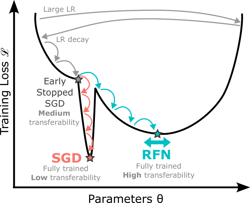
Figure 1 summarizes our contributions:

•

The learning rate decay allows the exploration of the loss landscape to go down the valley. After a few iterations, SGD reaches its best transferability (“early stopped SGD”, gray star). The sharpness is temporarily contained.
•

As training with SGD continues, sharpness increases and transferability decreases. The fully trained model (red star) is a suboptimal surrogate. SGD falls into deep, sharp holes where the representation is too specific.
•

RFN explicitly minimizes sharpness over a large neighborhood (thick blue arrow) and avoids undesirable holes. Transferability is maximum after a full training (blue star), and early stopping is not needed.

2 Related Work

Transferability techniques.

The transferability of adversarial examples is a prolific research topic [2, 4, 8, 9, 15, 16, 20, 24, 25, 28]. [28] recently categorizes of transferability techniques and recommend evaluating techniques by comparing them competitively within each category. Our evaluation follows this recommendation in Section 5. Gradient-based transferability techniques can be decomposed into model augmentation, data augmentation, attack optimizers, and feature-based attacks. In Section 5, we show that our method improves the following techniques when combined. Model augmentation adds randomness to the weights or the architecture to avoid adversarial examples too specific to a single representation: GN [15] uses dropout or skip erosion, SGM [24] favors gradients from skip connections during the backward pass, LGV [9] collects models along the SGD trajectory during a few additional epochs with a high learning rate. Data augmentation techniques transform the inputs during the attack: DI [25] randomly resizes the input, SI [16] rescales the input, VT [23] smooths the gradients locally. Attack optimizers smooth updates during gradient ascent with momentum (MI [4]) or Nesterov accelerated gradient (NI [16]).

Training surrogate models.

Despite the important amount of work on transferability, the way to train an effective single surrogate base model has received little attention in the literature [28]. [2, 18, 27] point that early stopping SGD improves transferability. [20] proposes SAT, slight adversarial training that uses tiny perturbations to filter out some non-robust features. [9] evaluates LGV-SWA, the weight average of the models collected by LGV. In Section 5, we evaluate these competitive techniques. Our approach sheds new light on the relation between flatness and transferability. [20] implicitly flattens the surrogate model, since adversarial trained models are flatter than their naturally trained counterparts [21]. We observe a similar implicit link with early stopping in Section 4. [9] proposes the surrogate-target misalignment hypothesis to explain why flat minima in the parameter space are better surrogate models. We improve on their single-model baseline (LGV-SWA) by explicitly minimizing sharpness, and we show that LGV, their full model augmentation technique, is complementary to ours.

Early stopping for transferability.

Several works [2, 27, 18] point out that fully trained surrogate models are not optimal for transferability. To explain this observation, they propose a hypothesis based on the perspective of robust and non-robust features (RFs/NRFs) from [10]. [10] disentangles features that are highly predictive and robust to adversarial perturbations (RFs), and features that are also highly predictive but non-robust to adversarial perturbations (NRFs). According to [2, 18], the training of DNNs mainly learns RFs first and then learns NRFs. NRFs are transferable [10], but also brittle. RFs in a tiny input neighborhood, called slightly RFs, improve transferability [27, 20]: the input neighborhood is sufficiently small for an attack to find adversarial examples in a larger radius, and slightly RFs are less brittle than NRFs. Models at earlier epochs would be composed of more slightly RFs, thus being better surrogate models. Section 3 provides some observations that tend to refute this hypothesis. Instead, Sections 4 and 5 suggest that the success of early stopping is correlated with the dynamics of the training and the flatness of the surrogate.

3 Another Look at the Non-Robust Features Hypothesis about Early Stopping

In this section, we point the flaws of the robust and non-robust features (RFs/NRFs) hypothesis [2, 27, 18] to explain the success of early stopping for transferability. According to this hypothesis, earlier representations are more transferable than their fully trained counterparts, because they contain more slightly RFs than NRFs. Slightly RFs are features that are robust to tiny worst-case perturbations, and NRFs are features that are not. See Section 2 for more details.

Early stopping indeed increases transferability.

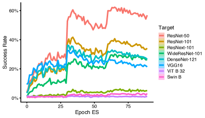
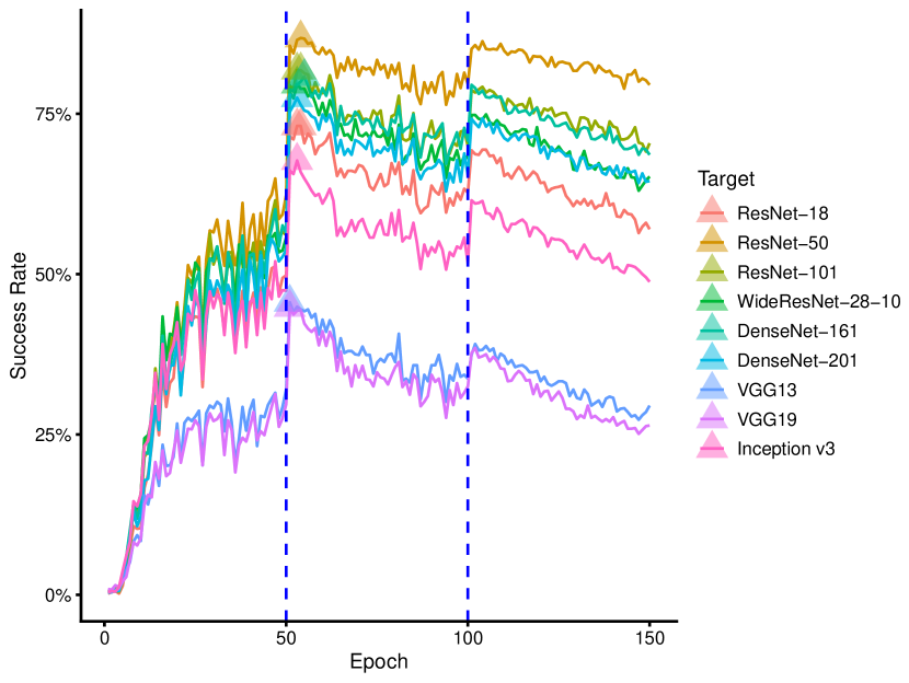
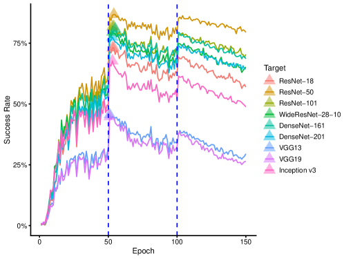
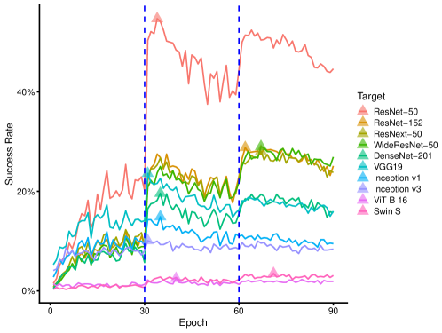
First, we check that a fully trained surrogate model is not optimal for transferability. We train two ResNet-50 surrogate models on the CIFAR-10 and ImageNet datasets using standard settings. Figure 2 reports the success rates on CIFAR-10 of the BIM attack applied at every epoch and evaluated on 19 fully trained target models (Section B in supp. materials for ImageNet). For both datasets and a variety of targeted architectures, the optimal epoch for transferability occurs around one or two thirds of training¹¹1Transferability decreases along epochs, except for the two vision transformers targets on ImageNet where the transferability is stable at the end of training.. Therefore, we confirm that early stopping increases transferability.

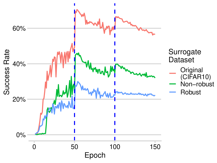
Early stopping improves transferability from both surrogates trained on robust and non-robust datasets.

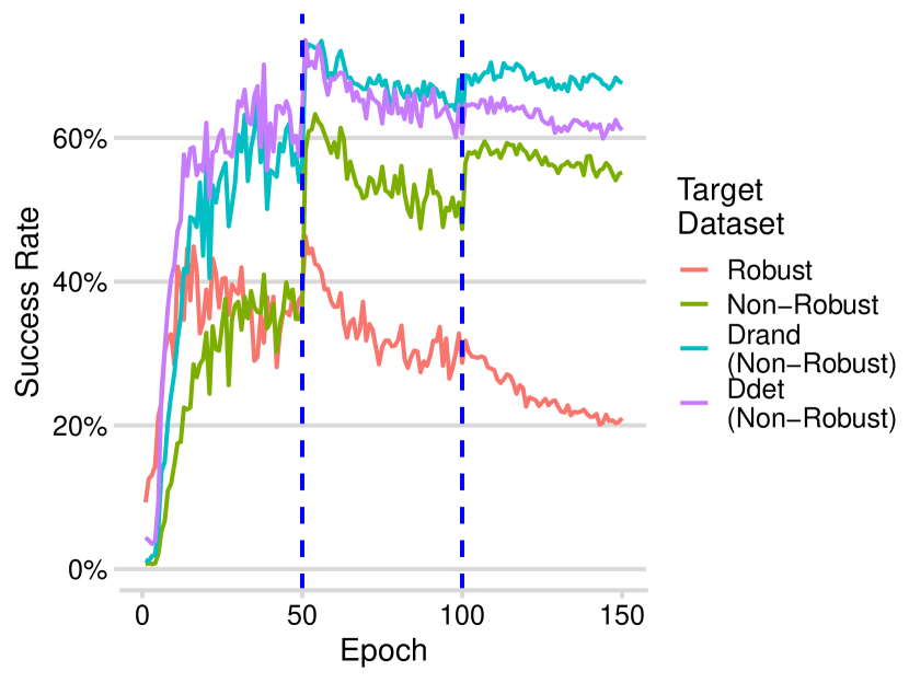
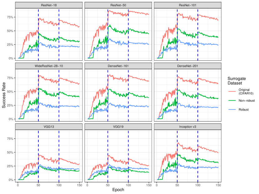
We show that early stopping works similarly well on surrogate models trained on robust and non-robust datasets. We retrieve the robust and non-robust datasets from [10], that are altered from CIFAR-10 to contain mostly RFs and, respectively, NRFs. We train two ResNet-50 models on both datasets with SGD and the same hyperparameters (reported in supp. materials). Figure 3 shows the transferability across training epochs. The success rates of both surrogate models evolve similarly (scaled by factor) to the model trained on the original dataset: transferability peaks around the epochs 50 and 100 and decreases during the following epochs. According to the RFs/NRFs hypothesis, we expected “X-shaped” transferability curves: increasing transferability from NRFs and strictly decreasing transferability from RFs (after initial convergence). The RFs/NRFs hypothesis does not describe why early learned NRFs are better for transferability than fully learned NRFs.

Early stopping improves transferability to both targets trained on robust and non-robust datasets.

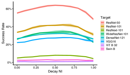
We observe that an early stopped surrogate model trained on the original dataset is best to target both targets composed of RFs and NRFs. Here, we keep the original CIFAR-10 dataset to train the surrogate model. We target four ResNet-50 models trained on the robust and non-robust datasets of [10]²²2In this experiment, we include two other non-robust datasets $D_{\text{rand}}$ and $D_{\text{det}}$ from [10]. By construction, the only useful features for classification are NRFs. We did not include them in the previous experiment because training on them is too unstable.. Figure 4 shows the same early stopped surrogate model is optimal for targeting both models composed of RFs and NRFs. Since the higher the transferability, the more similar the representations are, we conclude that the early trained representations are more similar to both RFs and NRFs than their fully trained counterparts.

Overall, we provide new evidence that early stopping for transferability acts similarly on robust and non-robust features. We do not observe an inherent trade-off between RFs and NRFs. Therefore, the hypothesis that early stopping favors RFs over NRFs does not hold. We conjecture that a phenomenon orthogonal to RFs/NRFs explains why fully trained surrogates are not optimal.

4 Transferability and Training Dynamics

This section explores the relationship between the training dynamics of the surrogate model and its transferability. In particular, we observe several phenomena following the learning rate step decays: transferability peaks, sharpness drops, and the exploration of the loss surface transitions phases.

Transferability peaks when the LR decays.

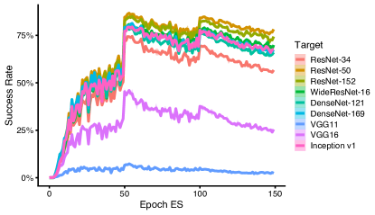
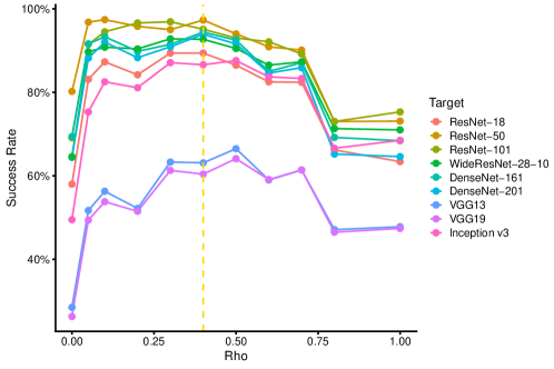
We point out the key role of the LR decay in the success of early stopping for transferability. The optimal number of surrogate training epochs for transferability occurs a couple of epochs after the decay of the LR. We train a ResNet-50 surrogate model for 150 epochs on CIFAR-10, using the standard LR schedule of [5] which divides the LR by 10 at epochs 50 and 100. For all nine targets considered individually, the highest transferability is between epochs 51 and 55 (Section B in supp. materials). Figure 5 shows that transferability suddenly peaks after the LR decay (red line). We train on ImageNet a ResNet-50 surrogate model for 90 epochs with LR decay at epochs 30 and 60. The highest transferability per target occurs either after the first decay (epochs 31 or 35) or after the second one (epochs 62 or 67), except for both vision transformer targets, where transferability plateaus at a low success rate after the second decay. Overall, the success of early stopping appears to be related to the exploration of the loss landscape, which is governed by the learning rate.

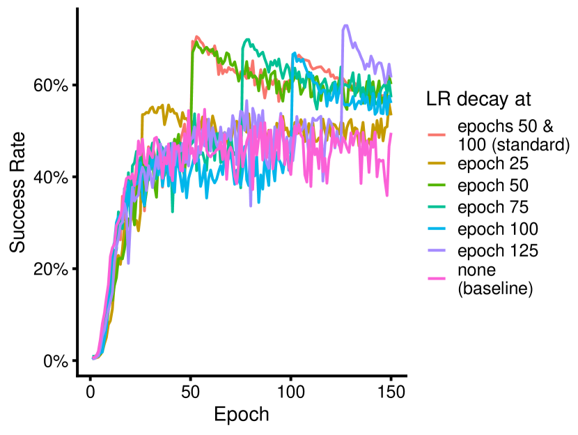
Consistency of the peak of transferability across training.

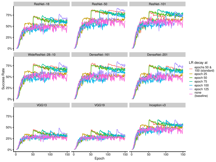
The peak of transferability described above can be consistently observed at any point of training (after initial convergence). Here, we modify the standard double decay LR schedule to perform a single decay at a specified epoch. The learning rate is constant (0.1) until the specified epoch, where it will be 10 times lower (0.01) for the rest of the training. We evaluate the transferability of five surrogates with a decay at, respectively, epoch 25, 50, 75, 100 and 125. In Figure 5, we observe a similar transferability peak for all these surrogates, except for the decay at epoch 25 where the decay occurs before the end of the initial convergence (details per target in Section D in supp. materials). We add as baseline the constant learning rate (at 0.1). Without LR decay, the transferability plateaus after initial convergence. Therefore, we conclude that the step decay of the LR enables early stopping to improve transferability.

Sharpness drops when the LR decays.

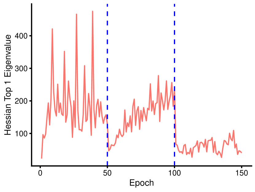
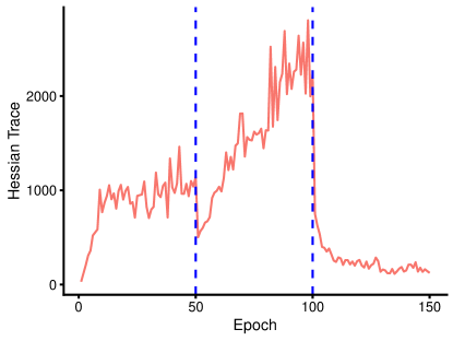
When the LR decays, the sharpness in the parameter space drops. We observe a drop of both worst-case sharpness and average sharpness, measures respectively by the largest eigenvalue and the trace of the Hessian. We compute both sharpness metrics at every epoch using the PyHessian library [26] on a random subset of a thousand examples from the CIFAR-10 train dataset. Figure 6 reproduces the largest Hessian eigenvalue. The Hessian trace is available in Section D in supp. materials. For both metrics, we observe that sharpness decreases abruptly and significantly immediately after both LR decays at epochs 50 and 100.

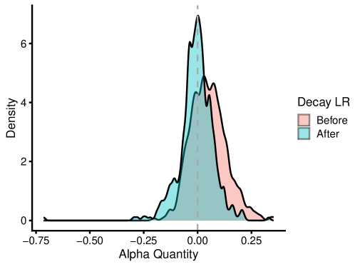
Crossing the valley before exploring the valley.

The LR decay corresponds to a transition from a “crossing the valley” phase to a “crawling down to the valley” phase described in [19]. [19] proposes the $\alpha$ -quantity, a metric computed at the level of SGD iterations to disentangle whether the iteration understeps or overshoots the minimum along the current step direction. Based on a noise-informed quadratic fit, $\alpha\approx 0$ indicates an appropriate LR that minimizes the loss in the direction of the gradient at this iteration (“going down to the valley”). $\alpha>0$ indicates that the current LR overshoots this minimum (“crossing the valley”). We compute the $\alpha$ -quantity every four SGD iterations during the best five epochs for transferability on CIFAR-10 (“after LR decay”, epochs 50–54) and during the five preceding epochs (“before LR decay”, epochs 45–49). The one-sided Welch Two Sample t-test has a p-value inferior to $2.2\mathrm{e}^{-16}$ . We reject the null hypothesis in favor of the alternative hypothesis that the true difference of $\alpha$ -quantity in means between the group “before LR decay” and the group “after LR decay” is strictly greater than 0³³3We also perform a one-sided Welch Two Sample t-test on the 5 epochs before and after the second LR decay (epochs 95–99 vs. epochs 100-105). Its p-value is equal to $0.004387$ . Using the Bonferroni correction, we compare the p-values of both individual tests with a significance threshold of 0.5%. We reject the null hypothesis for both LR decays with a significance level of 1%.. Section D in supp. materials contains the density plot of the $\alpha$ -quantities for both groups. Our results suggest that before the LR decay, training is slow due to a “crossing the valley” pattern. The best early stopped surrogate occurs a few training epochs after the LR decay when the SGD starts exploring the bottom of the valley.

We conclude that the effect of early stopping on transferability is tightly related to the dynamics of the exploration of the loss surface, governed by the learning rate. Overall, Figure 1 illustrates our observations:

1.

Before the LR decays, the training bounces back and forth crossing the valley from above (top gray arrows).
2.

After the LR decays, training goes down the valley. Soon after, SGD has its best transferability (“early stopped SGD” gray star). Sharpness is reduced.
3.

When learning continues, the training loss decreases and sharpness slowly increases. SGD finds a “deep hole” of the loss landscape, corresponding to a specific representation that has poor transferability (“fully trained SGD” red star).

5 Going Further: Flatness at the Rescue of SGD

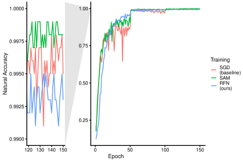
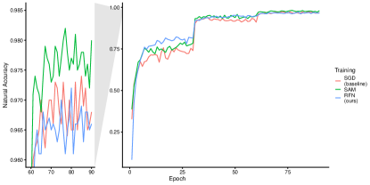
Since transferability peaks to its higher value when sharpness drops, we explore in this section how to improve transferability by explicitly minimizing the sharpness of the surrogate model. First, we show that SAM, sharpness-aware minimizer, finds surrogate models with high transferability at every epoch. Second, we propose a new transferability technique called RFN (Representation from Flat Neighbourhood), based on unusually large flat neighborhoods that avoid large holes on the surface of the loss landscape.

Sharpness-Aware Minimizer (SAM, [6]) minimizes the maximum loss around a neighborhood by performing a gradient ascent step followed by a gradient descent step. At the cost of one additional forward-backward pass per iteration, SAM avoids deep, sharp holes on the surface of the loss landscape [11]. We explore the use of SAM to train a surrogate model and show that:

1.

Explicitly minimizing sharpness improves transferability over SGD.
2.

The large flat neighborhoods used by RFN benefit specifically transferability (not natural generalization).
3.

Contrary to SGD, SAM and RFN benefit from a full-training. Thus, RFN does not need early stopping to train generic representations.

Minimizing sharpness improves transferability.

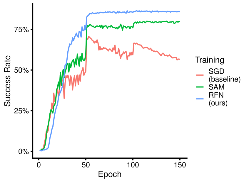
By explicitly minimizing sharpness in the parameter space, SAM trains better surrogate models than SGD. On CIFAR-10, we train a ResNet-50 model without any hyperparameter tuning, using the original SAM hyperparameter ( $\rho=0.05$ ). The success rate averages over the nine targets at 79.71%, compared to 56.66% for full training with SGD, and 70.54% for SGD at its best (epoch 53)⁴⁴4Note that this original SAM surrogate is trained without tuning hyperparameter for transferability. We show below that larger $\rho$ significantly improves it.. Similarly, on ImageNet, we train a ResNet-18 with SAM ( $\rho=0.05$ ) and obtain an average success rate on ten targets of 18.81%. A full training with SGD averages to 13.23%, and an early stopped one reaches 14.48% at its best (epoch 68). For both datasets, SAM consistently improves over fully trained and early stopped SGD for all our 19 targets (Section E in supp. materials).

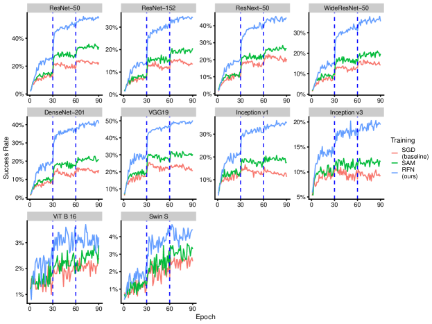
Large flat neighborhoods are optimal for transferability.

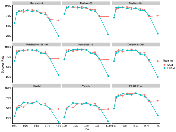
RFN significantly increases the transferability over the original SAM by minimizing sharpness over uncommonly large neighborhoods. The unique hyperparameter of SAM, $\rho$ , controls the size of the neighborhood where SAM minimizes sharpness. We evaluate the sensibility of transferability regarding this hyperparameter on CIFAR-10 (details in Section E in supp. materials). We find that SAM performs well for a broad range of $\rho$ values. The $\rho$ value selected on CIFAR-10 is also significantly beneficial on ImageNet. More importantly, using unusually large $\rho$ values significantly improves over the original SAM (Figure 7). The original SAM [6] uses a $\rho=0.05$ , [11] tunes it with a maximum of $0.2$ . On both CIFAR-10 and ImageNet, $\rho=0.4$ is best for transferability, i.e., a value twice larger than the maximum generally considered for natural generalization. Indeed, we observe that such large neighborhoods degrade natural accuracy. [11] shows that changing $\rho$ ends up in different basins. Therefore, RFN, i.e., SAM with high $\rho$ , finds neighborhoods that are specifically beneficial for transferability. It avoids large sharp holes on top of the loss surface.

RFN does not need early stopping.

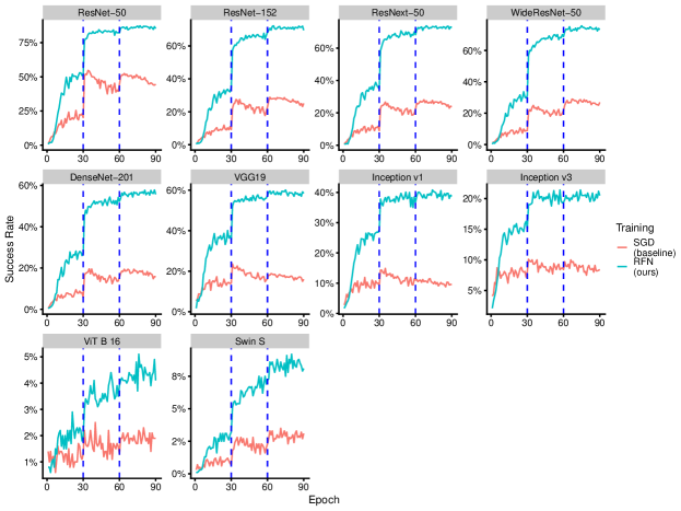
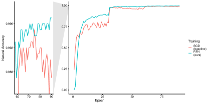
Training longer with RFN or SAM is both more stable than SGD and beneficial for transferability. In Figure 7, we report the success rate per training epoch for both SAM (green), RFN (blue), and SGD (red) on CIFAR-10. Contrary to SGD which needs to be carefully stopped to not train a suboptimal surrogate, the transferability of RFN and SAM increases or plateaus. These observations are also valid for ResNet-18 and ResNet-50 surrogates trained on ImageNet (Section E in supp. materials). RFN and SAM trainings are more stable, benefit from a full training, and do not require an error-prone stopping criterion.

On a side note, we also train three variants of SAM (ASAM, GSAM, AGSAM) [14, 29]. We did not get significant improvement over RFN (Section E in supp. materials).

Overall, RFN can avoid deep sharp minima in favor of unusually large flat neighborhoods containing more generic representations.

Table 1: Success rate on CIFAR-10 of competitive techniques to train a single surrogate model. Bold is best. Section F in supp. materials contains results with other perturbation norms. In %.

	Target
Surrogate	RN18	RN50	RN101	DN161	DN201	VGG13	VGG19	IncV3	WRN28
Fully Trained SGD	57.9	81.2	70.6	70.8	66.1	27.8	26.3	49.4	66.5
Early Stopped SGD	73.3	87.8	82.1	81.4	78.3	45.5	44.3	66.8	79.5
SAT [20]	66.3	76.2	73.6	66.9	66.1	49.8	48.5	57.9	67.8
RFN (ours)	89.7	97.3	95.5	95.7	94.0	63.6	60.6	87.3	93.0

Table 2: Success rate on ImageNet of competitive techniques to train a single surrogate model. Bold is best. Section F in supp. materials contains results with other perturbation norms. In %.

	Target
Surrogate	RN50	RN152	RNX50	WRN50	VGG19	DN201	IncV1	IncV3	ViT B	SwinS
Fully Trained SGD	44.5	25.2	24.8	27.1	16.2	16.4	9.8	8.0	1.8	3.3
Early Stopped SGD	51.5	27.4	27.7	28.0	18.4	18.7	10.8	10.4	2.2	2.7
LGV-SWA [9]	82.5	56.8	58.5	54.0	40.9	42.4	28.3	15.1	3.1	5.7
SAT [20]	76.3	62.5	66.8	63.4	48.1	59.0	47.9	40.8	17.4	16.8
RFN (ours)	85.7	70.3	73.3	73.2	58.2	55.6	37.9	20.5	4.0	8.2

Table 3: Success rate on ImageNet of three complementary categories of transferability techniques evaluated on ten targets. Underlined is worse when combined with RFN. Section F in supp. materials contains results with other perturbation norms. In %.

	Target
Attack	RN50	RN152	RNX50	WRN50	VGG19	DN201	IncV1	IncV3	ViT B	SwinS
Model Augmentation Techniques
GN [15]	68.0	43.1	41.3	44.1	24.8	27.2	14.3	9.9	1.9	3.8
GN+RFN	89.6	76.6	79.4	79.9	65.7	60.3	42.2	22.4	3.8	7.8
SGM [24]	62.8	40.6	41.5	43.5	31.9	28.0	19.3	13.2	4.1	7.9
SGM+RFN	83.2	68.7	71.5	73.0	67.0	56.2	48.9	26.6	6.2	13.6
LGV [9]	93.3	78.1	75.3	73.1	64.4	61.6	49.3	28.8	5.0	6.5
LGV+RFN	88.7	74.3	75.7	75.7	70.3	61.9	56.8	31.5	4.5	7.3
Data Augmentation Techniques
DI [25]	83.1	60.5	68.1	67.3	45.4	57.9	41.4	30.7	5.7	9.9
DI+RFN	95.0	89.7	90.7	91.6	85.3	87.8	87.5	64.2	14.2	19.0
SI [16]	60.0	37.9	37.3	40.0	23.9	30.0	19.6	13.5	2.6	3.8
SI+RFN	89.2	76.6	80.1	79.1	65.2	69.8	58.0	35.8	5.0	8.5
VT [23]	58.6	35.0	35.2	38.5	23.9	24.7	14.9	11.0	2.3	4.9
VT+RFN	92.0	81.2	82.4	82.9	72.3	72.3	56.7	33.6	7.0	13.5
Attack Optimizers
MI [4]	56.8	37.4	37.5	38.9	27.0	29.3	18.4	14.6	3.5	4.8
MI+RFN	89.4	79.3	80.4	80.8	71.5	71.1	60.1	39.3	8.5	15.2
NI [16]	53.7	33.1	32.9	35.1	20.5	20.8	12.2	9.4	1.8	3.9
NI+RFN	83.9	67.3	69.8	71.4	56.1	52.5	35.6	17.6	3.8	7.0

6 Evaluation of RFN

In this section, we show that RFN is an alternative to competitive techniques and complements other techniques well. To compare our technique to related work, we follow the good practices recommended by [28]: we evaluate each technique on its own with other comparable techniques that belong to the same category. First, we show that RFN is a competitive alternative to existing training techniques. Second, we show that RFN complements nicely transferability techniques. All our code and models are available on GitHub⁵⁵5https://github.com/Framartin/rfn-flatness-transferability.

RFN improves over competitive techniques.

We compare our RFN technique to competitive techniques that train a single representation. We aim to find training methods that can find generic representations that are good for transferability. We evaluate the model-augmentation transferability techniques in the next paragraph because avoiding the attack to overfit to a single model is an orthogonal objective. For a fair comparison, we choose the epoch of the early stopped SGD surrogate by evaluating a validation transferability at every training epoch. We craft one thousand adversarial examples from images of a validation set and evaluate them against a distinct set of target models. We retrieve the SAT (Slight Adversarial Training) ImageNet pretrained model used in [20], and we train it on CIFAR-10 using the same hyperparameters of adversarial training. LGV-SWA [9] is a single model defined by the weight average of the models collected by LGV. RFN uses $\rho=0.4$ for both datasets.

Tables 1 and 2 report the success rates of various techniques. On CIFAR-10, RFN strictly dominates the other methods for every target. RFN requires twice as many computations as SGD, but four times less than SAT⁶⁶6SAT [20] uses adversarial training with seven PGD steps on CIFAR-10. It needs a total of 8 backward-forward passes per training iteration. RFN always requires two.. On ImageNet, RFN beats the other techniques for 5 of the 10 targets. For the other targets, RFN is second after SAT. Still, RFN is an interesting alternative since SAT doubles the training computational budget compared to RFN. We leave as future work the combination of SAT and RFN by replacing SGD by SAM to update parameters during adversarial training.

RFN is a better base model for complementary techniques.

We show that RFN is a good base model to combine with existing model augmentation, data augmentation, and attack optimization transferability techniques. These categories target complementary objectives: model and data augmentations aim at reducing the tendency of the attack to overfit the base model by adding randomness to gradients. Attack optimizers intend to smooth the gradient updates. Table 3 presents the success rates of eight transferability techniques combined with our RFN base model on ImageNet. For every target, RFN provides a base model that improves every eight techniques, compared to the standard fully trained SGD surrogate. The only exception (underlined) is the combination with LGV for three of the ten targets. Since LGV collects models with SGD and a high learning rate, a conflict might occur when LGV continues training with SGD from a checkpoint trained with SAM. We leave for future work the evaluation of an LGV variant where models are collected with SAM and a high constant learning rate.

7 Conclusion

Overall, our insights into the behavior of SGD through the lens of transferability drive us to a new successful approach to train better surrogate models with limited computational overhead. Our observations lead us to reject the hypothesis that early stopping benefits transferability due to an inherent trade-off between robust and non-robust features. Instead, we explain the success of early stopping in relation to the dynamics of the exploration of the loss landscape. After the learning rate decays, SGD drives down the valley and progressively falls into deep, sharp holes. These fully trained representations are too specific to generate highly transferable adversarial examples. We remediate this issue by explicitly minimizing sharpness in an unusually large neighborhood. Avoiding those large sharp holes proves to be useful in improving transferability. Finally, we propose RFN, a competitive technique to train a surrogate model that nicely complements other existing transferability techniques.

References

[1] Arsenii Ashukha, Alexander Lyzhov, Dmitry Molchanov, and Dmitry Vetrov. Pitfalls of In-Domain Uncertainty Estimation and Ensembling in Deep Learning. 2 2020.
[2] Philipp Benz, Chaoning Zhang, and In So Kweon. Batch Normalization Increases Adversarial Vulnerability and Decreases Adversarial Transferability: A Non-Robust Feature Perspective. In ICCV 2021, 10 2021.
[3] Battista Biggio, Igino Corona, Davide Maiorca, Blaine Nelson, Nedim Šrndić, Pavel Laskov, Giorgio Giacinto, and Fabio Roli. Evasion attacks against machine learning at test time. In Lecture Notes in Computer Science (including subseries Lecture Notes in Artificial Intelligence and Lecture Notes in Bioinformatics), volume 8190 LNAI, pages 387–402, 8 2013.
[4] Yinpeng Dong, Fangzhou Liao, Tianyu Pang, Hang Su, Jun Zhu, Xiaolin Hu, and Jianguo Li. Boosting Adversarial Attacks with Momentum. In Proceedings of the IEEE Computer Society Conference on Computer Vision and Pattern Recognition, pages 9185–9193, 10 2018.
[5] Logan Engstrom, Andrew Ilyas, Shibani Santurkar, and Dimitris Tsipras. Robustness (Python Library), 2019.
[6] Pierre Foret, Ariel Kleiner Google Research, Hossein Mobahi Google Research, and Behnam Neyshabur Blueshift. Sharpness-Aware Minimization for Efficiently Improving Generalization. 10 2020.
[7] Ian J. Goodfellow, Jonathon Shlens, and Christian Szegedy. Explaining and Harnessing Adversarial Examples. 12 2014.
[8] Martin Gubri, Maxime Cordy, Mike Papadakis, Yves Le Traon, and Koushik Sen. Efficient and Transferable Adversarial Examples from Bayesian Neural Networks. In UAI 2022, 2022.
[9] Martin Gubri, Maxime Cordy, Mike Papadakis, Yves Le Traon, and Koushik Sen. LGV: Boosting Adversarial Example Transferability from Large Geometric Vicinity. In ECCV 2022, 2022.
[10] Andrew Ilyas, Shibani Santurkar, Dimitris Tsipras, Logan Engstrom, Brandon Tran, and Aleksander Madry. Adversarial Examples Are Not Bugs, They Are Features. 5 2019.
[11] Jean Kaddour, Linqing Liu, Ricardo Silva, and Matt J. Kusner. When Do Flat Minima Optimizers Work? In NeurIPS 2022, 2 2022.
[12] Hoki Kim. Torchattacks: A pytorch repository for adversarial attacks. arXiv preprint arXiv:2010.01950, 2020.
[13] Alexey Kurakin, Ian J. Goodfellow, and Samy Bengio. Adversarial examples in the physical world. In 5th International Conference on Learning Representations, ICLR 2017 - Workshop Track Proceedings, 7 2017.
[14] Jungmin Kwon, Jeongseop Kim, Hyunseo Park, and In Kwon Choi. ASAM: Adaptive Sharpness-Aware Minimization for Scale-Invariant Learning of Deep Neural Networks. 2 2021.
[15] Yingwei Li, Song Bai, Yuyin Zhou, Cihang Xie, Zhishuai Zhang, and Alan Yuille. Learning Transferable Adversarial Examples via Ghost Networks. Proceedings of the AAAI Conference on Artificial Intelligence, 34(07):11458–11465, 12 2018.
[16] Jiadong Lin, Chuanbiao Song, Kun He, Liwei Wang, and John E. Hopcroft. Nesterov Accelerated Gradient and Scale Invariance for Adversarial Attacks. 8 2019.
[17] Muzammal Naseer, Kanchana Ranasinghe, Salman Khan, Fahad Shahbaz Khan, and Fatih Porikli. On Improving Adversarial Transferability of Vision Transformers. In ICLR (spotlight), 3 2022.
[18] Vikram Nitin. SGD on Neural Networks learns Robust Features before Non-Robust, 3 2021.
[19] Frank Schneider, Felix Dangel, and Philipp Hennig. Cockpit: A Practical Debugging Tool for the Training of Deep Neural Networks. 2 2021.
[20] Jacob M. Springer, Melanie Mitchell, and Garrett T. Kenyon. A Little Robustness Goes a Long Way: Leveraging Robust Features for Targeted Transfer Attacks. Advances in Neural Information Processing Systems, 12:9759–9773, 6 2021.
[21] David Stutz, Matthias Hein, and Bernt Schiele. Relating Adversarially Robust Generalization to Flat Minima. Proceedings of the IEEE International Conference on Computer Vision, pages 7787–7797, 4 2021.
[22] Christian Szegedy, Wojciech Zaremba, Ilya Sutskever, Joan Bruna, Dumitru Erhan, Ian Goodfellow, and Rob Fergus. Intriguing properties of neural networks. 12 2013.
[23] Xiaosen Wang and Kun He. Enhancing the Transferability of Adversarial Attacks through Variance Tuning. Proceedings of the IEEE Computer Society Conference on Computer Vision and Pattern Recognition, pages 1924–1933, 3 2021.
[24] Dongxian Wu, Yisen Wang, Shu-Tao Xia, James Bailey, and Xingjun Ma. Skip Connections Matter: On the Transferability of Adversarial Examples Generated with ResNets. In ICLR, 2 2020.
[25] Cihang Xie, Zhishuai Zhang, Yuyin Zhou, Song Bai, Jianyu Wang, Zhou Ren, and Alan L. Yuille. Improving transferability of adversarial examples with input diversity. In Proceedings of the IEEE Computer Society Conference on Computer Vision and Pattern Recognition, volume 2019-June, pages 2725–2734, 3 2019.
[26] Zhewei Yao, Amir Gholami, Kurt Keutzer, and Michael W. Mahoney. PyHessian: Neural Networks Through the Lens of the Hessian. Proceedings - 2020 IEEE International Conference on Big Data, Big Data 2020, pages 581–590, 12 2019.
[27] Chaoning Zhang, Gyusang Cho, Philipp Benz, Kang Zhang, Chenshuang Zhang, Chan-Hyun Youn, and In So Kweon. Early Stop And Adversarial Training Yield Better surrogate Model: Very Non-Robust Features Harm Adversarial Transferability, 2021.
[28] Zhengyu Zhao, Hanwei Zhang, Renjue Li, Ronan Sicre, Laurent Amsaleg, and Michael Backes. Towards Good Practices in Evaluating Transfer Adversarial Attacks. 11 2022.
[29] Juntang Zhuang, Boqing Gong, Liangzhe Yuan, Yin Cui, Hartwig Adam, Nicha C Dvornek, sekhar tatikonda, James s Duncan, and Ting Liu. Surrogate Gap Minimization Improves Sharpness-Aware Training. In International Conference on Learning Representations, 2022.

Supplementary Materials

These supplementary materials contain the following sections:

•

Appendix A details the experimental settings,
•

Appendix B reports the transferability and the natural accuracy by epochs of surrogate trained with SGD on CIFAR-10 and ImageNet,
•

Appendix C reports additional results of Section 3 “Another Look at the Non-Robust Features Hypothesis about Early Stopping”,
•

Appendix D reports additional results of Section 4 “Transferability and Training Dynamics”,
•

Appendix E reports additional results about the role of the size of flat neighborhoods, three SAM variants, and about SAM on ImageNet,
•

Appendix F reports additional results of Section 6 “Evaluation of RFN” with other adversarial perturbation norms,
•

Appendix G reports the results regarding the selection of the hyperparameters of transferability techniques.

Appendix A Experimental Settings

This section describes the experimental settings used in this article. The experimental setup is standard for transfer-based attacks.

•

Our source code used to train and evaluate models is publicly available on GitHub at this URL: https://github.com/Framartin/rfn-flatness-transferability.
•

Our trained models on both CIFAR-10 and ImageNet are publicly distributed through HuggingFace at this URL: https://huggingface.co/mgubri/rfn-flatness-transferability.

Target models.

All our target models on CIFAR-10 are fully trained for 150 epochs with SGD using the hyperparameters reported in Table 4. For a fair comparison, the baseline surrogate is trained with SGD using the same hyperparameters as the targets. On ImageNet, the target models are the pretrained models distributed by PyTorch. On CIFAR-10, we target the following nine architectures: ResNet-50 (the surrogate with the same architecture is an independently trained model), ResNet-18, ResNet-101, DenseNet-161, DenseNet-201, WideResNet-28-10, VGG13, VGG19, and Inception v3. The ten target architectures on ImageNet are the following: ResNet-50, ResNet-152, ResNeXt-50 32X4D, WideResNet-50-2, DenseNet-201, VGG19, GoogLeNet (Inception v1), Inception v3, ViT B 16 and Swin S. Additionally, we train a “validation” set of architectures on CIFAR-10 to select hyperparameters independently of reported results. This set is composed of: ResNet-50 (another independently trained model), ResNet-34, ResNet-152, DenseNet-121, DenseNet-169, WideResNet-16-8, VGG11, VGG16, and GoogLeNet (Inception v1). This validation set of target models on ImageNet is composed of the following architectures: ResNet-50 (another independently trained model), ResNet-101, ResNeXt-101 64X4D, WideResNet101-2, VGG16, DenseNet121, ViT B 32 and Swin B.

Surrogate models trained with SGD.

We train the surrogate models on CIFAR-10 and ImageNet using SGD with the standard hyperparameters of the robustness library [5] (Table 4). Due to computational limitations on ImageNet, we limit the number of epochs to 90, reusing the same hyperparameters as [1].

Surrogate models trained with SAM/RFN.

We train surrogate models with SAM using the same hyperparameters as the models trained with SGD for both datasets. We integrate the SAM optimizer into the robustness library [5]. The unique hyperparameter of SAM is $\rho$ which is set to $0.05$ as the original paper for both datasets for the original SAM surrogate. The RFN surrogate is trained with SAM and $\rho$ equal to $0.4$ .

Surrogate models of competitive techniques (Section 6).

To compare with competitive training techniques on ImageNet, we retrieve the original models of LGV-SWA [9], weights averaged over 10 additional epochs with a high learning rate of $0.1$ , and SAT [20], an adversarially trained model with a small maximum $L_{2}$ norm perturbation $\varepsilon$ of $0.1$ and with the PGD attack applied with 3 steps and a step size equals to $2\varepsilon/3$ . On CIFAR-10, we reuse the best hyperparameters of [20] to adversarially train the SAT surrogate model with a maximum $L_{2}$ norm $\varepsilon$ of $0.025$ and PGD with 7 steps and a step size of $0.3\varepsilon$ . For a fair comparison, we choose the best checkpoint of the early stopped SGD surrogate by evaluating the transferability of every training epoch. For each epoch, we craft 1,000 adversarial examples from a distinct validation set of original examples and compute their success rate over a distinct set of validation target architectures. On CIFAR-10, the selected epoch is 54, and 66 on ImageNet. All the other hyperparameters not mentioned in this paragraph are the same as those used to train the surrogates with SGD.

Transferability Techniques.

For a fair comparison with existing transferability techniques, we select their hyperparameter by cross-validation: we compute the success rate on a validation set of targets from a distinct set of natural examples. Section G contains the details and the hyperparameters selected for the eight transferability techniques considered, i.e., early stopping, GN, SGM, LGV, DI, SI, VT, MI, and NI.

Attack.

Unless specified otherwise, we use the BIM (Basic Iterative Method) [13] which is the standard attack for transferability [2, 4, 8, 9, 15, 16, 20, 24, 25, 28]. By default, the maximum $L_{\infty}$ perturbation norm $\varepsilon$ is set to $4/255$ . We use the BIM hyperparameters tuned by [8, 9] on a distinct set of validation target models: BIM performs 50 iterations with a step size equal to $\varepsilon/10$ . Unless specified otherwise, we craft adversarial examples from a subset of 1,000 natural test examples that are correctly predicted by all the target models. The success rate is the misclassification rate of these adversarial examples evaluated on one target model.

Threat model.

We study the threat model of untargeted adversarial examples: the goal of the adversary is misclassification. We consider the standard adversary capability for transfer-based black-box attacks, where the adversary does not have query access to the target model. Query-based attacks are another distinct family of attacks.

Implementation.

The source code of every experiment is available on GitHub. Our models are distributed through HuggingFace. We use the torchattacks library [12] to craft adversarial examples with the BIM attacks and four transferability techniques, namely LGV, DI, SI, VT, MI and NI. We reuse the original implementations of GN and SGM to “patch” the surrogate architecture, and use the TorchAttacks implementation of BIM on top. The software versions are the following: Python 3.10.8, PyTorch 1.12.1, Torchvision 0.13.1, and TorchAttacks 3.3.0.

Infrastructure.

For all experiments, we use Tesla V100-DGXS-32GB GPUs on a server with 256GB of RAM, CUDA 11.4, and the Ubuntu operating system.

Table 4: Hyperparameters used to train surrogate models.

Training	Hyperparameter	Dataset	Value
All	Number of epochs	CIFAR-10	150
	Number of epochs	ImageNet	90
	Initial learning rate	All	0.1
	Learning rate decay	CIFAR-10	Step-wise /10 each 50 epochs
	Learning rate decay	ImageNet	Step-wise /10 each 30 epochs
	Momentum	All	0.9
	Batch-size	CIFAR-10	256
	Batch-size	ImageNet	128
	Weight decay	CIFAR-10	0.0005
	Weight decay	ImageNet	0.0001
SAM	$\rho$	All	0.05 for SAM, 0.4 for RFN

Appendix B Transferability and Natural Accuracy by Epochs

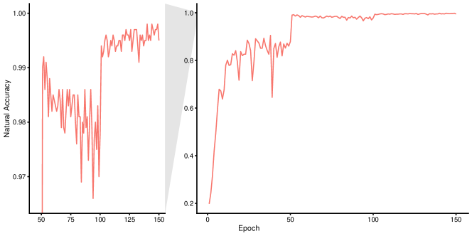
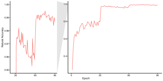
Early stopping clearly benefits transferability for all nine targets on CIFAR-10 and all ten targets on ImageNet (except for the two Vision Transformers, where the transferability plateaus). We reproduce below the success rates for all target models from the ResNet-50 surrogate model on both CIFAR-10 (Figure 8) and ImageNet (Figure 10) datasets. We also report the evolution of the natural accuracy for both CIFAR-10 (Figure 9) and ImageNet (Figure 11).

Appendix C Another Look at the Non-Robust Features Hypothesis about Early Stopping

This section contains detailed results of Section 3. Figure 12 reports the transferability per target of the experiment that shows the success of early stopping for surrogates trained on both robust and non-robust datasets.

Appendix D Transferability and Training Dynamics

This section contains additional results of Section 4 on the relationship between the training dynamics of the surrogate model and its transferability. Figure 13 contains the transferability per target of the surrogate models trained with a single learning rate decay at a varying epoch. The consistency of the peak of transferability across training epochs is valid for all nine targets. Figure 14 reproduces the trace of the Hessian for all training epochs of our standard surrogate model trained with SGD on CIFAR-10. This metric represents the average-case sharpness in parameter space. Sharpness drops when the learning rate decays, similarly to the worst-case sharpness reported in Section 4. Finally, Figure 15 is the density plot of the $\alpha$ -quantity before and after the decay of the learning rate, as described in Section 4.

Appendix E Choice of SAM Hyperparameters and its Variants

In this section, we show that:

1.

training the surrogate model with SAM improves transferability for a broad range of $\rho$ values, its unique hyperparameter that governs the size of flat neighbourhoods,
2.

large flat neighborhoods found by RFN improves transferability over the original SAM and degrades natural accuracy,
3.

among three SAM variants considered, none strictly dominates RFN,
4.

the transferability of RFN, SAM and SGD evolves along epochs similarly on ImageNet than on CIFAR-10.

E.1 The size of flat neighbourhoods: the choice of the $\rho$ hyperparameter

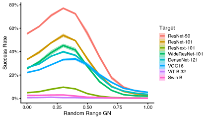
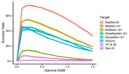
SAM has similar transferability for a wide range of its unique $\rho$ hyperparameter. Table 5 shows that the success rates on our test targets vary less than a percentage point for $\rho$ between $0.3$ and $0.5$ . Figure 16 shows that the improvements from SAM holds for all targets in this same range. Moreover, SAM with any $\rho$ value clearly dominates the SGD baseline. SAM is robust to a badly selected hyperparameter. Therefore, the risk of worsening transferability by switching from SGD to SAM to train the surrogate model is very limited.

For RFN, we select $\rho=0.4$ based on a separate set of architectures for the target models and a disjoint subset of original examples (Table 5, see Section A for more details about the experimental setting). We use the same $\rho=0.4$ for RFN on ImageNet without an additional hyperparameter selection.

Table 5 and Figure 16 show that the unusually large flat neighborhood ( $\rho=0.4$ ) used by RFN benefits all targets compared to the original SAM ( $\rho=0.05$ ). The latter is best for natural accuracy (Figure 16), suggesting that such large flat neighborhoods are specifically related to transferability.

Table 5: SAM improves transferability for a wide range of its unique

\rho

hyperparameter. Average success rate on nine targets of surrogates trained using SAM with various values of its

\rho

hyperparameter on CIFAR-10. The “Validation” and “Test” columns use distinct sets of targeted architectures and distinct subsets of original examples. All surrogate models are trained for 150 epochs on CIFAR-10.

\rho=0

corresponds to the baseline of the fully trained standard SGD surrogate. In %.

Value of $\rho$	Validation Success Rate	Test Success Rate
0.00 (SGD baseline)	55.59	56.61
0.05 (original SAM)	78.06	79.70
0.10	80.08	83.10
0.20	78.62	81.11
0.30	81.65	85.36
0.40 (RFN, best for transferability)	81.68	85.88
0.50	81.64	85.14
0.60	77.36	80.38
0.70	76.56	80.90
0.80	59.47	64.23
1.00	58.63	64.39

E.2 SAM and its variants

We train three variants of SAM (ASAM, GSAM, AGSAM) proposed by [14, 29], but we did not find a significant improvement over RFN. We try GSAM for various values of the $\rho$ hyperparameter. Figure 18 shows that GSAM does not significantly improve transferability over SAM. GSAM is more sensitive to very large neighborhoods ( $\rho=1.0$ ) where the SGD surrogate baseline is significantly better for all targets. Therefore, we do not consider GSAM for RFN.

Additionally, we train two additional variants ASAM, an adaptive variant of SAM, and AGSAM, an adaptive variant of GSAM. We follow the original paper [14] to select the $\rho$ hyperparameter: the authors recommend multiplying $\rho$ by 10 when switching to an adaptive variant. We use $\rho=4$ for ASAM and AGSAM. Table 6 shows that ASAM has a slightly higher average success rate than RFN (0.29 percentage point). But ASAM improves over RFN only for four of our nine target models. The AGSAM surrogate is better than RFN only for two of our nine targets and decreases the average success rate by more than one percentage point compared to RFN. We did base RFN on top of ASAM, but ASAM might be a promising direction for future work.

Table 6: None of the three SAM variants strictly dominates RFN. Average success rate on the nine targets of a ResNet-50 surrogate model trained using SAM variants on CIFAR-10. The “better than RFN” column reports the number of targets where the SAM variant in the corresponding row has higher transferability than RFN. Adversarial examples are crafted from a subset of 1,000 original examples from the test set. We train all surrogates for 150 epochs.

Training	Success Rate (%)	Better than RFN
SGD (baseline)	56.66	0 / 9
SAM (original)	79.71	0 / 9
RFN (ours)	85.88	—
GSAM (rho=0.4)	83.52	0 / 9
ASAM (rho=4)	86.17	4 / 9
AGSAM (rho=4)	84.57	2 / 9

E.3 SAM/RFN on ImageNet

The conclusions about RFN, SAM and SGD made on CIFAR-10 hold on ImageNet: RFN and SAM have higher transferability than both fully trained and early stopped SGD, RFN and SAM do not need early stopping, and RFN is better for transferability than the original SAM. Figures 19 and 21 report the success rates along epochs on ImageNet, respectively, from a ResNet-50 and ResNet-18 surrogate. Due to computational limitations, we only train the original SAM with the ResNet-18 architecture. We apply RFN on ImageNet without any hyperparameter selection. Despite this disadvantage, the observations on CIFAR-10 holds with the same size of neighborhood on ImageNet for both architectures.

Appendix F Evaluation of RFN

This section extends the evaluation of RFN of Section 6, performed with $\varepsilon$ equal to $4/255$ , to two other perturbation $L_{\infty}$ norms: $2/255$ and $8/255$ .

Evaluation against competitive techniques.

Tables 7 and 8 evaluate competitive techniques of RFN on CIFAR-10 with, respectively, maximum perturbations $L_{\infty}$ norm $\varepsilon$ of $2/255$ and $8/255$ . The same conclusions made with perturbations of size $4/255$ hold for these two norms: RFN clearly improves transferability. RFN beats other competitive techniques for all nine targets and both norms. The same conclusions on ImageNet made in Section 6 hold for these two norms. Tables 9 and 10 show respectively that RFN beats the other techniques in 6 out of 10 targets for $\varepsilon$ equal to $2/255$ , and in 5 out of 10 targets for $\varepsilon$ equal to $8/255$ .

Evaluation with complementary techniques.

Tables 11 and 12 extend the evaluation of complementary transferability techniques on ImageNet to, respectively, $2/255$ and $8/255$ norms. The conclusions of Section 6 hold in both cases. RFN increases the transferability of every eight techniques against every ten targets when combined, except for LGV on 4 targets using $\varepsilon$ equals $2/255$ , and LGV on 3 targets with $\varepsilon$ equals $2/255$ . Again, since LGV collects models with SGD and a high learning rate, a conflict might occur when LGV continues training with SGD from a checkpoint trained with SAM. Future work may explore the adaptation of the LGV model collection to SAM.

Table 7: Success rate on CIFAR-10 of competitive techniques to train a single surrogate model. Adversarial examples evaluated on nine targets with a maximum perturbation

L_{\infty}

norm

\varepsilon

2/255

. Bold is best. In %.

	Target
Surrogate	RN18	RN50	RN101	DN161	DN201	VGG13	VGG19	IncV3	WRN28
Fully Trained SGD	24.2	44.7	35.6	33.3	31.4	9.6	9.2	22.6	30.8
Early Stopped SGD	28.6	46.1	38.6	36.3	34.6	12.7	13.0	27.1	34.9
SAT	19.7	27.3	25.4	20.1	20.3	13.4	13.5	17.6	20.5
RFN (ours)	45.4	67.1	60.6	58.9	55.8	20.5	19.8	45.0	54.1

Table 8: Success rate on CIFAR-10 of competitive techniques to train a single surrogate model. Adversarial examples evaluated on nine targets with a maximum perturbation

L_{\infty}

norm

\varepsilon

8/255

. Bold is best. In %.

	Target
Surrogate	RN18	RN50	RN101	DN161	DN201	VGG13	VGG19	IncV3	WRN28
Fully Trained SGD	88.3	97.4	92.4	93.9	91.4	64.2	60.5	79.3	91.9
Early Stopped SGD	97.8	99.6	98.8	98.9	98.4	89.1	87.5	95.6	98.8
SAT	97.0	98.7	98.0	97.1	96.4	90.2	89.2	93.2	97.1
RFN (ours)	99.7	100.0	100.0	100.0	99.9	96.6	95.6	99.6	99.9

Table 9: Success rate on ImageNet of competitive techniques to train a single surrogate model. Adversarial examples evaluated on ten targets with a maximum perturbation

L_{\infty}

norm

\varepsilon

2/255

. Bold is best. In %.

	Target
Surrogate	RN50	RN152	RNX50	WRN50	VGG19	DN201	IncV1	IncV3	ViT B	SwinS
Fully Trained SGD	18.7	9.4	10.0	9.3	7.6	5.8	4.8	5.2	1.1	1.4
Early Stopped SGD	23.8	10.7	10.6	10.6	8.7	6.8	5.6	6.1	1.1	1.5
LGV-SWA	49.3	24.8	25.0	21.7	18.5	16.8	11.6	7.9	1.4	1.5
SAT	30.0	19.2	24.4	20.6	18.4	20.2	20.0	16.6	4.9	4.4
RFN (ours)	53.3	34.3	37.5	38.3	30.7	25.0	16.6	10.8	1.7	3.8

Table 10: Success rate on ImageNet of competitive techniques to train a single surrogate model. Adversarial examples evaluated on ten targets with a maximum perturbation

L_{\infty}

norm

\varepsilon

8/255

. Bold is best. In %.

	Target
Surrogate	RN50	RN152	RNX50	WRN50	VGG19	DN201	IncV1	IncV3	ViT B	SwinS
Fully Trained SGD	77.5	52.9	51.1	55.0	33.4	36.9	21.1	15.2	3.7	6.7
Early Stopped SGD	82.0	56.8	54.6	59.2	35.9	41.1	24.8	18.3	3.6	5.9
LGV-SWA	96.9	87.7	87.1	84.9	65.4	72.8	56.8	31.2	7.0	12.3
SAT	95.4	92.6	93.0	92.8	79.0	90.1	79.1	66.3	38.5	39.1
RFN (ours)	97.6	92.8	93.8	95.3	83.2	85.5	71.2	42.3	9.1	19.0

Table 11: Success rate on ImageNet of three complementary categories of transferability techniques evaluated on ten targets with a maximum perturbation

L_{\infty}

norm

\varepsilon

2/255

. Underlined is worse when combined with RFN. In %.

	Target
Attack	RN50	RN152	RNX50	WRN50	VGG19	DN201	IncV1	IncV3	ViT B	SwinS
Model Augmentation Techniques
GN	34.6	17.9	17.4	18.0	12.7	10.4	8.1	6.3	1.3	2.0
GN+RFN	59.7	42.2	42.8	45.4	35.4	29.1	18.3	11.0	1.8	2.4
SGM	26.9	14.9	15.2	15.8	15.5	9.7	7.4	6.6	1.6	3.6
SGM+RFN	46.3	32.0	33.8	35.5	33.4	21.8	20.3	11.9	2.7	5.6
LGV	59.8	33.0	32.9	28.4	31.1	24.2	21.3	12.5	2.4	2.6
RFN+LGV	50.7	31.3	32.9	31.4	33.5	27.9	25.0	14.3	2.1	2.5
Data Augmentation Techniques
DI	46.1	27.2	30.9	30.3	22.4	24.8	17.8	15.0	2.5	4.1
DI+RFN	66.6	49.5	57.1	52.3	54.1	49.3	47.5	31.8	4.4	6.9
SI	26.2	14.2	14.3	13.3	10.4	11.3	8.4	7.3	0.9	1.4
SI+RFN	56.5	37.9	42.9	41.2	33.0	31.4	25.0	14.7	2.1	2.9
VT	26.5	14.4	14.1	13.6	10.8	10.1	6.1	6.3	1.3	2.2
VT+RFN	61.5	43.0	47.0	47.4	39.4	35.9	24.3	13.3	2.1	4.9
Attack Optimizers
MI	29.8	15.9	16.4	16.2	12.6	11.5	7.7	8.0	1.9	2.7
MI+RFN	58.2	41.5	45.4	44.6	39.8	35.8	28.9	17.4	2.8	5.4
NI	21.1	11.0	10.9	11.2	8.4	6.9	5.0	5.2	1.3	1.7
NI+RFN	44.1	28.5	30.7	32.0	25.9	19.6	11.9	9.1	1.3	2.4

Table 12: Success rate on ImageNet of three complementary categories of transferability techniques evaluated on ten targets with a maximum perturbation

L_{\infty}

norm

\varepsilon

8/255

. Underlined is worse when combined with RFN. In %.

	Target
Attack	RN50	RN152	RNX50	WRN50	VGG19	DN201	IncV1	IncV3	ViT B	SwinS
Model Augmentation Techniques
GN	92.0	73.3	69.7	74.5	45.8	50.4	29.8	19.2	3.2	7.1
GN+RFN	98.2	96.5	96.5	97.4	87.3	88.3	74.4	42.9	9.0	19.4
SGM	91.2	78.4	76.2	79.2	65.1	59.7	48.2	29.1	8.9	19.6
SGM+RFN	97.3	95.1	96.4	96.5	91.5	88.7	84.8	59.8	18.9	32.8
LGV	99.6	97.4	95.9	95.7	87.7	91.7	79.9	47.9	8.9	16.4
LGV+RFN	99.0	96.5	96.2	96.7	90.7	91.0	85.7	53.8	9.5	17.7
Data Augmentation Techniques
DI	96.1	90.7	91.8	91.4	74.1	88.1	72.4	55.0	14.2	20.4
DI+RFN	99.8	99.6	99.5	99.7	98.6	99.3	98.4	90.4	34.7	48.7
SI	90.4	70.0	69.9	71.9	47.8	60.2	42.6	29.3	6.5	10.3
SI+RFN	98.9	97.3	97.3	98.0	89.9	94.8	90.1	67.2	15.0	23.6
VT	79.6	62.8	61.1	63.5	41.9	48.4	32.2	23.3	6.3	10.5
VT+RFN	98.0	96.7	96.1	97.3	92.9	93.1	87.1	64.2	20.0	39.2
Attack Optimizers
MI	83.3	60.9	63.3	64.3	48.7	53.8	39.2	30.4	7.4	11.7
MI+RFN	98.5	96.3	96.7	97.1	91.9	92.7	88.1	68.6	21.3	31.5
NI	86.2	65.3	65.1	70.3	43.6	47.1	28.7	19.6	4.7	8.3
NI+RFN	97.9	94.0	95.0	96.0	87.3	86.2	74.2	42.6	10.7	21.0

Appendix G Tuning Hyperparameters of Transferability Techniques

In this section, we tune the hyperparameters of the transferability techniques. For a fair comparison, we optimize the hyperparameters only on our fully trained SGD surrogate baseline. We do not optimize them for our RFN surrogate model. We craft adversarial examples from a distinct subset of 1,000 natural examples and evaluate them against six targeted architectures on ImageNet. We select the hyperparameter with the highest average success rate among the validation targets and three random seeds, except for Early Stopping, VT and DI where a single random seed is used due to computational limitations. Table 13 summarizes the hyperparameter selected.

Table 13: Hyperparameters of transferability techniques used.

Dataset	Technique	Hyperparameter	Value
Early Stopping	ImageNet	Epoch	66
Early Stopping	CIFAR-10	Epoch	54
GN	ImageNet	Random range	$[1-0.3,1+0.3]$
SGM	ImageNet	$\gamma$	0.2
LGV	ImageNet	Epochs	5
LGV	ImageNet	Learning rate	0.05
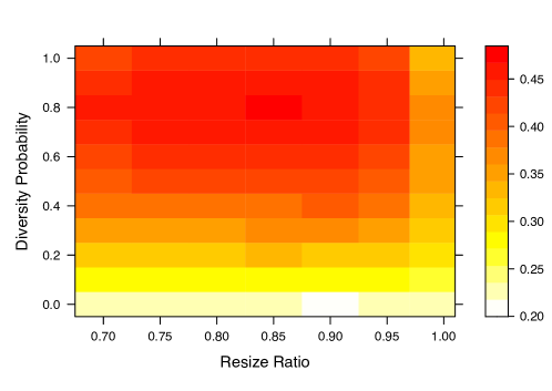
DI	ImageNet	Minimum resize ratio	85%
DI	ImageNet	Probability transformation	80%
SI	ImageNet	Number of copies $m$	4
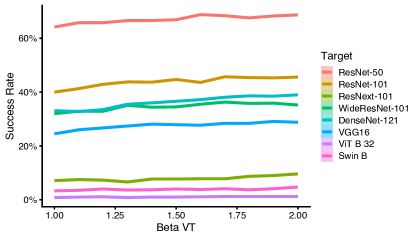
VT	ImageNet	$\beta$	1.8
VT	ImageNet	Number of copies $N$	20
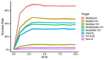
MI	ImageNet	Decay	1.2
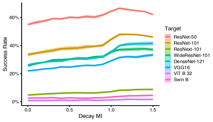
NI	ImageNet	Decay	0.6