The research was supported by the Academy of Finland. K. Myyryläinen and J. Weigt have also been supported by the Magnus Ehrnrooth Foundation.
C. Pérez is supported by grant PID2020-113156GB-I00, Spanish Government; by the Basque Government through grant IT1615-22
and the BERC 2014-2017 program and by the BCAM Severo Ochoa accreditation CEX2021-001142-S, Spanish Government.
J. Weigt is also supported by the European Union’s Horizon 2020 research and innovation programme (Grant agreement No. 948021).
We are very grateful to the Department of Mathematics at Aalto University for its support where the initiation of this research took place. In particular, we are very grateful to Juha Kinnunen for his support and for the discussions we had.
1. Introduction
The classical -Poincaré–Sobolev inequality states that
| (1) |
|
|
|
where , , , is a cube and is a dimensional constant.
In 2002, Bourgain, Brezis and Mironescu [3] proved the following fractional -Poincaré inequality
| (2) |
|
|
|
where , , , , is a cube and is a dimensional constant.
Note the factor in front of the fractional term which balances the limiting behaviour of the right-hand side when .
In particular, it was shown by Brezis [4] that without the factor the right-hand side of 2 is infinite for non-constant functions when .
Moreover, Bourgain, Brezis and Mironescu [2] showed that with this factor the fractional term coincides with the norm of the gradient when .
This means that in the limit 2 turns into the classical Poincaré inequality 1.
Later,
Maz’ya and Shaposhnikova [19]
proved the corresponding inequality in .
They showed in that the fractional term multiplied with coincides with the norm of the function when .
For other limiting behaviour results,
we refer to
Alberico, Cianchi, Pick and Slavíková [1],
Brezis, Van Schaftingen and Yung [5],
Drelichman and Durán [9]
and
Karadzhov, Milman and Xiao [17].
The existing proofs of the fractional Poincaré inequality apply Fourier analysis techniques [3], Hardy type inequalities [19] or
compactness arguments [23].
We give a new direct and transparent proof
using
a relative isoperimetric inequality as our main tool.
We concentrate on the case in 2.
Our approach is based on a new fractional type isoperimetric inequality in Lemma 3.3 which
can be seen as an improvement of the classical relative isoperimetric inequality, see Remark 3.4.
To our knowledge this approach with isoperimetric inequalities has not been considered in the fractional case before.
This allows further investigation of the theory of fractional Poincaré inequalities.
It is known that the classical -Poincaré inequality implies the classical -Poincaré inequality.
We investigate this in the fractional setting with weights.
The strategy is to first show that the fractional -Poincaré inequality implies the fractional -Poincaré inequality in Corollary 5.2.
Then we apply a self-improving property and a fractional truncation method to obtain the fractional -Poincaré inequality with weights, see Theorem 5.7 and Theorem 5.9.
This extends the fractional Poincaré inequality
in Hurri-Syrjänen, Martínez-Perales, Pérez and Vähäkangas [15]
from weights to weights.
Self-improving results are discussed in
Canto and Pérez [6],
Franchi, Pérez and Wheeden [13],
Lerner, Lorist and Ombrosi [18]
and Pérez and Rela [22].
For fractional truncation methods, see
Chua [8],
Dyda, Ihnatsyeva and Vähäkangas [10],
Dyda, Lehrbäck and Vähäkangas [11]
and Maz’ya [20].
Our proof for the fractional Poincaré inequality also works when we measure the oscillation against a Radon measure .
Our main result Theorem 4.1 states that
|
|
|
for , and where is the fractional maximal function with .
This extends [15, Theorem 2.10] to all values and exponents .
Weighted classical Poincaré inequalities have been studied extensively
starting from the classical result by Meyers and Ziemer [21]
and generalized to
| (3) |
|
|
|
for ,
by Franchi, Pérez and Wheeden in [14].
With Theorem 4.1 we extend their results to the fractional setting and are also able to deduce their original results from ours, see Corollaries 4.3 and 6.5.
Moreover, in [14] they show 3 in two separate ranges of and their constant blows up when .
In our argument, is uniformly bounded in and depends only on the dimension.
We also give an alternative proof by applying the relative isoperimetric inequality to highlight the differences between the classical and the fractional Poincaré inequalities.
It would be a natural question to ask if the weighted fractional or classical Poincaré inequality holds for as in 1 and 2.
However, this is not the case.
We construct counterexamples in Section 7.
This answers a question regarding the weighted classical Poincaré inequality posed in [14].
2. Preliminaries
Let and .
Unless otherwise stated, constants are positive and dependent only on the dimension .
We denote the standard Euclidean norm of a point by .
The Lebesgue measure of a measurable subset of is denoted by
and the -dimensional Hausdorff measure is denoted by .
The absolute continuity of a measure with respect to another measure is denoted by , that is, implies .
Assume that is a measurable set with and that is a measurable function.
The maximal median of over is defined by
|
|
|
The integral average of on
is denoted by
|
|
|
We write
|
|
|
for the superlevel set of a function .
We define similarly.
A cube is the product of closed intervals of the same length, with sides parallel to the coordinate axes and equally long, that is,
.
In particular, we always consider a cube to be closed and axes-parallel.
All our results hold for half open cubes as well.
If we additionally assume that the measures in our results are absolutely continuous with respect to the Lebesgue measure then we can also use open cubes.
We denote by the side length of .
Let be a cube.
For each we denote by the set of dyadic subcubes of of generation .
Particularly, consists of cubes
with pairwise disjoint interiors and
with side length ,
such that equals the union of all cubes in up to a set of measure zero.
If and , there exists a unique cube
with . The cube is called the dyadic parent of , and is a dyadic child of .
The set of dyadic subcubes of is defined as
.
The following Lemma is a variant of the classical Calderón–Zygmund decomposition for sets.
Lemma 2.1.
Let be a cube and a measurable set.
Assume that
|
|
|
holds for some .
Then there exist countably many pairwise disjoint dyadic cubes , , such that
-
(i)
up to a set of Lebesgue measure zero,
-
(ii)
,
-
(iii)
.
If is relatively open with respect to then holds literally and not only up to a set of measure zero.
The cubes in the collection are called the Calderón–Zygmund cubes in at level .
Proof.
If
|
|
|
we pick and observe that satisfies the required properties.
Otherwise, if
|
|
|
we decompose into dyadic subcubes that satisfy the required properties in the following way.
Start by decomposing
into dyadic subcubes .
We select those for which
and denote this collection by .
If ,
we subdivide into dyadic subcubes and select for which
.
We denote so obtained collection by .
At the th step, we partition unselected into dyadic subcubes and select those for which .
Denote the obtained collection by .
If , we continue the selection process in .
In this manner we obtain a collection
of pairwise disjoint dyadic subcubes of .
Reindex .
We show that satisfies the required properties.
Let . There exists a decreasing sequence of dyadic subcubes of containing such that
and
for every .
If is relatively open then for large enough we have , a contradiction.
If is a general measurable set, then we have by the Lebesgue differentiation theorem that for almost every
and thus up to a set of Lebesgue measure zero.
This proves (i).
Property (ii) holds
by the definition of .
By the selection process, it holds that for every , where is the dyadic parent cube of .
Hence, we have
|
|
|
This proves (iii).
∎
Let be a Radon measure.
The fractional maximal function of is defined by
|
|
|
For , we have the classical Hardy–Littlewood maximal function .
Let .
The dyadic local counterpart is defined by
|
|
|
where we take the supremum only over the dyadic subcubes of .
For a measurable set denote by , and the topological interior, closure and boundary of , respectively.
The measure theoretic closure and the measure theoretic boundary of are defined by
|
|
|
The measure theoretic versions are robust against changes with measure zero.
Note that and thus .
For a cube, its measure theoretic boundary and its closure agree with the respective topological quantities.
We will need the following relative isoperimetric inequality [12, Theorem 5.11].
Lemma 2.2.
Let be a cube and a set of finite perimeter. Then there exists a dimensional constant such that
|
|
|
5. From fractional -Poincaré inequality to fractional -Poincaré inequality with weights
In this section, we show that the fractional -Poincaré inequality implies the fractional -Poincaré inequality.
Moreover, we are able to obtain the result
with weights as conjectured in [15].
We recall briefly some concepts about the classes of Muckenhoupt weights. A weight is a function satisfying for almost every point .
Definition 5.1.
Let be a weight.
-
(i)
We say that if there is a constant such that
|
|
|
for almost every .
The constant is defined as the smallest
for which the condition above holds.
-
(ii)
For we say that if
|
|
|
-
(iii)
The class is defined as the union of all the classes, that is,
|
|
|
and the constant is defined as
|
|
|
Recall that for we have
| (14) |
|
|
|
for some depending only on the dimension.
We observe that the fractional -Poincaré inequality implies the fractional -Poincaré inequality with weights on the right-hand side.
However, note the extra factor that appears in front.
Corollary 5.2.
Let , ,
and .
Then there exists a dimensional constant such that
|
|
|
for every cube .
Proof.
Let .
By Theorem 4.1 with , there exists a constant such that
| (15) |
|
|
|
If , the claim of the Corollary follows from 15 with combined with the definition of weights.
It remains to consider .
Assume and fix .
Then by Hölder’s inequality we have
|
|
|
|
|
|
|
|
We plug this into 15 and apply Hölder’s inequality once more with the definition of weights to get
|
|
|
|
|
|
|
|
|
|
|
|
with .
Setting finishes the proof.
∎
We recall the definitions of the weighted and conditions.
Definition 5.3.
Let , , be a weight
and be a general functional defined over the collection of all cubes in .
-
(i)
The functional belongs to if there is a constant such that
|
|
|
for any family of disjoint dyadic subcubes of any given cube .
The smallest constant above is denoted by .
-
(ii)
The functional belongs to if there is a constant such that
|
|
|
for any family of disjoint dyadic subcubes of any given cube .
The smallest constant above is denoted by .
The following self-improving property from [6, Theorem 1.6]
is relevant for us.
Theorem 5.4.
Let , and .
Assume that such that
|
|
|
for every cube .
Then there exists a dimensional constant such that
|
|
|
for every cube .
For the stronger condition, we have a better
self-improvement, see [18, Theorem 5.3].
Theorem 5.5.
Let , , be a weight and .
Assume that such that
|
|
|
for every cube . Then there exists a dimensional constant such that
|
|
|
for every cube .
Another important tool that we need is the following fractional truncation method
which can be shown by adapting the proof of [10, Theorem 4.1].
Theorem 5.6.
Let , ,
and
be a weight.
Then the following conditions are equivalent.
-
(i)
There is a constant such that
|
|
|
for every cube .
-
(ii)
There is a constant such that
|
|
|
for every cube .
Moreover, in
the implication from (i) to (ii) the constant is of the form , where only depends on the dimension,
and in the implication from (ii) to (i) we have
.
We are ready to state and prove the main results of this section, which are the fractional -Poincaré inequalities with weights.
These results extend Theorems 2.1 and 2.3 in [15].
We emphasize that the factor remains despite the singularity introduced by the weight.
Theorem 5.7.
Let , ,
and
.
Let
be
defined by
|
|
|
Then there exists a dimensional constant such that
|
|
|
|
|
|
for every cube .
Denote
|
|
|
where is the dimensional constant in Corollary 5.2.
By Corollary 5.2, it holds that
|
|
|
In addition,
by [7, Lemma 3.3] (which also holds for corresponding to our case), we have
such that
|
|
|
uniformly in .
Hence, we may apply Theorem 5.4 to obtain
|
|
|
|
|
|
where is the constant in Theorem 5.4
and .
An application of Theorem 5.6 finishes the proof.
∎
A better dependency on the constants in front can be attained at the expense of having a smaller borderline exponent.
Theorem 5.9.
Let , ,
and .
Let be
defined by
|
|
|
Then there exists a dimensional constant such that
|
|
|
|
|
|
|
|
for every cube .
Proof.
Denote
|
|
|
where is the constant in Corollary 5.2.
By Corollary 5.2, it holds that
|
|
|
We distinguish between the cases and the opposite.
Assume first that .
By [7, Lemma 6.2], we have
with and ,
such that
|
|
|
uniformly in .
Hence, applying Theorem 5.5 with ,
we obtain
|
|
|
|
|
|
|
|
where is the constant in Theorem 5.5.
By the assumption , we have
|
|
|
|
where .
This gives the claim when .
Assume now that .
By [7, Lemma 6.2], we have
such that
|
|
|
where the exponent is defined by
.
Applying Theorem 5.4, we get
|
|
|
|
where is the constant in Theorem 5.4, is the constant in 14 and .
Since ,
Jensen’s inequality implies
|
|
|
|
An application of Theorem 5.6 finishes the proof.
∎
6. From weighted fractional to weighted classical Poincaré inequality
This section shows that Theorem 4.1 implies the corresponding weighted classical Poincaré inequality Corollary 6.5.
For any the Riesz potential of a Radon measure is
|
|
|
for every .
The following Lemma is an improved version of the well-known result that the Riesz potential is bounded by the maximal function.
Lemma 6.1.
Let be a cube, be a Radon measure and .
Then
|
|
|
for every .
Proof.
Let be a fixed cube and .
For let
be the cube with center at and side lenght .
Then using Cavalieri’s principle, we obtain
|
|
|
|
|
|
|
|
|
|
|
|
|
|
|
|
|
|
|
|
|
|
|
|
Thus, the claim holds.
∎
The next Theorem states that the weighted fractional term can be bounded by the weighted gradient term, but we have the maximal function of the measure on the right hand side.
We are mainly interested in the case . This theorem improves Theorems 2.1 and 2.2 from [16].
Theorem 6.2.
Let , , and be a Radon measure.
Then
|
|
|
|
|
for every cube .
As a direct consequence,
|
|
|
|
|
Alternatively, we can assume that is a general Radon measure and the claim holds for any continuous function .
Proof.
The second inequality follows from the first inequality due to the fact that for any .
It remains to prove the first inequality.
If is continuously differentiable then by the Fundamental Theorem of Calculus we have
|
|
|
for every .
If is a Sobolev function then the previous equality still holds
for almost every .
Then by Hölder’s inequality, it holds that
|
|
|
Applying this with
Fubini’s theorem
and doing the change of variables ,
we get
|
|
|
|
|
|
|
|
|
|
|
|
|
|
|
Here we used for
and
.
By applying Lemma 6.1, we obtain
|
|
|
|
for every .
Hence, we conclude that
|
|
|
|
This completes the proof.
∎
For weights,
we can replace the maximal function in Theorem 6.2 by the weight itself.
Corollary 6.3.
Let , and . Then
|
|
|
|
|
for every cube .
As a direct consequence,
|
|
|
|
|
Proof.
The second inequality follows from the first inequality due to the fact that for any .
It remains to prove the first inequality.
By Theorem 6.2 and the definition of weights,
we get
|
|
|
|
|
|
|
|
∎
The next Lemma is the coarea formula for Sobolev functions [24, Proposition 3.2].
Lemma 6.4.
Let and let be a measurable function.
Then
|
|
|
for every Lebesgue measurable set .
Combining Theorem 4.1 with Corollary 6.3 we obtain the corresponding weighted classical Poincaré inequality.
For thoroughness, we also give another, direct proof for Corollary 6.5
by applying the coarea formula and the relative isoperimetric inequality (Lemma 2.2) instead of Lemma 3.3.
Corollary 6.5.
Let , ,
and let
be a Radon measure with .
There exists a dimensional constant such that
|
|
|
for every cube .
Alternatively, we can assume that is a general Radon measure and the claim holds for any continuous function .
Proof 1.
We prove the claim first
for , which means .
For any let .
Note that for .
The function is an weight with
|
|
|
by for example [15, Lemma 3.6],
and we may apply
Corollary 6.3 with to get
|
|
|
|
Then Theorem 4.1 further implies
that there exists a constant such that
|
|
|
|
|
|
|
|
where .
For any function the restriction is bounded by , and is pointwise increasing in .
Thus, by the monotone and the dominated convergence theorem both sides of the previous display converge for to the desired limit, concluding the proof for .
In order to prove the claim for we have to differentiate between the two alternatives in the assumptions of the Corollary.
We first consider the case that is a Sobolev function and is absolutely continuous.
Then has a density function by the Radon–Nikodym theorem.
Let and denote by the truncated measure that has the bounded density .
Then is uniformly bounded in , and and converges pointwise to for .
Thus by Fatou’s lemma and the dominated convergence theorem we have
| (16) |
|
|
|
Because converges to and converges to pointwise monotonously from below
we can use the monotone convergence theorem
to conclude from the previous display that
| (17) |
|
|
|
finishing the proof for in the case that and .
In the case that is continuous and is a general Radon measure the proof goes the same, except we let not be a truncation, but instead the measure that averages over dyadic cubes of scale , i.e.
|
|
|
Then is uniformly bounded in , and and converges pointwise to for , which means we can conclude 16 also in this case.
Also converges to pointwise monotonously from below.
Furthermore, converges to weakly, see [12, Theorem 1.40].
Thus, we can conclude 17 also in this case, finishing the proof for also in the case that is continuous and is a general Radon measure.
∎
Proof 2.
Fix and denote .
As in the proof of Theorem 4.1, we reduce the problem to bounding the sum
| (18) |
|
|
|
and estimate the first summand by
|
|
|
|
|
|
|
|
|
|
|
|
where we used , Lemma 2.2, Lemma 6.4 and
|
|
|
for every .
It is left to estimate the second term in 18.
In that case, we have since .
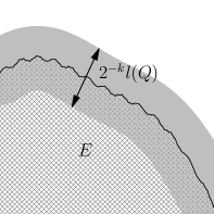
We apply Lemma 2.1 for on at level
to obtain a collection of Calderón–Zygmund cubes
such that
up to a set of Lebesgue measure zero and
|
|
|
By Lemma 2.2, we have
|
|
|
where .
Since
|
|
|
by Lemma 2.1
and
|
|
|
for every ,
it follows that
|
|
|
|
|
|
|
|
|
|
|
|
|
|
|
|
Integrating both sides in and applying Lemma 6.4, we obtain
|
|
|
|
|
|
|
|
We have bounded both summands in 18 which means we can conclude that
|
|
|
where .
∎
7. Examples against weighted -Poincaré inequalities for
and against a larger fractional parameter
In this section,
we prove that the corresponding -versions of the weighted fractional and classical Poincaré inequalities Theorems 4.1 and 6.5 do not hold.
This is motivated by [15, Theorems 2.4 & 2.9] where sub-optimal results were obtained.
More precisely we show that for every cube ,
, , ,
and there is
a Radon measure and a Lipschitz function with
| (19) |
|
|
|
and that for any
, , , ,
and there is
a Radon measure and a Lipschitz function with
| (20) |
|
|
|
We do not know if the condition is necessary.
Moreover, we show that given (and ), the value
(or
respectively)
for the fractional parameter is the best possible for which Theorems 4.1 and 6.5 hold in the following sense.
For any we have the pointwise inequality
for .
Hence, Theorems 4.1 and 6.5 also hold with instead of .
This argument clearly only works for .
And indeed, we show that Theorems 4.1 and 6.5 fail when we replace by with any .
We show this even for the fractional maximal function which is larger than up to a constant.
More precisely, we show that for any , , and
there is a Radon measure
and a Lipschitz function
| (21) |
|
|
|
and that for any , , , and
there is a Radon measure
and a Lipschitz function with
| (22) |
|
|
|
We proceed with the proof of 19, 20, 21 and 22.
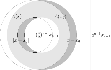
Let
be the cube with center and sidelength .
By translation and dilation it suffices to find a function and a measure which satisfy 19, 20, 21 and 22 on .
Consider the sequence of absolutely continuous measures and Lipschitz functions
|
|
|
with .
Denote
|
|
|
It holds that for .
Thus, for
we have
| (23) |
|
|
|
for any .
Furthermore for any we have
|
|
|
for some dimensional constant
and
|
|
|
Let , and be as specified for 19.
Then
| (24) |
|
|
|
where
.
Choosing large enough, for example
|
|
|
we use 23 and 24 to conclude 19 for .
We use the same sequence of functions and measures to satisfy the remaining inequalities 20, 21 and 22.
In order to find such that satisfies 21,
let , , and be as specified there.
Then we have
| (25) |
|
|
|
where .
Choosing large enough, for example
|
|
|
we use 23 and 25 to conclude 21 for .
In order to find such that satisfies 20 and 22, we first note that
by for example [15, Lemma 3.6],
both and are -weights with
|
|
|
|
|
|
|
|
Since by assumption we have or respectively,
we can apply Corollary 6.3 with
and
and we conclude 20 and 22 from 19 and 21 respectively.