Friedman–Ramanujan functions
in random hyperbolic geometry
and application to spectral gaps

Abstract.

This paper studies the Weil–Petersson measure on the moduli space of compact hyperbolic surfaces of genus $g$. We define “volume functions” associated with arbitrary topological types of closed geodesics, generalising the “volume polynomials” studied by M. Mirzakhani for simple closed geodesics. Our programme is to study the structure of these functions, focusing on their behaviour in the limit $g\longrightarrow+\infty$.

Motivated by J. Friedman’s work on random graphs, we prove that volume functions admit asymptotic expansions to any order in powers of $g^{-1}$, and claim that the coefficients in these expansions belong to a newly-introduced class of functions called “Friedman–Ramanujan functions”. We prove the claim for closed geodesics filling a surface of Euler characteristic $0$ and $-1$. This result is then applied to prove that a random hyperbolic surface has spectral gap $\geq 2/9-\epsilon$ with high probability as $g\rightarrow+\infty$, using the trace method and cancellation properties of Friedman–Ramanujan functions.

1. Introduction

The aim of this article is to develop new geometric tools for the study of random hyperbolic surfaces. Notably, we wish to extend a variety of methods discovered by Mirzakhani [26, 27] allowing the study of simple geodesics to non-simple geodesics.

A compact hyperbolic surface $X$ is a connected, oriented, compact surface, without boundary, equipped with a Riemannian metric of constant curvature $-1$. Its topology is therefore entirely determined by its genus $g\geq 2$. We will be particularly interested in surfaces of large genus. This large-genus limit can be viewed as a large-scale limit, because the area of a compact hyperbolic surface of genus $g$ is $4\pi(g-1)$ by the Gauss–Bonnet formula.

1.1. Random hyperbolic surfaces

Several different models of random hyperbolic surfaces exist [5, 14, 27, 25]. In this article, we will focus solely on the Weil–Petersson model, that consists in equipping the moduli space

$$\mathcal{M}_{g}:=\faktor{\{\text{compact hyperbolic surfaces of genus }g\}}{\text{isometry}}$$

with the probability measure $\mathbb{P}_{g}^{\mathrm{\scriptsize{WP}}}$ obtained by renormalisation of the measure induced by the Weil–Petersson symplectic form on $\mathcal{M}_{g}$. This is a very natural probabilistic setting, in which one can hope to accurately describe typical surfaces.

In her breakthrough articles [26, 27], Mirzakhani developed a toolbox allowing to study the geometry of random hyperbolic surfaces sampled according to the probability $\mathbb{P}_{g}^{\mathrm{\scriptsize{WP}}}$, especially in the large-genus limit. These tools have since then been applied in an ever-growing number of articles, analysing the geometric properties of random surfaces [32, 35, 34, 17], their spectral gap [45, 21, 15, 17] and eigenfunctions [11], as well as the statistics of their length spectrum [28, 44] and Laplacian spectrum [31, 38].

1.2. The spectral gap of a compact hyperbolic surface

While many of the results presented in this article are purely geometric, they are all deeply motivated by an important question in spectral theory, which we shall now present.

The spectral gap of a compact hyperbolic surface is the smallest non-zero eigenvalue $\lambda_{1}>0$ of the (positive) Laplace–Beltrami operator on the surface. Surfaces with a large spectral gap are known to be well-connected [9, 6], fast-mixing for the geodesic flow and random walks [37, 12], and of small diameter [24]. Finding (rich) families of such surfaces has been an objective shared by many, whether in the context of arithmetics and number theory [40, 20], spectral geometry [8], and more recently random hyperbolic geometry [25, 45, 21, 16, 17, 22].

In the large-genus regime, Huber [18] proved that the spectral gap is bounded above by a quantity going to $1/4$ as $g\rightarrow+\infty$ ($1/4$ being the bottom of the spectrum of the hyperbolic plane). The existence of surfaces of large genus with a near-optimal spectral gap was conjectured by Burger–Buser–Dodziuk [8] in the 80’s, and only solved very recently by breakthrough work of Hide–Magee [17] using random covers.

Our aim in this article is to provide new tools and ideas, towards a proof of the fact that hyperbolic surfaces with a near-optimal spectral gap not only exist, but are typical.

Conjecture 1.1.

For any $\epsilon>0$,

$$\lim_{g\rightarrow+\infty}\mathbb{P}_{g}^{\mathrm{\scriptsize{WP}}}\left(\lambda_{1}\geq\frac{1}{4}-\epsilon\right)=1.$$

The literature so far contains two probabilistic spectral gap results in the Weil–Petersson setting. First, Mirzakhani proved in 2013 that random hyperbolic surfaces satisfy $\lambda_{1}>0.002$ with probability going to $1$ as $g\rightarrow+\infty$ [27]. This bound has been vastly improved by two independent teams in 2021, Wu–Xue [45] and Lipnowski–Wright [21], who proved that for all $\epsilon>0$, $\lambda_{1}\geq 3/16-\epsilon$ with probability going to $1$ as $g\rightarrow+\infty$.

The geometric results obtained in this article can be used to obtain the following improved spectral gap result.

Theorem 1.2 (10.1).

For any $\epsilon>0$,

$$\lim_{g\rightarrow+\infty}\mathbb{P}_{g}^{\mathrm{\scriptsize{WP}}}\left(\lambda_{1}\geq\frac{2}{9}-\epsilon\right)=1.$$

In Section 3.4, we explain in detail why the intermediate values $3/16$ and $2/9$ appear naturally, and some of the steps that need to be taken to reach the optimal value $1/4$. The proof relies on the classical trace method, as used in [45, 21], with a major new ingredient developed in this article, which allows us to exhibit non-trivial cancellations.

1.1 is exactly analogous to Alon’s famous conjecture [1] stating that random $d$-regular graphs with $n\gg 1$ vertices typically have a near-optimal spectral gap. It was solved by Friedman in [10], after 20 years of active research. Compact hyperbolic surfaces and regular graphs share a variety of geometric and spectral properties, and the results presented in this article can be seen as analogues of several important steps of Friedman’s proof of Alon’s conjecture.

1.3. Averages of geodesic counting functions

A natural approach to access the geometry and spectrum of random hyperbolic surfaces consists in reducing problems to the study of averages of the form

(1.1) $$\langle F\rangle_{g}^{{\text{all}}}:=\mathbb{E}_{g}^{\mathrm{\scriptsize{WP}}}\Bigg{[}\sum_{\gamma\in\mathcal{P}(X)}F(\ell_{X}(\gamma))\Bigg{]}$$

where

• $\mathcal{P}(X)$ is the set of primitive oriented closed geodesics $\gamma$ on the surface $X$;

• for any closed geodesic $\gamma$ on $X$, $\ell_{X}(\gamma)$ is the length of $\gamma$;

• $F:\mathbb{R}_{\geq 0}\rightarrow\mathbb{R}$ is a measurable function with compact support.

Such averages have been used to obtain geometric results in [27, 28, 32, 34]. Importantly, they appear in trace methods when taking the expectation of the Selberg trace formula, a formula relating the eigenvalues of the Laplacian to the lengths of all closed geodesics on the surface (see Section 3.4).

Unfortunately, the methods developed by Mirzakhani in [26, 27] only allow to study such sums if they are restricted to simple geodesics, i.e. geodesics with no self-intersection:

(1.2) $$\langle F\rangle_{g}^{{\mathrm{s}}}:=\mathbb{E}_{g}^{\mathrm{\scriptsize{WP}}}\Bigg{[}\sum_{\gamma\text{ simple}}F(\ell_{X}(\gamma))\Bigg{]}.$$

This has proven to be very restrictive, and dealing with non-simple closed geodesics is often a challenging aspect of the study of random hyperbolic surfaces [28, 45, 21, 38].

In this paper, we provide new information on the contribution of non-simple geodesics to the average $\langle F\rangle_{g}^{{\mathrm{all}}}$. We hope the tools we develop can be used in various settings.

Remark 1.3.

Wu–Xue proved in [45] that, for any $\eta>0$,

(1.3) $$\langle F\rangle_{g}^{{\mathrm{all}}}=\langle F\rangle_{g}^{{\mathrm{s}}}+\mathcal{O}_{\eta}\left(\frac{1}{g}\,\|F(\ell)\,e^{(1+\eta)\ell}\|_{\infty}\right).$$

As a consequence, at the leading order as $g\rightarrow+\infty$, non-simple geodesics do not contribute to the average $\langle F\rangle_{g}^{{\mathrm{all}}}$. However, we will see in this article that some non-simple geodesics yield contributions decaying like $1/g$ in the average $\langle F\rangle_{g}^{{\mathrm{all}}}$, which means that equation 1.3 cannot be extended past the precision $1/g$.

We explain in Section 3.4 why, in order to reach the optimal spectral gap $1/4-\epsilon$, all computations need to be performed with arbitrary high precision, i.e. with errors decaying in $1/g^{N}$ for arbitrary large $N$. The spectral gap $3/16$ then appears to be the threshold at which a description of the contribution of non-simple geodesics to the average $\langle F\rangle_{g}^{{\mathrm{all}}}$ becomes essential. Our spectral gap result, 1.2, is obtained by entirely analysing the contribution of size $1/g$ of the average $\langle F\rangle_{g}^{{\mathrm{all}}}$.

1.4. Local topological types of geodesics

In order to study the average $\langle F\rangle_{g}^{{\mathrm{all}}}$ where the sum runs over all closed geodesics, we regroup its terms according to what we call the local (topological) type $T$ of $\gamma$. This is done in Section 4, and we refer the reader to Section 2 for the definitions of topological notions appearing below.

The data of a local topological type is given by a pair $[S,\gamma]_{\mathrm{loc}}$, where $S$ is a topological surface with boundary, and $\gamma$ is a closed filling loop on $S$. Several examples are represented in Figure 1. For instance, all simple geodesics are grouped in a local type, given by a simple loop in a cylinder. Another type, which we will describe in detail in this article, is the figure-eight, i.e. geodesics with exactly one self-intersection, represented at the top of Figure 1(b). For this type, $S$ is a pair of pants (a surface of signature $(0,3)$).

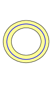
(a) The type “simple”.

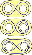
(b) Types filling a pair of pants.

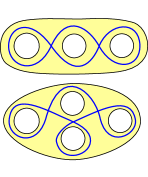
(c) Other types.

Figure 1. A few examples of local types.

Now, we say a closed geodesic $\gamma_{g}$ on a hyperbolic surface $X$ of genus $g$ is of local type $T=[S,\gamma]_{\mathrm{loc}}$ if there exists an embedding $S\rightarrow X$ sending $\gamma$ on $\gamma_{g}$. For a local type $T$ and a measurable function $F:\mathbb{R}_{\geq 0}\rightarrow\mathbb{R}$ with compact support, we define

$$\langle F\rangle_{g}^{{T}}:=\mathbb{E}_{g}^{\mathrm{\scriptsize{WP}}}\Bigg{[}\sum_{\gamma_{g}\text{ of type }T}F(\ell_{X}(\gamma_{g}))\Bigg{]}$$

which allows us to rewrite

(1.4) $$\langle F\rangle_{g}^{{\mathrm{all}}}=\sum_{T\text{ local type}}\langle F\rangle_{g}^{{T}}.$$

Remark 1.4.

The word local is an emphasis on the fact that the notion of local type only depends on the topology of the geodesic itself, and not the way it is embedded in the surface of genus $g$. Notably, all simple closed geodesics form one local type. This notion should not be confused with the notion of topological type, which is often used to refer to mapping-class-group orbits (in Mirzakhani’s work for instance). We prove in 4.11 that the notion of mapping-class-group equivalence is finer than the notion of local equivalence. Hence, every local type can be decomposed as a disjoint union of topological types, which we refer to as its realisations. Realisations correspond to the different ways the pair $(S,\gamma)$ can be embedded in a surface of genus $g$.

1.5. Statement of the main results on the averages

In 5.5, we provide an expression for the averages $\langle F\rangle_{g}^{{T}}$ in terms of Weil–Petersson volumes of moduli spaces of bordered hyperbolic surfaces. We use this expression to prove the following.

Theorem 1.5 (Theorems 5.9 and 5.14).

Let $T=[S,\gamma]_{\mathrm{loc}}$ be a local topological type.

• For any $g\geq 2$, there exists a unique continuous function $V_{g}^{T}:\mathbb{R}_{>0}\rightarrow\mathbb{R}_{\geq 0}$, called volume function, such that, for any measurable function $F$ with compact support,

  $$\langle F\rangle_{g}^{{T}}=\frac{1}{V_{g}}\int_{0}^{+\infty}F(\ell)V_{g}^{T}(\ell)\,\mathrm{d}\ell.$$

• There exists a unique family of continuous functions $(f_{k}^{T})_{k\geq|\chi_{S}|}$ such that, for any $K\geq 0$, any large enough $g$, any $\epsilon>0$,

  (1.5) $$\frac{V_{g}^{T}(\ell)}{V_{g}}=\sum_{k=|\chi_{S}|}^{K}\frac{f_{k}^{T}(\ell)}{g^{k}}+\mathcal{O}_{K,S,\epsilon}^{w}\left(\frac{\exp\left((1+\epsilon)\ell\right)}{g^{K+1}}\right).$$

Remark 1.6.

The notation $\mathcal{O}^{w}\left(\cdot\right)$ is a weak version of the usual Landau notation $\mathcal{O}\left(\cdot\right)$, and introduced in Section 2.1.

1.5 is new in all cases except for the local type “simple”, where it comes as a consequence of [26, 29, 45]. In this case, we know the value of $f_{0}^{\mathrm{s}}(\ell)=\frac{4}{\ell}\sinh^{2}\left(\frac{\ell}{2}\right)$, and this expression is an essential component of many recent results [28, 45, 21, 38].

We highlight the fact that the leading-order term of $\langle F\rangle_{g}^{{T}}$ for the type $T=[S,\gamma]_{\mathrm{loc}}$ decays like $g^{\chi_{S}}$, where $\chi_{S}\leq 0$ is the Euler characteristic of the filled surface $S$. This is the reason why only simple geodesics contribute to the leading term of $\langle F\rangle_{g}^{{\mathrm{all}}}$: for all other local types, $\chi_{S}<0$.

Remark 1.7.

Let us describe the obstacle to the study of non-simple geodesics in Mirzakhani’s work. Mirzakhani’s integration formula [26] allows to write an explicit formula for the average $\langle F\rangle_{g}^{{\mathrm{s}}}$. This is done by considering a random hyperbolic surface $X$ of genus $g$ containing a simple closed geodesic $\gamma$ of length $\ell$, and analysing the topology of the surface $X\setminus\gamma$ obtained by cutting $X$ along the geodesic $\gamma$. Because the geodesic is simple, the result is a (possibly disconnected) hyperbolic surfaces with two geodesic boundary components of length $\ell$.

This unfortunately ceases to be true for non-simple geodesics. In order to remedy this, we rather cut $X$ along the boundary components of the surface $S_{\gamma}$ filled by the non-simple geodesic $\gamma$. This approach was used to a certain extent in [28, 45, 21], but we push it further, which allows us to write a formula for $\langle F\rangle_{g}^{{T}}$ (5.5). The formula is more involved, because it contains an average on all possible hyperbolic metrics on the filled surface $S_{\gamma}$ for which $\gamma$ has length $\ell$.

Example 1.8.

In 5.7, we compute $\langle F\rangle_{g}^{{T}}$ for the type $T=[P,\gamma]_{\mathrm{loc}}$, where $P$ is a pair of pants and $\gamma$ a figure-eight. A metric on the pair of pants $P$ is entirely described by the lengths $\ell_{1},\ell_{2},\ell_{3}$ of its three boundary components. As a consequence, the formula for $\langle F\rangle_{g}^{{T}}$ in this setting takes the form of an integration on the two-dimensional level-set

(1.6) $$\left\{(\ell_{1},\ell_{2},\ell_{3})\in\mathbb{R}_{>0}^{3}\,:\,\cosh\left(\frac{\ell}{2}\right)=2\cosh\left(\frac{\ell_{1}}{2}\right)\cosh\left(\frac{\ell_{2}}{2}\right)+\cosh\left(\frac{\ell_{3}}{2}\right)\right\}$$

which corresponds to the metrics on $P$ for which the length of the figure-eight is exactly $\ell$.

In Section 6, we explain how to adapt 1.5 to the overall average $\langle F\rangle_{g}^{{\mathrm{all}}}$, obtained by summing over all closed geodesics.

Theorem 1.9 (Theorems 6.2 and 6.3).

• There exists a unique continuous function $V_{g}^{\mathrm{all}}:\mathbb{R}_{>0}\rightarrow\mathbb{R}_{\geq 0}$ such that, for any measurable function $F$ with compact support,

  $$\langle F\rangle_{g}^{{\mathrm{all}}}=\frac{1}{V_{g}}\int_{0}^{+\infty}F(\ell)V_{g}^{\mathrm{all}}(\ell)\,\mathrm{d}\ell.$$

• There exists a unique family of continuous functions $(f_{k}^{\mathrm{all}})_{k\geq 0}$ such that, for any $A\geq 1$, $K\geq 0$, $\epsilon>0$, and any large enough $g$,

  (1.7) $$\frac{V_{g}^{\mathrm{all}}(\ell)}{V_{g}}\mathds{1}_{[0,A\log(g)]}(\ell)=\sum_{k=0}^{K}\frac{f_{k}^{\mathrm{all}}(\ell)}{g^{k}}\mathds{1}_{[0,A\log(g)]}(\ell)+\mathcal{O}_{\epsilon,K,A}^{w}\left(\frac{\exp{(1+\epsilon)\ell}}{g^{K+1}}\right).$$

Remark 1.10.

The indicator function in equation 1.7 is used to reduce the number of local topological types that need to be summed when computing $\langle F\rangle_{g}^{{\mathrm{all}}}$. Indeed, if we do not assume that we only look at geodesics of length $\leq A\log(g)$, we a priori need to take into account the geodesics filling the whole surface of genus $g$, for instance.

Now that we know that the averages $\langle F\rangle_{g}^{{T}}$ and $\langle F\rangle_{g}^{{\mathrm{all}}}$ admit asymptotic expansions in powers of $1/g$, we shall be concerned with the form of the coefficients $(f_{k}^{T})_{k\geq 0}$ and $(f_{k}^{\mathrm{all}})_{k\geq 0}$ appearing in these expansions.

1.6. Friedman–Ramanujan functions

An essential step in Friedman’s proof of Alon’s conjecture is the introduction of a notion of Ramanujan functions [10, Section 7]. We adapt this notion to the context of random hyperbolic geometry. We then show that this class of functions arises naturally when studying the lengths of geodesics on random hyperbolic surfaces, and its relevance to the spectral gap problem.

Definition 1.11 (3.1).

A continuous function $f:\mathbb{R}_{>0}\rightarrow\mathbb{C}$ is said to be a Friedman–Ramanujan function if there exists a polynomial function $p$ and a constant $c>0$ such that

$$f(\ell)=p(\ell)\,e^{\ell}+\mathcal{O}\left((\ell+1)^{c}e^{\frac{\ell}{2}}\right).$$

We denote as $\mathcal{F}$ the class of Friedman–Ramanujan functions, and as $\mathcal{R}$ the subset of Friedman–Ramanujan function for which $p=0$. We similarly define a notion of Friedman–Ramanujan function in the weak sense using the weaker $\mathcal{O}^{w}\left(\cdot\right)$.

This is a natural adaptation of Friedman’s definition of Ramanujan functions for $d$-regular graphs, namely functions $f:\mathbb{Z}_{>0}\rightarrow\mathbb{C}$ such that

$$f(k)=p(k)\,(d-1)^{k}+\mathcal{O}\left(k^{c}(d-1)^{\frac{k}{2}}\right)$$

for a polynomial function $p$ and a constant $c>0$. The quantities $e^{\ell}$ and $(d-1)^{k}$ are the growth-rate of balls in the hyperbolic plane and the $d$-regular tree respectively.

Remark 1.12.

The name “Ramanujan” was chosen by Friedman in relationship to the breakthrough work by Lubotzky–Phillips–Sarnak [23], in which the authors prove the existence of large $d$-regular graphs with an optimal spectral gap (such graphs were called Ramanujan graphs due to the use of the Ramanujan conjecture in [23]). We have chosen the name “Friedman–Ramanujan” with the wish to both maintain the link with the original article that inspired this work and emphasise Friedman’s impressive contribution to the study of random $d$-regular graphs.

Remark 1.13.

An alternative way to understand the definition of Friedman–Ramanujan function and its relation to the spectral gap problem is to look at the prime number theorem with error terms, proven by Huber [18] (see also [7, Theorem 9.6.1]). This theorem states that, for a fixed hyperbolic surface $X$ and a large $\ell$,

$$N_{X}(\ell):=\#\{\gamma:\ell_{X}(\gamma)\leq\ell\}=\operatorname{li}(e^{\ell})+\sum_{j:0<\lambda_{j}<\frac{3}{16}}\operatorname{li}\big{(}e^{\left(\frac{1}{2}+\sqrt{\frac{1}{4}-\lambda_{j}}\right)\,\ell}\big{)}+\mathcal{O}\left(\frac{e^{\frac{3}{4}\ell}}{\ell}\right)$$

where $\operatorname{li}(x):=\int_{2}^{x}\frac{\,\mathrm{d}\tau}{\log\tau}\sim x/\log(x)$. The leading term $\operatorname{li}(e^{\ell})\sim e^{\ell}/\ell$ comes from the eigenvalue $\lambda_{0}=0$. We observe that small eigenvalues (or at least the ones smaller than $3/16$) correspond to subdominant contributions to $N_{X}(\ell)$. The exponent gap in the definition of Friedman–Ramanujan functions, between the exponent $e^{\ell}$ in the main term and the exponent $e^{\ell/2}$ in the remainder, corresponds exactly to the gap between the trivial eigenvalue $0$ and the optimal spectral gap $1/4$.

1.7. Link between Friedman–Ramanujan functions and spectral gaps

The motivation behind the introduction of Friedman–Ramanujan functions is that one can exhibit cancellations in the Selberg trace formula thanks to their structure. We discuss this relationship in Section 3.4. It motivates the following objective.

Objective (FR).

Let $T$ be a local type, and $s_{T}=1$ if $T$ is “simple” and $0$ otherwise. Prove that, for any $k\geq 0$, the function $\ell\mapsto\ell^{s_{T}}f_{k}^{T}(\ell)$ is a Friedman–Ramanujan function in the weak sense.

For the local type “simple”, we recall that we know that $f_{0}^{\mathrm{s}}(\ell)=\frac{4}{\ell}\sinh^{2}\left(\frac{\ell}{2}\right)$, where the function $\ell\mapsto 4\sinh^{2}\left(\frac{\ell}{2}\right)$ is a Friedman–Ramanujan function. For higher-order terms in $\langle F\rangle_{g}^{{\mathrm{s}}}$, we show in 3.3 that our previous work [2] implies our claim for the type “simple”. In this article, we prove it for the following local types.

Theorem 1.14.

For any local type $T$ filling a surface of Euler characteristic $-1$, all functions $(f_{k}^{T})_{k\geq 0}$ are Friedman–Ramanujan in the weak sense.

Surfaces of Euler characteristic $-1$ are the pair of pants and the once-holed torus. The proofs are quite technical, notably due to the difficulties hinted at in 1.7. They are presented in Sections 7 (for the figure-eight filling a pair of pants) and 8 (for all other loops filling a pair of pants or once-holed torus). Because the expansion in 1.5 starts with the term $k=|\chi_{S}|$, 1.14 has the following immediate consequence.

Corollary 1.15.

For any local type $T$, the function $\ell\mapsto\ell^{s_{T}}f_{k}^{T}(\ell)$ is Friedman–Ramanujan in the weak sense for $k=0$ and $1$.

This result is the key ingredient to the proof of 1.2. We hope to fulfil Objective (FR) for any local type in a forthcoming paper. The analysis presented in Section 3.4 explains why it would be a significant step towards a proof of 1.1.

1.8. The challenge of tangles

Another striking demonstration of the intimate relationship between Friedman–Ramanujan functions and the spectral gap problem can be found in our proof of the following statement.

Theorem 1.16 (9.1).

The function $\ell\mapsto\ell f_{1}^{\mathrm{all}}(\ell)$ is not a Friedman–Ramanujan function in the weak sense.

This might seem surprising, because 1.15 implies that $\ell\mapsto\ell f_{1}^{\mathrm{all}}(\ell)$ is a countable sum of Friedman–Ramanujan functions in the weak sense, and this condition is stable by linear combination. The proof of this result consists in proving that, if the counting functions are Friedman–Ramanujan, then we can obtain quantitative information on the spectral gap.

Lemma 1.17 (9.6).

If $\ell\mapsto\ell f_{1}^{\mathrm{all}}(\ell)$ is a Friedman–Ramanujan function in the weak sense, then for small $\delta>0$ and large enough $g$,

(1.8) $$\mathbb{P}_{g}^{\mathrm{\scriptsize{WP}}}\left(\delta<\lambda_{1}<\frac{5}{72}\right)=\mathcal{O}_{\delta}\left(\frac{1}{g^{5/4}}\right).$$

The contradiction then arises from the following estimate on the probability for a surface to have a small eigenvalue.

Theorem 1.18 (9.2).

There exists $c_{1}>0$ and $c_{2}>0$ such that, for small enough $a>0$ and large enough $g$,

$$c_{1}\frac{a^{2}}{g}\leq\mathbb{P}_{g}^{\mathrm{\scriptsize{WP}}}\left(\lambda_{1}\leq a\right)\leq c_{2}\frac{a}{g}\cdot$$

In particular the rate of growth $g^{-5/4}$ in 1.17 is too fast. 1.18 is obtained by observing that, for a small $a>0$, the probability for a random surface to contain a once-holed torus with a boundary of length $\leq a$ is roughly $a^{2}/g$. By the min-max principle, if a surface contains such a piece, then $\lambda_{1}\leq a$.

More generally, embedded subsurfaces with a short boundary are linked to the presence of small eigenvalues, because in this case the surface is poorly connected [9, 6]. We call such subsurfaces tangles – this notion appears in [32, 21].

The value $3/16$ is the threshold at which tangles start to manifest, because their probability is of size $1/g$. In order to go past $3/16$, we need to remove tangles. In Friedman’s proof of the Alon conjecture, the presence of tangles is a significant challenge: those issues are explained in [10, Section 2] and are the motivation for introducing a notion of selective trace.

In our proof of 1.2, we remove tangles using an inclusion-exclusion argument similar to the one use by Lipnowski–Wright in [21]. Our notion of tangle-freeness is close to the notion defined by Bordenave in his proof of Friedman’s theorem [4], and studied by the second author and Thomas in [32]. Unfortunately, our inclusion-exclusion argument relies on a tedious topological enumeration, much more complex than the one in [21]. We aim to present a more general method to remove tangles, based on Friedman’s approach, in an upcoming article. We believe that proving Objective (FR) in all generality, and extending Friedman’s tangle-removal techniques to hyperbolic surfaces, will allow us to conclude to a proof of 1.1.

Acknowledgements

The authors would like to express their gratitude to Joel Friedman, for explaining his proof of Alon’s conjecture to us in detail, which lead to significant advances in our project. We would also like to thank Michael Lipnowski and Alex Wright for sharing their insight on the spectral gap problem. We are grateful to Nir Avni and Steve Zelditch for the conference they organised in Northwestern University, where we met Joel Friedman and presented some of these results for the first time.

This research was partly funded by the guest program of the Max-Planck Institute for Mathematics during the year 2021-2022, the EPSRC grant EP/W007010/1 since 2022, as well as the prize L’Oréal-UNESCO Young Talents France for Women in Science.

2. Preliminaries

In this section, we introduce many objects relevant to this article, for the sake of clarity and self-containment. For a more detailed exposition of these notions, we refer the reader to [7] for hyperbolic geometry, and [43, 30] for the theory of random hyperbolic surfaces.

2.1. Notations

For two quantities $F_{1},F_{2}$, we write $F_{1}=\mathcal{O}\left(F_{2}\right)$ if there exists a constant $C>0$ such that $|F_{1}|\leq CF_{2}$ for any choice of parameters within the allowed ranges. If the constant depends on a parameter $\alpha$, we write $F_{1}=\mathcal{O}_{\alpha}\left(F_{2}\right)$.

For a Borel measure $\mu$ on $\mathbb{R}^{n}$ and a positive measurable function $F:\mathbb{R}^{n}\rightarrow\mathbb{R}_{>0}$, we say that $\mu=\mathcal{O}^{w}\left(F\right)$ if $\mu$ is bounded by $F$ in a weak sense, i.e. if there exists a constant $C>0$ such that the total mass of $|\mu|/F$ is smaller than $C$ for any choice of parameters. If $C$ depends on a parameter $\alpha$, we rather write $\mu=\mathcal{O}_{\alpha}^{w}\left(F\right)$.

2.2. Hyperbolic geometry and closed geodesics

2.2.1. Compact and bordered surfaces

All surfaces in this article are assumed to be oriented, connected and of finite type (with a finitely generated fundamental group).

A compact hyperbolic surface $X$ is a closed surface equipped with a Riemannian metric of constant curvature $-1$. The topology of $X$ is therefore entirely determined by its genus $g\geq 2$. By the Gauss–Bonnet formula, $X$ has finite area, equal to $2\pi|\chi_{X}|$, where $\chi_{X}=2-2g<0$ is the Euler characteristic of $X$, which shall be denoted as $\chi_{g}$.

The study of compact hyperbolic surfaces is the core focus of this article. However, in doing so, we will need to cut these surfaces along some simple closed geodesics – which shall lead us to consider surfaces with a geodesic boundary. A bordered hyperbolic surface is a surface equipped with a Riemannian metric of curvature $-1$, with a (finite) set of boundary components, labelled $\{1,\ldots,n\}$, which are either closed geodesics or cusps (which we will abusively refer to as components of length $0$). The signature of $X$ is the pair $(g,n)$, where $g$ is its genus. The Gauss–Bonnet formula extends to this setting, with $\chi_{X}=2-2g-n$. The case $n=0$ corresponds to the compact case above.

2.2.2. Primitive closed geodesics

A loop on $X$ is a continuous map $\gamma:[0,1]\rightarrow X$ such that $\gamma(0)=\gamma(1)$. Two loops $\gamma_{0}$ and $\gamma_{1}$ are said to be (freely) homotopic if there exists a continuous map $h:[0,1]\times[0,1]\rightarrow X$ such that $h_{|\{0\}\times[0,1]}=\gamma_{0}$ and $h_{|\{1\}\times[0,1]}=\gamma_{1}$; we then write $\gamma_{0}\,\raisebox{-2.84526pt}{$\mathrel{\ensurestackMath{\stackengine{-.2pt}{\scriptscriptstyle\mathrm{h}}{\sim}{O}{c}{F}{F}{S}}}$}\,\gamma_{1}$. We say the loop $\gamma$ is non-primitive if there exists an integer $m\geq 2$ and a loop $\gamma_{0}$ such that $\gamma\,\raisebox{-2.84526pt}{$\mathrel{\ensurestackMath{\stackengine{-.2pt}{\scriptscriptstyle\mathrm{h}}{\sim}{O}{c}{F}{F}{S}}}$}\,\gamma_{0}^{m}$; otherwise, $\gamma$ is primitive. A loop is called essential if it is neither contractible nor homotopic to a boundary component or a cusp of $X$ (the second condition only matters if $X$ is a bordered surface).

We denote as $\mathcal{P}(X)$ the set of homotopy-classes of primitive essential loops on $X$. It can alternatively be seen as the set of primitive (oriented) closed geodesics on $X$, because each homotopy class in $\mathcal{P}(X)$ contains a unique geodesic representative. For $\gamma\in\mathcal{P}(X)$, we denote as $\ell_{X}(\gamma)$ the length of the geodesic representative in the homotopy class $\gamma$.

In the following, we will often abusively refer to elements of $\mathcal{P}(X)$ as homotopy classes, loops, or closed geodesics; in the latter two cases we will always talk about them up to homotopy. In particular, we say that two elements $\gamma_{0}$ and $\gamma_{1}$ of $\mathcal{P}(X)$ are distinct (and denote $\gamma_{0}\neq\gamma_{1}$) if $\gamma_{0}$ is not homotopic to $\gamma_{1}$. These elements are called disjoint if $\gamma_{0}\neq\gamma_{1}$, $\gamma_{0}\neq\gamma_{1}^{-1}$, and if the homotopy classes $\gamma_{0}$, $\gamma_{1}$ admit representatives which have no intersections. An element of $\mathcal{P}(X)$ is simple if it admits a representative with no self-intersections (which implies that the geodesic representative does). A multi-curve is an ordered family $(\gamma_{1},\ldots,\gamma_{k})$ of disjoint simple elements of $\mathcal{P}(X)$; taking the geodesic representative of each homotopy class in this family yields a family of simple, disjoint geodesics on $X$ (i.e. the geodesics have no self-intersections and no mutual intersections).

2.2.3. Geodesic counting

The set of primitive closed geodesics on a hyperbolic surface is discrete, and we shall need to count geodesics of a bounded length. Several counting arguments will appear in this article, the simplest being the following.

Lemma 2.1.

Let $X$ be a hyperbolic surface, compact or bordered. For any $L>0$,

$$\#\{\gamma\in\mathcal{P}(X)\,|\,\ell_{X}(\gamma)\leq L\}\leq 205\,|\chi_{X}|\,e^{L}.$$

Proof.

First, if $X$ is compact of genus $g$, then by [7, Theorem 4.1.6 and Lemma 6.6.4],

$$\#\{\gamma\text{ primitive geodesic }|\,\ell_{X}(\gamma)\leq L\}\leq 3g-3+(g-1)\,e^{L+6}$$

which implies the result, because $|\chi_{X}|=2g-2$.

Following the proof of [28, Proposition 4.5], we extend the result to surfaces with a boundary, by doubling the surface: we take two copies of the surface $X$ and glue them along their matching boundary components. We obtain a compact surface $X^{\prime}$, of Euler characteristic $2\chi_{X}$ by additivity of the Euler characteristic. Each primitive closed geodesic on $X$ can be sent injectively on two primitive closed geodesics on $X^{\prime}$ of the same length, and hence the number of primitive closed geodesics $\leq L$ on $X$ is smaller than half the number of primitive closed geodesics on $X^{\prime}$. ∎

2.2.4. Filling geodesics and Wu–Xue’s improved geodesic counting

When studying a closed geodesic $\gamma$ on a surface $X$, it is often very convenient to introduce a subsurface of $X$ that is filled by $\gamma$ in the following sense.

Definition 2.2.

Let $S$ be a topological surface, possibly with a boundary. We say a loop $\gamma$ on $S$ fills the surface $S$ if each connected component of $S\setminus\gamma$ is either contractible or an annular region around a boundary component of $S$.

For a fixed $S$, one can wonder how many geodesics of length $\leq L$ fill $S$. An impressive counting result on this quantity was obtained by Wu–Xue in [45].

Theorem 2.3.

For any $\eta>0$, any topological surface $S$ with boundary, there exists a constant $C_{S,\eta}>0$ such that, for any hyperbolic metric $Y$ on $S$, any $L>0$,

$$\#\{\gamma\text{ primitive loops filling }S\,:\,\ell_{Y}(\gamma)\leq L\}\leq C_{S,\eta}\exp\left(L-\frac{1-\eta}{2}\,\ell_{Y}(\partial S)\right).$$

This result is an improvement of the naive bound from 2.1, thanks to the decaying properties of the term $\exp((1-\eta)\ell_{Y}(\partial S)/2)$. It is a central part of Wu–Xue’s proof that typical surfaces have a spectral gap at least $3/16-\epsilon$.

2.3. Random hyperbolic surfaces

Let $g\geq 2$. In this article, we sample random hyperbolic surfaces of genus $g$ according to the Weil–Petersson probabilistic setting, which we shall now introduce briefly.

2.3.1. The moduli space

We sample our random surfaces in the moduli space

$$\mathcal{M}_{g}:=\{\text{compact hyperbolic surfaces }X\text{ of genus }g\}\diagup\text{isometry}.$$

In order to study the moduli space, it is very convenient to introduce its universal covering, the Teichmüller space $\mathcal{T}_{g}$, which can be seen as the set of marked hyperbolic surfaces. More precisely, we fix a surface $S_{g}$ of genus $g$, which we call the base surface. Then,

$$\mathcal{T}_{g}=\left\{(X,\phi),\quad\parbox{176.407pt}{$X$ compact hyperbolic surface \\ $\phi:S_{g}\rightarrow X$ positive homeomorphism}\right\}\diagup\,\raisebox{-2.84526pt}{$\mathrel{\ensurestackMath{\stackengine{-.2pt}{\scriptscriptstyle\mathrm{Teich}}{\sim}{O}{c}{F}{F}{S}}}$}\,$$

where the quotient is defined by saying that $(X_{1},\phi_{1})\,\raisebox{-2.84526pt}{$\mathrel{\ensurestackMath{\stackengine{-.2pt}{\scriptscriptstyle\mathrm{Teich}}{\sim}{O}{c}{F}{F}{S}}}$}\,(X_{2},\phi_{2})$ if there exists an isometry $m:X_{1}\rightarrow X_{2}$ such that $m\circ\phi_{1}$ and $\phi_{2}$ are isotopic. The mapping class group

$$\mathrm{MCG}_{g}:=\{\text{positive homeomorphisms }\psi:S_{g}\rightarrow S_{g}\}\diagup\text{isotopy}$$

naturally acts on the Teichmüller space by precomposition of the marking:

$$\psi\cdot(X,\phi):=(X,\phi\circ\psi^{-1}).$$

Then the moduli space, as the space of “unmarked” hyperbolic surfaces, is obtained by forgetting the marking, i.e.

$$\mathcal{M}_{g}=\mathcal{T}_{g}\diagup\mathrm{MCG}_{g}.$$

2.3.2. Length functions

Closed geodesics on a marked surface $(X,\phi)$ are in a natural correspondence with homotopy-classes of loops on the base surface $S_{g}$, thanks to the marking $\phi:S_{g}\rightarrow X$. Indeed, if we denote as $\mathcal{P}_{g}:=\mathcal{P}(S_{g})$ the set of homotopy classes of primitive loops on $S_{g}$, then for any $(X,\phi)\in\mathcal{T}_{g}$, the marking $\phi:S_{g}\rightarrow X$ provides a one-to-one correspondence between $\mathcal{P}_{g}$ and $\mathcal{P}(X)$. We can therefore define, for a $(X,\phi)\in\mathcal{T}_{g}$ and $\gamma\in\mathcal{P}_{g}$, the length $\ell_{(X,\phi)}(\gamma):=\ell_{X}(\phi(\gamma))$ to be the length of the geodesic representative in the homotopy class $\phi(\gamma)$ on $X$. Note that we will often abusively remove the mention of the marking, so that we will sometimes write $\ell_{X}(\gamma)$ for a $X\in\mathcal{T}_{g}$ and $\gamma\in\mathcal{P}_{g}$; in this case, it is implied that the overall quantity that we are studying is $\mathrm{MCG}_{g}$-invariant, so that the marking does not need to be emphasised.

The mapping class group $\mathrm{MCG}_{g}$ naturally acts on loops on the base surface $S_{g}$, by composition $\psi\cdot\gamma:=\psi\circ\gamma$. The orbit of $\gamma$ for this action is denoted as $\mathrm{Orb}(\gamma)$, and the stabilisator $\mathrm{Stab}(\gamma)$. We write $\gamma_{1}\,\raisebox{-2.84526pt}{$\mathrel{\ensurestackMath{\stackengine{-.2pt}{\scriptscriptstyle\mathrm{MCG}}{\sim}{O}{c}{F}{F}{S}}}$}\,\gamma_{2}$ if there exists a $\psi\in\mathrm{MCG}_{g}$ such that $\psi\cdot\gamma_{1}=\gamma_{2}$, in which case $\gamma_{1}$ and $\gamma_{2}$ are said to have the same (global) topological type. This action also extends naturally to an action on multi-curves, or on families of loops, and we use the same notations in these cases.

Remark 2.4.

In most papers of the field, e.g. [26, 27, 28, 45, 21, 38], geodesics are considered to be non-oriented, and orbits and stabilisers are defined for non-oriented loops, and therefore different from ours. Here, we choose to consider all loops and multi-curves to be oriented, because the Selberg trace formula classically runs over all oriented geodesics. We believe this convention to make a few discussions about constants appearing in formulas slightly simpler.

2.3.3. Weil–Petersson form and probability measure

The Weil–Petersson form $\omega_{g}^{\mathrm{WP}}$ is a natural symplectic structure on the Teichmüller space $\mathcal{T}_{g}$, which is invariant by the action of $\mathrm{MCG}_{g}$ and therefore descends to the moduli space $\mathcal{M}_{g}$ [41].

A pair of pants is a surface of signature $(0,3)$, and a pair of pants decomposition of $S_{g}$ is a multi-curve $(\gamma_{1},\ldots,\gamma_{3g-3})$, that cuts $S_{g}$ into $2g-2$ pairs of pants. For $(X,\phi)\in\mathcal{T}_{g}$, after homotopy, this multi-curve is sent to a decomposition of $X$ in hyperbolic pairs of pants, with boundary lengths and twists $(\ell_{i},\tau_{i})_{1\leq i\leq 3g-3}$. These numbers, called Fenchel–Nielsen parameters, are global coordinates on the Teichmüller space $\mathcal{T}_{g}\simeq(\mathbb{R}_{>0}\times\mathbb{R})^{3g-3}$. Wolpert proved in [42] that Fenchel–Nielsen coordinates are symplectic coordinates for the Weil–Petersson form:

(2.1) $$\omega_{g}^{\mathrm{WP}}=\sum_{i=1}^{3g-3}\,\mathrm{d}\ell_{i}\wedge\,\mathrm{d}\tau_{i}.$$

As any symplectic form does, the Weil–Petersson form induces a volume form on the Teichmüller space and moduli space, defined by $\operatorname{Vol}_{g}^{\mathrm{WP}}:=(\omega_{g}^{\mathrm{WP}})^{\wedge(3g-3)}/(3g-3)!$. This volume form is the Lebesgue measure $\,\mathrm{d}\ell_{1}\,\mathrm{d}\tau_{1}\ldots\,\mathrm{d}\ell_{3g-3}\,\mathrm{d}\tau_{3g-3}$ in Fenchel–Nielsen parameters. The total mass of the moduli space is finite, and we shall denote it as $V_{g}$. As a consequence, we can renormalise the Weil–Petersson volume form, and hence equip the moduli space $\mathcal{M}_{g}$ with the Weil–Petersson probability measure

$$\mathbb{P}_{g}^{\mathrm{WP}}:=\frac{1}{V_{g}}\operatorname{Vol}_{g}^{\mathrm{WP}}.$$

2.3.4. Spaces of bordered surfaces

As mentioned in Section 2.2.1, we will need to consider not only compact surfaces but also bordered surfaces for the purposes of this article. The definitions above naturally extend to define, for $(g,n)$ such that $2g-2+n>0$ and $n>0$, $\mathbf{x}=(x_{1},\ldots,x_{n})\in\mathbb{R}_{\geq 0}^{n}$, the moduli space

$$\mathcal{M}_{g,n}(\mathbf{x}):=\left\{\parbox{233.3125pt}{bordered hyperbolic surface $X$ of signature $(g,n)$ \\ $\forall i$, the $i$-th component of $X$ has length $x_{i}$}\right\}\diagup\text{isometry}$$

where the quotient is over positive isometries that preserve each individual boundary component set-wise. Similarly, we fix a base surface $S_{g,n}$ of signature $(g,n)$, which allows us to write

$$\mathcal{M}_{g,n}(\mathbf{x})=\mathcal{T}_{g,n}(\mathbf{x})\diagup\mathrm{MCG}_{g,n},$$

where the Teichmüller space $\mathcal{T}_{g,n}(\mathbf{x})$ is the space of marked bordered hyperbolic surfaces and $\mathrm{MCG}_{g,n}$ is the mapping class group of $S_{g,n}$ (considering only homeomorphisms fixing each individual boundary component of $S_{g,n}$ set-wise).

In this more general setting, there is also a Weil–Petersson symplectic form $\omega_{g,n,\mathbf{x}}^{\mathrm{WP}}$ defined on both $\mathcal{M}_{g,n}(\mathbf{x})$ and $\mathcal{T}_{g,n}(\mathbf{x})$, which has the same expression (2.1) for any pair of pants decomposition $(\gamma_{1},\ldots,\gamma_{3g-3+n})$ of the base surface $S_{g,n}$. The volume form induced by this symplectic structure is denoted as $\operatorname{Vol}_{g,n,\mathbf{x}}^{\mathrm{WP}}$. The quantity $V_{g,n}(\mathbf{x})$ denotes the total mass of the moduli space, with the exception that $V_{1,1}(x):=\frac{1}{2}\operatorname{Vol}_{1,1,x}(\mathcal{M}_{1,1}(x))$ (this symmetry constant $1/2$ reflects the existence of an involution symmetry for every once-holed torus with boundary – see [43, Section 2.8]). We shall omit the mention of the length-vector $\mathbf{x}$ whenever it is equal to $(0,\ldots,0)$, i.e. when all boundary components are cusps, hence making sense of the notations $\mathcal{M}_{g,n}$, $\mathcal{T}_{g,n}$ and $V_{g,n}$.

2.4. Mirzakhani’s integration formula

Let $g\geq 2$, $k\geq 1$ and $\Gamma=(\gamma_{1},\ldots,\gamma_{k})$ be a multi-curve on the base surface $S_{g}$. For a measurable function $F:\mathbb{R}_{\geq 0}^{k}\rightarrow\mathbb{R}$ with compact support (or decaying fast enough) and an element $X\in\mathcal{M}_{g}$, we define

(2.2) $$F^{\Gamma}(X):=\sum_{(\alpha_{1},\ldots,\alpha_{k})\in\mathrm{Orb}(\Gamma)}F(\ell_{X}(\alpha_{1}),\ldots,\ell_{X}(\alpha_{k})).$$

For any $(X,\phi)\in\mathcal{T}_{g}$, cutting the surface $X$ along the multi-geodesic representative of the multi-curve $\phi(\Gamma)$ yields a family of $q\geq 1$ bordered hyperbolic surfaces. We pick a numbering for these surfaces, and for $1\leq i\leq q$ denote as $(g_{i},n_{i})$ the signature of the $i$-th surface. If $\mathbf{x}\in\mathbb{R}_{\geq 0}^{k}$ is a list of values for the respective lengths of $\phi(\gamma_{1}),\ldots,\phi(\gamma_{k})$ on $X$, then for every $i$, the lengths of the boundary components of the $i$-th surface is a vector $\mathbf{x}^{(i)}\in\mathbb{R}_{\geq 0}^{n_{i}}$. Note that each component of $\mathbf{x}$ is present exactly twice in the overall family of vectors $(\mathbf{x}^{(i)})_{1\leq i\leq q}$, and $\sum_{i=1}^{q}n_{i}=2k$, because the $\phi(\gamma_{i})$s each have two sides. Then, Mirzakhani’s integration formula reads as follows.

Theorem 2.5 ([26]).

For $g\geq 3$, the integral of $F^{\Gamma}$ over the moduli space can be computed as

(2.3) $$\int_{\mathcal{M}_{g}}F^{\Gamma}(X)\,\mathrm{d}\operatorname{Vol}_{g}^{\mathrm{WP}}(X)=\int_{\mathbb{R}_{\geq 0}^{k}}F(\mathbf{x})\,\prod_{i=1}^{q}V_{g_{i},n_{i}}(\mathbf{x}^{(i)})\,\prod_{i=1}^{k}x_{i}\,\mathrm{d}x_{i}.$$

Example 2.6.

Let us demonstrate how we can use 2.5 to compute the average $\langle F\rangle_{g}^{{\mathrm{s}}}$, defined by summing over all simple geodesics (see equation 1.2). We define the following loops on the base surface $S_{g}$.

• $\gamma_{0}$ is a simple loop such that $S_{g}\setminus\gamma_{0}$ is connected (we call such a loop a non-separating loop).

• For $1\leq i\leq g-1$, $\gamma_{i}$ is a simple loop such that $S_{g}\setminus\gamma_{i}$ has two connected components: on the left side of $\gamma$, a surface of signature $(i,1)$, and on the right side, a surface of signature $(g-i,1)$.

Then, any simple (oriented) loop on $S_{g}$ lies in the orbit of exactly one $\gamma_{i}$ for a $i\geq 0$. Hence,

$$\langle F\rangle_{g}^{{\mathrm{s}}}=\mathbb{E}_{g}^{\mathrm{\scriptsize{WP}}}\Bigg{[}\sum_{\gamma\text{ simple}}F(\ell_{X}(\gamma))\Bigg{]}=\frac{1}{V_{g}}\sum_{i=0}^{g-1}\int_{\mathcal{M}_{g}}F^{\gamma_{i}}(X)\,\mathrm{d}\operatorname{Vol}_{g}^{\mathrm{WP}}(X).$$

We then apply Mirzakhani’s integration formula to each of these multi-curves, to conclude that

$$\langle F\rangle_{g}^{{\mathrm{s}}}=\frac{1}{V_{g}}\int_{0}^{+\infty}F(\ell)\left(V_{g-1,2}(\ell,\ell)+\sum_{i=1}^{g-1}V_{i,1}(\ell)V_{g-i,1}(\ell)\right)\ell\,\mathrm{d}\ell.$$

Remark 2.7.

2.5 appears in the literature in various forms, and there is always a symmetry factor $c_{\Gamma}\in(0,1]$ in the right hand side of equation 2.3 [26, 27, 43, 45, 21]. No such constant appears for us due to the combination of the following choices.

• A factor $2^{-M(\Gamma)}$, where $M(\Gamma)$ is the number of components of $S_{g}\setminus\Gamma$ that are of signature $(1,1)$, is removed thanks to our convention $V_{1,1}(x):=\frac{1}{2}\operatorname{Vol}_{1,1,x}^{\mathrm{WP}}(\mathcal{M}_{1,1}(x))$.

• There is often a symmetry factor $1/\mathrm{Sym}(\Gamma)$, which varies throughout literature depending on the conventions that are adopted. For instance, in [26], $\mathrm{Sym}(\Gamma)$ is said to be the index of the subgroup $\bigcap_{i=1}^{k}\mathrm{Stab}(\gamma_{i})$ of $\mathrm{Stab}(\Gamma)$. The reason for this discrepancy is that, in [26], the function $F^{\Gamma}$ is defined by averaging a function $F$ that is invariant by permutations, and hence, when $\Gamma$ has non-trivial symmetries, several terms in the function $F^{\Gamma}$ are systematically identical.

• Additional factors, depending on the symmetries of $\Gamma$ with respect to changing orientations of some of its components, appear in [43, 45, 21]. They come from the fact that the multi-curves are usually considered to be non-oriented, as opposed to our convention (see 2.4, and 2.8 below).

• The presence of an additional factor $1/2$ whenever $g=2$, mentioned in [43], due to the existence of the hyper-elliptic involution for surfaces of genus $2$, is the reason why we assume that $g\geq 3$.

Remark 2.8.

In their proof of the $3/16-\epsilon$ spectral gap result, both teams [45, 21] rely heavily on the presence of a factor $1/2$ in the right hand side of equation 2.3, whenever we apply 2.5 to a single simple non-separating closed geodesic $\gamma$. This argument is reproduced in Section 3.4.4. The distinction here comes from the fact that $\gamma$ is non-oriented for them, and oriented for us. We can compare the two formulas by observing that

$$\sum_{\gamma\text{ non-oriented}}F(\ell_{X}(\gamma))=\frac{1}{2}\sum_{\gamma\text{ oriented}}F(\ell_{X}(\gamma)).$$

Contrarily, we do not expect our new approach to the $1/4$ conjecture to require much knowledge on the constants appearing (or not) in 2.5.

2.5. Estimates on Weil–Petersson volumes

2.5 allows us to reduce the question of estimating $\mathbb{E}_{g}^{\mathrm{\scriptsize{WP}}}[F^{\Gamma}]$ to the study of the Weil–Petersson volumes. Many estimates are known on the behaviour of $V_{g,n}=V_{g,n}(0,\ldots,0)$ in terms of $g$ and $n$ [27, 29, 28, 34]. We shall use several of these estimates throughout this article, referencing them carefully.

In terms of asymptotic expansions, Mirzakhani and Zograf have proved in [29] the existence of coefficients $(a_{k,n})_{k>0}$ and $(b_{k,n})_{k>0}$, for $n\geq 0$, such that for $K\geq 0$,

(2.4) $$\frac{V_{g-1,n+2}}{V_{g,n}}=1+\sum_{k=1}^{K}\frac{a_{k,n}}{g^{k}}+\mathcal{O}_{K,n}\left(\frac{1}{g^{K+1}}\right)$$

(2.5) $$\frac{V_{g,n+1}}{8\pi^{2}gV_{g,n}}=1+\sum_{k=1}^{K}\frac{b_{k,n}}{g^{k}}+\mathcal{O}_{K,n}\left(\frac{1}{g^{K+1}}\right).$$

As a function of $\mathbf{x}$, Mirzakhani has proven in [26] that $V_{g,n}(\mathbf{x})$ is a polynomial function of degree $6g-6+2n$. The bound [27, Lemma 3.2] on its coefficients directly implies the following two upper bounds:

(2.6) $$V_{g,n}(\mathbf{x})\leq V_{g,n}\left(1+\max_{i}|x_{i}|\right)^{6g-6+2n}$$

(2.7) $$V_{g,n}(\mathbf{x})\leq V_{g,n}\exp\left(\frac{x_{1}+\ldots+x_{n}}{2}\right).$$

The former is good to use for fixed values of $g,n$ while the latter is better-suited to the description of the large-genus limit. The first-order approximation of $V_{g,n}(\mathbf{x})$ in the large-genus limit is well-known (see [28, Proposition 3.1] and [2, Proposition 2.5]):

(2.8) $$\frac{V_{g,n}(\mathbf{x})}{V_{g,n}}=\prod_{i=1}^{n}\frac{2}{x_{i}}\sinh\left(\frac{x_{i}}{2}\right)+\mathcal{O}_{n}\left(\frac{1+\max_{i}|x_{i}|}{g}\exp\left(\frac{x_{1}+\ldots+x_{n}}{2}\right)\right).$$

In our previous paper, we have shown the following asymptotic expansion, which will be useful for expanding the averages $\langle F\rangle_{g}^{{T}}$.

Theorem 2.9 ([2, Corollary 1.4]).

Let $n\geq 1$. There exists a unique family $(v_{k,n})_{k\geq 0}$ of functions $\mathbb{R}_{\geq 0}^{n}\rightarrow\mathbb{R}$ such that, for any order $K\geq 0$, any genus $g\geq 1$, any $\mathbf{x}\in\mathbb{R}_{\geq 0}^{n}$,

(2.9) $$\frac{V_{g,n}(\mathbf{x})}{V_{g,n}}=\sum_{k=0}^{K}\frac{v_{k,n}(\mathbf{x})}{g^{k}}+\mathcal{O}_{K,n}\left(\frac{(1+\max_{i}|x_{i}|)^{3K+1}}{g^{K+1}}\exp\left(\frac{x_{1}+\ldots+x_{n}}{2}\right)\right).$$

Furthermore, for any $k\geq 0$, the function $v_{k,n}$ is a linear combination of functions

(2.10) $$\mathbf{x}\mapsto\prod_{i=1}^{n}x_{i}^{2k_{i}}\prod_{i\in I_{+}}\cosh\left(\frac{x_{i}}{2}\right)\prod_{i\in I_{-}}\frac{1}{x_{i}}\sinh\left(\frac{x_{i}}{2}\right)$$

where $(k_{i})_{1\leq i\leq n}$ are integers and $I_{\pm}$ are two disjoint subsets of $\{1,\ldots n\}$.

Remark 2.10.

The fact that the powers $x_{i}^{2k_{i}}$ in equation 2.10 are only even is not explicitly stated in [2], but comes as a straightforward consequence of the fact that $V_{g,n}(\mathbf{x})$ is even in every variable.

3. Friedman–Ramanujan functions

In this section, we introduce and study the main object of this article, Friedman–Ramanujan functions. We explain in Section 3.2 how these functions naturally appear in random hyperbolic geometry. We prove their stability by convolution in 3.3, and explain their relevance to the spectral gap question in Section 3.4.

3.1. Definition and notations

Definition 3.1.

A continuous function $f:\mathbb{R}_{>0}\rightarrow\mathbb{C}$ is said to be a Friedman–Ramanujan function if there exists a polynomial $p\in\mathbb{C}[X]$ and constants $c_{1}$, $c_{2}>0$ such that

(3.1) $$\forall\ell>0,\quad|f(\ell)-p(\ell)\,e^{\ell}|\leq c_{1}\,(\ell+1)^{c_{2}}e^{\frac{\ell}{2}}.$$

A measurable function $f:\mathbb{R}_{>0}\rightarrow\mathbb{C}$ is said to be a Friedman–Ramanujan function in the weak sense if there exists a polynomial $p\in\mathbb{C}[X]$ and constants $c_{1}$, $c_{2}>0$ such that

(3.2) $$\int_{0}^{+\infty}\frac{|f(\ell)-p(\ell)\,e^{\ell}|}{(\ell+1)^{c_{2}}e^{\frac{\ell}{2}}}\,\mathrm{d}\ell\leq c_{1}.$$

Of course, these sets of functions form two vector spaces, that we denote as $\mathcal{F}$ and $\mathcal{F}_{w}$ respectively. As the name suggests, the strong definition implies the weak one.

If $f$ is a Friedman–Ramanujan function (weakly or strongly), then the polynomial $p$ satisfying the definition is uniquely defined. We will use the following terms when talking about a Friedman–Ramanujan function:

• the term $p(\ell)\,e^{\ell}$ is called the principal term of $f$, and $p$ its polynomial;

• the degree of $f$, denoted as $\deg(f)$, will refer to the degree of the polynomial $p$;

• any constants $c_{1}$, $c_{2}$ satisfying (3.1), or (3.2), will be called the constant and exponent of $f$ respectively, and sometimes denoted as $c_{f}$ and $e_{f}$.

For the sake of convenience in our following estimates, we introduce a semi-norm on $\mathcal{F}$ and $\mathcal{F}_{w}$, using the $\ell^{\infty}$-norm $\|p\|_{\ell^{\infty}}:=\max_{i}|a_{i}|$ for $p(X)=\sum_{i=0}^{n}a_{i}X^{i}\in\mathbb{C}[X]$.

Definition 3.2.

We define a semi-norm $\|\cdot\|_{\mathcal{F}}$ on $\mathcal{F}$ by setting $\|f\|_{\mathcal{F}}:=\|p\|_{\ell^{\infty}}$ for any Friedman–Ramanujan function $f$ of polynomial $p$. We shall denote as $\mathcal{R}$ the space of “remainders”, i.e. functions $f\in\mathcal{F}$ such that $\|f\|_{\mathcal{F}}=0$.

We similarly define the semi-norm $\|f\|_{\mathcal{F}_{w}}$ on $\mathcal{F}_{w}$ and the set of remainders $\mathcal{R}_{w}\subset\mathcal{F}_{w}$.

3.2. Motivation to geodesic counting: the case of simple geodesics

One of the motivations to study Friedman–Ramanujan functions is that they appear naturally when counting closed geodesics on random hyperbolic surfaces (or closed paths on random $d$-regular graphs, for Friedman). Let us illustrate this in the most elementary case, the counting of simple closed geodesics.

We saw in 2.6 that Mirzakhani provided an explicit formula for a function $V_{g}^{\mathrm{s}}:\mathbb{R}_{>0}\rightarrow\mathbb{R}$ such that, for any measurable function $F$ with compact support,

$$\langle F\rangle_{g}^{{\mathrm{s}}}=\mathbb{E}_{g}^{\mathrm{\scriptsize{WP}}}\Bigg{[}\sum_{\gamma\text{ simple}}F(\ell_{X}(\gamma))\Bigg{]}=\frac{1}{V_{g}}\int_{0}^{+\infty}F(\ell)V_{g}^{\mathrm{s}}(\ell)\,\mathrm{d}\ell.$$

We prove the following.

Proposition 3.3.

There exists a unique family of functions $(f_{k}^{\mathrm{s}})_{k\geq 0}$ such that, for any integer $K\geq 0$, any $\ell>0$, any large enough $g$,

(3.3) $$\frac{V_{g}^{\mathrm{s}}(\ell)}{V_{g}}=\sum_{k=0}^{K}\frac{f_{k}^{\mathrm{s}}(\ell)}{g^{k}}+\mathcal{O}_{K}\left(\frac{(1+\ell)^{c_{K}}e^{\ell}}{g^{K+1}}\right).$$

Furthermore, for all $k$, $\ell\mapsto\ell f_{k}^{\mathrm{s}}(\ell)$ is a Friedman–Ramanujan function.

In other words, Friedman–Ramanujan functions naturally appear when computing the terms of the asymptotic expansion of $\langle F\rangle_{g}^{{\mathrm{s}}}$. This result means that 1.5 and Objective (FR) hold for the local topology “simple”.

Remark 3.4.

One can show that $f_{0}^{\mathrm{s}}(\ell)=\frac{4}{\ell}\sinh^{2}\left(\frac{\ell}{2}\right)$ by using the expression of $V_{g}^{\mathrm{s}}$ and the first-order estimates (2.4) and (2.8), as well as [27, Lemma 3.3]. It is clear that $\ell\mapsto\ell f_{0}^{\mathrm{s}}(\ell)=4\sinh^{2}\left(\frac{\ell}{2}\right)$ is a Friedman–Ramanujan function.

Proof.

Let us fix a $K\geq 0$. We recall that the expression of $V_{g}^{\mathrm{s}}$ is:

(3.4) $$V_{g}^{\mathrm{s}}(\ell)=\ell\,V_{g-1,2}(\ell,\ell)+\sum_{i=1}^{g-1}\ell\,V_{i,1}(\ell)V_{g-i,1}(\ell).$$

Let us break down this expression and examine its terms.

We first observe that we can reduce the number of terms in equation 3.4 so that it only depends on $K$, and not on $g$. Indeed, applying (2.7) and [27, equation (3.19)] yields:

$$\sum_{\frac{K}{2}+1\leq i\leq g-\frac{K}{2}-1}V_{i,1}(\ell)V_{g-i,1}(\ell)=\mathcal{O}_{K}\left(\frac{e^{\ell}V_{g}}{g^{K+1}}\right).$$

Hence, provided that $g$ is large enough, we can rewrite (3.4) as

(3.5) $$\frac{\ell V_{g}^{\mathrm{s}}(\ell)}{V_{g}}=\frac{V_{g-1,2}}{V_{g}}\frac{\ell^{2}V_{g-1,2}(\ell,\ell)}{V_{g-1,2}}+2\sum_{i=1}^{\lceil\frac{K}{2}\rceil}\ell V_{i,1}(\ell)\frac{V_{g-i,1}}{V_{g}}\frac{\ell V_{g-i,1}(\ell)}{V_{g-i,1}}+\mathcal{O}_{K}\left(\frac{\ell\,e^{\ell}}{g^{K+1}}\right).$$

Note that we have used the symmetry of the sum to only have terms for which $i\leq\lceil\frac{K}{2}\rceil$.

Now, we observe that 2.9 taken with $n=1$ and $2$ directly implies that for any fixed $i$,

$$\frac{\ell V_{g-i,1}(\ell)}{V_{g-i,1}}\qquad\text{and}\qquad\frac{\ell^{2}V_{g-1,2}(\ell,\ell)}{V_{g-1,2}}$$

admit an asymptotic expansion of the desired form, with all coefficients belonging in $\mathcal{F}$. Indeed, after multiplication by $\ell^{n}$, the coefficients of these expansions are proven to be linear combinations of functions of the form

• $\ell^{2k+1}\cosh\left(\frac{\ell}{2}\right)$, $\ell^{2k}\sinh\left(\frac{\ell}{2}\right)$ and $\ell^{2k+1}$ for $n=1$;

• $\ell^{2k+2}\cosh^{2}\left(\frac{\ell}{2}\right)$, $\ell^{2k+1}\cosh\left(\frac{\ell}{2}\right)\sinh\left(\frac{\ell}{2}\right)$, $\ell^{2k}\sinh^{2}\left(\frac{\ell}{2}\right)$, $\ell^{2k+2}\cosh\left(\frac{\ell}{2}\right)$, $\ell^{2k+1}\sinh\left(\frac{\ell}{2}\right)$ and $\ell^{2k+2}$ for $n=2$;

for $k$ non-negative integers, all of which are Friedman–Ramanujan functions.

We know by equations (2.4) and (2.5) that the quantities $V_{g-1,2}/V_{g}$ and $V_{g-i,1}/V_{g}$ (for any fixed $i$) have an asymptotic expansion in powers of $1/g$. Also, for any fixed $i$, the function $\ell\mapsto\ell\,V_{i,1}(\ell)$ is a polynomial function. This is all we need to conclude to the existence and form of the asymptotic expansion.

Now that the existence of an expansion is established, the uniqueness is obtained by fixing an arbitrary value of $\ell$ and using the uniqueness of asymptotic expansions in powers of $1/g$. ∎

3.3. Stability by convolution

When proving Alon’s conjecture, Friedman proved a statement analogous to 3.3, for more complicated paths. This is achieved by using a decomposition of a general path into simple paths, together with the result for simple paths. In doing so, a key argument is the stability of the class of $d$-Ramanujan functions by convolution, Theorem 7.2 in [10]. Indeed, as represented in Figure 2, the length $\ell$ of a non-simple path can be written as a sum of lengths $\ell_{1},\ell_{2}$ of simpler closed paths. In the expectation for a random graph, this becomes a sum over all possible values of $\ell_{1},\ell_{2}$ such as $\ell=\ell_{1}+\ell_{2}$, i.e. a convolution.

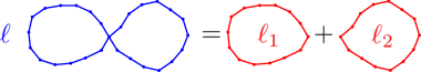
Figure 2. Decomposition of a figure-eight on a graph.

In our new setting, we shall also prove that the class $\mathcal{F}$ is stable by convolution. For two continuous functions $f_{1},f_{2}:\mathbb{R}_{>0}\rightarrow\mathbb{C}$, we define

$$f_{1}\ast f_{2}(\ell):=\int_{0}^{\ell}f_{1}(t)f_{2}(\ell-t)\,\mathrm{d}t=\int_{0}^{\ell}f_{1}(\ell-t)f_{2}(t)\,\mathrm{d}t.$$

Let us prove the following, which is a direct adaptation of the proof given by Friedman in the case of graphs [10, Theorem 7.2].

Proposition 3.5.

Let $f_{1},f_{2}\in\mathcal{F}$. Then, $f_{1}\ast f_{2}\in\mathcal{F}$.

Remark 3.6.

In the following, we will not use Proposition 3.5 exactly as such : unfortunately, in hyperbolic geometry, when we “concatenate” two closed geodesics by creating an intersection point, the length of the newly created closed geodesic is not the sum of the two original length (see Figure 10). This is a major difference between negative (but finite) curvature, and curvature $-\infty$ (i.e. the case of graphs). However, we believe the proof is quite enlightening in its simplicity – very similar techniques, yet more complex, are used in Section 7.

Proof.

Write $f_{i}(\ell)=p_{i}(\ell)\,e^{\ell}+r_{i}(\ell)$ with $|r_{i}(\ell)|\leq c_{i}(\ell+1)^{c_{i}}\,e^{\frac{\ell}{2}}$. We may assume that $c_{i}$ are integers. Then,

$$f_{1}\ast f_{2}=(p_{1}\exp)\ast(p_{2}\exp)+(p_{1}\exp)\ast r_{2}+(p_{2}\exp)\ast r_{1}+r_{1}\ast r_{2}.$$

First, we observe that

$$(p_{1}\exp)\ast(p_{2}\exp)(\ell)=\int_{0}^{\ell}p_{1}(t)\,e^{t}\,p_{2}(\ell-t)\,e^{\ell-t}\,\mathrm{d}t=P(\ell)\,e^{\ell}$$

where $P=p_{1}\ast p_{2}$ is a polynomial. Next, we have

$$|r_{1}\ast r_{2}(\ell)|\leq c_{1}c_{2}\,e^{\frac{\ell}{2}}\int_{0}^{\ell}(\ell-t+1)^{c_{1}}(t+1)^{c_{2}}\,\mathrm{d}t\leq c_{1}c_{2}e^{\frac{\ell}{2}}(\ell+1)^{c_{1}+c_{2}+1}.$$

Finally, we examine the crossed term $(p_{1}\exp)\ast r_{2}$.

$$(p_{1}\exp)\ast r_{2}(\ell) =e^{\ell}\int_{0}^{\ell}p_{1}(\ell-t)\,r_{2}(t)\,e^{-t}\,\mathrm{d}t$$

$$=e^{\ell}\int_{0}^{\infty}p_{1}(\ell-t)\,r_{2}(t)\,e^{-t}\,\mathrm{d}t-e^{\ell}\int_{\ell}^{\infty}p_{1}(\ell-t)\,r_{2}(t)\,e^{-t}\,\mathrm{d}t.$$

The function $\ell\mapsto\int_{0}^{\infty}p_{1}(\ell-t)\,r_{2}(t)\,e^{-t}\,\mathrm{d}t$ is a polynomial function. For the last term, it is bounded by

(3.6) $$\|p_{1}\|_{\ell^{\infty}}c_{2}\,e^{\ell}\int_{\ell}^{\infty}(t-\ell+1)^{\deg p_{1}}(t+1)^{c_{2}}e^{-\frac{t}{2}}\,\mathrm{d}t.$$

By an integration by parts, (3.6) is a function of the form $\ell\mapsto q(\ell)e^{\frac{\ell}{2}}$ with $q$ a polynomial, and in particular is bounded by $c^{\prime}(\ell+1)^{c^{\prime}}e^{\frac{\ell}{2}}$ for a constant $c^{\prime}>0$. The same argument of course applies to $(p_{2}\exp)\ast r_{1}$ and shows the announced result. ∎

3.4. Cancellations in the Selberg trace formula

We have seen in Section 3.2 that Friedman–Ramanujan functions arise naturally when computing expectations of sums over (simple) closed geodesics. The aim of this section is now to show how this information can be used, in particular in the study of the spectrum of the Laplacian.

The computations presented in this section are rather technical, and we invite the reader mostly interested in our new geometric techniques to skip it at first read. Indeed, while the ideas and results that we present below are a motivation for many results of Sections 4 to 8, they only come into play in Sections 9 and 10, when we actually study the spectral gap of random hyperbolic surfaces.

3.4.1. The Selberg trace formula

This beautiful formula, proven by Selberg in [39], relates the spectrum of the Laplacian on a hyperbolic surface to the lengths of all its closed geodesics. It reads, for a smooth even function $h:\mathbb{R}\rightarrow\mathbb{R}$,

(3.7) $$\sum_{j=0}^{+\infty}\hat{h}(r_{j}(X))=(g-1)\int_{\mathbb{R}}\hat{h}(r)\tanh(\pi r)r\,\mathrm{d}r+\sum_{\gamma\in\mathcal{P}(X)}\sum_{k=1}^{+\infty}\frac{\ell_{X}(\gamma)\,h(k\ell_{X}(\gamma))}{2\sinh\left(\frac{k\ell_{X}(\gamma)}{2}\right)}$$

where for all $j$, $r_{j}(X)\in\mathbb{R}\cup i[-\frac{1}{2},\frac{1}{2}]$ is a solution of $\lambda_{j}(X)=\frac{1}{4}+r_{j}(X)^{2}$, and the Fourier transform $\hat{h}$ is defined by $\hat{h}(r):=\int_{\mathbb{R}}h(\ell)\,e^{-ir\ell}\,\mathrm{d}\ell$. The formula is valid for a class of “nice” functions $h$; for our purposes, we will only consider functions $h$ of compact support, in which case the Selberg trace formula holds and both sums are absolutely convergent [3, Theorem 5.8].

Let us briefly describe the three terms of equation 3.7.

• The left hand side term is called the spectral side of the trace formula, and we will use this term to try and access information on the spectral gap $\lambda_{1}=\frac{1}{4}+r_{1}^{2}$.

• The first term on the right hand side is called the topological term, or integral term. The name “topological” refers to the fact that this term does not depend on the hyperbolic structure on the surface $X$, but only on its genus $g$. In particular, when studying random hyperbolic surfaces of genus $g$, this term is deterministic.

• The last term is the geometric term, in which appear every closed geodesic on the surface. We draw the attention to the fact that non-simple geodesics appear here, and there is a priori no known similar formula including only simple geodesics. Dealing with non-simple closed geodesics in the Selberg trace formula is one of the challenges we address in this article.

3.4.2. Spectral gap v.s. exponential growth

Due to the presence of a Fourier transform, and summations on the whole spectrum and all closed geodesics, the link made by the Selberg trace formula between geometry and spectrum is quite intricate, and using this formula requires a good choice of test function. A classic approach to access information on the spectral gap $\lambda_{1}$ using the Selberg trace formula, used in [45, 21] notably, is to observe that, if $\lambda_{1}=\frac{1}{4}+r_{1}^{2}<\frac{1}{4}$, then $r_{1}\in i\mathbb{R}$, and hence

$$\hat{h}(r_{1})=2\int_{0}^{+\infty}h(\ell)\cosh(\ell|r_{1}|)\,\mathrm{d}\ell.$$

The Fourier transform is therefore an integral against a growing exponential, at the rate $|r_{1}|=\sqrt{\frac{1}{4}-\lambda_{1}}$, rather than an oscillatory term.

We make the following choice of test function, similarly to [45, 21], that will allow us to exploit this exponential increase.

Notation 3.7.

Let $h:\mathbb{R}\rightarrow\mathbb{R}_{\geq 0}$ be a smooth even function, with compact support $[-1,1]$, such that $\hat{h}$ is non-negative on $\mathbb{R}\cup i[-\frac{1}{2},\frac{1}{2}]$. For any $L\geq 1$, let $h_{L}(\ell):=h(\frac{\ell}{L})$.

Remark 3.8.

Such a $h$ can be obtained by taking a square convolution $h:=H\ast H$ of a smooth function $H\geq 0$ supported on $[-\frac{1}{2},\frac{1}{2}]$, so that $\hat{h}=\hat{H}^{2}\geq 0$.

Remark 3.9.

The scaling parameter $L$ plays the role of a length-scale. Indeed, since the support of $h_{L}$ is $[-L,L]$, only geodesics of length $\leq L$ will contribute to the geometric term of the Selberg trace formula applied to $h_{L}$.

By analogy with graphs, we expect the natural length-scale we need to consider for the spectral gap problem to be $L=A\log(g)$, where $A\geq 1$ is a fixed constant. In [45, 21], the value $A=4$ is used to obtain the spectral gap $\frac{3}{16}-\epsilon$. We shall take $A=6$ to prove that $\lambda_{1}\geq\frac{2}{9}-\epsilon$, and see that arbitrarily large values of $A$ are required to reach $\frac{1}{4}-\epsilon$.

The following lemma allows us to relate the size of the spectral gap of a surface $X$ with the rate of exponential growth of the term $\hat{h}_{L}(r_{1}(X))$ of the Selberg trace formula.

Lemma 3.10.

Let $\alpha\in(0,\frac{1}{2})$. For any $0<\epsilon<\frac{1}{4}-\alpha^{2}$, there exists a constant $C_{\alpha,\epsilon}>0$ (depending on $h$) such that, for any hyperbolic surface $X$, any $L\geq 1$,

(3.8) $$\lambda_{1}(X)\leq\frac{1}{4}-\alpha^{2}-\epsilon\quad\Rightarrow\quad\hat{h}_{L}(r_{1}(X))\geq C_{\alpha,\epsilon}\,e^{(\alpha+\epsilon)L}.$$

Proof.

If $\lambda_{1}\leq\frac{1}{4}-\alpha^{2}-\epsilon<\frac{1}{4}$, then in particular $r_{1}\in i\mathbb{R}$. Then, by definition of $h_{L}$,

(3.9) $$\hat{h}_{L}(r_{1})=2L\int_{0}^{1}h(\ell)\,e^{|r_{1}|L\ell}\,\mathrm{d}\ell.$$

The hypothesis on $\lambda_{1}$ further implies that $|r_{1}|\geq\sqrt{\alpha^{2}+\epsilon}$. For $\alpha<1/2$, we have that $\frac{1}{4}-\alpha^{2}<1-2\alpha$, and hence $\epsilon<1-2\alpha$, which implies $\alpha+\epsilon<\sqrt{\alpha^{2}+\epsilon}$. Hence,

$$\hat{h}_{L}(r_{1})\geq 2\int_{\frac{\alpha+\epsilon}{\sqrt{\alpha^{2}+\epsilon}}}^{1}h(\ell)\,e^{\sqrt{\alpha^{2}+\epsilon}\,L\ell}\,\mathrm{d}\ell\geq C_{\alpha,\epsilon}\,e^{(\alpha+\epsilon)L}$$

since $h\geq 0$ by the hypothesis in 3.7. The implied constant can be taken to be $C_{\alpha,\epsilon}:=2\int_{(\alpha+\epsilon)/\sqrt{\alpha^{2}+\epsilon}}^{1}h(\ell)\,\mathrm{d}\ell$, which is positive because the support of the non-negative function $h$ is exactly $[-1,1]$. ∎

The following handy lemma clears up the Selberg trace formula, so that we can focus only on the terms which shall be crucial to our analysis.

Lemma 3.11.

Let $L\geq 1$, and $F:\mathbb{R}\rightarrow\mathbb{R}$ be a smooth even function, supported on $[-L,L]$, with $\hat{F}\geq 0$ on $\mathbb{R}\cup i[-\frac{1}{2},\frac{1}{2}]$. Then, for any $g\geq 2$,

$$\mathbb{E}_{g}^{\mathrm{\scriptsize{WP}}}\left[\hat{F}(r_{1}(X))\right]\leq\left\langle\ell\,F(\ell)\,e^{-\frac{\ell}{2}}\right\rangle_{g}^{{\mathrm{all}}}+C_{F}\,L^{2}g$$

for a constant $C_{F}:=c\lVert F\rVert_{\infty}+\lVert r\hat{F}(r)\rVert_{\infty}<+\infty$, where $c$ is a universal constant independent of $g$, $L$ and $F$.

Remark 3.12.

The constant $C_{F}$ is finite because $F$ is compactly supported, and hence $\hat{F}$ decays faster than any polynomial at infinity.

Remark 3.13.

The function $h_{L}$ defined in 3.7 clearly satisfies the hypotheses of the lemma. We have formulated the result in terms of a function $F$ with precise hypotheses because we shall later apply it to other test functions.

Lemmas 3.10 and 3.11 provide us with a strategy to prove probabilistic lower bounds on $\lambda_{1}$. First, we use 3.10 to write

$$\mathbb{P}_{g}^{\mathrm{\scriptsize{WP}}}\left(\lambda_{1}\leq\frac{1}{4}-\alpha^{2}-\epsilon\right)\leq\mathbb{P}_{g}^{\mathrm{\scriptsize{WP}}}\left(\hat{h}_{L}(r_{1})\geq C_{\alpha,\epsilon}\,e^{(\alpha+\epsilon)L}\right).$$

Using Markov’s inequality allows us to obtain that

$$\mathbb{P}_{g}^{\mathrm{\scriptsize{WP}}}\left(\lambda_{1}\leq\frac{1}{4}-\alpha^{2}-\epsilon\right)\leq\frac{\mathbb{E}_{g}^{\mathrm{\scriptsize{WP}}}\left[\hat{h}_{L}(r_{1})\right]}{C_{\alpha,\epsilon}\,e^{(\alpha+\epsilon)L}}.$$

We can then use 3.11 to obtain that, for $L:=A\log(g)$,

(3.10) $$\mathbb{P}_{g}^{\mathrm{\scriptsize{WP}}}\left(\lambda_{1}\leq\frac{1}{4}-\alpha^{2}-\epsilon\right)=\mathcal{O}_{\alpha,\epsilon,A}\left(\frac{\left\langle\ell h_{L}(\ell)\,e^{-\frac{\ell}{2}}\right\rangle_{g}^{{\mathrm{all}}}}{g^{(\alpha+\epsilon)A}}+(\log g)^{2}g^{1-(\alpha+\epsilon)A}\right),$$

since the constant $C_{h_{L}}$ can be bounded uniformly in $L$.

Let us pick a value of $A>1/(\alpha+\epsilon)$, such as $A:=1/\alpha$, so that $(\log g)^{2}g^{1-(\alpha+\epsilon)A}\rightarrow 0$. Equation 3.10 then reduces the spectral gap problem to proving that the geometric average $\langle\ell h_{L}(\ell)\,e^{-\frac{\ell}{2}}\rangle_{g}^{{\mathrm{all}}}$ is negligible compared to $e^{(\alpha+\epsilon)L}$.

As a conclusion, the trace method allows to bound $\mathbb{P}_{g}^{\mathrm{\scriptsize{WP}}}\left(\lambda_{1}\leq\frac{1}{4}-\alpha^{2}-\epsilon\right)$ in terms of the geometric average $\langle\ell h_{L}(\ell)\,e^{-\ell/2}\rangle_{g}^{{\mathrm{all}}}$ for $L=A\log(g)$. The parameter $\alpha$ needs to be small in order to obtain a spectral gap close to $1/4$. This naturally requires to look a length scale $L=A\log(g)$ with $A\geq 1/\alpha$, due to the presence of linear terms in the Selberg trace formula.

Proof of 3.11.

By the positivity hypothesis on $\hat{F}$, $\mathbb{E}_{g}^{\mathrm{\scriptsize{WP}}}[\hat{F}(r_{1})]$ is smaller than the expectation of the Selberg trace formula. Its integral term is independent of the surface, and smaller than $g\lVert r\hat{F}(r)\rVert_{\infty}$ because $\tanh\leq 1$. We hence are left with comparing

(3.11) $$\mathbb{E}_{g}^{\mathrm{\scriptsize{WP}}}\Bigg{[}\sum_{\gamma\in\mathcal{P}(X)}\sum_{k=1}^{+\infty}\frac{\ell_{X}(\gamma)\,F(k\ell_{X}(\gamma))}{2\sinh\left(\frac{k\ell_{X}(\gamma)}{2}\right)}\Bigg{]}$$

with the average $\langle\ell F(\ell)\,e^{-\frac{\ell}{2}}\rangle_{g}^{{\mathrm{all}}}$.

Let us first prove a bound on the sum over $k\geq 2$, i.e. the sum for non-primitive geodesics. Note that $x/\sinh\left(\frac{x}{2}\right)=\mathcal{O}\left((x+1)\,e^{-\frac{x}{2}}\right)$ for $x>0$. Hence, for any $0<\ell\leq L$,

$$\sum_{k=2}^{+\infty}\frac{\ell\,F(k\ell)}{2\sinh\left(\frac{k\ell}{2}\right)}=\mathcal{O}\left(L\|F\|_{\infty}\sum_{k=2}^{+\infty}e^{-\frac{k\ell}{2}}\right)=\mathcal{O}\left(L\|F\|_{\infty}\frac{e^{-\ell}}{\min(\ell,1)}\right)$$

because $\sum_{k=2}^{+\infty}e^{-k\ell/2}=e^{-\ell}/(1-e^{-\ell/2})$ and $1-e^{-\ell/2}\geq c\min(\ell,1)$ for a $c>0$.

We recall that $F$ is identically equal to zero outside $[-L,L]$. Hence, for a compact hyperbolic surface $X$ of genus $g$, we can apply the previous estimate to each $\ell=\ell_{X}(\gamma)$ appearing in the contribution of $X$ to the expectation (3.11) and deduce

(3.12) $$\sum_{\gamma\in\mathcal{P}(X)}\sum_{k=2}^{+\infty}\frac{\ell_{X}(\gamma)\,F(k\ell_{X}(\gamma))}{2\sinh\left(\frac{k\ell_{X}(\gamma)}{2}\right)}=\mathcal{O}\left(\frac{L\|F\|_{\infty}}{\min(\mathrm{sys}(X),1)}\sum_{\begin{subarray}{c}\gamma\in\mathcal{P}(X)\\ \ell_{X}(\gamma)\leq L\end{subarray}}e^{-\ell_{X}(\gamma)}\right)$$

where $\mathrm{sys}(X)$ is the length of the systole of $X$, its shortest closed geodesic. We bound uniformly in $X$ the sum above:

$$\sum_{\begin{subarray}{c}\gamma\in\mathcal{P}(X)\\ \ell_{X}(\gamma)\leq L\end{subarray}}e^{-\ell_{X}(\gamma)}\leq\sum_{j=0}^{\lceil L\rceil}e^{-j}\,\#\{\gamma\in\mathcal{P}(X)\,:\,j\leq\ell_{X}(\gamma)<j+1\}=\mathcal{O}\left(Lg\right)$$

by 2.1. As a consequence, taking the average of equation 3.12 yields

$$\mathbb{E}_{g}^{\mathrm{\scriptsize{WP}}}\Bigg{[}\sum_{\gamma\in\mathcal{P}(X)}\sum_{k=2}^{+\infty}\frac{\ell_{X}(\gamma)\,F(k\ell_{X}(\gamma))}{2\sinh\left(\frac{k\ell_{X}(\gamma)}{2}\right)}\Bigg{]}=\mathcal{O}\left(L^{2}g\|F\|_{\infty}\,\mathbb{E}_{g}^{\mathrm{\scriptsize{WP}}}\Bigg{[}\frac{1}{\min(\mathrm{sys}(X),1)}\Bigg{]}\right).$$

Mirzakhani proved in [27, Corollary 4.2] that the expectation above is finite and bounded uniformly in $g$, which is enough to conclude for this term.

All that is left to do to conclude is to substitute the $2\sinh\left(\frac{\ell}{2}\right)$ by the very close value $e^{\ell/2}$ in the term $k=1$ of equation 3.11. Because

$$\frac{1}{2\sinh\left(\frac{\ell}{2}\right)}-e^{-\frac{\ell}{2}}=\frac{1}{2\,e^{\ell}\,\sinh\left(\frac{\ell}{2}\right)}\leq\frac{e^{-\ell}}{\ell},$$

the error in doing so is bounded by

$$\|F\|_{\infty}\,\mathbb{E}_{g}^{\mathrm{\scriptsize{WP}}}\Bigg{[}\frac{1}{\min(\mathrm{sys}(X),1)}\sum_{\begin{subarray}{c}\gamma\in\mathcal{P}(X)\\ \ell_{X}(\gamma)\leq L\end{subarray}}e^{-\ell_{X}(\gamma)}\Bigg{]}$$

which we proved is bounded by a constant multiple of $gL\|F\|_{\infty}$. ∎

3.4.3. Necessity of expansions in powers of $1/g$

In [45, 21], Wu–Xue and Lipnowski–Wright obtained the spectral gap $3/16-\epsilon$ by using the method above. More precisely, the intermediate value $3/16$ arises because the average $\langle\ell h_{L}(\ell)\,e^{-\frac{\ell}{2}}\rangle_{g}^{{\mathrm{all}}}$ is estimated at the leading order as $g\rightarrow+\infty$, i.e. the computations are made up to errors with a $1/g$ decay. We now explain why, in order to reach the optimal spectral gap $1/4-\epsilon$, we need to go further and perform asymptotic expansions of averages $\langle F\rangle_{g}^{{\mathrm{all}}}$ in powers of $1/g$, which is one of the core objectives of this article.

Let us imagine that we are able to compute, exactly, any average $\langle F\rangle_{g}^{{\mathrm{all}}}$ up to error terms decaying as $1/g^{K}$ for a $K\geq 1$. This means that we will know the average $\langle\ell h_{L}(\ell)\,e^{-\frac{\ell}{2}}\rangle_{g}^{{\mathrm{all}}}$ up to errors of size roughly $e^{L/2}/g^{K}$, because the number of primitive closed geodesics shorter than $L$ behaves like $e^{L}/L$, by [18] (the factor $e^{L/2}$ comes from the presence of the exponential decay $e^{-\ell/2}$ in the average).

We recall that we saw in equation 3.10 that, for $\alpha>0$, in order to prove that $\mathbb{P}_{g}^{\mathrm{\scriptsize{WP}}}\left(\lambda_{1}\leq 1/4-\alpha^{2}-\epsilon\right)$ goes to $0$ as $g\rightarrow+\infty$, we need to prove that $\langle\ell h_{L}(\ell)\,e^{-\frac{\ell}{2}}\rangle_{g}^{{\mathrm{all}}}$ grows slower than $e^{\alpha L}$, for $L=A\log(g)$ and $A\geq 1/\alpha$. In particular, we will need the error term $\approx e^{L/2}/g^{K}$ produced when estimating this average to be smaller than $e^{\alpha L}$, which requires to assume that $A/2-K\leq\alpha A$. Hence, the hypotheses made so far on the parameters in the trace method can be listed as:

$$\frac{A}{2}-K\leq\alpha A\quad\text{and}\quad A\geq\frac{1}{\alpha}.$$

These conditions imply that $\alpha\geq 1/(2(K+1))$, which is a lower bound on the precision $\alpha$ that can be attained.

In other words, computing asymptotic expansions with remainders decaying like $1/g^{K}$ puts a natural limitation on the spectral gap $\lambda_{1}\geq 1/4-\alpha^{2}-\epsilon$ that can be obtained. These critical levels are summed up in Table 1; we see that the spectral gap $1/4-\epsilon$ requires expansions of arbitrary precision.

Order in expansion	Length scale $L$	Parameter $\alpha$	Hoped spectral gap
Leading (error $1/g$)	$4\log g$	$1/4$	$\lambda_{1}\geq\frac{3}{16}-\epsilon$
Second (error $1/g^{2}$)	$6\log g$	$1/6$	$\lambda_{1}\geq\frac{2}{9}-\epsilon$
…	…	…	…
Error $1/g^{K}$	$2(K+1)\log g$	$1/(2(K+1))$	$\lambda_{1}\geq\frac{1}{4}-\frac{1}{4(K+1)^{2}}-\epsilon$

Table 1. The spectral gap one can hope to obtain using the trace method, depending on the order of the asymptotic expansion in powers of $1/g$ at which we compute $\langle F\rangle_{g}^{{\mathrm{all}}}$.

The value $2/9-\epsilon$, obtained in this article, corresponds to understanding the second-order term, which is done here. We hope to generalise our methods in further articles, and ultimately reach the optimal spectral gap $1/4-\epsilon$.

3.4.4. The issue of the trivial eigenvalue

Unfortunately, the contribution of the trivial eigenvalue $\lambda_{0}=0$, for which $r_{0}=i/2$, will always be the dominant term in the Selberg trace formula. Indeed, $\hat{h}_{L}(i/2)$ grows almost like $e^{L/2}$ by equation 3.9. This is much bigger than the size $e^{\alpha L}$ we need to bound it with in order to prove that $\lambda_{1}\geq 1/4-\alpha^{2}-\epsilon$ with high probability. Actually, this rate of growth $e^{L/2}$ is exactly what we obtain by using Huber’s counting result [18] on the number of closed geodesics $\leq L$.

As a consequence, the method sketched in Section 3.4.2 will necessarily fail, if one does not find a mechanism to deal with the contribution of the trivial eigenvalue $\lambda_{0}=0$. The fact that the spectral gap only appears as a sub-dominant contribution in the trace method, which is hidden by a much bigger leading order, is always a challenge in spectral gap problems, see [10, 4] for instance in the case of graphs.

In [45, 21], when proving that $\lambda_{1}\geq 3/16-\epsilon$ typically, both teams rely on quite a miraculous phenomenon. They observe that the contribution of the trivial eigenvalue, $\hat{h}_{L}(i/2)$, and the average of the term corresponding to primitive simple geodesics in the Selberg trace formula are very close at the first order in $1/g$. Indeed, by using our first-order approximation for simple geodesics, 3.3, and the value of $f_{0}^{\mathrm{s}}$ from 3.4, we obtain that

$$\left\langle\frac{\ell\,h_{L}(\ell)}{2\sinh\left(\frac{\ell}{2}\right)}\right\rangle_{g}^{\mathrm{s}} =\int_{0}^{+\infty}\frac{\ell\,h_{L}(\ell)}{2\sinh\left(\frac{\ell}{2}\right)}\,\frac{4}{\ell}\sinh^{2}\left(\frac{\ell}{2}\right)\,\mathrm{d}\ell+\mathcal{O}\left(\frac{L^{c}e^{\frac{L}{2}}\|h_{L}\|_{\infty}}{g}\right)$$

$$=\underbrace{2\int_{0}^{+\infty}h_{L}(\ell)\cosh\left(\frac{\ell}{2}\right)\,\mathrm{d}\ell}_{\hat{h}_{L}(i/2)}+\mathcal{O}\left(\|h_{L}\|_{\infty}\left(1+\frac{L^{c}e^{\frac{L}{2}}}{g}\right)\right).$$

It is difficult to see how this approach could still function beyond the first-order estimate, and if it did, it would require tremendous effort and very accurate computation of all the coefficients appearing in the asymptotic expansion.

In this article, we suggest a fundamentally different approach to the one used in [45, 21], which we believe to be significantly more robust, and a good candidate to reach the optimal bound $\lambda_{1}\geq\frac{1}{4}-\epsilon$. The idea is to modify our test function to create a cancellation at the trivial eigenvalue $\lambda_{0}=0$. More precisely, we want to apply the Selberg trace formula to a function of Fourier transform $(\frac{1}{4}+r^{2})^{m}\hat{h}_{L}(r)$, which therefore has a zero of order $m$ at $r_{0}=i/2$. This is achieved by considering the new test function $\mathcal{D}^{m}h_{L}$, where $\mathcal{D}$ is the differential operator $\frac{1}{4}-\partial^{2}$. We prove the following reformulation of the spectral gap problem.

Lemma 3.14.

Let $h$ be a function satisfying the hypotheses of 3.7, and let us fix real numbers $\alpha\in(0,1/2)$ and $A\geq 1$. For any $\delta>0$, any $0<\epsilon<\frac{1}{4}-\alpha^{2}$, any integer $m\geq 1$, there exists a constant $C=C(h,\alpha,A,\epsilon,\delta,m)$ such that, for any large enough integer $g$ and for the length-scale $L=A\log g$,

$$\mathbb{P}_{g}^{\mathrm{\scriptsize{WP}}}\left(\delta\leq\lambda_{1}\leq\frac{1}{4}-\alpha^{2}-\epsilon\right)\leq\frac{C}{g^{(\alpha+\epsilon)A}}\left\langle\ell\,e^{-\frac{\ell}{2}}\,\mathcal{D}^{m}h_{L}(\ell)\right\rangle_{g}^{{\mathrm{all}}}+C\,\frac{g(\log g)^{2}}{g^{(\alpha+\epsilon)A}}\cdot$$

Remark 3.15.

The parameter $\delta$ is there because, if $\lambda_{1}$ is very small, then $\lambda_{1}^{m}\hat{h}_{L}(r_{1})$ will be small. However, this shall not matter, because we already know that $\mathbb{P}_{g}^{\mathrm{\scriptsize{WP}}}\left(\lambda_{1}\leq\delta\right)$ goes to $0$ as $g\rightarrow+\infty$ provided $\delta$ is small enough [27, 45, 21].

The hope is that, by cancelling the leading order $\hat{h}_{L}(i/2)$ on the spectral side of the Selberg trace formula, we have created enough cancellations for the average of the geometric term $\langle\ell e^{-\frac{\ell}{2}}\,\mathcal{D}^{m}h_{L}(\ell)\rangle_{g}^{{\mathrm{all}}}$ to be much smaller than it would be without the application of the differential operator $\mathcal{D}^{m}$. We shall provide methods to exhibit such cancellations in Section 3.4.5, which will further demonstrate the importance of Friedman–Ramanujan functions for the study of the spectral problem.

The proof is almost the same as the one sketched in Section 3.4.2, with a few small modifications. We provide the details here, because multiplication by the operator $\mathcal{D}^{m}$ makes us loose the fact that all terms in the Selberg trace formula are non-negative, which means we need to proceed with extra caution.

Proof.

By 3.10 applied to the function $h_{L}$, if $\delta\leq\lambda_{1}(X)\leq 1/4-\alpha^{2}-\epsilon$, then $\lambda_{1}(X)^{m}\hat{h}_{L}(r_{1}(X))\geq\delta^{m}C_{\alpha,\epsilon}\,e^{(\alpha+\epsilon)L}$ for a constant $C_{\alpha,\epsilon}>0$ (depending on $h$). As a consequence, by Markov’s inequality, using the non-negativity of $\lambda_{1}^{m}\hat{h}_{L}(r_{1})$,

$$\mathbb{P}_{g}^{\mathrm{\scriptsize{WP}}}\left(\delta\leq\lambda_{1}\leq\frac{1}{4}-\alpha^{2}-\epsilon\right)\leq\frac{1}{C_{\alpha,\epsilon}\delta^{m}g^{(\alpha+\epsilon)A}}\,\mathbb{E}_{g}^{\mathrm{\scriptsize{WP}}}\left[\lambda_{1}^{m}\hat{h}_{L}(r_{1})\right].$$

We then apply the Selberg trace formula to the function $\mathcal{D}^{m}h_{L}$, and more precisely the simplified version we have proven in 3.11. Note that the function $\mathcal{D}^{m}h_{L}$ satisfies the hypotheses of 3.11, because it is even, its support is included in the support of $h_{L}$, which is $[-L,L]$, and its Fourier transform is non-negative on $\mathbb{R}\cup i[-\frac{1}{2},\frac{1}{2}]$. Then,

$$\mathbb{P}_{g}^{\mathrm{\scriptsize{WP}}}\left(\delta\leq\lambda_{1}\leq\frac{1}{4}-\alpha^{2}-\epsilon\right)\leq\frac{C_{\alpha,\epsilon,\delta}}{g^{(\alpha+\epsilon)A}}\,\left(\langle\ell e^{-\frac{\ell}{2}}\,\mathcal{D}^{m}h_{L}(\ell)\rangle_{g}^{{\mathrm{all}}}+C_{\mathcal{D}^{m}h_{L}}L^{2}g\right)$$

and there is a universal constant $c$ such that

$$C_{\mathcal{D}^{m}h_{L}}\leq c\|\mathcal{D}^{m}h_{L}\|_{\infty}+\left\|r\,\left(\frac{1}{4}+r^{2}\right)^{m}\hat{h}_{L}(r)\right\|_{\infty}.$$

This quantity is bounded by a constant depending only on $m$ and $h$, because, for $L\geq 1$, the derivatives of $h_{L}(\ell):=h(\ell/L)$ are controlled by the derivatives of $h$, and because $\hat{h}_{L}(r)=L\hat{h}(rL)$, so the second norm is bounded by $\|r\left(1/4+r^{2}\right)^{m}\hat{h}\|_{\infty}$. ∎

3.4.5. Friedman–Ramanujan functions and cancellations

The reason for the introduction of Ramanujan functions in Friedman’s work [10] is that they are functions which exhibit some cancellations when computing averages of trace formulas. We shall extend this observation to hyperbolic surfaces: we show that Friedman–Ramanujan functions are functions which create non-trivial on-average cancellations in the Selberg trace formula.

Proposition 3.16.

Let $f$ be a Friedman–Ramanujan function in weak sense, and let $c_{f}$, $e_{f}$ denote its constant and exponent. Then, for any integer $m>\deg(f)$, there exists a constant $C_{m}$ such that for any $L\geq 1$,

(3.13) $$\left|\int_{0}^{L}f(\ell)\,e^{-\frac{\ell}{2}}\,\mathcal{D}^{m}h_{L}(\ell)\,\mathrm{d}\ell\right|\leq C_{m}(\lVert f\rVert_{\mathcal{F}_{w}}+c_{f}(L+1)^{e_{f}+1}).$$

Remark 3.17.

The constant $C_{m}$ depends on our fixed test function $h$. More precisely, it can be bounded by $C_{m}^{\prime}\max_{0\leq i\leq 2m}\|h^{(i)}\|_{\infty}$ for a constant $C_{m}^{\prime}$ depending only on $m$.

In other words, the integral in 3.16 has at-most polynomial growth in $L$, as opposed to the exponential growth one could expect, due to the fact that $f(\ell)\,e^{-\frac{\ell}{2}}$ is of size $\ell^{\deg f}\,e^{\ell/2}$ for large $\ell$. The definition of Friedman–Ramanujan function is made so that their principal term is always cancelled in integrals of the form (3.13). The reason for these cancellations is that functions of the form $p(\ell)\,e^{\ell/2}$ with $\deg(p)<m$ lie in the kernel of the operator $\mathcal{D}^{m}$.

Proof of 3.16.

We write $f(\ell)=p(\ell)\,e^{\ell}+r(\ell)$ for a polynomial function $p$ and a remainder satisfying

$$\int_{0}^{+\infty}\frac{|r(\ell)|}{(\ell+1)^{e_{f}}e^{\frac{\ell}{2}}}\,\mathrm{d}\ell\leq c_{f}.$$

Let us first estimate the integral of the remainder term:

$$\left|\int_{0}^{L}r(\ell)\,e^{-\frac{\ell}{2}}\,\mathcal{D}^{m}h_{L}(\ell)\,\mathrm{d}\ell\right|\leq\|\mathcal{D}^{m}h_{L}\|_{\infty}\int_{0}^{L}\frac{|r(\ell)|(L+1)^{e_{f}}}{(\ell+1)^{e_{f}}e^{\frac{\ell}{2}}}\,\mathrm{d}\ell=\mathcal{O}_{h,m}\left(c_{f}(L+1)^{e_{f}+1}\right)$$

because the derivatives of $h_{L}(\ell)=h(\ell/L)$ are bounded by that of $h$ for $L\geq 1$.

We are therefore left with the integral

$$\int_{0}^{L}p(\ell)\,e^{\frac{\ell}{2}}\,\mathcal{D}^{m}h_{L}(\ell)\,\mathrm{d}\ell.$$

We can estimate it using several integration by parts. Indeed, for any smooth functions $H_{1}$, $H_{2}$, if $\ell\mapsto H_{2}(\ell)$ is identically equal to zero for $\ell\geq L$, then

(3.14) $$\int_{0}^{L}H_{1}(\ell)\,\mathcal{D}H_{2}(\ell)\,\mathrm{d}\ell=\int_{0}^{L}\mathcal{D}H_{1}(\ell)\,H_{2}(\ell)\,\mathrm{d}\ell-H_{1}^{\prime}(0)H_{2}(0)+H_{1}(0)H_{2}^{\prime}(0)$$

because $H_{2}(L)=H_{2}^{\prime}(L)=0$. We apply this $m$ times to our integral, using the fact that $h_{L}$ and its derivatives vanish above $L$, and obtain that

(3.15) $$\int_{0}^{L}(p(\ell)\,e^{\frac{\ell}{2}})\,\mathcal{D}^{m}h_{L}(\ell)\,\mathrm{d}\ell=\int_{0}^{L}\mathcal{D}^{m}[p(\ell)e^{\frac{\ell}{2}}](\ell)\,h_{L}(\ell)\,\mathrm{d}\ell+\mathcal{O}_{h,m}\left(\|f\|_{\mathcal{F}_{w}}\right)$$

because the boundary terms appearing in (3.14) are linear combinations of products of the form $\partial^{i}h_{L}(0)\,\frac{\partial^{j}}{\partial\ell^{j}}[p(\ell)e^{\ell/2}](0)$ for $i,j\leq 2m$. The integral in the right hand side of equation 3.15 is equal to zero, because $\mathcal{D}^{m}[p(\ell)\,e^{\frac{\ell}{2}}]\equiv 0$ as soon as $m>\deg p$. ∎

In order to conclude this section with a strong motivation for the study of Friedman–Ramanujan functions in the context of the spectral gap question, we prove the following consequence of 3.16. This last statement uses some notations and results obtained in Sections 4 and 5, but will not be used until Sections 9 and 10.

Proposition 3.18.

Let $T$ be a local topological type. If Objective (FR) is true, i.e. for all $k\geq 0$, $\ell\mapsto\ell^{s_{T}}f_{k}^{T}(\ell)$ is Friedman–Ramanujan in the weak sense, then, for any integer $K\geq 1$, there exists constants $c_{K}^{T},m_{K}^{T}\geq 0$ such that for any large enough $g$, any $m\geq m_{K}^{T}$, any $\eta>0$ and $L\geq 1$,

$$\left\langle\ell\,e^{-\frac{\ell}{2}}\,\mathcal{D}^{m}h_{L}(\ell)\right\rangle_{g}^{{T}}=\mathcal{O}_{m,T,K,\eta}\left(L^{c_{K}^{T}}+\frac{e^{\frac{L}{2}+\eta L}}{g^{K}}\right).$$

This result is our motivation to prove Objective (FR) in all generality, which we expect to do in a follow-up paper. Indeed, recall that we presented in 3.14 a reformulation of the trace method, where we reduced the spectral gap problem to proving that the average $\langle\ell\,e^{-\frac{\ell}{2}}\,\mathcal{D}^{m}h_{L}(\ell)\rangle_{g}^{{\mathrm{all}}}$ is negligible compared to $g^{(\alpha+\epsilon)A}$, where $L=A\log g$, $A=2(K+1)=1/\alpha$, as explained in Table 1. Here, 3.18 tells us that, if Objective (FR) is true for a type $T$, then this objective is attained for the contribution of geodesics of type $T$ to the overall geometric average $\langle\ell\,e^{-\frac{\ell}{2}}\,\mathcal{D}^{m}h_{L}(\ell)\rangle_{g}^{{\mathrm{all}}}$.

For now, we have proved that Objective (FR) holds for the type “simple” in 3.3, and will extend it to any loop filling a pair of pants or once-holed torus in Sections 7 and 8. In particular, 3.18 is true in these cases.

Proof of 3.18.

Let $K\geq 1$. By 1.5,

$$\left\langle\ell\,e^{-\frac{\ell}{2}}\,\mathcal{D}^{m}h_{L}(\ell)\right\rangle_{g}^{{T}}=\int_{0}^{L}F^{T}_{g,K}(\ell)\,e^{-\frac{\ell}{2}}\,\mathcal{D}^{m}h_{L}(\ell)\,\mathrm{d}\ell+\mathcal{O}_{T,K,\eta}\left(\frac{\|e^{\frac{\ell}{2}+\eta\ell}\mathcal{D}^{m}h_{L}\|_{\infty}}{g^{K}}\right),$$

where $F_{g,K}^{T}(\ell):=\sum_{k=0}^{K-1}\ell f_{k}^{T}(\ell)/g^{k}$. By hypothesis, $\ell\mapsto F_{g,K}^{T}(\ell)$ is a Friedman–Ramanujan function in the weak sense, of degree at most $d_{K}^{T}:=\max_{0\leq k<K}\deg(\ell f_{k}^{T})$, of exponent at most $e_{K}^{T}:=\max_{0\leq k<K}e_{\ell f_{k}^{T}}$, of constant at most $\sum_{k=0}^{K-1}c_{\ell f_{k}^{T}}=\mathcal{O}_{T,K}\left(1\right)$, and of norm

$$\lVert F_{g,K}^{T}\rVert_{\mathcal{F}_{w}}\leq\sum_{k=0}^{K-1}\lVert\ell f_{k}^{T}(\ell)\rVert_{\mathcal{F}}=\mathcal{O}_{T,K}\left(1\right).$$

We take $m_{K}^{T}=d_{K}^{T}+1$ and $c_{K}^{T}:=e_{K}^{T}+1$, and apply 3.16 to conclude. ∎

4. Local topological types of closed loops

One of the aims of this article is to generalise methods to compute averages for simple geodesics to more elaborate topologies. In order to do so, we need to introduce a few notations and concepts related to non-simple closed geodesics on a surface.

4.1. Surface filled by a loop

A challenge faced when studying general loops is that the machinery developed by Mirzakhani in [26, 27] only applies to multi-curves, i.e. families of simple disjoint loops. A way around this difficulty, already used in [28, 45, 21], is to associate to any loop a surface that it fills, using the following procedure.

Definition 4.1.

Let $X$ be a compact hyperbolic surface, and $\gamma$ be a loop on $X$. We assume that $\gamma$ is in minimal position, i.e. that it minimises the number of self-intersections in its free-homotopy class. We define the surface $S(\gamma)$ filled by $\gamma$ the following way.

1. We take a regular neighbourhood of $\gamma$ in $X$, $\mathcal{V}_{\epsilon}(\gamma):=\{x\in X\,:\,\operatorname{dist}(x,\gamma)<\epsilon\}$ for $\epsilon>0$ small enough so that $\mathcal{V}_{\epsilon}(\gamma)$ retracts to $\gamma$.

2. The bordered surface $X\setminus\mathcal{V}_{\epsilon}(\gamma)$ has $q_{0}\geq 1$ connected components $C_{1}\sqcup\ldots\sqcup C_{q_{0}}$. We take

   $$S(\gamma):=\mathcal{V}_{\epsilon}(\gamma)\cup\bigcup_{i:C_{i}\text{ is a disk}}C_{i},$$

   i.e. we add every disk to $\mathcal{V}_{\epsilon}(\gamma)$, to form $S(\gamma)$.

The surface $S(\gamma)$ is a subsurface of $X$, possibly with a boundary, filled by $\gamma$. It does not depend on the choice of $\epsilon>0$, in the sense that the filled surfaces obtained using two small values of $\epsilon$ are isotopic. Similarly, the metric on $X$ is solely used to define the regular neighbourhood, and replacing it by another metric yields the same filled surface, up to isotopy. The notion of filled surface only depends on the topology of the loop $\gamma$ within the topological surface $X$.

The boundary of $S(\gamma)$ is a family of simple loops, which we orient so that $S(\gamma)$ lies on the left side of each boundary components. The motivation for introducing $S(\gamma)$ is that the boundary the surface filled by $\gamma$ is (almost) a multi-curve, and can hence be dealt with using Mirzakhani’s tools (almost because pairs of these boundary loops might satisfy $\gamma_{1}\,\raisebox{-2.84526pt}{$\mathrel{\ensurestackMath{\stackengine{-.2pt}{\scriptscriptstyle\mathrm{h}}{\sim}{O}{c}{F}{F}{S}}}$}\,\gamma_{2}^{-1}$ whenever there is a cylinder in $X\setminus S(\gamma)$).

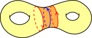
(a) A simple curve.

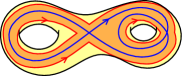
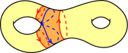
(b) Two non-simple curves filling a pair of pants.

Figure 3. Examples of filled surfaces.

Example 4.2.

The surface filled by a simple essential loop is a cylinder. If $\gamma$ is a loop with exactly one self-intersection, then $S(\gamma)$ is a pair of pants.

Three examples of loops and their filled surfaces are represented in Figure 3. Note that, in the first example of Figure 3(b), we added a disk to the regular neighbourhood to form the filled surface. In the last picture, we replaced the filled surface by another isotopic surface, for the sake of readability.

We prove the following, using a classic result of Graaf–Schrijver [13].

Lemma 4.3.

Let $X$ be a compact hyperbolic surface. If $\gamma$ and $\gamma^{\prime}$ are two closed loops in minimal position in $X$ in the same free-homotopy class, then there exists an isotopy of $X$ sending $S(\gamma)$ on $S(\gamma^{\prime})$ and $\gamma$ on a closed loop freely homotopic to $\gamma^{\prime}$ in $S(\gamma^{\prime})$.

As a consequence, the surface $S(\gamma)$ filled by $\gamma$ is well-defined (up to isotopy) for a free-homotopy class $\gamma\in\mathcal{P}(X)$. We shall see in the proof that this is true thanks to the fact that we added all disks to the regular neighbourhood of $\gamma$.

Proof.

First, we observe that if $\gamma$ and $\gamma^{\prime}$ are isotopic, that is to say if there exists an isotopy $\phi_{t}:X\rightarrow X$, $0\leq t\leq 1$, such that $\phi_{1}\circ\gamma=\gamma^{\prime}$, then the claim is trivially satisfied. Indeed, in this case, for small enough $\epsilon>0$, we can modify the isotopy $(\phi_{t})_{t}$ to obtain a new isotopy $(\psi_{t})_{t}$ which coincides with $(\phi_{t})_{t}$ on all points of $\gamma$ and sends the regular neighbourhood $\mathcal{V}_{\epsilon}(\gamma)$ onto the regular neighbourhood $\mathcal{V}_{\epsilon}(\gamma^{\prime})$ of $\gamma^{\prime}$. Then, the isotopy $\psi_{1}$ is an homeomorphism from each connected components of $X\setminus\mathcal{V}_{\epsilon}(\gamma)$ to each component of $X\setminus\mathcal{V}_{\epsilon}(\gamma^{\prime})$, and in particular sends contractible components to contractible components. Hence, the isotopy $(\psi_{t})_{t}$ sends $S(\gamma)$ on $S(\gamma^{\prime})$ and $\gamma$ on $\gamma^{\prime}$, and our claim is satisfied.

More generally, by [13], because $\gamma$ and $\gamma^{\prime}$ are freely homotopic and both in minimal position, there is a finite sequence of third Reidemeister moves that send $\gamma$ to a loop $\tilde{\gamma}$ isotopic to $\gamma^{\prime}$. As a consequence, we simply need to prove our claim for two loops $\gamma$, $\gamma^{\prime}$ differing by a third Reidemeister move, as represented in Figure 4.

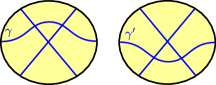
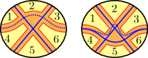
Figure 4. On the left hand side, a portion of two loops $\gamma$, $\gamma^{\prime}$ differing only by a third Reidemeister move. On the right hand side, in orange, their respective regular neighbourhood, to which we added the central disk. We labelled the (possibly non-distinct) connected components of the complement of this region to highlight their correspondence.

We observe on Figure 4 that, thanks to the addition of the central contractible component in the construction of $S(\gamma)$ and $S(\gamma^{\prime})$, there exists an isotopy $(\phi_{t})_{0\leq t\leq 1}$ (identically equal to the identity outside the neighbourhood where the Reidemeister move occurs) sending $S(\gamma)$ to $S(\gamma^{\prime})$. The image of $\gamma$ by such an isotopy is represented by the dotted line in the last part of Figure 4, and it is clear that $\phi_{1}\circ\gamma$ and $\gamma^{\prime}$ are freely homotopic within $S(\gamma^{\prime})$. ∎

The following observation on the boundary length of $S(\gamma)$ will be useful.

Lemma 4.4.

Let $X$ be a compact hyperbolic surface, and $\gamma\in\mathcal{P}(X)$. Let $\hat{S}(\gamma)$ denote the surface isotopic to $S(\gamma)$ in $X$ with geodesic boundary. Then, $\ell_{X}(\partial\hat{S}(\gamma))\leq 2\ell_{X}(\gamma)$.

Proof.

For any $\eta>0$, we can pick the $\epsilon$ for defining the regular neighbourhood of $\gamma$ such that the length of its boundary is $\leq 2\ell_{X}(\gamma)+\eta$. Then, the length of the boundary only diminishes when adding disks to the complement, and when replacing every component of the boundary by a geodesic representative, so $\ell_{X}(\partial\hat{S}(\gamma))\leq 2\ell_{X}(\gamma)+\eta$. We obtain the result by letting $\eta\rightarrow 0$. ∎

4.2. Definition of local topological type

Let us define a notion of local (topological) type. Examples of local types are presented in Figure 5, the type “simple” being the leftmost one.

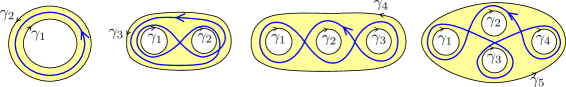
Figure 5. Examples of local topological types.

Notation 4.5.

To any pair of integers $(g_{S},n_{S})$ such that $-\chi_{S}:=2g_{S}-2+n_{S}\geq 0$, we shall associate a fixed smooth oriented surface $S$ of signature $(g_{S},n_{S})$. We further fix a numbering of the $n_{S}$ boundary components of $S$, and denote for each $1\leq i\leq n_{S}$ as $\gamma_{i}$ the $i$-th boundary loop of $S$, oriented so that $S$ lies on the left hand side of $\gamma_{i}$. The data of the pair of integers $(g_{S},n_{S})$, or equivalently of the surface $S$, is called a filling type.

Definition 4.6.

A local loop is a pair $(S,\gamma)$, where $S$ is a filling type and $\gamma$ is a primitive loop filling $S$. Two local loops $(S,\gamma)$ and $(S^{\prime},\gamma^{\prime})$ are said to be locally equivalent if $S=S^{\prime}$ (i.e. $g_{S}=g_{S^{\prime}}$ and $n_{S}=n_{S^{\prime}}$), and there exists a positive homeomorphism $\psi:S\rightarrow S$, possibly permuting the boundary components of $S$, such that $\psi\circ\gamma$ is freely homotopic to $\gamma^{\prime}$. This defines an equivalence relation  $\mathrel{\ensurestackMath{\stackengine{-.2pt}{\scriptscriptstyle\mathrm{loc}}{\sim}{O}{c}{F}{F}{S}}}$  on local loops. Equivalence classes for this relation are denoted as $[S,\gamma]_{\mathrm{loc}}$ and called local (topological) types of loops.

Example 4.7.

Figure 6. Two representatives of the local type “simple”.

There is exactly one local topological type filling a cylinder (i.e. of filling type $(0,2)$), which we shall refer to as the local type “simple”. Indeed, there are exactly two homotopy classes of primitive loops filling a cylinder, represented in Figure 6. Taking a positive homeomorphism permuting the two boundary components of the cylinder allows to observe that these two local loops are equivalent.

Example 4.8.

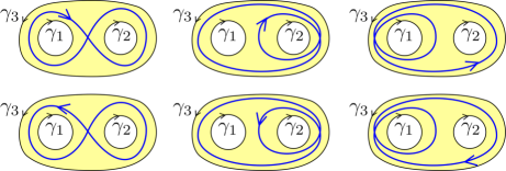
Figure 7. Six representatives of the local type “eight”.

We call “figure-eight” the local type of which six representatives are depicted in Figure 7. The figure-eight is of filling type $(0,3)$, i.e. it fills a pair of pants. As in the previous example, these different representatives can be shown to be equivalent by applying a positive homeomorphism of the pair of pants permuting its boundary components. More precisely, the six representatives correspond to the six permutations of the set $\{1,2,3\}$; in reading order, $\operatorname{id}$, $(123)$, $(132)$, $(12)$, $(13)$, $(23)$.

4.3. Local topological type of a loop on a surface of genus $g$

Let us now define a notion of local topological type for loops on a compact hyperbolic surface of genus $g$, for $g\geq 2$. We shall do this for loops on the base surface $S_{g}$, which we endow with a fixed hyperbolic metric for the purpose of defining regular neighbourhoods.

Definition 4.9.

Let $[S,\gamma]_{\mathrm{loc}}$ be a local topological type. A loop $\gamma_{g}$ on the base surface $S_{g}$ is said to belong to the local topological type $[S,\gamma]_{\mathrm{loc}}$ if there exists a positive homeomorphism $\phi:S(\gamma_{g})\rightarrow S$ such that the loops $\phi\circ\gamma_{g}$ and $\gamma$ are freely homotopic in $S$. In that case, we write $\gamma_{g}\in[S,\gamma]_{\mathrm{loc}}^{g}$. We say that two loops $\gamma_{g}$, $\gamma_{g}^{\prime}$ on $S_{g}$ are locally equivalent, and write $\gamma_{g}\,\raisebox{-2.84526pt}{$\mathrel{\ensurestackMath{\stackengine{-.2pt}{\scriptscriptstyle\mathrm{loc}}{\sim}{O}{c}{F}{F}{S}}}$}\,\gamma_{g}^{\prime}$, if $\gamma_{g}$ and $\gamma_{g}^{\prime}$ belong to the same local topological type.

It is clear that the definition does not depend on the choice of the representative $(S,\gamma)$ in the local topological type. The fact that it does not depend on the choice of representative in the free-homotopy classes $\gamma_{g}$ and $\gamma_{g}^{\prime}$ either is a consequence of 4.3.

Example 4.10.

The loops on the base surface $S_{g}$ belonging to the local type “simple” are exactly all simple loops on $S_{g}$. Indeed, take $\gamma_{g}\in\mathcal{P}_{g}$.

• If $\gamma_{g}$ is simple, then its regular neighbourhood is a cylinder. Because $\gamma_{g}$ is not contractible, $S(\gamma_{g})$ is exactly this cylinder, and then $\gamma_{g}$ is its core. It directly follows that $\gamma_{g}$ belong to the local type “simple”.

• If $\gamma_{g}$ belongs to the local type “simple”, then $S(\gamma_{g})$ is a topological cylinder, and $\gamma_{g}$ is homotopic to its core. As a consequence, the homotopy class $\gamma_{g}$ admits a simple representative, which means that $\gamma_{g}$ is simple.

4.4. Comparison with mapping-class-group equivalence

4.10 shows that the notion of local equivalence and $\mathrm{MCG}_{g}$-equivalence do not coincide. Indeed, there are several distinct orbits of simple loops for $\mathrm{MCG}_{g}$: non-separating loops, and loops separating two surfaces on their left and right side, of respective signatures $(i,1)$ and $(g-i,1)$ for a $1\leq i\leq g-1$. This is a general fact: equivalence classes for $\mathrm{MCG}_{g}$ are included in equivalence classes for  $\mathrel{\ensurestackMath{\stackengine{-.2pt}{\scriptscriptstyle\mathrm{loc}}{\sim}{O}{c}{F}{F}{S}}}$ , as shown in the following lemma.

Lemma 4.11.

Let $\gamma_{g}$, $\gamma_{g}^{\prime}\in\mathcal{P}_{g}$. If $\gamma_{g}\,\raisebox{-2.84526pt}{$\mathrel{\ensurestackMath{\stackengine{-.2pt}{\scriptscriptstyle\mathrm{MCG}}{\sim}{O}{c}{F}{F}{S}}}$}\,\gamma_{g}^{\prime}$, then $\gamma_{g}\,\raisebox{-2.84526pt}{$\mathrel{\ensurestackMath{\stackengine{-.2pt}{\scriptscriptstyle\mathrm{loc}}{\sim}{O}{c}{F}{F}{S}}}$}\,\gamma_{g}^{\prime}$.

Proof.

We assume that there exists a homeomorphism $\phi:S_{g}\rightarrow S_{g}$ sending $\gamma_{g}$ on $\gamma_{g}^{\prime}$. Then, by definition of the filled surface associated to a loop, the image of $S(\gamma_{g})$ by $\phi$ is isotopic to $S(\gamma_{g}^{\prime})$. As a consequence, by composition, there exists a homeomorphism $\psi:S_{g}\rightarrow S_{g}$ sending $S(\gamma_{g})$ on $S(\gamma_{g}^{\prime})$ and $\gamma_{g}$ on $\gamma_{g}^{\prime}$, which implies our claim. ∎

The choice of the name “local equivalence” comes from the fact that this notion only encaptures the topology of the filled surface $S(\gamma_{g})$ and of the loop $\gamma_{g}$ within it, but does no say anything about the topology of the complement $S_{g}\setminus S(\gamma_{g})$. To the contrary, if two loops $\gamma_{g},\gamma_{g}^{\prime}$ are in the same $\mathrm{MCG}_{g}$-orbit, then the topologies of $S_{g}\setminus S(\gamma_{g})$ and $S_{g}\setminus S(\gamma_{g}^{\prime})$ need to be “the same”, in a way which will be made more precise in the following section.

4.5. Realisations of a filling type

In order to describe more precisely the way that a local equivalence class $[S,\gamma]_{\mathrm{loc}}^{g}$ is partitioned in $\mathrm{MCG}_{g}$-orbits, we introduce the following notion.

Definition 4.12.

Let $S$ be a filling type, and $g\geq 2$. We call realisation of $S$ in $S_{g}$ any pair $R=(\vec{I},\vec{g})$, where:

• $\vec{I}$ is a partition of $\partial S=\{1,\ldots,n_{S}\}$ into $q\geq 1$ non-empty sets $I_{1},\ldots,I_{q}$, numbered such that $j\mapsto\min I_{j}$ is an increasing function;

• $\vec{g}=(g_{1},\ldots,g_{q})$ is a vector of non-negative integers;

• for any $1\leq j\leq q$, $\chi_{j}:=2-2g_{j}-n_{j}\leq 0$, where $n_{j}:=\#I_{j}$;

• for $\chi_{g}:=\chi(S_{g})=2-2g$ and $\chi_{S}:=2-2g_{S}-n_{S}$, we have

  (4.1) $$\chi_{S}+\sum_{j=1}^{q}\chi_{j}=\chi_{g}.$$

The set of realisations of $S$ in $S_{g}$ is denoted as $R_{g}(S)$.

Remark 4.13.

We observe that, since $\vec{I}$ is a partition of $\partial S$, we have that $\sum_{j=1}^{q}n_{j}=n_{S}$, and we can therefore rewrite equation 4.1 as

(4.2) $$\sum_{j=1}^{q}g_{j}+g_{S}+n_{S}-q=g.$$

Notation 4.14.

Let $S$ be a filling type, $g\geq 2$, and $R=(\vec{I},\vec{g})\in R_{g}(S)$. We can construct a compact surface $S_{g}(S,R)$ by gluing, for all $1\leq j\leq q$, a surface of signature $(g_{j},n_{j})$ on the boundary components of $S$ belonging in $I_{j}$. By equation 4.1, the resulting surface is a compact surface of genus $g$, and hence there exists a positive homeomorphism $\phi_{g,S,R}$ from $S_{g}(S,R)$ to $S_{g}$.

Remark 4.15.

Note that, if $(g_{j},n_{j})=(0,2)$, then the surface we glue is a cylinder, which corresponds to gluing two boundary components of $S$ together. In all other cases, we glue an honest surface of negative Euler characteristic to $\partial S$.

Notation 4.16.

For any local type $T=[S,\gamma]_{\mathrm{loc}}$, we fix a choice of representative $(S,\gamma^{T})$, meaning that $\gamma^{T}$ is a fixed loop on the topological surface $S$, in the local equivalence class $T$. Then, for any $g\geq 2$ and any realisation $R\in R_{g}(S)$, we denote as $\mathrm{Orb}_{g}^{T}(R)$ the orbit of $\phi_{g,S,R}(\gamma^{T})$ for the action of $\mathrm{MCG}_{g}$.

We furthermore denote as $\Gamma_{g}^{S}(R)$ the multi-curve $\phi_{g,S,R}(\partial S)$ on $S_{g}$, with the numbering and orientation of $\partial S$, and the following convention. For any index $j\in\{1,\ldots,q\}$ such that $I_{j}=\{i,i^{\prime}\}$ with $i<i^{\prime}$ and $g_{j}=2$ (if such an index exists), then we do not include the $i^{\prime}$-th component of $\partial S$ in $\Gamma_{g}^{S}(R)$. We do this so that all components of $\Gamma_{g}^{S}(R)$ are distinct, because when $(g_{j},n_{j})=(0,2)$, we glue a cylinder to $\partial S$, so its $i$-th and $i^{\prime}$-th boundary components become homotopic.

Remark 4.17.

The orbit $\mathrm{Orb}_{g}^{T}(R)$ does not depend on the choice of the homeomorphism $\phi_{g,S,R}$. However, it does a priori depend on the choice of the representative $\gamma$ of the local type, which is why we fixed such a representative.

It is clear with these notations that, for any loop $\gamma_{g}\in T^{g}$, there exists a realisation $R$ of $S$ in $S_{g}$ such that $\gamma_{g}\in\mathrm{Orb}_{g}^{T}(R)$. So, realisations do enumerate all possible embeddings of a local type in a surface of genus $g$. The following immediate lemma allows to count the number of appearances of each $\mathrm{MCG}_{g}$-orbit whilst listing all realisations $R$.

Lemma 4.18.

Let $T$ be a local type of filling type $S$, and $g\geq 2$. If $R=(\vec{I},\vec{g})$ and $R^{\prime}=(\vec{I}^{\prime},\vec{g}^{\prime})$ are two realisations of $S$ in $S_{g}$, we have that $\mathrm{Orb}_{g}^{T}(R)=\mathrm{Orb}_{g}^{T}(R^{\prime})$ if and only if the following conditions are satisfied:

• there exists a positive homeomorphism $\phi:S\rightarrow S$, possibly permuting the boundary components of $S$, such that $\phi(\gamma^{T})$ and $\gamma^{T}$ are freely homotopic in $S$;

• for all $1\leq j\leq q$, $\phi$ sends the components of $\partial S$ lying in $I_{j}$ on the components lying in $I_{j^{\prime}}^{\prime}$ for a $1\leq j^{\prime}\leq q$ such that $g_{j}=g_{j^{\prime}}^{\prime}$.

We notice that, whenever $\phi$ acts trivially on $\partial S$, these conditions imply that $R=R^{\prime}$ thanks to our numbering convention for $\vec{I}$. As a consequence, several realisations can get associated to the same orbit, but only in the case where the loop $\gamma^{T}$ has non-trivial symmetries in $S$. This motivates the following definition.

Definition 4.19.

Let $T$ be a local topological type of filling type $S$. We call multiplicity of $T$ the cardinal $m(T)$ of the subgroup of permutations of $\partial S=\{1,\ldots,n_{S}\}$ induced by positive homeomorphisms $\phi:S\rightarrow S$ such that $\gamma^{T}$ and $\phi(\gamma^{T})$ are homotopic.

Note that, while the subgroup in 4.19 depends on the choice of the representative $\gamma^{T}$, its cardinality does not, so the multiplicity of a local type is well-defined.

Example 4.20.

The image of the figure-eight by all permutations of $\{1,2,3\}$ is represented in Figure 7; we see that, in this case, $m(T)=1$. However, in the third example of Figure 5, the multiplicity is $2$ because the permutation $(13)$ stabilises the loop $\gamma$.

5. Average over a local type

The aim of this section is to define the average $\langle F\rangle_{g}^{{T}}$ of a test function over a local type $T$, and to provide a method to express and estimate it. In particular, we shall:

• provide a formula for $\langle F\rangle_{g}^{{T}}$ in terms of Weil–Petersson volumes in 5.5;

• prove it can be written as a density in 5.9;

• expand it in powers of $1/g$ in 5.14.

5.1. Definition

Let us define the average $\langle F\rangle_{g}^{{T}}$ of a test function $F$ over a local topological type $T$.

Definition 5.1.

We call admissible test function any measurable function $F:\mathbb{R}_{\geq 0}\rightarrow\mathbb{C}$ that is either compactly supported, or non-negative.

Remark 5.2.

Actually, the results in this paper hold for a more general class of test functions, we only need to assume that they decay sufficiently fast at infinity so that all quantities mentioned converge.

The invariance of local types by action of the mapping-class group allows us to make the following definition.

Definition 5.3.

Let $T$ be a local topological type. For any admissible test function $F$, any $g\geq 2$, we define the $T$-average of $F$ over surfaces of genus $g$ to be

(5.1) $$\langle F\rangle_{g}^{{T}}:=\mathbb{E}_{g}^{\mathrm{\scriptsize{WP}}}\Bigg{[}\sum_{\gamma_{g}\in T^{g}}F(\ell_{X}(\gamma_{g}))\Bigg{]}.$$

We notice that this coincides with the definition of $\langle F\rangle_{g}^{{\mathrm{s}}}$ for the local type “simple”. Obviously, we have that

$$\langle F\rangle_{g}^{{\mathrm{all}}}=\sum_{T\text{ local type}}\langle F\rangle_{g}^{{T}}.$$

Remark 5.4.

An interesting benefit from splitting the average $\langle F\rangle_{g}^{{\mathrm{all}}}$ by local topological type rather than $\mathrm{MCG}_{g}$-orbit is that the set of local types is fixed and independent of the genus $g$, whilst the number of $\mathrm{MCG}_{g}$-orbits of loops grows as a function of $g$.

5.2. Integration formula for averages over a local type

We are now ready to write an integration formula for the average $\langle F\rangle_{g}^{{T}}$, for any local type $T$.

Theorem 5.5.

Let $T$ be a local topological type of filling type $S$. Then, for any $g\geq 3$, any admissible test function $F$,

(5.2) $$\langle F\rangle_{g}^{{T}}=\frac{1}{m(T)}\int_{\mathbb{R}_{>0}^{n_{S}}}\mathbb{E}_{S}[F^{T}\,|\,\ell(\partial S)=\mathbf{x}]\,\phi_{g}^{S}(\mathbf{x})\,\mathrm{d}\mathbf{x}$$

where

(5.3) $$\mathbb{E}_{S}[F^{T}\,|\,\ell(\partial S)=\mathbf{x}]:=\frac{1}{V_{g_{S},n_{S}}(\mathbf{x})}\int_{\mathcal{M}_{g_{S},n_{S}}(\mathbf{x})}\sum_{\alpha\in\mathrm{Orb}_{S}(\gamma^{T})}F(\ell_{Y}(\alpha))\,\mathrm{d}\mathrm{Vol}_{g_{S},n_{S},\mathbf{x}}^{\mathrm{\scriptsize{WP}}}(Y)$$

with $\mathrm{Orb}_{S}(\gamma^{T})$ the orbit of $\gamma^{T}$ for the action of the mapping-class group of $S$ (fixing the boundary components of $S$), and

(5.4) $$\phi_{g}^{S}(\mathbf{x}):=x_{1}\ldots x_{n_{S}}\frac{V_{g_{S},n_{S}}(\mathbf{x})}{V_{g}}\sum_{R\in R_{g}(S)}\prod_{j=1}^{q}V_{g_{j},n_{j}}(\mathbf{x}^{(j)}),$$

with the convention that $V_{0,2}(x,y):=\frac{1}{x}\,\delta(x-y)$ where $\delta$ is the Dirac delta distribution, and $\mathbf{x}^{(j)}=(x_{i},i\in I_{j})\in\mathbb{R}^{n_{j}}$.

Example 5.6.

The multiplicity of the type “simple” is $1$, and the definition of $\phi_{g}^{(0,2)}(x,y)$ contains a $\delta(x-y)$, so we shall only compute it on the diagonal $x=y$. We have

(5.5) $$\phi_{g}^{(0,2)}(x,x)=\frac{x}{V_{g}}\left(V_{g-1,2}(x,x)+\sum_{i=1}^{g-1}V_{i,1}(x)V_{g-i,1}(x)\right).$$

Furthermore, the conditional expectation defined in equation 5.3 is equal to $F(x)$, because the length of a simple loop and the boundary geodesics of the cylinder it fills coincide. We therefore recover the expression for $\langle F\rangle_{g}^{{\mathrm{s}}}$ that was obtained in Section 3.2.

Example 5.7.

Let $\gamma$ be a loop filling the pair of pants $P$ (i.e. our fixed surface of signature $(0,3)$). Then, the length of $\gamma$ is an analytic function of the lengths of the three boundary components $(x_{1},x_{2},x_{3})$ of $P$, which we shall denote as $\mathcal{L}_{\gamma}:\mathbb{R}_{>0}^{3}\rightarrow\mathbb{R}_{>0}$. We then have that

$$\langle F\rangle_{g}^{{[P,\gamma]_{\mathrm{loc}}}}=\frac{1}{m(\gamma)}\iiint_{\mathbb{R}_{>0}^{3}}F(\mathcal{L}_{\gamma}(x_{1},x_{2},x_{3}))\,\phi_{g}^{P}(x_{1},x_{2},x_{3})\,\mathrm{d}x_{1}\,\mathrm{d}x_{2}\,\mathrm{d}x_{3}$$

where $m(\gamma)\in\{1,2,3,6\}$ is the number of permutations of $\{1,2,3\}$ stabilising the homotopy class of $\gamma$, and

$$\phi_{g}^{P}(\mathbf{x})=\frac{x_{1}x_{2}x_{3}}{V_{g}}\left[V_{g-2,3}(x_{1},x_{2},x_{3})+\sum_{g_{1}+g_{2}+g_{3}=g}V_{g_{1},1}(x_{1})V_{g_{2},1}(x_{2})V_{g_{3},1}(x_{3})\right.\\ \left.+\sum_{\begin{subarray}{c}\{i_{1},i_{2},i_{3}\}\\ =\{1,2,3\}\end{subarray}}\left(\frac{\delta(x_{i_{1}}-x_{i_{2}})}{x_{i_{1}}}V_{g-1,1}(x_{i_{3}})+\sum_{i=1}^{g-2}V_{i,2}(x_{i_{1}},x_{i_{2}})V_{g-i-1,1}(x_{i_{3}})\right)\right].$$

Remark 5.8.

In the two previous examples, the conditional expectation (5.3) has a very simple expression because the length of the loop $\gamma$ is entirely determined by the lengths of the boundary components of the surface it fills. However, in all cases but these ones, the moduli space of the filled surface is a space of $>0$ dimension on which an average takes place, and the sum over the mapping-class group is not reduced to an element. Understanding the behaviour of the function $\mathbf{x}\mapsto\mathbb{E}_{S}[F^{T}\,|\,\ell(\partial S)=\mathbf{x}]$, for a general local type $T$, is a significant challenge which is postponed to a later article.

Proof of 5.5.

By definition,

$$\langle F\rangle_{g}^{{T}}=\mathbb{E}_{g}^{\mathrm{\scriptsize{WP}}}\Bigg{[}\sum_{\gamma\in T^{g}}F(\ell_{X}(\gamma))\Bigg{]}=\frac{1}{m(T)}\,\mathbb{E}_{g}^{\mathrm{\scriptsize{WP}}}\Bigg{[}\sum_{(Y,\alpha)\in\mathrm{Orb}_{g}(S,\gamma^{T})}F(\ell_{X}(\alpha))\Bigg{]}$$

where the sum runs over the orbit of the pair $(S,\gamma^{T})$ for the action of $\mathrm{MCG}_{g}$, and the coefficient $1/m(T)$ removes the multiplicities arising from the arbitrary choice of numbering of the boundary components of $S$. We then split the orbit according to realisations:

(5.6) $$\langle F\rangle_{g}^{{T}}=\frac{1}{m(T)}\sum_{R\in R_{g}(S)}\mathbb{E}_{g}^{\mathrm{\scriptsize{WP}}}\Bigg{[}\sum_{\alpha\in\mathrm{Orb}_{g}^{T}(R)}F(\ell_{X}(\alpha))\Bigg{]}.$$

The definition (5.3) for the function $\mathbb{R}_{>0}^{n_{S}}\ni\mathbf{x}\mapsto\mathbb{E}_{S}[F^{T}\,|\,\ell(\partial S)=\mathbf{x}]$ makes sense as soon as $(g_{S},n_{S})$ is different from $(0,2)$ and $(0,3)$, because the average over the orbit of $\gamma^{T}$ for the mapping class group of $S$ is $\mathrm{MCG}(S)$-invariant, and hence a well-defined quantity on $\mathcal{M}_{g_{S},n_{S}}(\mathbf{x})$ for all $\mathbf{x}$. The meaning of this quantity is made clear in the Examples 5.6 and 5.7 when $(g_{S},n_{S})$ is equal to $(0,2)$ and $(0,3)$ respectively.

Then, for each realisation $R\in R_{g}(S)$, we can rewrite the term associated to $R$ in equation 5.6 as:

$$\mathbb{E}_{g}^{\mathrm{\scriptsize{WP}}}\Bigg{[}\sum_{\alpha\in\mathrm{Orb}_{g}^{T}(R)}F(\ell_{X}(\alpha))\Bigg{]}=\mathbb{E}_{g}^{\mathrm{\scriptsize{WP}}}\left[\Psi_{T,R}^{\Gamma_{g}^{S}(R)}\right]$$

where $\Psi_{T,R}^{\Gamma_{g}^{S}(R)}$ is the geometric function obtained from the multi-curve $\Gamma_{g}^{S}(R)$ and the function

$$\Psi_{T,R}\,:\,(x_{i_{1}},\ldots,x_{i_{k}})\mapsto\mathbb{E}[F^{T}\,|\,\ell(\partial S)=\mathbf{x}]$$

with $\mathbf{x}\in\mathbb{R}_{>0}$ the length vector obtained by completing $(x_{i_{1}},\ldots,x_{i_{k}})$ with the identifications from the missing components of $\Gamma_{g}^{S}(R)$ corresponding to cylinders (i.e. indices such that $(g_{j},n_{j})=(0,2)$). We can apply Mirzakhani’s integration formula to compute the average of this geometric function, and obtain that

$$\mathbb{E}_{g}^{\mathrm{\scriptsize{WP}}}\left[\Psi_{T,R}^{\Gamma_{g}^{S}(R)}\right]=\int_{\mathbb{R}_{>0}^{k}}\prod_{(g_{j},n_{j})\neq(0,2)}V_{g_{j},n_{j}}(\mathbf{x}^{(j)})\,x_{i_{1}}\ldots x_{i_{k}}\,\mathrm{d}x_{i_{1}}\ldots\,\mathrm{d}x_{i_{k}}.$$

We observe that our definition of $V_{0,2}$ allows us to rewrite this integral as

$$\mathbb{E}_{g}^{\mathrm{\scriptsize{WP}}}\left[\Psi_{T,R}^{\Gamma_{g}^{S}(R)}\right]=\int_{\mathbb{R}_{>0}^{n_{S}}}\prod_{j=1}^{q}V_{g_{j},n_{j}}(\mathbf{x}^{(j)})\,x_{1}\ldots x_{n_{S}}\,\mathrm{d}x_{1}\ldots\,\mathrm{d}x_{n_{S}}$$

which then allows us to conclude. ∎

5.3. Writing of the average as a density

Let us now justify that the averages $\langle F\rangle_{g}^{{T}}$ can be written as densities against the Lebesgue measure.

Proposition 5.9.

For any local type $T$, there exists a unique continuous function $V_{g}^{T}:\mathbb{R}_{>0}\rightarrow\mathbb{R}_{\geq 0}$ such that, for any admissible test function $F$,

$$\langle F\rangle_{g}^{{T}}=\frac{1}{V_{g}}\int_{0}^{+\infty}F(\ell)V_{g}^{T}(\ell)\,\mathrm{d}\ell.$$

Definition 5.10.

We call $V_{g}^{T}$ the volume function associated with local type $T$ on surfaces of genus $g$.

Remark 5.11.

By the collar lemma (see e.g. [7, Theorem 4.2.2]), the length of any non-simple closed geodesic on a compact hyperbolic surface is greater than $2\operatorname{argch}(3)$. In particular, for any local type $T$ other than “simple” and any $g\geq 2$, the volume function $V_{g}^{T}$ is identically equal to $0$ on $[0,2\operatorname{argch}(1)]$. In this article, we will focus mostly on the behaviour of $V_{g}^{T}$ at infinity.

The proof relies on the two following lemmas.

Lemma 5.12.

Let $S$ be a filling type. We define

$$\mathcal{T}_{g_{S},n_{S}}^{\star}:=\{(\mathbf{x},Y)\,:\,\mathbf{x}\in\mathbb{R}_{>0}^{n_{S}},\,Y\in\mathcal{T}_{g_{S},n_{S}}(\mathbf{x})\}.$$

Then, $\mathcal{T}_{g_{S},n_{S}}^{\star}$ is a real-analytic manifold that can be identified with $\mathbb{R}_{>0}^{n_{S}}\times(\mathbb{R}_{>0}\times\mathbb{R})^{3g_{S}-3+n_{S}}$ through Fenchel-Nielsen coordinates, and the measure

$$\,\mathrm{d}\mathrm{Vol}_{g_{S},n_{S},\star}^{\mathrm{\scriptsize{WP}}}(\mathbf{x},Y):=\,\mathrm{d}\mathbf{x}\times\,\mathrm{d}\mathrm{Vol}_{g_{S},n_{S},\mathbf{x}}^{\mathrm{\scriptsize{WP}}}(Y)$$

is the Lebesgue measure in these coordinates. Furthermore, for any filling loop $\gamma$ on $S$, the function

$$\begin{cases}\mathcal{T}_{g_{S},n_{S}}^{\star}&\rightarrow\mathbb{R}_{>0}\\ (\mathbf{x},Y)&\mapsto\ell_{Y}(\gamma)\end{cases}$$

is a real-analytic function, which satisfies

(5.7) $$\forall(\mathbf{x},Y)\in\mathcal{T}_{g_{S},n_{S}}^{\star},\quad\ell_{Y}(\gamma)\geq\frac{x_{1}+\ldots+x_{n_{S}}}{2}\cdot$$

Proof.

We refer to [7, Section 6.3] for a description of the real-analytic structure of Teichmüller spaces. The inequality on the length function is exactly 4.4. ∎

Lemma 5.13.

Let $\Omega\subset\mathbb{R}^{d}$ be a connected open set, and let $\lambda_{\Omega}$ denote the Lebesgue measure on $\Omega$. For any non-constant real-analytic function $f:\Omega\rightarrow\mathbb{R}$, if

(5.8) $$\forall L>0,\quad\int_{\Omega}\mathds{1}_{[0,L]}(f(\mathbf{x}))\,\mathrm{d}\lambda_{\Omega}(\mathbf{x})<+\infty,$$

then, the push-forward of $\lambda_{\Omega}$ under $f$ admits a continuous density. This statement also holds when pushing forward $v(\mathbf{x})\,\mathrm{d}\lambda_{\Omega}(\mathbf{x})$ for any continuous function $v:\Omega\rightarrow\mathbb{R}_{\geq 0}$, replacing $\lambda_{\Omega}$ in (5.8) with the measure $v(\mathbf{x})\,\mathrm{d}\lambda_{\Omega}(\mathbf{x})$.

Proof.

First, we observe that under these hypotheses, the set $C\subset\Omega$ of critical points of $f$ has $0$-Lebesgue measure. Indeed, we prove by induction on the dimension $d$ that, for any real-analytic function $\tilde{f}:\Omega\rightarrow\mathbb{R}$ not identically equal to $0$, the set of zeros of $\tilde{f}$ has $0$-Lebesgue measure. For $d=1$, this comes from the fact that zeros are isolated. The induction from $d$ to $d+1$ uses the Fubini theorem. Our claim then follows by applying this intermediate result to the partial derivatives of $f$.

Then, the Lebesgue measure on $\Omega$ coincides with the Lebesgue measure restricted to $\Omega\setminus C$. We can cover $\Omega\setminus C$ by a countable number of open sets $\Omega_{i}$, such that on each of those we can find a diffeomorphism $\varphi_{i}$ such that $f\circ\varphi_{i}(x_{1},\ldots,x_{d})=x_{1}$. The push-forward of $\,\mathrm{d}\lambda_{\Omega_{i}}$, or $v(\mathbf{x})\,\mathrm{d}\lambda_{\Omega_{i}}(\mathbf{x})$, then obviously has a continuous density. ∎

Proof of 5.9.

Let $T$ be a local type of filling type $S$. Let us first notice that, by 2.1, there exists a constant $C>0$ such that for any $L\geq 0$,

(5.9) $$\langle\mathds{1}_{[0,L]}\rangle_{g}^{{T}}\leq\langle\mathds{1}_{[0,L]}\rangle_{g}^{{\mathrm{all}}}\leq Cge^{L}<+\infty.$$

Now, we observe that the formula from 5.5 can be rewritten as

$$\langle F\rangle_{g}^{{T}}=\frac{1}{V_{g}}\sum_{R\in R_{g}(S)}\frac{1}{m(T)}\int_{\mathcal{T}_{g_{S},n_{S}}^{\star}}F(\ell_{Y}(\gamma^{T}))\prod_{j=1}^{q}V_{g_{j},n_{j}}(\mathbf{x}^{(j)})\,x_{1}\ldots x_{n_{S}}\,\mathrm{d}\mathrm{Vol}_{g_{S},n_{S},\star}^{\mathrm{\scriptsize{WP}}}(\mathbf{x},Y)$$

and therefore, in order to prove our claim, it is enough to apply 5.13 to push forward the measure

$$\frac{1}{m(T)}\prod_{j=1}^{q}V_{g_{j},n_{j}}(\mathbf{x}^{(j)})\,x_{1}\ldots x_{n_{S}}\,\mathrm{d}\mathrm{Vol}_{g_{S},n_{S},\star}^{\mathrm{\scriptsize{WP}}}(\mathbf{x},Y)$$

under the function $(\mathbf{x},Y)\in\mathcal{T}_{g_{S},n_{S}}^{\star}\mapsto\ell_{Y}(\gamma^{T})$, for each realisation $R\in R_{g}(S)$.

Provided that $R$ is a realisation for which $(g_{j},n_{j})\neq(0,2)$ for all $j$, the hypotheses of the lemma are satisfied, thanks to equation 5.9 and 5.12. Indeed, equation 5.7 implies that $(\mathbf{x},Y)\mapsto\ell_{Y}(\gamma^{T})$ is not a constant function.

Let us now explain how to treat the case where some of the indices $1\leq j\leq q$ satisfy $(g_{j},n_{j})=(0,2)$. Rather than applying 5.13 to the whole space $\mathcal{T}_{g_{S},n_{S}}^{\star}$, we apply it to the lower-dimensional subspace where $x_{i}=x_{i^{\prime}}$ for every pair of indices $(i,i^{\prime})$ such that $I_{j}=\{i,i^{\prime}\}$ and $g_{j}=0$. Once again, (5.7) implies the length function is also non-constant on this new space, and we can conclude the same way. ∎

5.4. Existence of an asymptotic expansion

Let us now prove that the averages $\langle F\rangle_{g}^{{T}}$ admit an asymptotic expansion in powers of $1/g$.

Theorem 5.14.

Let $T$ be a local topological type of filling type $S$. There exists a unique family of continuous functions $(f_{k}^{T})_{k\geq|\chi_{S}|}$ such that, for any $K\geq 0$, $\epsilon>0$, any large enough $g$,

$$\frac{V_{g}^{T}(\ell)}{V_{g}}=\sum_{k=|\chi_{S}|}^{K}\frac{f_{k}^{T}(\ell)}{g^{k}}+\mathcal{O}_{K,S,\epsilon}^{w}\left(\frac{\exp\left((1+\epsilon)\ell\right)}{g^{K+1}}\right).$$

Remark 5.15.

We notice that the leading term of the asymptotic expansion of $\langle F\rangle_{g}^{{T}}$ has order $1/g^{|\chi_{S}|}$. In particular, in all cases but the local type “simple”, the leading order of $\langle F\rangle_{g}^{{T}}$ decays as $1/g$ at least.

5.4.1. Rank of a realisation

In order to compute asymptotic expansions in powers of $1/g$, it will be convenient to introduce a notion of rank for a realisation, which corresponds to the height at which it appears in the expansion in powers of $1/g$.

Definition 5.16.

Let $S$ be a filling type, and $g\geq 2$. We define the rank of a realisation $(\vec{I},\vec{g})\in R_{g}(S)$ by

$$r_{g}^{S}(\vec{I},\vec{g}):=|\chi_{g}|-\max_{1\leq j\leq q}|\chi_{j}|=|\chi_{S}|+\sum_{j\neq j_{+}}|\chi_{j}|$$

where $j_{+}$ is an index in $\{1,\ldots,q\}$ realising $\max\{|\chi_{j}|,1\leq j\leq q\}$.

Remark 5.17.

The rank of a realisation is always greater than $|\chi_{S}|$. In particular, the only filling type that can have realisations of rank $0$ is the filling type $(0,2)$, corresponding to simple loops.

Remark 5.18.

Because cylinders, which have Euler characteristic $0$, are allowed in the definition of a realisation, there exists several realisations of minimal rank $|\chi_{S}|$. Amongst them, there is a special one that we call the connected realisation, obtained by taking $q=1$, $I_{1}=\partial S$ and $g_{1}=g-g_{S}-n_{S}+1$. This is the only realisation for which the complement of $S$ in $S_{g}$ is connected.

Example 5.19.

Let us compute the ranks of all realisations of the filling type $(0,2)$.

• The connected realisation $q=1$, $I_{1}=\{1,2\}$ and $g_{1}=g-1$, has rank $0$.

• Any other realisation satisfies $q=2$, $I_{1}=\{1\}$, $I_{2}=\{2\}$, and $g_{1},g_{2}\geq 1$ such that $g_{1}+g_{2}=g$. The rank of such a realisation is $2\min(g_{1},g_{2})-1\geq 1$.

Note that the Weil–Petersson volume that appears in Mirzakhani’s integration formula is $V_{g-1,2}/V_{g}\sim 1$ for the connected realisation, and $V_{i,1}V_{g-i,1}/V_{g}\sim C(i)/g^{2i-1}$ for realisations of fixed rank $2i-1$. The notion of rank does correspond to the height of the realisation in the asymptotic expansion of $\langle F\rangle_{g}^{{\mathrm{s}}}$ in powers of $1/g$, as we intended.

The following lemma will allow to reduce ourselves to a bounded number of ranks when computing the densities $\phi_{g}^{S}$ introduced in 5.5.

Lemma 5.20.

For any filling type $S$, any integer $K\geq|\chi_{S}|$, any large enough $g$,

$$\frac{V_{g_{S},n_{S}}}{V_{g}}\sum_{\begin{subarray}{c}(\vec{I},\vec{g})\in R_{g}(S)\\ r_{g}^{S}(\vec{I},\vec{g})\geq K\end{subarray}}\,\prod_{\begin{subarray}{c}1\leq j\leq q\\ \chi_{j}<0\end{subarray}}V_{g_{j},n_{j}}=\mathcal{O}_{S,K}\left(\frac{1}{g^{K}}\right).$$

Proof of 5.20.

We start by proving the result for the order $K=|\chi_{S}|$. First, we observe that the factor $V_{g_{S},n_{S}}$ is unimportant because $V_{g_{S},n_{S}}=\mathcal{O}_{S}\left(1\right)$. We split the quantity that we want to estimate depending on the partition $\vec{I}$ of $\partial S$. Because $\partial S$ has $\mathcal{O}_{S}\left(1\right)$ partitions, estimating each individual term is enough. For a large enough $g$, the condition that $\sum_{j=1}^{q}g_{j}=g-g_{S}-n_{S}+q$ implies that at least one coefficient $g_{j}$ is positive. We shall further split the sum we want to estimate depending on the subset $J\subsetneq\{1,\ldots,q\}$ of indices for which $(g_{j},n_{j})=(0,2)$, because there are $\mathcal{O}_{S}\left(1\right)$ such subsets. As a consequence, we are left to bound for a fixed $\vec{I}$ and $J\subsetneq\{1,\ldots,q\}$ the sum

$$\sum_{\begin{subarray}{c}\vec{g}:(\vec{I},\vec{g})\in R_{g}(S)\\ \text{and }\chi_{j}=0\Leftrightarrow j\in J\end{subarray}}\hskip 2.0pt\prod_{j\notin J}V_{g_{j},n_{j}}.$$

We observe that the condition on the indices $\vec{g}$ to obtain a realisation can be rewritten as

$$\sum_{j\notin J}(2g_{j}-2+n_{j})=2(g-g_{S})-n_{S}=2g^{\prime}-2+n_{S},$$

for $g^{\prime}:=g-g_{S}-n_{S}+1$, because the summand is equal to zero for indices in $J$.

By [28, Lemma 3.2], for any $k\geq 1$, $n_{1},\ldots,n_{k}>0$ such that $\sum_{j=1}^{k}n_{j}$ and $n$ have the same parity, there exists $C=C(n,k,(n_{i})_{i})$ such that, for any large enough $g$,

(5.10) $$\sum_{(g_{i})_{i}}\,\prod_{i=1}^{k}V_{g_{i},n_{i}}\leq C\frac{V_{g,n}}{g^{k-1}}$$

where the sum runs over all families of integers $(g_{i})_{1\leq i\leq k}$ such that $2g_{i}-2+n_{i}\geq 1$ and $\sum_{i=1}^{k}(2g_{i}-2+n_{i})=2g-2+n$. We apply this result with $k=q-\#J\geq 1$, the integers $(n_{j})_{j\notin J}$, $n=n_{S}$ and the genus $g^{\prime}=g-g_{S}-n_{S}+1$. The parity condition on the integers is true because $\sum_{j\notin J}n_{j}$ has the same parity as $\sum_{j=1}^{q}n_{j}=n_{S}$. We obtain

$$\sum_{\begin{subarray}{c}\vec{g}:(\vec{I},\vec{g})\in R_{g}(S)\\ \text{and }\chi_{j}=0\Leftrightarrow j\in J\end{subarray}}\hskip 2.0pt\prod_{j\notin J}V_{g_{j},n_{j}}=\mathcal{O}_{S}\left(\frac{V_{g-g_{S}-n_{S}+1,n_{S}}}{(g-g_{S}-n_{S}+1)^{q-\#J-1}}\right)=\mathcal{O}_{S}\left(\frac{V_{g}}{g^{|\chi_{S}|}}\right)$$

because $q-\#J\geq 1$ and $V_{g-g_{S}-n_{S}+1,n_{S}}=\mathcal{O}_{S}\left(V_{g}/g^{2g_{S}-2+n_{S}}\right)$ by [27, Lemma 3.2]. This is exactly our claim for $K=|\chi_{S}|$.

Let us now prove the result when $K>|\chi_{S}|$. The connected realisation is the only realisation for which $q=1$, and it has rank $|\chi_{S}|<K$; as a consequence, all realisations in the sum now satisfy $q\geq 2$. Let us pick a realisation $(\vec{I},\vec{g})$ of rank $\geq K$, and let $j_{+}$ denote an index such that $|\chi_{j_{+}}|=\max_{j}|\chi_{j}|$. By definition of the rank, $2g-2g_{j_{+}}-n_{j_{+}}\geq K$. On the other hand,

$$|\chi_{j_{+}}|\geq\frac{1}{q}\sum_{j=1}^{q}|\chi_{j}|\geq\frac{2(g-g_{S})+n_{S}}{n_{S}}\underset{g\to\infty}{\longrightarrow}+\infty$$

and hence, provided $g$ is large enough, $2g_{j_{+}}-2+n_{j_{+}}\geq K$.

Let us single out the term $V_{g_{j_{+}},n_{j_{+}}}$ in the quantity we want to estimate. We use the previous method to bound the summation over all possible $(g_{j})_{j\neq j_{+}}$, in which we now include $V_{g_{S},n_{S}}$, observing that

$$(2g_{S}-2+n_{S})+\sum_{\begin{subarray}{c}1\leq j\leq q\\ j\neq j_{+}\end{subarray}}(2g_{j}-2+n_{j})=2(g-g_{j_{+}})-n_{j_{+}}=2g^{\prime\prime}-2+n_{j_{+}}$$

for $g^{\prime\prime}:=g-g_{j_{+}}-n_{j_{+}}+1$. We therefore obtain that the sum we wish to estimate is bounded by a constant depending only on $S$ times

(5.11) $$\sum_{q=2}^{n_{S}}\sum_{j_{+}=1}^{q}\sum_{n_{j_{+}}=1}^{n_{S}-1}\sum_{\begin{subarray}{c}g_{j_{+}}:\,2g_{j_{+}}-2+n_{j_{+}}\geq K\\ \text{and }2g-2g_{j_{+}}-n_{j_{+}}\geq K\end{subarray}}V_{g_{j_{+}},n_{j_{+}}}V_{g-g_{j_{+}}-n_{j_{+}}+1,n_{j_{+}}}.$$

But [27, Corollary 3.7] states that for any $K,n\geq 1$ and any large enough $g$,

(5.12) $$\sum_{\begin{subarray}{c}g_{1},g_{2}\\ g_{1}+g_{2}+n-1=g\\ 2g_{i}-2+n\geq K\end{subarray}}V_{g_{1},n}V_{g_{2},n}=\mathcal{O}_{K,n}\left(\frac{V_{g}}{g^{K}}\right).$$

This allows us to conclude that (5.11) is $\mathcal{O}_{S,K}\left(V_{g}/g^{K}\right)$, as announced. ∎

5.4.2. Asymptotic expansion of the function $\phi_{g}^{S}$

The key ingredient to proving 5.14 is the following asymptotic expansion on the function $\phi_{g}^{S}$ associated to a filling type $S$.

Proposition 5.21.

For any filling type $S$, there exists a unique family of distributions $(\psi_{k}^{S})_{k\geq|\chi_{S}|}$ satisfying the following. For any $K\geq 0$, there exists a constant $c_{K}^{S}$ such that, for any large enough $g$, any $\mathbf{x}\in\mathbb{R}_{>0}^{n_{S}}$,

(5.13) $$\phi_{g}^{S}(\mathbf{x})=\sum_{k=|\chi_{S}|}^{K}\frac{\psi_{k}^{S}(\mathbf{x})}{g^{k}}+\mathcal{O}_{K,S}^{w}\left(\frac{(\lVert\mathbf{x}\rVert+1)^{c_{K}^{S}}}{g^{K+1}}\exp{\left(\frac{x_{1}+\ldots+x_{n_{S}}}{2}\right)}\right).$$

Furthermore, for all $k$, the function $\psi_{k}^{S}$ can be uniquely written as a linear combination of distributions of the form

(5.14) $$\prod_{i\in I_{0}}x_{i}^{2k_{i}+1}\prod_{i\in I_{+}}x_{i}^{2k_{i}+1}\cosh\left(\frac{x_{i}}{2}\right)\prod_{i\in I_{-}}x_{i}^{2k_{i}}\sinh\left(\frac{x_{i}}{2}\right)\prod_{(i,i^{\prime})\in J}x_{i}\delta(x_{i}-x_{i^{\prime}}),$$

where $I_{0},I_{+},I_{-}$ are disjoint subsets of $\{1,\ldots,n_{S}\}$, $(k_{i})_{i\in I_{0}\cup I_{+}\cup I_{-}}$ are integers, and $J$ is a set of disjoint pairs of distinct integers outside of $I_{0}\cup I_{+}\cup I_{-}$.

The proof of this proposition is similar to the proof of 3.3.

Proof of 5.21.

It comes as an easy consequence of 5.20 and the upper bound (2.7) on Weil–Petersson volumes that it is equivalent to prove this expansion for the full function $\phi_{g}^{S}$ or its restriction $\phi_{g}^{S,K}$ to all realisations of rank $=K$ for all $K\geq 0$. We shall therefore do the latter. The number of possibilities for the partition $\vec{I}$ of $\partial S$ is fixed and independent of $g$, so it is furthermore enough to prove the result for the function $\phi_{g}^{S,K,\vec{I}}$ restricted to realisations of partition $\vec{I}$, for every fixed partition $\vec{I}$.

Let $\vec{g}$ be a vector of integers such that $(\vec{I},\vec{g})$ is a realisation of rank $K$ of $S$ in $S_{g}$. Let $j_{+}$ be an integer in $\{1,\ldots,q\}$ realising the maximum $\max_{j}|\chi_{j}|$. The definition of the rank implies that, for all $j\neq j_{+}$, $|\chi_{j}|\leq K$. But the fact that $(\vec{I},\vec{g})$ is a realisation in $S_{g}$ means that

$$\sum_{j=1}^{q}|\chi_{j}|=2(g-g_{S})-n_{S}\underset{g\rightarrow+\infty}{\longrightarrow}+\infty$$

and hence there exists an index $g_{0}=g_{0}(S,K)$ such that $|\chi_{j_{+}}|>K$ if $g\geq g_{0}$. In particular, if $g\geq g_{0}$, the maximal index $j_{+}$ is a uniquely defined index in $\{1,\ldots,q\}$. Hence we can further restrict ourselves to studying the restriction of the function $\phi_{g}^{S,K,\vec{I}}$ to all realisations for which the maximal index is exactly $j_{+}$, for every fixed $1\leq j_{+}\leq q$. For the sake of readability, we shall only treat the case $j_{+}=1$, the others are similar.

For such a realisation to exist, by definition of the rank and of $R_{g}(S)$, we need to assume that $K+n_{1}$ is an even integer $2m$, and then the genus $g_{1}$ of the surface attached to the boundary components of $S$ lying in $I_{1}$ is determined to be equal to $g-m$. The quantity we need to estimate can therefore be rewritten as

(5.15) $$\frac{(\prod_{i\in I_{1}}x_{i})V_{g-m,n_{1}}(\mathbf{x}^{(1)})}{V_{g}}\cdot V_{g_{S},n_{S}}(\mathbf{x})\sum_{\begin{subarray}{c}g_{2},\ldots,g_{q}\\ \sum_{j=2}^{q}|\chi_{j}|=K\end{subarray}}\prod_{j=2}^{q}\Big{(}\prod_{i\in I_{j}}x_{i}\Big{)}V_{g_{j},n_{j}}(\mathbf{x}^{(j)}).$$

The only term in this equation that depends on the genus $g$ is the ratio

$$\frac{(\prod_{i\in I_{1}}x_{i})V_{g-m,n_{1}}(\mathbf{x}^{(1)})}{V_{g}}=\frac{V_{g-m,n_{1}}}{V_{g}}\frac{(\prod_{i\in I_{1}}x_{i})V_{g-m,n_{1}}(\mathbf{x}^{(1)})}{V_{g-m,n_{1}}}$$

which we can expand in powers of $1/g$ using 2.9 and the expansions (2.4) and (2.5) by Mirzakhani and Zograf. The dependency of the terms of this expansion as a function of $\mathbf{x}^{(1)}$ is made explicit in 2.9. The conclusion then follows directly, because $V_{g_{S},n_{S}}(\mathbf{x})$ is a polynomial function of $\mathbf{x}$, even in each variable, while the $(\prod_{i\in I_{j}}x_{i})V_{g_{j},n_{j}}(\mathbf{x}^{(j)})$ for $j\geq 2$ are polynomial functions in $(x_{i})_{i\in I_{j}}$ odd in each variable if $(g_{j},n_{j})\neq(0,2)$, or equal to $x_{i}\delta(x_{i}-x_{i^{\prime}})$ if $(g_{j},n_{j})=(0,2)$ and $I_{j}=\{i,i^{\prime}\}$.

The bound on the remainder comes from the fact that, by 2.9, the error term in the approximation of order $K$ of $V_{g-m,n_{1}}(\mathbf{x}^{(1)})/V_{g-m,n_{1}}$ is

$$\mathcal{O}_{K,n_{1}}\left(\frac{(\lVert\mathbf{x}\rVert+1)^{3K+1}}{g^{K+1}}\,\exp\Big{(}\frac{1}{2}\sum_{i\in I_{1}}x_{i}\Big{)}\right)$$

which, once multiplied by the other volume polynomials and Dirac masses, yields a remainder that is of the claimed form. ∎

5.4.3. Proof of 5.14

In order to go from 5.21 to 5.14, let us introduce the conditional expectation

$$\mathbb{E}_{S}[F^{\mathrm{all}}\,|\,\ell(\partial S)=\mathbf{x}]:=\frac{1}{V_{g_{S},n_{S}}(\mathbf{x})}\int_{\mathcal{M}_{g_{S},n_{S}}(\mathbf{x})}\sum_{\alpha\text{ filling }S}F(\ell_{Y}(\alpha))\,\mathrm{d}\mathrm{Vol}_{g_{S},n_{S},\mathbf{x}}^{\mathrm{\scriptsize{WP}}}(Y)$$

so that

$$\mathbb{E}_{S}[F^{\mathrm{all}}\,|\,\ell(\partial S)=\mathbf{x}]=\sum_{T\text{ filling }S}\mathbb{E}_{S}[F^{T}\,|\,\ell(\partial S)=\mathbf{x}].$$

We shall prove the following uniform upper bound on this quantity, a straightforward consequence of Wu–Xue’s counting result (2.3).

Lemma 5.22.

For any filling type $S$, any $\epsilon>0$, any $\mathbf{x}\in\mathbb{R}_{>0}^{n_{S}}$ and any admissible function $F$,

$$\mathbb{E}_{S}[F^{\mathrm{all}}\,|\,\ell(\partial S)=\mathbf{x}]=\mathcal{O}_{S,\epsilon}\left(\|F(\ell)\exp\left((1+\epsilon)\ell\right)\|_{\infty}\exp\left(-\frac{1+\epsilon/4}{2}\sum_{i=1}^{n_{S}}x_{i}\right)\right).$$

Proof of 5.22.

Let $Y\in\mathcal{M}_{g_{S},n_{S}}(\mathbf{x})$. We recall from 4.4 that, if $\gamma$ is a closed geodesic filling $S$, then $\sum_{i=1}^{n_{S}}x_{i}\leq 2\ell_{Y}(\gamma)$. It follows that

$$\sum_{\gamma\text{ fills }S}\exp\left(-(1+\epsilon)\,\ell_{Y}(\gamma)\right)$$

$$\leq\sum_{k=0}^{+\infty}\#\{\gamma\text{ filling }S\,:\,k\leq\ell_{Y}(\gamma)\leq k+1\}\exp\left(-\left(1+\frac{\epsilon}{2}\right)k-\frac{\epsilon}{4}\sum_{i=1}^{n_{S}}x_{i}\right).$$

2.3 applied with $L=k+1$ and $\eta=\epsilon/4$ states that, for any $k$, the cardinal above is

$$\mathcal{O}_{S,\epsilon}\left(\exp\left(k-\frac{1-\epsilon/4}{2}\sum_{i=1}^{n_{S}}x_{i}\right)\right).$$

As a consequence,

$$\sum_{\gamma\text{ fills }S}\exp\left(-(1+\epsilon)\,\ell_{Y}(\gamma)\right) =\mathcal{O}_{S,\epsilon}\left(\sum_{k=0}^{+\infty}\exp\left(-\frac{\epsilon}{2}k-\frac{1+\epsilon/4}{2}\sum_{i=1}^{n_{S}}x_{i}\right)\right)$$

$$=\mathcal{O}_{S,\epsilon}\left(\exp\left(-\frac{1+\epsilon/4}{2}\sum_{i=1}^{n_{S}}x_{i}\right)\right).$$

We conclude by writing that, for any $Y\in\mathcal{M}_{g_{S},n_{S}}(\mathbf{x})$,

$$\sum_{\gamma\text{ fills }S}F(\ell_{Y}(\gamma)) \leq\|F(\ell)\exp\left((1+\epsilon)\ell\right)\|_{\infty}\sum_{\gamma\text{ fills }S}\exp(-(1+\epsilon)\ell_{Y}(\gamma))$$

$$=\mathcal{O}_{S,\epsilon}\left(\|F(\ell)\exp\left((1+\epsilon)\ell\right)\|_{\infty}\exp\left(-\frac{1+\epsilon/4}{2}\sum_{i=1}^{n_{S}}x_{i}\right)\right)$$

and integrating this uniform bound over $Y\in\mathcal{M}_{g_{S},n_{S}}(\mathbf{x})$. ∎

We are now ready to prove 5.14.

Proof.

For a $k\geq|\chi_{S}|$, inspired by 5.5, we define

$$a_{k}^{T}[F]:=\frac{1}{m(T)}\int_{\mathbb{R}_{>0}^{n_{S}}}\mathbb{E}_{S}[F^{T}\,|\,\ell(\partial S)=\mathbf{x}]\,\psi_{k}^{S}(\mathbf{x})\,\mathrm{d}\mathbf{x}.$$

By the results of Section 5.3, there exists a unique continuous density $f_{k}^{T}$ such that

$$a_{k}^{T}[F]=\int_{0}^{+\infty}F(\ell)f_{k}^{T}(\ell)\,\mathrm{d}\ell$$

for any $F$. In order to conclude, we simply need to weakly bound the error

$$\mathrm{Err}_{g,K}^{T}(\ell):=\frac{V_{g}^{T}(\ell)}{V_{g}}-\sum_{k=|\chi_{S}|}^{K}\frac{f_{k}^{T}(\ell)}{g^{k}}\cdot$$

Let $F$ be an admissible test function. Then, by definition,

$$\int_{0}^{+\infty}F(\ell)\,\mathrm{Err}_{g,K}^{T}(\ell)\,\mathrm{d}\ell=\frac{1}{m(T)}\int_{0}^{+\infty}\mathbb{E}_{S}[F^{T}\,|\,\ell(\partial S)=\mathbf{x}]\,\mathrm{err}_{g,K}^{S}(\mathbf{x})\,\mathrm{d}\mathbf{x}$$

where $\mathrm{err}_{g,K}^{S}$ is the remainder of the asymptotic expansion of order $K$ of $\phi_{g}^{S}$. We observe that $m(T)\geq 1$ and

$$|\mathbb{E}_{S}[F^{T}\,|\,\ell(\partial S)=\mathbf{x}]|\leq\mathbb{E}_{S}[|F|^{\mathrm{all}}\,|\,\ell(\partial S)=\mathbf{x}]$$

because any $\gamma^{\prime}$ in the orbit of $\gamma$ for $\mathrm{MCG}(S)$ fills $S$. It then follows, by the bound on $\mathrm{err}_{g,K}^{S}$ from 5.21, 5.22 and by definition of $\mathcal{O}^{w}$, that there exists a constant $C_{\epsilon,S,K}$ such that

$$\left|\int_{0}^{+\infty}F(\ell)\,\mathrm{Err}_{g,K}^{T}(\ell)\,\mathrm{d}\ell\right|\leq\frac{C_{\epsilon,S,K}}{g^{K+1}}\|F(\ell)\exp((1+\epsilon)\ell)\|_{\infty}.$$

This implies the claimed weak bound on $\mathrm{Err}_{g,K}^{T}$, by taking for every $L>0$ as an admissible test function $F$ the function

$$\ell\mapsto\frac{\mathrm{sign}(\mathrm{Err}_{g,K}^{T}(\ell))}{\exp((1+\epsilon)\ell)}\mathds{1}_{[0,L]}(\ell).$$

∎

Remark 5.23.

Let $T=[S,\gamma]_{\mathrm{loc}}$ be a local topological type. The proof actually yields that, for any $k\geq 0$, the $k$-th term $f_{k}^{T}$ of the asymptotic expansion of $V_{g}^{T}/V_{g}$ can be computed using the following relation, true for any admissible function $F$:

(5.16) $$\int_{0}^{+\infty}F(\ell)\,f_{k}^{T}(\ell)\,\mathrm{d}\ell =\frac{1}{m(T)}\int_{\mathbb{R}_{>0}^{n_{S}}}\mathbb{E}_{S}[F^{T}\,|\,\ell(\partial S)=\mathbf{x}]\,\psi_{k}^{S}(\mathbf{x})\,\mathrm{d}\mathbf{x}$$

(5.17) $$=\frac{1}{m(T)}\frac{1}{V_{g_{S},n_{S}}(\mathbf{x})}\int_{\mathcal{T}_{g_{S},n_{S}}^{\star}}F(\ell_{Y}(\gamma))\,\psi_{k}^{S}(\mathbf{x})\,\mathrm{d}\mathbf{x}\,\mathrm{d}\mathrm{Vol}_{g_{S},n_{S},\mathbf{x}}^{\mathrm{\scriptsize{WP}}}(Y)$$

where $\psi_{k}^{S}$ is the $k$-th term of the asymptotic expansion of $\phi_{g}^{S}$ (see 5.21).

5.5. Useful generalisations

We briefly explain here how to extend the notations and results of Sections 4 and 5 to broader settings.

A first useful observation is that we can extend the definition of local topological types to types $T=[S,\vec{\gamma}]_{\mathrm{loc}}$, where $\vec{\gamma}$ is a multi-loop filling $S$, i.e. an ordered family $(\gamma_{1},\ldots,\gamma_{m})$ of closed loops such that all connected components of $S\setminus(\bigcup_{i=1}^{m}\gamma_{i})$ are disks or annular regions around boundary components of $S$. For any family of admissible test functions $F_{i}:\mathbb{R}_{\geq 0}\rightarrow\mathbb{R}$, $1\leq i\leq m$, we can naturally define

$$\langle F_{1},\ldots,F_{m}\rangle_{g}^{{T}}:=\mathbb{E}_{g}^{\mathrm{\scriptsize{WP}}}\Bigg{[}\sum_{(\alpha_{1},\ldots,\alpha_{m})\in T^{g}}\prod_{i=1}^{m}F_{i}(\ell_{X}(\alpha_{i}))\Bigg{]}.$$

Note that, more generally, we could also have averaged any measurable function $\mathbb{R}_{>0}^{m}\rightarrow\mathbb{R}$ with compact support (i.e. not necessarily a product of $m$ functions).

In this new setting, the integration formula proven in 5.5 remains identical, except that the multiplicity constant $m(T)$ now counts permutations of $\partial S$ stabilising the multi-loop $\vec{\gamma}$, and we now have

$$\mathbb{E}_{S}[(F_{1},\ldots,F_{m})^{T}\,|\,\ell(\partial S)=\mathbf{x}]$$

$$=\frac{1}{V_{g_{S},n_{S}}(\mathbf{x})}\int_{\mathcal{M}_{g_{S},n_{S}}(\mathbf{x})}\sum_{(\alpha_{1},\ldots,\alpha_{m})\in\mathrm{Orb}_{S}(\vec{\gamma})}\prod_{i=1}^{m}F_{i}(\ell_{Y}(\alpha_{i}))\,\mathrm{d}\mathrm{Vol}_{g_{S},n_{S},\mathbf{x}}^{\mathrm{\scriptsize{WP}}}(Y).$$

Notably, the function $\phi_{g}^{S}$ present in the integration formula is unchanged. We can therefore write the average $\langle F_{1},\ldots,F_{m}\rangle_{g}^{{T}}$ as an integral against a generalised volume function $V_{g}^{T}$, now a function of $m$ variables:

$$\langle F_{1},\ldots,F_{m}\rangle_{g}^{{T}}=\frac{1}{V_{g}}\int_{\mathbb{R}_{>0}^{m}}\left(\prod_{i=1}^{m}F_{i}(x_{i})\right)V_{g}^{T}(\mathbf{x})\,\mathrm{d}\mathbf{x}.$$

The ratio $V_{g}^{T}/V_{g}$ can be expanded in powers of $1/g$ by replacing the function $\phi_{g}^{S}$ by its asymptotic expansion as in the case of one single loop.

Actually, the multi-loop $(\gamma_{1},\ldots,\gamma_{m})$ does not necessarily need to fill the surface $S$ for the definition of the average $\langle F\rangle_{g}^{{T}}$ to make sense. A case that can be interesting to consider is the case where $m:=n_{S}$ and $(\gamma_{1},\ldots,\gamma_{n_{S}}):=\partial S$.

Another useful generalisation consists in considering families of local types $\vec{T}=(T_{1},\ldots,T_{m})$, where for all $i$, $T_{i}=[S^{i},\gamma_{i}]_{\mathrm{loc}}$, with $S^{i}=(g_{i},n_{i})$. We then say a family of loops $(\alpha_{1},\ldots,\alpha_{m})$ on $S_{g}$ belongs to the local type $T$ if:

• the filled surfaces $S(\alpha_{i})$ for $1\leq i\leq m$ are disjoint;

• there exists a family of positive homeomorphisms $\phi_{i}:S(\alpha_{i})\rightarrow S^{i}$ such that the loops $\phi\circ\alpha_{i}$ and $\gamma_{i}$ are homotopic in $S^{i}$.

We then can write for a family of admissible functions $F_{i}:\mathbb{R}_{\geq 0}\rightarrow\mathbb{R}$

$$\langle F_{1},\ldots,F_{m}\rangle_{g}^{{\vec{T}}}=\mathbb{E}_{g}^{\mathrm{\scriptsize{WP}}}\Bigg{[}\sum_{(\alpha_{1},\ldots,\alpha_{m})\in\vec{T}^{g}}\prod_{i=1}^{m}F_{i}(\ell_{X}(\alpha_{i}))\Bigg{]}=\frac{1}{V_{g}}\int_{\mathbb{R}_{>0}^{m}}\prod_{i=1}^{m}F(x_{i})\,V_{g}^{\vec{T}}(\mathbf{x})\,\mathrm{d}\mathbf{x}$$

for a generalised density $V_{g}^{\vec{T}}$, which can be computed using

$$\langle F_{1},\ldots,F_{m}\rangle_{g}^{{\vec{T}}}=\int_{\mathbb{R}_{>0}^{n_{1}}\times\ldots\times\mathbb{R}_{>0}^{n_{m}}}\left(\prod_{i=1}^{m}\frac{1}{m(T_{i})}\mathbb{E}_{S_{i}}[F^{T_{i}}\,|\,\ell(\partial S^{i})=\mathbf{x}^{(i)}]\right)\,\phi_{g}^{\vec{S}}(\mathbf{x})\,\mathrm{d}\mathbf{x}.$$

Here $\phi_{g}^{\vec{S}}$ is a function enumerating all possible realisations of $S^{1}\sqcup\ldots\sqcup S^{m}$ in $S_{g}$ (as in the case $m=1$, we allow realisations containing cylinders, i.e. it is possible to glue a boundary component of $S^{i}$ to a boundary component of $S^{i^{\prime}}$ for $i\neq i^{\prime}$, unless they are both cylinders). In this situation, the function $\phi_{g}^{\vec{S}}$ can once again be expanded in powers of $1/g$, which yields an asymptotic expansion of $V_{g}^{\vec{T}}/V_{g}$ in powers of $1/g$.

6. Average over all geodesics

Let us now extend some of the observations of Section 5 to the average $\langle F\rangle_{g}^{{\mathrm{all}}}$ over all primitive closed geodesics.

6.1. Expression of the average and writing as a density

Adding all local topological types leads to the following statement, extending 5.5 to $\langle F\rangle_{g}^{{\mathrm{all}}}$.

Theorem 6.1.

For any $g\geq 3$, any admissible test function $F$,

(6.1) $$\langle F\rangle_{g}^{{\mathrm{all}}}=\sum_{S\text{ filling type}}\frac{1}{n_{S}!}\int_{\mathbb{R}_{>0}^{n_{S}}}\mathbb{E}_{S}[F^{\mathrm{all}}\,|\,\ell(\partial S)=\mathbf{x}]\,\phi_{g}^{S}(\mathbf{x})\,\mathrm{d}\mathbf{x}$$

where we recall that

(6.2) $$\mathbb{E}_{S}[F^{\mathrm{all}}\,|\,\ell(\partial S)=\mathbf{x}]=\frac{1}{V_{g_{S},n_{S}}(\mathbf{x})}\int_{\mathcal{M}_{g_{S},n_{S}}(\mathbf{x})}\sum_{\alpha\text{ filling }S}F(\ell_{Y}(\alpha))\,\mathrm{d}\mathrm{Vol}_{g_{S},n_{S},\mathbf{x}}^{\mathrm{\scriptsize{WP}}}(Y).$$

We also observe that the average $\langle F\rangle_{g}^{{\mathrm{all}}}$ can be written as a density.

Proposition 6.2.

There exists a unique continuous function $V_{g}^{\mathrm{all}}:\mathbb{R}_{>0}\rightarrow\mathbb{R}_{\geq 0}$ such that, for any admissible test function $F$,

$$\langle F\rangle_{g}^{{\mathrm{all}}}=\frac{1}{V_{g}}\int_{0}^{+\infty}F(\ell)V_{g}^{\mathrm{all}}(\ell)\,\mathrm{d}\ell.$$

The proofs of both these statements are the same that in the case of one local type.

6.2. Asymptotic expansion

Let us now prove the following result, which is an expansion for the average $\langle F\rangle_{g}^{{\mathrm{all}}}$ obtained by summing over all closed geodesics.

Theorem 6.3.

There exists a unique family of continuous functions $(f_{k}^{\mathrm{all}})_{k\geq 0}$ such that, for any $A\geq 1$, $K\geq 0$, $\epsilon>0$, and any large enough $g$,

(6.3) $$\frac{V_{g}^{\mathrm{all}}(\ell)}{V_{g}}\mathds{1}_{[0,A\log(g)]}(\ell)=\sum_{k=0}^{K}\frac{f_{k}^{\mathrm{all}}(\ell)}{g^{k}}\mathds{1}_{[0,A\log(g)]}(\ell)+\mathcal{O}_{\epsilon,K,A}^{w}\left(\frac{\exp{((1+\epsilon)\ell)}}{g^{K+1}}\right).$$

The proof of this result is very similar to the proof of 5.14. The only difference is that we would a priori need to sum over all possible filling types $S$ in order to expand $\langle F\rangle_{g}^{{\mathrm{all}}}$, which would be an issue since all constants in 5.14 depend on $S$. It is in order to address this difficulty that we restrict ourselves to examining geodesics of length $\leq A\log(g)$, by including $\mathds{1}_{[0,A\log(g)]}$ in equation 6.3. The following lemma will then be used to limit the summation over filling types $S$ to a finite number of terms.

Lemma 6.4.

Let $N\geq 0$. For any large enough $g$, there exists a set $\mathcal{A}_{g}^{N}\subset\mathcal{M}_{g}$ such that $1-\mathbb{P}_{g}^{\mathrm{\scriptsize{WP}}}\left(\mathcal{A}_{g}^{N}\right)\leq 1/g^{N}$ and, for any $X\in\mathcal{A}_{g}^{N}$, for any closed geodesic $\gamma$ on $X$,

$$|\chi_{S(\gamma)}|=\mathcal{O}\left(\frac{\ell(\gamma)}{\log g}\left(\frac{\ell(\gamma)}{\log g}+N\right)\right).$$

We shall postpone the proof of this lemma to Section 6.3.

Proof of 6.3.

Let $K\geq 0$. We apply 6.4 to $N=K+2$, and obtain a set $\mathcal{A}_{g}^{K+2}$ of probability greater than $1-g^{-K-2}$ such that, for all $X\in\mathcal{A}_{g}^{K+2}$,

$$\ell_{X}(\gamma)\leq A\log(g)\quad\Rightarrow\quad|\chi_{S(\gamma)}|\leq M$$

for $M$ a constant depending only on $A$ and $K$. We shall now write

$$\langle F\,\mathds{1}_{[0,A\log(g)]}\rangle_{g}^{{\mathrm{all}}} =\mathbb{E}_{g}^{\mathrm{\scriptsize{WP}}}\Bigg{[}\sum_{S}\sum_{\begin{subarray}{c}\gamma\text{ of filling type }S\\ \ell_{X}(\gamma)\leq A\log(g)\end{subarray}}F(\ell_{X}(\gamma))\Bigg{]}$$

$$=\langle F\,\mathds{1}_{[0,A\log(g)]}\rangle_{g}^{{\leq M}}+\langle F\,\mathds{1}_{[0,A\log(g)]}\rangle_{g}^{{>M}}$$

where the two averages are defined by summing over filling types $S$ such that $|\chi_{S}|\leq M$ or $|\chi_{S}|>M$ respectively.

In order to bound the second average, we observe that

$$\langle F\,\mathds{1}_{[0,A\log(g)]}\rangle_{g}^{{>M}}=\mathbb{E}_{g}^{\mathrm{\scriptsize{WP}}}\Bigg{[}(1-\mathds{1}_{\mathcal{A}_{g}^{K+2}}(X))\sum_{\begin{subarray}{c}S:|\chi_{S}|>M\end{subarray}}\sum_{\begin{subarray}{c}\gamma\text{ of filling type }S\\ \ell_{X}(\gamma)\leq A\log(g)\end{subarray}}F(\ell_{X}(\gamma))\Bigg{]}$$

because the sum is identically equal to zero if $X\in\mathcal{A}_{g}^{K+2}$. We prove using 2.1 that, for any $X\in\mathcal{M}_{g}$,

$$\Bigg{|}\sum_{\begin{subarray}{c}S:|\chi_{S}|>M\end{subarray}}\sum_{\begin{subarray}{c}\gamma\text{ of filling type }S\\ \ell_{X}(\gamma)\leq A\log(g)\end{subarray}}F(\ell_{X}(\gamma))\Bigg{|}\leq\sum_{\gamma\in\mathcal{P}(X)}|F(\ell_{X}(\gamma))|=\mathcal{O}\left(g\,\|(\ell+1)^{2}F(\ell)\,e^{\ell}\|_{\infty}\right).$$

Integrated against $1-\mathds{1}_{\mathcal{A}_{g}^{K+2}}(X)$, this uniform bound implies that

$$\langle F\,\mathds{1}_{[0,A\log(g)]}\rangle_{g}^{{>M}}=\mathcal{O}\left(\frac{\|(\ell+1)^{2}F(\ell)e^{\ell}\|_{\infty}}{g^{K+1}}\right).$$

As a consequence, we only need to prove the existence of an asymptotic expansion for every fixed $S$ such that $|\chi_{S}|\leq M$, which there is a finite number of. The rest of the proof is exactly identical to the proof of 5.14 from there on, using 6.1 in lieu of 5.5. ∎

6.3. The tangle-free hypothesis at higher orders

The aim of this section is to prove 6.4. This is done by introducing the following probabilistic assumption, called a “tangle-free hypothesis”, following the terminology for regular graphs [10, 4], already extended to hyperbolic surfaces in [32] and [21].

Definition 6.5.

Let $N\geq 1$ be an integer and $L>0$. We say a compact hyperbolic surface $X$ is $(N,L)$-tangled if there exists a connected subsurface $S\subset X$ with geodesic boundary such that:

• the Euler characteristic of $S$ is $-N$

• the total boundary length of $S$ is smaller than $(N+1)L$.

Otherwise, we say that $X$ is $(N,L)$-tangle-free.

Remark 6.6.

The definition extends the notion of tangle-freeness from [32] and [21], which both correspond to the case $N=1$.

6.4 comes as a direct consequence of the two following results, which respectively estimate the probability for a surface to be $(N,\log(g))$-tangle-free and deduce some geometric consequences from the tangle-free hypothesis.

Proposition 6.7.

For any integer $N>1$, there exists a constant $C_{N}>0$ such that for any large enough $g$,

$$1-\mathbb{P}_{g}^{\mathrm{\scriptsize{WP}}}\left(X\text{ is }\left(N,\log g\right)\text{-tangle-free}\right)\leq C_{N}\frac{(\log g)^{C_{N}}}{g^{\frac{N-1}{2}}}\cdot$$

Theorem 6.8.

There exists a $C>0$ such that, for all $N\geq 1$, $L>0$, if $X$ is a $(N,L)$-tangle-free compact hyperbolic surface, then for any closed geodesic $\gamma$ on $X$,

$$\lvert\chi_{S(\gamma)}\rvert\leq C\,\frac{\ell_{X}(\gamma)}{L}\left(\frac{\ell_{X}(\gamma)}{L}+N\right).$$

We shall prove 6.7 and 6.8 in this order.

Proof of 6.7.

Let $g\geq 3$, $N>1$, $L:=\log g$. By Markov’s inequality,

$$\mathbb{P}_{g}^{\mathrm{\scriptsize{WP}}}\left(X\text{ is }(N,\log(g))\text{-tangled}\right)$$

$$\leq\sum_{S:\chi_{S}=-N}\mathbb{E}_{g}^{\mathrm{\scriptsize{WP}}}\left[\#\text{ copies of }S\text{ in }X\,:\,\ell(\partial S)\leq(N+1)\log(g)\right]$$

$$\leq\sum_{S:\chi_{S}=-N}\frac{1}{n_{S}!V_{g_{S},n_{S}}(\mathbf{x})}\int_{\mathbb{R}_{>0}^{n_{S}}}\mathds{1}_{[0,(N+1)\log(g)]}(x_{1}+\ldots+x_{n_{S}})\,\phi_{g}^{S}(\mathbf{x})\,\mathrm{d}\mathbf{x}$$

as soon as $2g-2>2N$, by Mirzakhani’s integration formula, with $(\phi_{g}^{S})_{S}$ the functions defined in equation 5.4.

Let $S$ be a filling type. Using the upper bound (2.7) on Weil–Petersson volume polynomials, together with 5.20 for $K=|\chi_{S}|$, we obtain

$$\phi_{g}^{S}(\mathbf{x})=\mathcal{O}_{S,N}^{w}\left(\frac{\|\mathbf{x}\|^{n_{S}}}{g^{N}}\exp\left(\frac{x_{1}+\ldots+x_{n_{S}}}{2}\right)\right).$$

We note that constants depending on $S$ can be bounded in terms of $N$ alone because there is a finite number of filling types $S$ such that $\chi_{S}=-N$. Then,

$$\int_{\mathbb{R}_{>0}^{n_{S}}}\mathds{1}_{[0,(N+1)\log(g)]}(x_{1}+\ldots+x_{n_{S}})\,\phi_{g}^{S}(\mathbf{x})\,\mathrm{d}\mathbf{x}=\mathcal{O}_{N}\left(\frac{(\log g)^{2n_{S}}}{g^{\frac{N-1}{2}}}\right).$$

The conclusion directly follows, summing the bounds for the finite number of filling types of Euler characteristic $-N$, and using $1/V_{g_{S},n_{S}}(\mathbf{x})\leq 1/V_{g_{S},n_{S}}=\mathcal{O}_{N}\left(1\right)$. ∎

Let us now proceed to the proof of 6.8. The key ingredient is the following statement, which describes balls of radius $L/4$ on $(N,L)$-tangle-free surfaces, and generalises the result [32, Proposition 11] or [21, Lemma 2.7] for $N=1$. The construction for $N>1$ is significantly more involved.

Theorem 6.9.

Let $N\geq 1$ and $L>0$. Let $X=\faktor{\mathcal{H}}{\Gamma}$ be a compact $(N,L)$-tangle-free surface. Then, for any point $z\in\mathcal{H}$, the set

$$\Gamma_{L}(z):=\left\{\gamma\in\Gamma\setminus\{\operatorname{id}\}\;:\operatorname{dist}_{\mathcal{H}}(z,\gamma\cdot z)<L\right\}$$

is included in a subgroup of $\Gamma$ of rank at most $N$.

In order to prove this result, we shall fix a point $z$ on $X$. We view the elements of $\Gamma_{L}(z)$ as geodesic arcs based at $z$ of length $<L/2$. Let us pick an numbering $(\gamma_{j})_{0\leq j\leq J}$ of this family so that the lengths of the arcs are in a non-decreasing order.

Lemma 6.10.

There exists an increasing family of graphs $(G_{k})_{0\leq k\leq K}$ on $X$ and of regular neighbourhoods $(\mathcal{V}_{k})_{0\leq k\leq K}$ of these graphs such that

• for all $k\in\{0,\ldots,K\}$,

  • the edges of $G_{k}$ are simple geodesic segments or loops, included in $\cup_{j}\gamma_{j}$, which do not intersect each other except at their endpoints;

  • if $\mathcal{V}_{k}^{+}$ denotes the subset of $X$ obtained by adding to $\mathcal{V}_{k}$ all the connected components of $X\setminus\mathcal{V}_{k}$ homeomorphic to disks or cylinders, then $\chi_{\mathcal{V}_{k}^{+}}=-k$ and $\ell(\partial\mathcal{V}_{k}^{+})<(k+1)L$;

• $\gamma_{0},\ldots,\gamma_{J}$ are homotopic with fixed endpoints to loops on the graph $G_{K}$.

Let us first prove that this construction allows us to conclude.

Proof of 6.9 assuming 6.10.

For any integer $k$ such that $1\leq k\leq K$, when we replace the boundary components of $\mathcal{V}_{k}^{+}$ by the closed geodesics in their free homotopy class, we obtain an embedded surface $S_{k}$ of Euler characteristic $-k$ with total boundary length $<(k+1)L$. But by the $(N,L)$-tangle-free hypothesis, $X$ does not contain any embedded surface of Euler characteristic $-N$ with total boundary length smaller than $(N+1)L$. Hence, $k\neq N$. Since this is true for all $k\leq K$, $K<N$.

For any $j\in\{0,\ldots,J\}$, $\gamma_{j}$ is homotopic with fixed endpoints to a loop on the graph $G_{K}\subset\mathcal{V}^{+}_{K}$, and therefore $\Gamma_{L}(z)$ can be seen as a subset of the fundamental group of $\mathcal{V}_{K}^{+}$. This allows us to conclude, because the Euler characteristic of $\mathcal{V}_{K}^{+}$ is $-K$ so the fundamental group of $\mathcal{V}_{K}^{+}$ is generated by $K+1\leq N$ elements. ∎

We can now proceed to the proof of the lemma.

Construction of the family of graphs.

We initiate the construction with the graph $G_{0}$ with one vertex, $z$, and one edge, $\gamma_{0}$. By minimality of the length, $\gamma_{0}$ is simple. Furthermore, $\ell(\gamma_{0})<L/2$, so we can pick a regular neighbourhood $\mathcal{V}_{0}$ of $G_{0}$ such that $\ell(\partial\mathcal{V}_{0})<L$. Such a regular neighbourhood is a cylinder of Euler characteristic $0$, and with two boundary components both freely homotopic to $\gamma_{0}$, which is not contractible. Therefore, $\mathcal{V}_{0}^{+}=\mathcal{V}_{0}$ and $(G_{k})_{k=0}$ satisfies the hypotheses (A) and (B) for $j=0$.

Let $j\geq 1$. We assume that we have constructed a family $(G_{k})_{0\leq k\leq K}$ satisfying the hypotheses (A) and (B) for $i<j$. Let us now take into account the loop $\gamma_{j}$, by adding (if necessary) vertices and edges to the graph $G_{K}$.

Let us first prove that if $\gamma_{j}$ is not simple, then it is already homotopic with fixed endpoints to a loop on $G_{K}$, so hypothesis (B) is already valid for $\gamma_{j}$, and there is nothing to do. Indeed, if we pick a parametrisation $\gamma_{j}:[0,1]\rightarrow X$ and two parameters $0\leq t<s<1$ such that $\gamma_{j}(t)=\gamma_{j}(s)$, then we can write $\gamma_{j}=\alpha_{1}\mathord{\mathchoice{\,\vbox{\hbox{\scalebox{0.5}{$\displaystyle\bullet$}}}\,}{\,\vbox{\hbox{\scalebox{0.5}{$\textstyle\bullet$}}}\,}{\,\vbox{\hbox{\scalebox{0.5}{$\scriptstyle\bullet$}}}\,}{\,\vbox{\hbox{\scalebox{0.5}{$\scriptscriptstyle\bullet$}}}\,}}\beta\mathord{\mathchoice{\,\vbox{\hbox{\scalebox{0.5}{$\displaystyle\bullet$}}}\,}{\,\vbox{\hbox{\scalebox{0.5}{$\textstyle\bullet$}}}\,}{\,\vbox{\hbox{\scalebox{0.5}{$\scriptstyle\bullet$}}}\,}{\,\vbox{\hbox{\scalebox{0.5}{$\scriptscriptstyle\bullet$}}}\,}}\alpha_{2}$, where $\alpha_{1}$, $\beta$ and $\alpha_{2}$ are respectively the restrictions of $\gamma_{j}$ to $[0,t]$, $[t,s]$ and $[s,1]$. We can assume without loss of generality that $\ell(\alpha_{1})\leq\ell(\alpha_{2})$ (by changing the orientation of $\gamma_{j}$). We note that $\gamma_{j}$ is homotopic with fixed endpoints to the concatenation of $\alpha_{1}\mathord{\mathchoice{\,\vbox{\hbox{\scalebox{0.5}{$\displaystyle\bullet$}}}\,}{\,\vbox{\hbox{\scalebox{0.5}{$\textstyle\bullet$}}}\,}{\,\vbox{\hbox{\scalebox{0.5}{$\scriptstyle\bullet$}}}\,}{\,\vbox{\hbox{\scalebox{0.5}{$\scriptscriptstyle\bullet$}}}\,}}\beta\mathord{\mathchoice{\,\vbox{\hbox{\scalebox{0.5}{$\displaystyle\bullet$}}}\,}{\,\vbox{\hbox{\scalebox{0.5}{$\textstyle\bullet$}}}\,}{\,\vbox{\hbox{\scalebox{0.5}{$\scriptstyle\bullet$}}}\,}{\,\vbox{\hbox{\scalebox{0.5}{$\scriptscriptstyle\bullet$}}}\,}}\alpha_{1}^{-1}$ and $\alpha_{1}\mathord{\mathchoice{\,\vbox{\hbox{\scalebox{0.5}{$\displaystyle\bullet$}}}\,}{\,\vbox{\hbox{\scalebox{0.5}{$\textstyle\bullet$}}}\,}{\,\vbox{\hbox{\scalebox{0.5}{$\scriptstyle\bullet$}}}\,}{\,\vbox{\hbox{\scalebox{0.5}{$\scriptscriptstyle\bullet$}}}\,}}\alpha_{2}$.

• We observe that the length of the loop $\alpha_{1}\mathord{\mathchoice{\,\vbox{\hbox{\scalebox{0.5}{$\displaystyle\bullet$}}}\,}{\,\vbox{\hbox{\scalebox{0.5}{$\textstyle\bullet$}}}\,}{\,\vbox{\hbox{\scalebox{0.5}{$\scriptstyle\bullet$}}}\,}{\,\vbox{\hbox{\scalebox{0.5}{$\scriptscriptstyle\bullet$}}}\,}}\alpha_{2}$ based at $z$ is strictly smaller than the length of $\gamma_{j}$ (because we removed the loop $\beta$). Therefore, either $\alpha_{1}\mathord{\mathchoice{\,\vbox{\hbox{\scalebox{0.5}{$\displaystyle\bullet$}}}\,}{\,\vbox{\hbox{\scalebox{0.5}{$\textstyle\bullet$}}}\,}{\,\vbox{\hbox{\scalebox{0.5}{$\scriptstyle\bullet$}}}\,}{\,\vbox{\hbox{\scalebox{0.5}{$\scriptscriptstyle\bullet$}}}\,}}\alpha_{2}$ is contractible, or there exists an index $i<j$ such that $\alpha_{1}\mathord{\mathchoice{\,\vbox{\hbox{\scalebox{0.5}{$\displaystyle\bullet$}}}\,}{\,\vbox{\hbox{\scalebox{0.5}{$\textstyle\bullet$}}}\,}{\,\vbox{\hbox{\scalebox{0.5}{$\scriptstyle\bullet$}}}\,}{\,\vbox{\hbox{\scalebox{0.5}{$\scriptscriptstyle\bullet$}}}\,}}\alpha_{2}$ is homotopic with fixed endpoint to $\gamma_{i}$, and hence to a loop on the graph $G_{K}$ by the induction hypothesis.

• Let us replace the loop $\alpha_{1}\mathord{\mathchoice{\,\vbox{\hbox{\scalebox{0.5}{$\displaystyle\bullet$}}}\,}{\,\vbox{\hbox{\scalebox{0.5}{$\textstyle\bullet$}}}\,}{\,\vbox{\hbox{\scalebox{0.5}{$\scriptstyle\bullet$}}}\,}{\,\vbox{\hbox{\scalebox{0.5}{$\scriptscriptstyle\bullet$}}}\,}}\beta\mathord{\mathchoice{\,\vbox{\hbox{\scalebox{0.5}{$\displaystyle\bullet$}}}\,}{\,\vbox{\hbox{\scalebox{0.5}{$\textstyle\bullet$}}}\,}{\,\vbox{\hbox{\scalebox{0.5}{$\scriptstyle\bullet$}}}\,}{\,\vbox{\hbox{\scalebox{0.5}{$\scriptscriptstyle\bullet$}}}\,}}\alpha_{1}^{-1}$ based at $z$ by the geodesic arc $\tilde{\beta}$ in its homotopy class with fixed endpoints. Since $\alpha_{1}\mathord{\mathchoice{\,\vbox{\hbox{\scalebox{0.5}{$\displaystyle\bullet$}}}\,}{\,\vbox{\hbox{\scalebox{0.5}{$\textstyle\bullet$}}}\,}{\,\vbox{\hbox{\scalebox{0.5}{$\scriptstyle\bullet$}}}\,}{\,\vbox{\hbox{\scalebox{0.5}{$\scriptscriptstyle\bullet$}}}\,}}\beta\mathord{\mathchoice{\,\vbox{\hbox{\scalebox{0.5}{$\displaystyle\bullet$}}}\,}{\,\vbox{\hbox{\scalebox{0.5}{$\textstyle\bullet$}}}\,}{\,\vbox{\hbox{\scalebox{0.5}{$\scriptstyle\bullet$}}}\,}{\,\vbox{\hbox{\scalebox{0.5}{$\scriptscriptstyle\bullet$}}}\,}}\alpha_{1}^{-1}$ is not a geodesic arc (because its angle at the base-point $z$ is equal to $0$),

  $$\ell(\tilde{\beta})<\ell(\alpha_{1}\mathord{\mathchoice{\,\vbox{\hbox{\scalebox{0.5}{$\displaystyle\bullet$}}}\,}{\,\vbox{\hbox{\scalebox{0.5}{$\textstyle\bullet$}}}\,}{\,\vbox{\hbox{\scalebox{0.5}{$\scriptstyle\bullet$}}}\,}{\,\vbox{\hbox{\scalebox{0.5}{$\scriptscriptstyle\bullet$}}}\,}}\beta\mathord{\mathchoice{\,\vbox{\hbox{\scalebox{0.5}{$\displaystyle\bullet$}}}\,}{\,\vbox{\hbox{\scalebox{0.5}{$\textstyle\bullet$}}}\,}{\,\vbox{\hbox{\scalebox{0.5}{$\scriptstyle\bullet$}}}\,}{\,\vbox{\hbox{\scalebox{0.5}{$\scriptscriptstyle\bullet$}}}\,}}\alpha_{1}^{-1})=\ell(\beta)+2\ell(\alpha_{1})\leq\ell(\beta)+\ell(\alpha_{1})+\ell(\alpha_{2})=\ell(\gamma_{j})$$

  which implies as before that $\tilde{\beta}$ (and hence $\alpha_{1}\mathord{\mathchoice{\,\vbox{\hbox{\scalebox{0.5}{$\displaystyle\bullet$}}}\,}{\,\vbox{\hbox{\scalebox{0.5}{$\textstyle\bullet$}}}\,}{\,\vbox{\hbox{\scalebox{0.5}{$\scriptstyle\bullet$}}}\,}{\,\vbox{\hbox{\scalebox{0.5}{$\scriptscriptstyle\bullet$}}}\,}}\beta\mathord{\mathchoice{\,\vbox{\hbox{\scalebox{0.5}{$\displaystyle\bullet$}}}\,}{\,\vbox{\hbox{\scalebox{0.5}{$\textstyle\bullet$}}}\,}{\,\vbox{\hbox{\scalebox{0.5}{$\scriptstyle\bullet$}}}\,}{\,\vbox{\hbox{\scalebox{0.5}{$\scriptscriptstyle\bullet$}}}\,}}\alpha_{1}^{-1}$) is homotopic with fixed endpoints to a loop on $G_{K}$.

We now assume that $\gamma_{j}$ is simple. Its intersections with the graph $G_{K}$ are transverse, because otherwise $\gamma_{j}$ would coincide on an interval with a $\gamma_{i}$ for a $i<j$, and would therefore contain a sub-arc $\gamma_{i^{\prime}}$ of $\gamma_{i}$ based at $z$, for a $i^{\prime}\leq i$. This would imply that $\gamma_{j}=\gamma_{i^{\prime}}$ because $\gamma_{j}$ is simple (and therefore only visits $z$ once) and $\ell(\gamma_{i^{\prime}})\leq\ell(\gamma_{j})$, which is impossible.

We can then write $\gamma_{j}=\alpha_{1}\mathord{\mathchoice{\,\vbox{\hbox{\scalebox{0.5}{$\displaystyle\bullet$}}}\,}{\,\vbox{\hbox{\scalebox{0.5}{$\textstyle\bullet$}}}\,}{\,\vbox{\hbox{\scalebox{0.5}{$\scriptstyle\bullet$}}}\,}{\,\vbox{\hbox{\scalebox{0.5}{$\scriptscriptstyle\bullet$}}}\,}}\ldots\mathord{\mathchoice{\,\vbox{\hbox{\scalebox{0.5}{$\displaystyle\bullet$}}}\,}{\,\vbox{\hbox{\scalebox{0.5}{$\textstyle\bullet$}}}\,}{\,\vbox{\hbox{\scalebox{0.5}{$\scriptstyle\bullet$}}}\,}{\,\vbox{\hbox{\scalebox{0.5}{$\scriptscriptstyle\bullet$}}}\,}}\alpha_{n}$ where $(\alpha_{i})_{i}$ are disjoint simple geodesic segments or arcs, which meet $G_{K}$ at their endpoints and only there. By retracting the regular neighbourhood $\mathcal{V}_{K}$ if necessary, we can assume that each $\alpha_{i}$ meets the boundary of $\mathcal{V}_{K}$ exactly twice, at two points $o_{i}$ and $e_{i}$. Let $\tilde{\alpha}_{i}$ denote the portion of $\alpha_{i}$ outside of $\mathcal{V}_{K}$.

Let us first consider the segment $\alpha_{1}$. There are two possible topological configurations for this segment, represented in Figure 8.

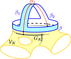
(a) $\alpha_{1}$ connects on component to itself.

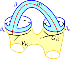
(b) $\alpha_{1}$ connects two different components.

Figure 8. Illustration of the topological situations encountered in the proof of 6.10, when adding a segment $\alpha_{1}$ to the graph $G_{K}$.

• The exit points $o_{1}$ and $e_{1}$ of $\alpha_{1}$ belong to the same connected component $\beta$ of $\partial\mathcal{V}_{K}$, as represented in Figure 8(a). Then, since the path $\tilde{\alpha}_{1}$ is entirely included the complement of $\mathcal{V}_{K}$, the path $\tilde{\alpha}_{1}$ is on the same side of $\beta$ at its two extremities. The regular neighbourhood of $\beta$ and $\tilde{\alpha}_{1}$ is therefore a pair of pants, with three boundary components which we call $\beta^{\prime}$ (for the one freely homotopic to $\beta$), $\beta_{1}$ and $\beta_{2}$.

  • If $\beta_{1}$ or $\beta_{2}$ is contractible, then $\tilde{\alpha}_{1}$ is homotopic with fixed endpoints to a path on $\beta$, and hence $\alpha_{1}$ to one on $G_{K}$.

  • Otherwise, we define $G_{K+1}$ by adding the path $\alpha_{1}$ and its endpoints to the graph $G_{K}$. $G_{K+1}$ automatically satisfies the first condition of (A). For the second condition, we observe that a regular neighbourhood $\mathcal{V}_{K+1}$ of $G_{K+1}$ can be obtained by gluing the pair of pants delimited by $\beta$, $\beta_{1}$ and $\beta_{2}$ to the regular neighbourhood $\mathcal{V}_{K}$ along its boundary component $\beta$. Neither $\beta_{1}$ nor $\beta_{2}$ is contractible, so when we add the disks and cylinders to $\mathcal{V}_{K+1}$ to construct $\mathcal{V}_{K+1}^{+}$, we obtain $\mathcal{V}_{K}^{+}$ together with an additional pair of pants (when $\beta_{1}$ and $\beta_{2}$ are in two different free homotopy classes) or once-holed torus (when $\beta_{1}$ and $\beta_{2}$ are freely homotopic to one another, and hence bound a cylinder). In both cases, $\chi_{\mathcal{V}_{K+1}^{+}}=-(K+1)$ by additivity of the Euler characteristic. Since the boundary of $\mathcal{V}_{K+1}^{+}$ is obtained by taking the boundary of $\mathcal{V}_{K}^{+}$ and either removing the component $\beta$ and adding $\beta_{1}$ and $\beta_{2}$ in the pair of pants case, or just removing $\beta$ in the once-holed torus case,

    $$\ell(\partial\mathcal{V}_{K+1}^{+})\leq\ell(\partial\mathcal{V}_{K}^{+})-\ell(\beta)+\ell(\beta_{1})+\ell(\beta_{2}).$$

    By hypothesis on $\mathcal{V}_{K}^{+}$, its boundary length is $<(K+1)L$. Furthermore, because the pair of pants delimited by $\beta$, $\beta_{1}$ and $\beta_{2}$ is filled by the family of curves $\beta$ and $\tilde{\alpha}_{1}$, of total length $<\ell(\beta)+L/2$, we can pick $\beta_{1}$ and $\beta_{2}$ such that

    $$\ell(\beta)+\ell(\beta_{1})+\ell(\beta_{2})<2\ell(\beta)+L.$$

    As a consequence, $\ell(\partial\mathcal{V}_{K+1}^{+})<(K+2)L$.

• Or the exit points $o_{1}$ and $e_{1}$ belong to two different connected components $\beta_{o}$ and $\beta_{e}$ of $\partial\mathcal{V}_{K}$, like in Figure 8(b). Then, once again, the regular neighbourhood of $\beta_{o}$, $\beta_{e}$ and $\tilde{\alpha}_{1}$ is a pair of pants of boundary components $\beta_{o}^{\prime}$, $\beta_{e}^{\prime}$ and $\beta$.

  • If $\beta$ is contractible, then $\beta_{o}$ and $\beta_{e}$ bound a cylinder $\mathcal{C}$. We modify the definition of $G_{K}$ and replace it by the graph $G_{K}^{\prime}$ obtained by adding the path $\alpha_{1}$ and its endpoints to $G_{K}$. We notice that, when constructing $\mathcal{V}_{K}^{+}$, we would add the cylinder $\mathcal{C}$ to $\mathcal{V}_{K}$. Now, when constructing the new $(\mathcal{V}_{K}^{\prime})^{+}$ from $\mathcal{V}_{K}^{\prime}$, we rather add the contractible boundary component delimited by $\beta$. Hence, the set $(\mathcal{V}_{K}^{\prime})^{+}$ coincides with $\mathcal{V}_{K}^{+}$, and satisfies (A).

  • Otherwise, $\beta$ is not contractible. We add the edge $\alpha_{1}$ and its endpoints to $G_{K}$ and obtain a graph $G_{K+1}$. The regular neighbourhood $\mathcal{V}_{K+1}$ is then obtained by gluing the pair of pants delimited by $\beta_{o}$, $\beta_{e}$, $\beta$ on $\mathcal{V}_{K}$, and $\mathcal{V}_{K+1}^{+}$ is obtained from $\mathcal{V}_{K}^{+}$ by the same process since $\beta$ is not contractible. Hence, the Euler characteristic of $\mathcal{V}_{K+1}^{+}$ is $-(K+1)$, and

    $$\ell(\partial\mathcal{V}_{K+1}^{+})=\ell(\partial\mathcal{V}_{K}^{+})-\ell(\beta_{o})-\ell(\beta_{e})+\ell(\beta)$$

    can be assumed to be $<(K+2)L$ because we can assume that

    $$\ell(\beta_{o})+\ell(\beta_{e})+\ell(\beta)<2\ell(\beta_{o})+2\ell(\beta_{e})+L.$$

In all these cases, we obtain a new family of graphs $(G_{k}^{\prime})_{0\leq k\leq K^{\prime}}$, with $K^{\prime}=K$ or $K+1$, satisfying the hypotheses (A) and (B) for $\gamma_{0},\ldots,\gamma_{j-1}$, and such that the path $\alpha_{1}$ is homotopic with fixed endpoints to a path on $G_{K^{\prime}}^{\prime}$.

We apply this construction successively to $\alpha_{i}$ for $i\in\{1,\ldots,n\}$. At the end, we obtain a family of graphs $(G_{k}^{\prime\prime})_{0\leq k\leq K^{\prime\prime}}$, $K\leq K^{\prime\prime}\leq K+n$, satisfying the hypotheses (A) and (B) for the loops $\gamma_{0},\ldots,\gamma_{j}$, which concludes this step of the iterative construction. ∎

This concludes the proof of 6.9. Then, 6.8 comes as an immediate consequence of the following lemma.

Lemma 6.11.

Let $N\geq 1$ and $L>0$. Let $X=\faktor{\mathcal{H}}{\Gamma}$ be a $(N,L)$-tangle-free hyperbolic surface. Let $\beta$ be a geodesic path of length $\ell$ on $\mathcal{H}$. Then, there exists a neighbourhood $\mathcal{U}$ of $\beta$ in $\mathcal{H}$ and a subgroup $\Gamma_{\mathcal{U}}$ of $\Gamma$ of rank $\mathcal{O}\left(\frac{\ell}{L}\left(\frac{\ell}{L}+N\right)\right)$ such that

$$\forall z\in\mathcal{U},\quad\{\gamma\in\Gamma\,:\,\gamma\cdot z\in\mathcal{U}\}\subset\Gamma_{\mathcal{U}}.$$

Remark 6.12.

The proof actually implies that we can take $\mathcal{U}$ to be equal to the $L/16$-neighbourhood of $\beta$ in $\mathcal{H}$. As a consequence, 6.8 still holds if we replace $S(\gamma)$ by the surface filled by any multi-loop $(\gamma,\beta_{1},\ldots,\beta_{n})$, where $(\beta_{i})_{i}$ is a family of geodesic paths of length $\leq L/16$ that each intersect $\gamma$.

Proof.

Let us cover the geodesic $\beta$ by $k=\mathcal{O}\left(\frac{\ell}{L}\right)$ balls of radius $\frac{L}{8}$, centered at points denoted by $z_{1},\ldots,z_{k}$. Then, the open sets

$$\mathcal{U}:=\bigcup_{i=1}^{k}\mathcal{B}_{\frac{L}{8}}(z_{i})\qquad\text{and}\qquad\mathcal{U}_{+}:=\bigcup_{i=1}^{k}\mathcal{B}_{\frac{L}{4}}(z_{i}).$$

are neighbourhoods of the curve $\beta$.

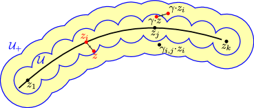
Figure 9. Illustration of the proof of 6.11.

For each index $i\in\{1,\ldots,k\}$, we set $\Gamma_{i}(\mathcal{U}_{+}):=\{\gamma\in\Gamma\,:\,\gamma\cdot z_{i}\in\mathcal{U}_{+}\}$. We claim that

$$\forall z\in\mathcal{U},\quad\{\gamma\in\Gamma\,:\,\gamma\cdot z\in\mathcal{U}\}\subset\bigcup_{i=1}^{k}\Gamma_{i}(\mathcal{U}_{+}).$$

Indeed, any element $z$ of $\mathcal{U}$ belongs in $\mathcal{B}_{\frac{L}{8}}(z_{i})$ for an integer $i$. For an element $\gamma\in\Gamma$, if $\gamma\cdot z\in\mathcal{U}$, then there is an index $j$ such that $\gamma\cdot z\in\mathcal{B}_{\frac{L}{8}}(z_{j})$. Then,

$$\operatorname{dist}_{\mathcal{H}}(z_{j},\gamma\cdot z_{i})\leq\operatorname{dist}_{\mathcal{H}}(z_{j},\gamma\cdot z)+\operatorname{dist}_{\mathcal{H}}(\gamma\cdot z,\gamma\cdot z_{i})<\frac{L}{8}+\frac{L}{8}=\frac{L}{4}$$

and therefore $\gamma\cdot z_{i}\in\mathcal{B}_{\frac{L}{4}}(z_{j})\subset\mathcal{U}_{+}$, which implies that $\gamma\in\Gamma_{i}(\mathcal{U}_{+})$.

Therefore, we only need to prove that for all $i\in\{1,\ldots,k\}$, the set $\Gamma_{i}(\mathcal{U}_{+})$ is included in a subgroup of $\Gamma$ of rank $\mathcal{O}\left(\frac{\ell}{L}+N\right)$ using the $(N,L)$-tangle-free hypothesis. This will lead to the conclusion because $k=\mathcal{O}\left(\frac{\ell}{L}\right)$.

For each $j\neq i$, let us pick a $\gamma_{i,j}\in\Gamma$ such that $\gamma_{i,j}\cdot z_{i}\in\mathcal{B}_{\frac{L}{4}}(z_{j})$, provided such a transformation exists. Then, if $\gamma\in\Gamma_{i}(\mathcal{U}_{+})$, $\gamma\cdot z_{i}\in\mathcal{U}_{+}$ so one of the following occurs:

• either $\gamma\cdot z_{i}\in\mathcal{B}_{\frac{L}{4}}(z_{i})$, which implies that $\gamma\in\Gamma_{\frac{L}{4}}(z_{i})\subset\Gamma_{\frac{L}{2}}(z_{i})$;

• or $\gamma\cdot z_{i}\in\mathcal{B}_{\frac{L}{4}}(z_{j})$ for a $j\neq i$, and hence

  $$\operatorname{dist}_{\mathcal{H}}(\gamma_{i,j}\cdot z_{i},\gamma\cdot z_{i})\leq\operatorname{dist}_{\mathcal{H}}(\gamma_{i,j}\cdot z_{i},z_{j})+\operatorname{dist}_{\mathcal{H}}(z_{j},\gamma\cdot z_{i})<\frac{L}{4}+\frac{L}{4}=\frac{L}{2}$$

  so $\gamma_{i,j}^{-1}\gamma$ is an element of $\Gamma_{\frac{L}{2}}(z_{i})$.

As a consequence, every element of $\Gamma_{i}(\mathcal{U}_{+})$ can be written as a product of the $(\gamma_{i,j})_{j\neq i}$ and the elements of $\Gamma_{\frac{L}{2}}(z_{i})$. The latter is included in a sub-group of $\Gamma$ of rank $\leq N$ by the tangle-free hypothesis and 6.9, while the former contains $k-1$ elements. Therefore, $\Gamma_{i}(\mathcal{U}_{+})$ is included in a sub-group of rank $\leq N+k-1$, which allows us to conclude. ∎

7. The case of the figure-eight

The aim of this section is to prove Objective (FR) in the case of a figure-eight in a pair of pants, which is the local topological type represented in Figure 10.

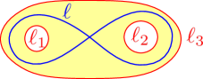
Figure 10. A figure-eight in a pair of pants.

The figure-eight is the simplest example of loop filling the pair of pants, which is why we address it first. We prove the following.

Theorem 7.1.

Let $\alpha$ be a figure-eight filling a pair of pants $P$, and $T=[P,\alpha]_{\mathrm{loc}}$. Then, for all $k\geq 0$, the function $f_{k}^{T}$ is a Friedman–Ramanujan function.

By “simplest”, we mean that it is the loop with the least self-intersections filling $P$, as opposed to more complicated loops such as the one represented in the left part of Figure 3(b). However, when we prove Objective (FR) for all other loops filling $P$ in Section 8, we will notice that it is actually the one for which the analysis is the hardest.

7.1. Expression of the density function as an integral

Let $F:\mathbb{R}_{\geq 0}\rightarrow\mathbb{R}$ be an admissible function. We recall that, by definition, the functions $f_{k}^{T}$ will appear when computing the asymptotic expansion of the average

$$\langle F\rangle_{g}^{{T}}=\mathbb{E}_{g}^{\mathrm{\scriptsize{WP}}}\Bigg{[}\sum_{\gamma\in T^{g}}F(\ell_{X}(\gamma))\Bigg{]}.$$

We saw in 5.5 that this expectation can be expressed as

(7.1) $$\langle F\rangle_{g}^{{T}}=\iiint_{\mathbb{R}_{>0}^{3}}F(\mathfrak{L}(\ell_{1},\ell_{2},\ell_{3}))\,\phi_{g}^{P}(\ell_{1},\ell_{2},\ell_{3})\,\,\mathrm{d}\ell_{1}\,\mathrm{d}\ell_{2}\,\mathrm{d}\ell_{3},$$

where

• $\phi_{g}^{P}$ is the sum over all realisations of the pair of pants, defined in (5.4) and computed in 5.7;

• the length function $\mathfrak{L}:\mathbb{R}_{>0}^{3}\rightarrow\mathbb{R}_{>0}$ associates to $(\ell_{1},\ell_{2},\ell_{3})$ the length of the figure-eight going around the components $1$ and $2$ in the pair of pants of boundary components of lengths $\ell_{1},\ell_{2},\ell_{3}$. It is computed in [7, equation 4.2.3]:

  (7.2) $$\cosh\left(\frac{\mathfrak{L}(\ell_{1},\ell_{2},\ell_{3})}{2}\right)=2\cosh\left(\frac{\ell_{1}}{2}\right)\cosh\left(\frac{\ell_{2}}{2}\right)+\cosh\left(\frac{\ell_{3}}{2}\right).$$

By 5.21, the function $\phi_{g}^{P}(\ell_{1},\ell_{2},\ell_{3})$ has an expansion in powers of $1/g$. The dependency of its terms with respect to $(\ell_{i})_{1\leq i\leq 3}$ is detailed. When substituting $\phi_{g}^{P}$ by its expansion in (7.1), we obtain that any term of the asymptotic expansion of the average $\langle F\rangle_{g}^{{T}}$ in powers of $1/g$ is a linear combination of integrals of the form

(7.3) $$\iiint_{\mathbb{R}_{>0}^{3}}F(\mathfrak{L}(\ell_{1},\ell_{2},\ell_{3}))\,\prod_{i=1}^{3}h_{i}(\ell_{i})\,\,\mathrm{d}\ell_{1}\,\mathrm{d}\ell_{2}\,\mathrm{d}\ell_{3}$$

(7.4) $$\iiint_{\mathbb{R}_{>0}^{3}}F(\mathfrak{L}(\ell_{1},\ell_{2},\ell_{3}))\,h_{i}(\ell_{i})\,\ell_{j}\delta(\ell_{j}-\ell_{k})\,\mathrm{d}\ell_{1}\,\mathrm{d}\ell_{2}\,\mathrm{d}\ell_{3}\quad\text{for }\{i,j,k\}=\{1,2,3\}$$

where for all $i$, the functions $\ell_{i}\mapsto h_{i}(\ell_{i})$ is of the form

(7.5) $$\ell_{i}^{2k+1}\quad\text{or}\quad\ell_{i}^{2k+1}\cosh\left(\frac{\ell_{i}}{2}\right)\quad\text{or}\quad\ell_{i}^{2k}\sinh\left(\frac{\ell_{i}}{2}\right).$$

7.2. Level-set decomposition

Because we want to view the average $\langle F\rangle_{g}^{{T}}$ as the integral of $F$ against a density, we rewrite the integral (7.3) as

$$\int_{0}^{+\infty}F(\ell)\left(\iint_{\mathfrak{L}(\ell_{1},\ell_{2},\ell_{3})=\ell}\,\prod_{i=1}^{3}h_{i}(\ell_{i})\,\frac{\,\mathrm{d}\ell_{1}\,\mathrm{d}\ell_{2}\,\mathrm{d}\ell_{3}}{\,\mathrm{d}\ell}\right)\,\mathrm{d}\ell.$$

Let us give precise meaning to this writing. We fix $\ell_{1},\ell_{2}>0$. Then, the application

$$\mathfrak{L}_{\ell_{1},\ell_{2}}:\begin{cases}\mathbb{R}_{>0}\rightarrow I(\ell_{1},\ell_{2})\\ \ell_{3}\hskip 5.0pt\mapsto\mathfrak{L}(\ell_{1},\ell_{2},\ell_{3})=2\operatorname{argch}\left(2\cosh\left(\frac{\ell_{1}}{2}\right)\cosh\left(\frac{\ell_{2}}{2}\right)+\cosh\left(\frac{\ell_{3}}{2}\right)\right)\end{cases}$$

is a diffeomorphism from $\mathbb{R}_{>0}$ to an interval $I(\ell_{1},\ell_{2})$ of $\mathbb{R}_{>0}$. We introduce the following notation.

Notation 7.2.

Let $\ell>0$. For any integrable function $G:\mathbb{R}_{>0}^{3}\rightarrow\mathbb{C}$, we define

$$\iint_{\mathfrak{L}(\ell_{1},\ell_{2},\ell_{3})=\ell}G(\ell_{1},\ell_{2},\ell_{3})\,\frac{\,\mathrm{d}\ell_{1}\,\mathrm{d}\ell_{2}\,\mathrm{d}\ell_{3}}{\,\mathrm{d}\ell}:=\iint_{\mathbb{R}_{>0}^{2}}\frac{\mathds{1}_{I(\ell_{1},\ell_{2})}(\ell)\,G(\ell_{1},\ell_{2},\mathfrak{L}_{\ell_{1},\ell_{2}}^{-1}(\ell))}{\mathfrak{L}^{\prime}_{\ell_{1},\ell_{2}}(\mathfrak{L}_{\ell_{1},\ell_{2}}^{-1}(\ell))}\,\mathrm{d}\ell_{1}\,\mathrm{d}\ell_{2}.$$

This formula corresponds to considering the variable $\ell_{3}$ as a function of the variables $\ell_{1},\ell_{2},\ell$, once restricted to the $2$-dimensional level-set $\{(\ell_{1},\ell_{2},\ell_{3})\;:\;\mathfrak{L}(\ell_{1},\ell_{2},\ell_{3})=\ell\}$. The derivative that appears corresponds, formally, to writing

$$\frac{\,\mathrm{d}\ell_{1}\,\mathrm{d}\ell_{2}\,\mathrm{d}\ell_{3}}{\,\mathrm{d}\ell}=\frac{\partial\ell_{3}}{\partial\ell}(\ell_{1},\ell_{2},\ell)\,\mathrm{d}\ell_{1}\,\mathrm{d}\ell_{2}.$$

It is easy to check using the local inversion theorem that one obtains the same quantity by performing this operation on the variables $\ell_{2}$ and $\ell_{3}$, or $\ell_{1}$ and $\ell_{3}$.

We do the same for the integrals of the form (7.4). For instance, for $(i,j,k)=(1,2,3)$, we obtain the integral

(7.6) $$\int_{\mathfrak{L}(\ell_{1},\ell_{2},\ell_{2})=\ell}h_{1}(\ell_{1})\,\ell_{2}\,\frac{\,\mathrm{d}\ell_{1}\,\mathrm{d}\ell_{2}}{\,\mathrm{d}\ell}\cdot$$

7.3. Reformulation of the question and proof in simple cases

It will be handy to observe that, for any of the three cases in (7.5), we can write

$$f_{i}(\ell_{i}):=\frac{h_{i}(\ell_{i})}{\sinh\left(\frac{\ell_{i}}{2}\right)}=p_{i}(\ell_{i})+\mathcal{O}\left((\ell_{i}+1)^{c_{i}}\exp\left(-\frac{\ell_{i}}{2}\right)\right)$$

where $p_{i}$ is a polynomial function (possibly equal to zero) and $c_{i}\geq 0$, because

$$\frac{\ell_{i}}{\sinh\left(\frac{\ell_{i}}{2}\right)}=\mathcal{O}\left((\ell_{i}+1)\,e^{-\frac{\ell_{i}}{2}}\right)\quad\text{and}\quad\cosh\left(\frac{\ell_{i}}{2}\right)=\sinh\left(\frac{\ell_{i}}{2}\right)+e^{-\frac{\ell_{i}}{2}}.$$

All of the steps taken so far lead us to the following lemma.

Lemma 7.3.

For any integer $k\geq 0$, the function $\ell\mapsto f_{k}^{T}(\ell)$ is a linear combination of functions of the form

(7.7) $$\mathcal{I}[f_{1},f_{2},f_{3}]:\ell\mapsto\iint_{\mathfrak{L}(\ell_{1},\ell_{2},\ell_{3})=\ell}\,\prod_{i=1}^{3}f_{i}(\ell_{i})\sinh\left(\frac{\ell_{i}}{2}\right)\,\frac{\,\mathrm{d}\ell_{1}\,\mathrm{d}\ell_{2}\,\mathrm{d}\ell_{3}}{\,\mathrm{d}\ell}$$

and

(7.8) $$\begin{cases}&\mathcal{I}^{\mathrm{tor}}_{1}[f_{1}]:\ell\mapsto\int_{\mathfrak{L}(\ell_{1},\ell_{2},\ell_{2})=\ell}\,f_{1}(\ell_{1})\sinh\left(\frac{\ell_{1}}{2}\right)\,\ell_{2}\,\frac{\,\mathrm{d}\ell_{1}\,\mathrm{d}\ell_{2}}{\,\mathrm{d}\ell}\\ &\mathcal{I}^{\mathrm{tor}}_{2}[f_{2}]:\ell\mapsto\int_{\mathfrak{L}(\ell_{3},\ell_{2},\ell_{3})=\ell}\,f_{2}(\ell_{2})\sinh\left(\frac{\ell_{2}}{2}\right)\,\ell_{3}\,\frac{\,\mathrm{d}\ell_{2}\,\mathrm{d}\ell_{3}}{\,\mathrm{d}\ell}\\ &\mathcal{I}^{\mathrm{tor}}_{3}[f_{3}]:\ell\mapsto\int_{\mathfrak{L}(\ell_{1},\ell_{1},\ell_{3})=\ell}\,f_{3}(\ell_{3})\sinh\left(\frac{\ell_{3}}{2}\right)\,\ell_{1}\,\frac{\,\mathrm{d}\ell_{1}\,\mathrm{d}\ell_{3}}{\,\mathrm{d}\ell}\end{cases}$$

where for any $i\in\{1,2,3\}$, $f_{i}$ satisfies:

(7.9) $$|f_{i}(\ell_{i})-p_{i}(\ell_{i})|\leq c_{i}(\ell_{i}+1)^{c_{i}}\exp\left(-\frac{\ell_{i}}{2}\right)$$

for a polynomial function $p_{i}$ and a constant $c_{i}>0$.

In particular, if we prove that the integrals in (7.7) and (7.8) are Friedman–Ramanujan for any $(f_{i})_{1\leq i\leq 3}$ satisfying (7.9), then we can conclude that $f_{k}^{T}$ is too, by linearity, hence proving 7.1. Let us prove this in some simple cases.

Lemma 7.4.

Let $(f_{i})_{1\leq i\leq 3}$ be measurable functions, each satisfying (7.9).

1. If $p_{1}=p_{2}=0$, then $\mathcal{I}[f_{1},f_{2},f_{3}]\in\mathcal{R}\subset\mathcal{F}$.

2. If $p_{3}=0$, then $\mathcal{I}[f_{1},f_{2},f_{3}]\in\mathcal{R}\subset\mathcal{F}$.

3. Without any further hypothesis, the integrals in (7.8) belong in $\mathcal{R}\subset\mathcal{F}$.

Proof.

Before we proceed to the proof, let us observe that

(7.10) $$\ell_{1}+\ell_{2}\leq\ell\quad\text{and}\quad\ell_{3}\leq\ell.$$

This can be seen on the expressions, or directly on Figure 10, by minimality of the length of a geodesic in a free homotopy class.

The proof of 7.4 for all integrals of the form (7.8) are similar, and we therefore detail the computation for $\mathcal{I}_{1}^{\mathrm{tor}}$ only. First, we use the level-set condition

$$\cosh\left(\frac{\ell}{2}\right)=\cosh\left(\frac{\ell_{2}}{2}\right)\left(2\cosh\left(\frac{\ell_{1}}{2}\right)+1\right)$$

to compute that

$$\frac{\partial\ell_{1}}{\partial\ell}=\frac{\sinh\left(\frac{\ell}{2}\right)}{2\sinh\left(\frac{\ell_{1}}{2}\right)\cosh\left(\frac{\ell_{2}}{2}\right)}\leq\frac{\sinh\left(\frac{\ell}{2}\right)}{\sinh\left(\frac{\ell_{1}}{2}\right)}\cdot$$

The hypothesis (7.9) on $f_{1}$ implies that there exists a constant $c>0$ such that

$$|f_{1}(\ell_{1})|\leq c(\ell_{1}+1)^{c}.$$

It follows, using (7.10), that

$$\left|f_{1}(\ell_{1})\sinh\left(\frac{\ell_{1}}{2}\right)\ell_{2}\frac{\partial\ell_{1}}{\partial\ell}\right|\leq c(\ell+1)^{c+1}\sinh\left(\frac{\ell}{2}\right)$$

and hence

$$|\mathcal{I}^{\mathrm{tor}}_{1}[f_{1}](\ell)|\leq c(\ell+1)^{c+1}\sinh\left(\frac{\ell}{2}\right)\int_{0}^{\ell}\,\mathrm{d}\ell_{2}\leq c(\ell+1)^{c+2}\exp\left(\frac{\ell}{2}\right)$$

which means that $\ell\mapsto\mathcal{I}^{\mathrm{tor}}_{1}[f_{1}](\ell)$ belongs in $\mathcal{R}$.

Let us now treat case when $p_{3}=0$. In that case, now using

$$\cosh\left(\frac{\ell}{2}\right)=2\cosh\left(\frac{\ell_{1}}{2}\right)\cosh\left(\frac{\ell_{2}}{2}\right)+\cosh\left(\frac{\ell_{3}}{2}\right),$$

we obtain

(7.11) $$\frac{\partial\ell_{2}}{\partial\ell}=\frac{\sinh\left(\frac{\ell}{2}\right)}{2\cosh\left(\frac{\ell_{1}}{2}\right)\sinh\left(\frac{\ell_{2}}{2}\right)}\cdot$$

We then observe that our assumptions on $(f_{i})_{1\leq i\leq 3}$ implies that there exists a constant $c\geq 0$ such that, for any $\ell_{1},\ell_{3},\ell$ for which $\ell_{2}$ is well-defined,

(7.12) $$\left|\prod_{i=1}^{3}f_{i}(\ell_{i})\sinh\left(\frac{\ell_{i}}{2}\right)\,\frac{\partial\ell_{2}}{\partial\ell}\right|\leq c(\ell_{1}+\ell_{2}+\ell_{3}+1)^{c}\sinh\left(\frac{\ell}{2}\right).$$

which, by (7.10), implies

$$\mathcal{I}[f_{1},f_{2},f_{3}](\ell)=\mathcal{O}\left((\ell+1)^{c}\sinh\left(\frac{\ell}{2}\right)\iint_{[0,\ell]^{2}}\,\mathrm{d}\ell_{1}\,\mathrm{d}\ell_{3}\right)=\mathcal{O}\left((\ell+1)^{c+2}\exp\left(\frac{\ell}{2}\right)\right),$$

which is our claim.

The proof the remaining case is the same, now expressing $\ell_{3}$ in terms of $\ell_{1},\ell_{2}$ and $\ell$. Indeed,

$$\frac{\partial\ell_{3}}{\partial\ell}=\frac{\sinh\left(\frac{\ell}{2}\right)}{\sinh\left(\frac{\ell_{3}}{2}\right)}$$

and hence $\prod_{i=1}^{3}f_{i}(\ell_{i})\sinh\left(\frac{\ell_{i}}{2}\right)\,\frac{\partial\ell_{3}}{\partial\ell}$ satisfies the bound (7.12) when $p_{1}=p_{2}=0$. ∎

Remark 7.5.

The fact that we obtain a function in $\mathcal{R}$ in cases (1) and (2) corresponds to the fact that, if $\tilde{f}_{1},\tilde{f}_{2}\in\mathcal{R}$, then $\tilde{f}_{1}\star\tilde{f}_{2}\in\mathcal{R}$, as observed in the proof of the stability of $\mathcal{F}$ by convolution (3.5), which we invite the reader to read at this stage. Another insight that one can gather from proof is that, if $\tilde{f}_{1},\tilde{f}_{2}\in\mathcal{F}$ are of respective main terms $\tilde{p}_{1},\tilde{p}_{2}$, then the main term of $\tilde{f}_{1}\star\tilde{f}_{2}$ is not only $\tilde{p}_{1}\star\tilde{p}_{2}$, but actually contains contributions coming from the remainders terms of $\tilde{f}_{1},\tilde{f}_{2}$. This is the reason why 7.4 only holds if both $f_{1}$ and $f_{2}$ have no polynomial term, and not when only one of them does. We do expect the contributions where $p_{1}\neq 0$ whilst $p_{2}=0$ to participate to the main term of $\mathcal{I}[f_{1},f_{2},f_{3}]$.

7.4. Change of variables

In order to study the integrals $\mathcal{I}[f_{1},f_{2},f_{3}]$ more precisely, it will be helpful to introduce new variables, which transform the level-set integral (7.7) into a convolution-like integral. We shall use the following new variables, which are represented in Figure 11:

• $L_{1}$ and $L_{2}$ denote the lengths of the geodesic arcs based at the self-intersection of $\alpha$, going around the first and second boundary components of the pair of pants respectively;

• $u:=\cos^{2}\left(\frac{\theta}{2}\right)$, where $\theta$ denotes the outer angle of the self-intersection of $\alpha$.

We observe that, in these new coordinates, we always have $\mathfrak{L}(\ell_{1},\ell_{2},\ell_{3})=L_{1}+L_{2}$, and hence the level-set integral is an integral on $\{(L_{1},L_{2},u)\in\mathbb{R}_{>0}^{2}\times(0,1)\,:\,L_{1}+L_{2}=\ell\}$, similar to a convolution. This is evocative of the case of graphs, described in Section 3.3. A significant difference with the case of graphs is the presence of an additional parameter $u\in(0,1)$ that is required to describe the geometry of the pair of pants; in the following, this quantity will mostly behave like a free parameter in $(0,1)$ that we will integrate out.

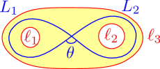
Figure 11. The new variables $(L_{1},L_{2},u=\cos^{2}(\theta/2))$ used to describe the geometry of the pair of pants.

The following lemma provides an expression for the lengths $\ell_{1},\ell_{2},\ell_{3}$ of the three boundary components of the pair of pants, in terms of the new variables $(L_{1},L_{2},u)$.

Lemma 7.6.

For any $\ell_{1},\ell_{2},\ell_{3}>0$,

(7.14)

Proof.

Let $z$ denote the intersection point of the figure eight, and $\alpha_{1}$ denote the portion of $\alpha$ going around the first boundary component, $b_{1}$, of $P$. We draw the common perpendicular of $\alpha_{1}$ and $b_{1}$, as well as the perpendicular of $b_{1}$ passing through $z$. When cutting along $\alpha_{1}$ and those two perpendiculars, we obtain a trirectangle, represented in Figure 12. By [7, Theorem 2.3.1(iii)],

$$\cosh\left(\frac{\ell_{1}}{2}\right)=\sin\left(\frac{\pi-\theta}{2}\right)\cosh\left(\frac{L_{1}}{2}\right)=\sqrt{u}\cosh\left(\frac{L_{1}}{2}\right),$$

and same goes for $\ell_{2}$.

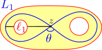
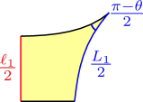
Figure 12. Illustration of the proof of 7.6.

The formula for $\ell_{3}$ is obtained directly from the formula for the length of the figure eight,

$$\cosh\left(\frac{L_{1}+L_{2}}{2}\right)=2\cosh\left(\frac{\ell_{1}}{2}\right)\cosh\left(\frac{\ell_{2}}{2}\right)+\cosh\left(\frac{\ell_{3}}{2}\right)$$

together with the fact that, by (7.6),

$$2\cosh\left(\frac{\ell_{1}}{2}\right)\cosh\left(\frac{\ell_{2}}{2}\right)=2u\cosh\left(\frac{L_{1}}{2}\right)\cosh\left(\frac{L_{2}}{2}\right)$$

and we have the usual trigonometric formula

$$2\cosh\left(\frac{L_{1}}{2}\right)\cosh\left(\frac{L_{2}}{2}\right)=\cosh\left(\frac{L_{1}+L_{2}}{2}\right)+\cosh\left(\frac{L_{1}-L_{2}}{2}\right).$$

∎

This is enough to entirely describe the change of variable $(\ell_{1},\ell_{2},\ell_{3})\rightarrow(L_{1},L_{2},u)$, which we do in the following lemma.

Lemma 7.7.

The application $(\ell_{1},\ell_{2},\ell_{3})\mapsto(L_{1},L_{2},u)$ is a diffeomorphism from the set $\mathbb{R}_{>0}^{3}$ onto the set $\mathcal{E}\subset\mathbb{R}_{>0}^{2}\times(0,1)$ defined by

(7.15) $$\mathcal{E}:=\left\{(L_{1},L_{2},u)\,:\,\begin{cases}\sqrt{u}\cosh\left(\frac{L_{i}}{2}\right)>1\qquad\text{for }i\in\{1,2\}\\ (1-u)\cosh\left(\frac{L_{1}+L_{2}}{2}\right)>u\cosh\left(\frac{L_{1}-L_{2}}{2}\right)+1\end{cases}\right\},$$

and we have that

$$\,\mathrm{d}\ell_{1}\,\mathrm{d}\ell_{2}\,\mathrm{d}\ell_{3}=-\dfrac{\sinh\left(\frac{L_{1}+L_{2}}{2}\right)^{2}}{\sinh\left(\frac{\ell_{1}}{2}\right)\sinh\left(\frac{\ell_{2}}{2}\right)\sinh\left(\frac{\ell_{3}}{2}\right)}\,\mathrm{d}L_{1}\,\mathrm{d}L_{2}\,\mathrm{d}u.$$

Proof.

The first part of the statement is a straightforward consequence of 7.6 together with the fact that $\cosh:(0,+\infty)\rightarrow(1,+\infty)$ is a diffeomorphism. The only thing we need to check is the expression for the Jacobian of the change of variable. Using 7.6, we compute the partial derivatives of $\ell_{1},\ell_{2},\ell_{3}$ expressed as functions of $L_{1},L_{2},u$, using the slight variation of (7.14)

$$\cosh\left(\frac{\ell_{3}}{2}\right)=\cosh\left(\frac{L_{1}+L_{2}}{2}\right)-2u\cosh\left(\frac{L_{1}}{2}\right)\cosh\left(\frac{L_{2}}{2}\right).$$

We obtain that we need to compute the determinant

$$\frac{1}{\prod_{i=1}^{3}\sinh\left(\frac{\ell_{i}}{2}\right)}\begin{vmatrix}\sqrt{u}\sinh\left(\frac{L_{1}}{2}\right)&0&\sinh\left(\frac{L_{1}+L_{2}}{2}\right)-2u\sinh\left(\frac{L_{1}}{2}\right)\cosh\left(\frac{L_{2}}{2}\right)\\ 0&\sqrt{u}\sinh\left(\frac{L_{2}}{2}\right)&\sinh\left(\frac{L_{1}+L_{2}}{2}\right)-2u\cosh\left(\frac{L_{1}}{2}\right)\sinh\left(\frac{L_{2}}{2}\right)\\ \frac{1}{\sqrt{u}}\cosh\left(\frac{L_{1}}{2}\right)&\frac{1}{\sqrt{u}}\cosh\left(\frac{L_{2}}{2}\right)&-4\cosh\left(\frac{L_{1}}{2}\right)\cosh\left(\frac{L_{2}}{2}\right)\end{vmatrix}.$$

We add $2\sqrt{u}\cosh\left(\frac{L_{2}}{2}\right)$ times the first column and $2\sqrt{u}\cosh\left(\frac{L_{1}}{2}\right)$ times the second column to the third, which removes its negative terms. We then factor out the $\sinh\left(\frac{L_{1}+L_{2}}{2}\right)$ in the third column, and obtain the determinant

$$\frac{\sinh\left(\frac{L_{1}+L_{2}}{2}\right)}{\prod_{i=1}^{3}\sinh\left(\frac{\ell_{i}}{2}\right)}\begin{vmatrix}\sqrt{u}\sinh\left(\frac{L_{1}}{2}\right)&0&1\\ 0&\sqrt{u}\sinh\left(\frac{L_{2}}{2}\right)&1\\ \frac{1}{\sqrt{u}}\cosh\left(\frac{L_{1}}{2}\right)&\frac{1}{\sqrt{u}}\cosh\left(\frac{L_{2}}{2}\right)&0\end{vmatrix}=-\frac{\sinh^{2}\left(\frac{L_{1}+L_{2}}{2}\right)}{\prod_{i=1}^{3}\sinh\left(\frac{\ell_{i}}{2}\right)}\cdot$$

∎

7.5. Technical lemmas about the change of variables

In order to prove 7.1, which we shall do in the next section, we need a few technical lemmas describing the change of variable $(\ell_{1},\ell_{2},\ell_{3})\rightarrow(L_{1},L_{2},u)$ more precisely. For that purpose, we introduce the following notations.

Notation 7.8.

We set $\ell_{0}:=4\operatorname{argch}(\sqrt{2})$. For $\ell>0$, we define

(7.16) $$u_{-}(\ell):=\frac{1}{\cosh^{2}\left(\frac{\ell}{4}\right)}\quad\text{and}\quad u_{+}(\ell):=1-\frac{1}{\cosh^{2}\left(\frac{\ell}{4}\right)}$$

and, for any $u\in(0,1)$, we define

$$L_{-}^{\infty}(u):=\max\left(2\operatorname{argch}\left(\frac{1}{\sqrt{u}}\right),\log\left(\frac{u}{1-u}\right)\right).$$

We shall refer to the following two subsets of $\mathbb{R}_{>0}\times(0,1)$:

$$\mathcal{E}_{1} :=\{(\ell,u)\in(\ell_{0},+\infty)\times(0,1)\,:\,u_{-}(\ell)<u<u_{+}(\ell)\}$$

$$\mathcal{E}_{2}^{\infty} :=\{(L,u)\in\mathbb{R}_{>0}\times(0,1)\,:\,L>L_{-}^{\infty}(u)\}.$$

Let us list a few elementary properties of the quantities defined above.

Lemma 7.9.

1. Let $\ell>0$. Then, $u_{-}(\ell)<u_{+}(\ell)$ if and only if $\ell>\ell_{0}$.

2. We have for any $\ell>0$, $\lvert\log(u_{-}(\ell))\rvert=\lvert\log(1-u_{+}(\ell))\rvert\leq\ell/2$. Furthermore, for any integer $m\geq 0$, there exists $C_{m}>0$ such that, for any $\ell>0$,

   (7.17) $$\int_{0}^{u_{-}(\ell)}|\log u|^{m}\,\mathrm{d}u\leq C_{m}(\ell+1)^{m}e^{-\frac{\ell}{2}}.$$

3. The function $u\mapsto L_{-}^{\infty}(u)$ is equivalent to $-\log(u)$ for $u$ close to $0$ and $-\log(1-u)$ for $u$ close to $1$.

Proof.

The first and last points are trivial, and so is the first part of (2). The rest of the second point can be obtained by proving that for any $\epsilon>0$,

$$\int_{0}^{\epsilon}|\log(u)|^{m}\,\mathrm{d}u=\int_{-\log(\epsilon)}^{+\infty}v^{m}e^{-v}\,\mathrm{d}v=\mathcal{O}\left((|\log(\epsilon)|+1)^{m}\epsilon\right)$$

by iterated integration by parts, and then taking $\epsilon=u_{-}(\ell)$. ∎

Let us now provide a finer description of the set $\mathcal{E}$ defined in 7.7.

Lemma 7.10.

For any $\ell>0$, any $u\in(0,1)$, any $L\in(0,\frac{\ell}{2})$,

$$(L,\ell-L,u)\in\mathcal{E}\quad\Leftrightarrow\quad\begin{cases}(\ell,u)\in\mathcal{E}_{1}\\ L>L_{-}(\ell,u)\end{cases}$$

where the function $L_{-}:\mathcal{E}_{1}\rightarrow(0,\frac{\ell}{2})$ satisfies, for a constant $C>0$,

(7.18) $$\forall(\ell,u)\in\mathcal{E}_{1},\quad 0\leq L_{-}(\ell,u)-L_{-}^{\infty}(u)\leq C\ell\frac{e^{-\frac{\ell}{2}}}{1-u}\cdot$$

Note that, here, we are only describing on the part of $\mathcal{E}$ for which $L_{1}<L_{2}$ (which is equivalent to $L_{1}<\ell/2$ since $L_{1}+L_{2}=\ell$). Since $L_{1}$ and $L_{2}$ play symmetric roles, this allows us to describe the entirety of $\mathcal{E}$.

Proof.

Let us consider a $\ell>0$, $0<u<1$, and $0<L<\frac{\ell}{2}$.

The first condition defining $\mathcal{E}$ is $\sqrt{u}\cosh\left(\frac{L}{2}\right)>1$. The existence of number $L$ in $(0,\frac{\ell}{2})$ satisfying this inequality is equivalent to the following condition on $u$ and $\ell$:

$$\sqrt{u}\cosh\left(\frac{\ell}{4}\right)>1\quad\Leftrightarrow\quad u>u_{-}(\ell).$$

Then, $L$ satisfies the condition if and only if

$$L>L^{1}_{-}(u):=2\operatorname{argch}\left(\frac{1}{\sqrt{u}}\right).$$

Now, because we assume that $L<\frac{\ell}{2}$, we have that $\ell-L>L$, and hence the second condition of $\mathcal{E}$ is automatically satisfied once the first is.

Let us now move on the last condition defining $\mathcal{E}$,

$$(1-u)\cosh\left(\frac{\ell}{2}\right)-u\cosh\left(\frac{\ell}{2}-L\right)>1.$$

The left hand side of this equation is an increasing function of $L\in(0,\frac{\ell}{2})$, and is therefore maximal at $\ell/2$. As a consequence, there exists a value $L$ in $(0,\frac{\ell}{2})$ so that it exceeds $1$ if and only if

$$(1-u)\cosh\left(\frac{\ell}{2}\right)-u>1\quad\Leftrightarrow\quad u<u_{+}(\ell).$$

In that case, $L$ satisfies the third condition of $\mathcal{E}$ if and only if

$$L>L^{3}_{-}(\ell,u):=\frac{\ell}{2}-\operatorname{argch}\left(\frac{1-u}{u}\cosh\left(\frac{\ell}{2}\right)-\frac{1}{u}\right).$$

Finally, we observe that we need to have $u_{-}(\ell)<u_{+}(\ell)$ for all three conditions of $\mathcal{E}$ to be satisfied together, which we saw in 7.9 is equivalent to $\ell>\ell_{0}$. Then, we have the claimed result with

$$L_{-}(\ell,u):=\max\left(L^{1}_{-}(u),L^{3}_{-}(\ell,u)\right).$$

To prove the bound on $L_{-}-L_{-}^{\infty}$, we simply need to observe that for $x>1$,

$$\operatorname{argch}(x)=\log\left(x+\sqrt{x^{2}-1}\right)=\log\left(2x+\mathcal{O}\left(1\right)\right)$$

and hence

$$L^{3}_{-}(\ell,u)=\frac{\ell}{2}-\log\left(\frac{1-u}{u}\,e^{\frac{\ell}{2}}+\mathcal{O}\left(\frac{1}{u}\right)\right)=\log\left(\frac{u}{1-u}\right)-\log(1+A(\ell,u))$$

where the quantity $A(\ell,u)>-1$ satisfies $A(\ell,u)=\mathcal{O}\left(e^{-\frac{\ell}{2}}/(1-u)\right)$. There exists a constant $c>0$ such that, for any real number $A\geq-1/2$, $|\log(1+A)|\leq c|A|$. This is enough to conclude whenever $A(\ell,u)\geq-1/2$, since $\ell>\ell_{0}$. Otherwise, we rather use the trivial bound

$$\left|L^{3}_{-}(\ell,u)-\log\left(\frac{u}{1-u}\right)\right|\leq\frac{\ell}{2}+|\log(u_{-}(\ell))|+|\log(1-u_{+}(\ell))|\leq 2\ell.$$

This leads to the claimed estimate, because if $A(\ell,u)<-1/2$, then $e^{-\frac{\ell}{2}}/(1-u)$ is bounded away from $0$. ∎

The next lemma is an expansion of the functions $\ell_{i}(L_{1},L_{2},u)$ for $1\leq i\leq 3$.

Lemma 7.11.

There exists functions $r_{0},r:\mathcal{E}_{2}^{\infty}\rightarrow\mathbb{R}$ and a constant $C>0$ such that, for any $(L_{1},L_{2},u)\in\mathcal{E}$,

$$\begin{cases}\ell_{1}(L_{1},L_{2},u)=L_{1}+\log(u)+r_{0}(L_{1},u)\\ \ell_{2}(L_{1},L_{2},u)=L_{2}+\log(u)+r_{0}(L_{2},u)\\ \ell_{3}(L_{1},L_{2},u)=L_{1}+L_{2}+2\log(1-u)+r(L_{1},u)+r(L_{2},u)+\mathrm{err}(L_{1},L_{2},u)\end{cases}$$

where:

1. for any $(L_{1},L_{2},u)\in\mathcal{E}$,

   $$|\mathrm{err}(L_{1},L_{2},u)|\leq C(L_{1}+L_{2})\,e^{-\frac{\ell_{3}(L_{1},L_{2},u)}{2}};$$

2. for any $(\ell,u)\in\mathcal{E}_{1}$, any $L>L_{-}^{\infty}(\ell,u)$,

   (7.19) $$|r_{0}(L,u)|+|r(L,u)|\leq C\,\ell\,\frac{e^{-L}}{u(1-u)};$$

3. $r_{0}$ is bounded on $\mathcal{E}_{2}^{\infty}$, and for any integer $k\geq 0$, any $(\ell,u)\in\mathcal{E}_{1}$,

   (7.20) $$\int_{L_{-}^{\infty}(u)}^{L_{-}(\ell,u)}|r(L,u)|^{k}\,\mathrm{d}L=\mathcal{O}_{k}\left(\ell^{k+1}\frac{e^{-\frac{\ell}{2}}}{1-u}\right)$$

   and for any $k,j\geq 0$, any $u\in(0,1)$,

   (7.21) $$\int_{L_{-}^{\infty}(u)}^{+\infty}L^{j}|r(L,u)|^{k}\,\mathrm{d}L=\mathcal{O}_{k}\left((|\log(u)|+|\log(1-u)|)^{j}\right).$$

Proof of 7.11.

Let us first prove the expansion for $\ell_{1}(L_{1},L_{2},u)$. First, we observe that the expression (7.6) allows to write $\ell_{1}$ as a function of $L_{1}$ and $u$ (and hence independent of $L_{2}$), which is well-defined as soon as $L_{1}>L_{-}^{\infty}(u)$. Then, we write $\exp\left(\frac{\ell_{1}}{2}\right)=2\cosh\left(\frac{\ell_{1}}{2}\right)/(1+e^{-\ell_{1}})$, which yields

$$\ell_{1}(L_{1},u) =2\log\left(2\cosh\left(\frac{\ell_{1}}{2}\right)\right)+\mathcal{O}\left(e^{-\ell_{1}}\right)=2\log\left(\sqrt{u}(e^{\frac{L_{1}}{2}}+e^{-\frac{L_{1}}{2}})\right)+\mathcal{O}\left(e^{-\ell_{1}}\right)$$

$$=L_{1}+\log(u)+\mathcal{O}\left(e^{-L_{1}}+e^{-\ell_{1}}\right).$$

This implies the claimed estimate taking $r_{0}(L,u):=\ell_{1}(L,u)-L-\log(u)$. Indeed, this function is defined for any $L>L_{-}^{\infty}(u)$, and is $\mathcal{O}\left(e^{-L}+e^{-\ell_{1}(L,u)}\right)=\mathcal{O}\left(1\right)$ by the bound above. We conclude thanks to the fact that $e^{-\ell_{1}(L,u)}=\mathcal{O}\left(e^{-L}/u\right)$ as soon as $L>L_{-}^{\infty}(u)$.

The formula for $\ell_{2}$ is exactly the same, so we now move on to $\ell_{3}$. We shall pay particular attention to the fact that $\ell_{3}$ depends on both $L_{1}$ and $L_{2}$. First, we write similarly as before

$$\ell_{3}(L_{1},L_{2},u) =2\log\left(2\cosh\left(\frac{\ell_{3}}{2}\right)\right)+\mathcal{O}\left(e^{-\ell_{3}}\right)$$

$$\overset{\eqref{e:l3_calc}}{=}2\log\left((1-u)(e^{\frac{L_{1}+L_{2}}{2}}+e^{-\frac{L_{1}+L_{2}}{2}})-u(e^{\frac{L_{2}-L_{1}}{2}}+e^{\frac{L_{1}-L_{2}}{2}})\right)+\mathcal{O}\left(e^{-\ell_{3}}\right)$$

$$=L_{1}+L_{2}+2\log(1-u)+R_{u}(L_{1},L_{2},u)+\mathcal{O}\left(e^{-\ell_{3}}\right)$$

where

$$R_{u}(L_{1},L_{2},u):=2\log\left(1+e^{-L_{1}-L_{2}}-\frac{u}{1-u}(e^{-L_{1}}+e^{-L_{2}})\right).$$

In order to write this term in the desired form, we rewrite the argument of the $\log$ as

$$\left(1-\frac{u}{1-u}e^{-L_{1}}\right)\left(1-\frac{u}{1-u}e^{-L_{2}}\right)+\mathcal{O}\left(\frac{e^{-L_{1}-L_{2}}}{(1-u)^{2}}\right).$$

We observe that, by the third condition of the definition of $\mathcal{E}$,

(7.22) $$(1-u)\,e^{\frac{L_{1}+L_{2}}{2}}-u(e^{\frac{L_{2}-L_{1}}{2}}+e^{\frac{L_{1}-L_{2}}{2}})>2-(1-u)>1$$

and hence

(7.23) $$\left(1-\frac{u}{1-u}e^{-L_{1}}\right)\left(1-\frac{u}{1-u}e^{-L_{2}}\right)>1-\frac{u}{1-u}(e^{-L_{1}}+e^{-L_{2}})\overset{\eqref{eq:def_E_3_use}}{>}\frac{e^{-\frac{L_{1}+L_{2}}{2}}}{1-u}\cdot$$

This implies that, as soon as $(L_{1},L_{2},u)\in\mathcal{E}$,

(7.24) $$R_{u}(L_{1},L_{2},u)=r(L_{1},u)+r(L_{2},u)+\log\left(1+\mathcal{O}\left(\frac{e^{-\frac{L_{1}+L_{2}}{2}}}{1-u}\right)\right)$$

for the function $r(L,u):=\log\left(1-\frac{u}{1-u}e^{-L}\right)$, well-defined for any $L>L_{-}^{\infty}(u)$.

We proceed as in the proof of (7.18) to prove the bound (7.19) on $r$. Indeed,

• if $ue^{-L}/(1-u)\leq 1/2$, then $r(L,u)=\mathcal{O}\left(ue^{-L}/(1-u)\right)$ by the asymptotic behaviour of $\log$ near $1$;

• otherwise, we rather observe that, by (7.23), we have $|r(L,u)|\leq\frac{\ell}{2}+|\log(1-u)|$, which is $\leq\ell$ by 7.9.(2).

The integral bound (7.20) is obtained by studying for $\epsilon>0$ the integral

$$\int_{0}^{\epsilon}|\log(1-e^{-x})|^{k}\,\mathrm{d}x=\mathcal{O}_{k}\left(\epsilon\,(|\log(1-e^{-\epsilon})|+1)^{k}\right)$$

by integration by parts, taking $\epsilon:=L_{-}(\ell,u)-\log\left(\frac{u}{1-u}\right)$, and using the bound (7.18). The other integral is straightforward.

Similarly, we can prove that the logarithmic term in (7.24) is $\mathcal{O}\left(\ell\,e^{-\frac{L_{1}+L_{2}}{2}}/(1-u)\right)$ for $(L_{1},L_{2},u)\in\mathcal{E}$. This allows us to conclude the expansion of $\ell_{3}$, because

$$\cosh\left(\frac{\ell_{3}(L_{1},L_{2},u)}{2}\right)\leq(1-u)\cosh\left(\frac{L_{1}+L_{2}}{2}\right)$$

and hence $e^{-\frac{L_{1}+L_{2}}{2}}/(1-u)=\mathcal{O}\left(e^{-\frac{\ell_{3}(L_{1},L_{2},u)}{2}}\right)$. ∎

We will actually use the following corollary of 7.11, which is obtained by carefully taking powers and linear combinations of the statement.

Corollary 7.12.

Let $(f_{i})_{1\leq i\leq 3}$ be functions satisfying (7.9). Let

$$Q_{u}(L_{1},L_{2}):=p_{1}(L_{1}+\log(u))\,p_{2}(L_{2}+\log(u))\,p_{3}(L_{1}+L_{2}+2\log(1-u))$$

where $(p_{i})_{1\leq i\leq 3}$ are the respective polynomials of $(f_{i})_{1\leq i\leq 3}$. There exists an integer $K$ and a family of functions $\tilde{r}_{j}:\mathcal{E}_{2}^{\infty}\rightarrow\mathbb{R}$, for $0\leq j\leq K$, such that for any $(L_{1},L_{2},u)\in\mathcal{E}$,

$$\prod_{i=1}^{3}f_{i}(\ell_{i}(L_{1},L_{2},u))$$

$$=\,Q_{u}(L_{1},L_{2})+\sum_{0\leq j\leq K}\big{(}L_{1}^{j}\tilde{r}_{j}(L_{2},u)+L_{2}^{j}\tilde{r}_{j}(L_{1},u)\big{)}$$

$$\hphantom{=\,}+\mathcal{O}\left((L_{1}+L_{2})^{K}\left(e^{-\frac{\ell_{3}(L_{1},L_{2},u)}{2}}+\frac{e^{-\frac{L_{1}+L_{2}}{2}}}{u(1-u)}\right)\right)$$

and for any integer $0\leq j\leq K$, any $(\ell,u)\in\mathcal{E}_{1}$, any $L>L_{-}^{\infty}(\ell,u)$,

(7.25) $$\tilde{r}_{j}(L,u)=\mathcal{O}\left(\ell^{K}\frac{e^{-L}}{u(1-u)}\right).$$

Furthermore, for all $j$, there exists an integer $0\leq k\leq K$ such that $\tilde{r}_{j}=\mathcal{O}\left(|r|^{k}\right)$ on $\mathcal{E}_{2}^{\infty}$, where $r$ is the function from 7.11.

Proof.

We write

$$\prod_{i=1}^{3}f_{i}(\ell_{i}(L_{1},L_{2},u))=\prod_{i=1}^{3}\big{(}p_{i}(\ell_{i}(L_{1},L_{2},u))+r_{i}(\ell_{i}(L_{1},L_{2},u))\big{)},$$

replace $\ell_{i}$ by its expansion from 7.11 in the polynomial terms, and expand everything. We obtain four types of terms.

• On the one hand, some terms are purely polynomial in $L_{1}$ and $L_{2}$. We group these terms together; they form the term $Q_{u}$.

• Then, some terms are a product of $L_{2}^{j}$ for a $j\geq 0$ and a function $\tilde{r}_{j}(L_{1},u)$ containing no polynomial term in $L_{1}$. More precisely, contributions to this term are products of powers of contributions $r_{1}(\ell_{1}(L_{1},u))=\mathcal{O}\left(e^{-\ell_{1}}\right)=\mathcal{O}\left(e^{-L_{1}}/u\right)$, as well as the remainder terms $r_{0}(L_{1},u)$ and $r(L_{1},u)$ from 7.11. We prove that $\tilde{r}_{j}$ satisfies the claimed bounds using (7.19), the boundedness of $r_{0}$ and $r_{1}$, and the fact that $e^{-L}/(u(1-u))=\mathcal{O}\left(1\right)$ for $L>L_{-}^{\infty}(u)$.

• There is also the term containing other crossed contributions, which is equal to $L_{1}^{j}\tilde{r}_{j}(L_{2},u)$ by symmetry of the roles of $L_{1}$ and $L_{2}$.

• And then, all other terms contain at least a factor $\mathcal{O}\left(\ell^{K}e^{-\ell_{3}/2}\right)$, or two factors decaying in $L_{1}$ and $L_{2}$ respectively, which gives us the two bounds on the error term.

∎

7.6. Proof of 7.1

We are now finally ready to prove 7.1. This will be achieved using a reasoning very similar to the proof of 3.5, where we showed that the class of functions $\mathcal{F}$ is stable by convolution.

Proof of 7.1..

We note that the property of being Friedman–Ramanujan is an asymptotic property, and hence we can restrict ourselves to studying the case that $\ell>\ell_{0}$. As shown in Lemmas 7.3 and 7.4, the problem reduces to showing that, for any $f_{1},f_{2},f_{3}$ satisfying (7.9), the function

$$\mathcal{I}[f_{1},f_{2},f_{3}]:\ell\mapsto\iint_{\mathfrak{L}(\ell_{1},\ell_{2},\ell_{3})=\ell}\prod_{i=1}^{3}f_{i}(\ell_{i})\sinh\left(\frac{\ell_{i}}{2}\right)\frac{\,\mathrm{d}\ell_{1}\,\mathrm{d}\ell_{2}\,\mathrm{d}\ell_{3}}{\,\mathrm{d}\ell}$$

is a Friedman–Ramanujan function. We will now omit the mention of $(f_{i})_{i}$ and denote the integral above as $\mathcal{I}$, to simplify notations.

Let us decompose this integral in two integrals $\mathcal{I}^{1,2}$, depending on whether $\ell_{1}\leq\ell_{2}$ or $\ell_{1}\geq\ell_{2}$. By symmetry of the roles of $\ell_{1}$ and $\ell_{2}$, if we prove the result for any $(f_{i})_{i}$ for $\mathcal{I}^{1}$, the result follows for $\mathcal{I}^{2}$, and hence for $\mathcal{I}$. We can therefore assume without loss of generality that the integral runs over the set of parameters such that $\ell_{1}\leq\ell_{2}$, and in particular $\ell_{1}\leq\frac{\ell}{2}$ and $\ell_{2}\geq\frac{\ell}{2}$.

Let us perform the change of variable $(\ell_{1},\ell_{2},\ell_{3})\mapsto(L_{1},L_{2},u)$, and use Lemmas 7.7 and 7.10 to write

$$\mathcal{I}^{1}(\ell)=\sinh^{2}\left(\frac{\ell}{2}\right)\int_{u_{-}(\ell)}^{u_{+}(\ell)}\int_{L_{-}(\ell,u)}^{\frac{\ell}{2}}\prod_{i=1}^{3}f_{i}(\ell_{i}(L,\ell-L,u))\,\mathrm{d}L\,\mathrm{d}u.$$

We now use 7.12 to express the integrand, and examine the various contributions appearing successively.

• We first examine the term coming from the remainder decaying in $e^{-\frac{\ell_{3}}{2}}$, which is bounded by a multiple constant of

  $$\ell^{K}\sinh^{2}\left(\frac{\ell}{2}\right)\int_{u_{-}(\ell)}^{u_{+}(\ell)}\int_{L_{-}(\ell,u)}^{\frac{\ell}{2}}e^{-\frac{\ell_{3}(L,\ell-L,u)}{2}}\,\mathrm{d}L\,\mathrm{d}u.$$

  For this term, actually, we return to the old variables $\ell_{1},\ell_{2},\ell_{3}$, and obtain that our contribution is bounded by $\ell^{K}\,\mathcal{I}[1,1,e^{-\frac{\cdot}{2}}](\ell)$. By 7.4, $\mathcal{I}[1,1,e^{-\frac{\cdot}{2}}]$ is a function in $\mathcal{R}$ because the functions $(1,1,e^{-\frac{\cdot}{2}})$ satisfy (7.9) with $p_{3}=0$. Hence, this contribution to $\mathcal{I}^{1}$ is an element of $\mathcal{R}\subset\mathcal{F}$.

• The other part of the remainder of 7.12 is bounded by a multiple constant of

  $$\ell^{K}\sinh^{2}\left(\frac{\ell}{2}\right)\int_{u_{-}(\ell)}^{u_{+}(\ell)}\int_{L_{-}(\ell,u)}^{\frac{\ell}{2}}\frac{e^{-\frac{\ell}{2}}}{u(1-u)}\,\mathrm{d}L\,\mathrm{d}u$$

  $$\leq\ell^{K+1}e^{\frac{\ell}{2}}\,\left[|\log(u)|+|\log(1-u)|\vphantom{\int}\right]_{u_{-}(\ell)}^{u_{+}(\ell)}=\mathcal{O}\left(\ell^{K+2}e^{\frac{\ell}{2}}\right).$$

  As a consequence, this contribution is also an element of $\mathcal{R}$.

• We now observe that all of the terms $L_{1}^{j}\tilde{r}_{j}(L_{2},u)$ for $0\leq j\leq K$ yield contributions in $\mathcal{R}$, because as soon as $L_{1}\leq L_{2}$,

  $$L_{1}^{j}\tilde{r}_{j}(L_{2},u)=\mathcal{O}\left(\ell^{j+K}\frac{e^{-L_{2}}}{u(1-u)}\right)=\mathcal{O}\left(\ell^{j+K}\frac{e^{-\frac{L_{1}+L_{2}}{2}}}{u(1-u)}\right)$$

  which is covered by the previous case.

• Let us now examine what we expect to be the “leading contribution”, coming from $Q_{u}$. We need to estimate

  $$\sinh^{2}\left(\frac{\ell}{2}\right)\int_{u_{-}(\ell)}^{u_{+}(\ell)}\int_{L_{-}(\ell,u)}^{\frac{\ell}{2}}Q_{u}(L,\ell-L)\,\mathrm{d}L\,\mathrm{d}u.$$

  We integrate the polynomial, and expand the powers, to express this quantity as a linear combination of integrals of the form

  (7.26) $$\ell^{j_{0}}\sinh^{2}\left(\frac{\ell}{2}\right)\int_{u_{-}(\ell)}^{u_{+}(\ell)}\log(u)^{j_{1}}\log(1-u)^{j_{2}}L_{-}(\ell,u)^{j_{3}}\,\mathrm{d}u.$$

  Let us replace $L_{-}(\ell,u)$ by its approximation $L_{-}^{\infty}(u)$ in this expression. We obtain the quantity

  (7.27) $$\ell^{j_{0}}\sinh^{2}\left(\frac{\ell}{2}\right)\int_{u_{-}(\ell)}^{u_{+}(\ell)}\log(u)^{j_{1}}\log(1-u)^{j_{2}}L_{-}^{\infty}(u)^{j_{3}}\,\mathrm{d}u.$$

  By 7.9(3), the function $(0,1)\ni u\mapsto\log(u)^{j_{1}}\log(1-u)^{j_{2}}L_{-}^{\infty}(u)^{j_{3}}$ is integrable. Let $C_{\vec{\j}}$ denotes this integral. The tails of $C_{\vec{\j}}$ for $u<u_{-}(\ell)$ and $u>1-u_{+}(\ell)$ are $\mathcal{O}\left(\ell^{j_{1}+j_{2}+j_{3}}e^{-\frac{\ell}{2}}\right)$ by 7.9(2). As a consequence, for $|\vec{\j}|:=j_{0}+j_{1}+j_{2}+j_{3}$, equation 7.27 is equal to

  $$C_{\vec{\j}}\,\ell^{j_{0}}\,\sinh^{2}\left(\frac{\ell}{2}\right)+\mathcal{O}\left(\ell^{|\vec{\j}|}e^{\frac{\ell}{2}}\right)$$

  which means it is an element of $\mathcal{F}$. We are therefore left to study the error made when replacing $L_{-}(\ell,u)$ by $L_{-}^{\infty}(u)$ in equation 7.26. There is nothing to do if $j_{3}=0$, and if $j_{3}\geq 1$, by (7.18),

  $$|L_{-}(\ell,u)^{j_{3}}-L_{-}^{\infty}(u)^{j_{3}}|=\mathcal{O}\left(\ell^{j_{3}-1}|L_{-}(\ell,u)-L_{-}^{\infty}(u)|\right)=\mathcal{O}\left(\ell^{j_{3}}\frac{e^{-\frac{\ell}{2}}}{1-u}\right)$$

  and hence the error term is bounded by a multiple constant of

  $$\ell^{|\vec{\j}|}\,e^{\frac{\ell}{2}}\,\left|\int_{u_{-}(\ell)}^{u_{+}(\ell)}\frac{\,\mathrm{d}u}{1-u}\right|=\mathcal{O}\left(\ell^{|\vec{\j}|+1}e^{\frac{\ell}{2}}\right).$$

  This means that the difference between equation 7.26 and equation 7.27 lies in $\mathcal{R}\subset\mathcal{F}$, which allows us to conclude.

• Last but not least, we examine the contributions of the form

  $$\sinh^{2}\left(\frac{\ell}{2}\right)\int_{u_{-}(\ell)}^{u_{+}(\ell)}\int_{L_{-}(\ell,u)}^{\frac{\ell}{2}}(\ell-L)^{j}\tilde{r}_{j}(L,u)\,\mathrm{d}L\,\mathrm{d}u$$

  for $j\in\{0,\ldots,K\}$. We expand the exponents, so that we are left with a linear combination of integrals of the form

  (7.28) $$\ell^{j_{0}}\sinh^{2}\left(\frac{\ell}{2}\right)\int_{u_{-}(\ell)}^{u_{+}(\ell)}\int_{L_{-}(\ell,u)}^{\frac{\ell}{2}}L^{j_{1}}\tilde{r}_{j}(L,u)\,\mathrm{d}L\,\mathrm{d}u.$$

  Let us replace the integration over $L\in(L_{-}(\ell,u),\frac{\ell}{2})$ by an integration on a set independent of $\ell$, the interval $(L_{-}(u),+\infty)$.

  • First, using (7.25), we prove that the tail $L>\frac{\ell}{2}$ is an element of $\mathcal{R}$;

  • For the other tail, where $L_{-}^{\infty}(u)<L<L_{-}(\ell,u)$, we use 7.12 to bound $\tilde{r}_{j}$ by a power $r^{k}$ of the function $r$ from 7.11. Then, (7.20) allows us to prove that this contribution is an element of $\mathcal{R}$.

  As a consequence, (7.28) is equal, modulo elements of $\mathcal{R}$, to

  $$\ell^{j_{0}}\sinh^{2}\left(\frac{\ell}{2}\right)\int_{u_{-}(\ell)}^{u_{+}(\ell)}\int_{L_{-}^{\infty}(u)}^{+\infty}L^{j_{1}}\tilde{r}_{j}(L,u)\,\mathrm{d}L\,\mathrm{d}u.$$

  Finally, we replace the integration on $(u_{-}(\ell),u_{+}(\ell))$ by an integration on $(0,1)$. We use (7.21) and (7.17) to deduce that the cost of this substitution is an element of $\mathcal{R}$. As a consequence, (7.28) is equal modulo $\mathcal{R}$ to

  $$\ell^{j_{0}}\sinh^{2}\left(\frac{\ell}{2}\right)\int_{0}^{1}\int_{L_{-}^{\infty}(u)}^{+\infty}L^{j_{1}}\tilde{r}_{j}(L,u)\,\mathrm{d}L\,\mathrm{d}u$$

  which is an element of $\mathcal{F}$, and we have therefore proved our claim.

∎

8. Extension to any geodesic filling a surface of Euler characteristic $-1$

We shall now extend the result of the previous section to any loop filling a pair of pants or a once-holed torus. More precisely, we prove the following.

Theorem 8.1.

For any $k\geq 0$, there exists $c_{k}>0$ satisfying the following. For any local topological type $T$ filling a surface of Euler characteristic $-1$, the function $f_{k}^{T}$ is Friedman–Ramanujan in the weak sense, and furthermore its degree, norm, exponent and constant are smaller than $c_{k}$.

Remark 8.2.

The statement we prove in 8.1 is slightly stronger than what we need for Objective (FR), because we prove a uniformity with respect to the local type. This uniformity will be used in Section 10, where we prove that $\lambda_{1}\geq\frac{2}{9}-\epsilon$ typically.

The plan of the proof is the following.

• In Section 8.1, we prove the result for local topological types satisfying an additional hypothesis, “double-filling” loops.

• In Section 8.2, we prove that all local topological types for which $\chi_{S}=-1$ are either double-filling, a figure-eight, or elements of a class of local topological types called “one-sided iterated eights”.

• It then follows that the only remaining case to examine is the case of one-sided iterated eights, which is done in Section 8.3.

8.1. The case of double-filling loops

Let $S$ be a filling type, and $\gamma$ be a loop filling $S$, in minimal position.

Notation 8.3.

We say that $\beta$ is a simple portion of $\gamma$ if it is a restriction of $\gamma$ which has no self-intersection and does not meet the rest of $\gamma$.

Let $\mathcal{V}$ be a regular neighbourhood of $\gamma$. Every simple portion $\beta$ is bordered by two (non-necessarily distinct) boundary components $b_{\pm}^{\mathcal{V}}(\beta)$ of the regular neighbourhood $\mathcal{V}$.

Definition 8.4.

We say that the loop $\gamma$ is a double-filling loop if, for every simple portion $\beta$ of $\gamma$, at least one of the components $b_{\pm}^{\mathcal{V}}(\beta)$ is contractible in $S$.

In order to determine if a loop is double-filling, we take a regular neighbourhood and highlight the boundary components that are contractible, as done in Figure 13. The loop is double-filling if and only if the whole loop is bordered by highlighted boundary components.

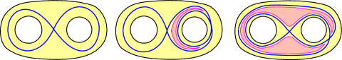
Figure 13. Three loops (in blue) filling a pair of pants. We highlighted the disks in the complement of the regular neighbourhood of the loop. The rightmost loop is double-filling while the two left ones are not.

Remark 8.5.

This notion does not depend on the choice of the loop $\gamma$ in a free-homotopy class. Indeed, we saw in the proof of 4.3 that two loops homotopic in $S$ can be obtained from one another by a sequence of third Reidemeister moves. Examining Figure 4, we can see that if a loop is double-filling according to our definition, then it remains so after a third Reidemeister move.

The double-filling hypothesis is a setting in which 8.1 is easy to prove.

Proposition 8.6.

For any $k\geq 0$, there exists a constant $c_{k}>0$ satisfying the following. For any local topological type $T=[S,\gamma]_{\mathrm{loc}}$, if $\chi_{S}=-1$ and $\gamma$ is a double-filling loop,

$$\int_{0}^{+\infty}\frac{|f_{k}^{T}(\ell)|}{(\ell+1)^{c_{k}}e^{\frac{\ell}{2}}}\,\mathrm{d}\ell\leq c_{k}.$$

In particular, $f_{k}^{T}$ is a Friedman–Ramanujan function in the weak sense, its degree and norm are $0$, and its constant and exponent are bounded by $c_{k}$.

The key element that allows to prove 8.6 is the following lemma.

Lemma 8.7.

Let $Y$ be a bordered hyperbolic surface, and $\gamma$ be a double-filling geodesic on $Y$. Then, $\ell_{Y}(\partial Y)\leq\ell_{Y}(\gamma)$.

This is an improvement of 4.4, which states that $\ell_{Y}(\partial Y)\leq 2\ell_{Y}(\gamma)$ whenever $\gamma$ fills $Y$. The double-filling hypothesis allows us to remove the factor $2$ in this length inequality, which comes from the fact that the regular neighbourhood of $\gamma$ has length approximately $2\ell_{Y}(\gamma)$. We first prove the lemma.

Proof of 8.7.

Let $\epsilon,\delta>0$, and $\mathcal{V}=\mathcal{V}_{\delta}(\gamma)$ be a $\delta$-regular neighbourhood of $\gamma$. By definition of a filling loop, each boundary component $b$ of $Y$ is homotopic to a non-contractible boundary components $b^{\mathcal{V}}$ of $\mathcal{V}$. By minimality of the length of the geodesic representative in a homotopy class, $\ell_{Y}(b)\leq\ell_{Y}(b^{\mathcal{V}})$ for all $b$. Thanks to the double-filling hypothesis, each $b^{\mathcal{V}}$ borders a disjoint simple portion of the loop $\gamma$, and therefore we can pick $\delta$ to be small enough so that

$$\ell_{Y}(\partial Y)\leq\sum_{b}\ell_{Y}(b^{\mathcal{V}})\leq\ell_{Y}(\gamma)+\epsilon.$$

This implies the claim taking $\epsilon\rightarrow 0$. ∎

We now proceed to the proof of 8.6.

Proof.

Let us first consider the case of a double-filling loop $\gamma$ on the pair of pants $P$, and $T:=[P,\gamma]_{\mathrm{loc}}$. Let $k\geq 0$ be an integer. By the proof of 5.14, see 5.23, for any admissible function $F$,

(8.1) $$\int_{0}^{+\infty}f_{k}^{T}(\ell)F(\ell)\,\mathrm{d}\ell=\frac{1}{m(T)}\int_{\mathbb{R}_{>0}^{3}}F(\mathcal{L}_{\gamma}(\ell_{1},\ell_{2},\ell_{3}))\,\psi_{k}^{P}(\ell_{1},\ell_{2},\ell_{3})\,\,\mathrm{d}\ell_{1}\,\mathrm{d}\ell_{2}\,\mathrm{d}\ell_{3}$$

where $\psi_{k}^{P}$ is the $k$-th term of the asymptotic expansion of the function $\phi_{g}^{P}$, expressed in 5.7, and $\mathcal{L}_{\gamma}:\mathbb{R}_{>0}^{3}\rightarrow\mathbb{R}$ is the function which, to the lengths of the three boundary components of $P$, associates the length of the geodesic $\gamma$. We take $c>0$ to be a parameter that we will adjust later. For any $L>0$, we apply (8.1) to the admissible function

$$\ell\mapsto\frac{\mathrm{sign}(f_{k}^{T}(\ell))}{(\ell+1)^{c}e^{\frac{\ell}{2}}}\,\mathds{1}_{[0,L]}(\ell)$$

and let $L\rightarrow+\infty$. We obtain that

(8.2) $$\int_{0}^{+\infty}\frac{|f_{k}^{T}(\ell)|}{(\ell+1)^{c}e^{\frac{\ell}{2}}}\,\mathrm{d}\ell\leq\int_{\mathbb{R}_{>0}^{3}}\frac{|\psi_{k}^{P}(\ell_{1},\ell_{2},\ell_{3})|}{(\mathcal{L}_{\gamma}(\ell_{1},\ell_{2},\ell_{3})+1)^{c}e^{\frac{\mathcal{L}_{\gamma}(\ell_{1},\ell_{2},\ell_{3})}{2}}}\,\mathrm{d}\ell_{1}\,\mathrm{d}\ell_{2}\,\mathrm{d}\ell_{3}.$$

We then use the double-filling hypothesis, and 8.7, to deduce that

(8.3) $$\int_{0}^{+\infty}\frac{|f_{k}^{T}(\ell)|}{(\ell+1)^{c}e^{\frac{\ell}{2}}}\,\mathrm{d}\ell\leq\int_{\mathbb{R}_{>0}^{3}}\frac{|\psi_{k}^{P}(\ell_{1},\ell_{2},\ell_{3})|}{(\ell_{1}+\ell_{2}+\ell_{3}+1)^{c}e^{\frac{\ell_{1}+\ell_{2}+\ell_{3}}{2}}}\,\mathrm{d}\ell_{1}\,\mathrm{d}\ell_{2}\,\mathrm{d}\ell_{3}.$$

5.21 allows us to write $\psi_{k}^{P}$ as a linear combination of certain kinds of functions, and it is easy to check that we can take a $c:=c_{k}$ such that (8.3) is $\mathcal{O}_{k}\left(1\right)$.

If now $\gamma$ is a double-filling loop on the once-holed torus $S_{1,1}$, then (8.1) is replaced by

$$\int_{0}^{+\infty}f_{k}^{T}(\ell)F(\ell)\,\mathrm{d}\ell=\int_{0}^{+\infty}\frac{1}{V_{1,1}(x)}\int_{\mathcal{T}_{1,1}(x)}\,F(\ell_{Y}(\gamma))\,\psi_{k}^{(1,1)}(x)\,\mathrm{d}\mathrm{Vol}_{1,1,x}^{\mathrm{\scriptsize{WP}}}(Y)\,\mathrm{d}x.$$

We shall prove that, for any $\ell,x>0$,

(8.4) $$\mathrm{Vol}_{1,1,x}^{\mathrm{\scriptsize{WP}}}(\{Y\in\mathcal{T}_{1,1}(x)\,:\,\ell_{Y}(\gamma)\leq\ell\})\leq 4\ell^{2}.$$

This allows to bound the integral over $\mathcal{T}_{1,1}(x)$, and then the rest of the proof is exactly identical to the pair of pants case above.

Let us equip $S_{1,1}$ with an arbitrary hyperbolic structure, and assume that $\gamma$ is the geodesic representative for this metric. We consider a parametrisation $\gamma:[0,1]\rightarrow S_{1,1}$. The loop $\gamma$ is filling and therefore not simple, and we can therefore define

$$t_{+}:=\inf\{t\geq 0\,:\,\exists s\in[0,t)\,:\,\gamma(s)=\gamma(t)\}$$

and $t_{-}<t_{+}$ so that $z:=\gamma(t_{-})=\gamma(t_{+})$. Then, the restriction $\gamma_{|[t_{-},t_{+}]}$ is a simple loop $\alpha$ on $S_{1,1}$ based at $z$.

The surface $S_{1,1}\setminus\alpha$ is a topological pair of pants $P$. We denote as $\alpha_{1}$ and $\alpha_{2}$ the two boundary components of $P$ corresponding to $\alpha$, so that the path $\gamma$ enters $P$ through $\alpha_{1}$ at the time $t_{+}$. We denote as $z_{1}$ and $z_{2}$ the copies of $z$ on $P$, following this numbering convention.

Let us consider a small enough $\epsilon>0$ such that $\mathcal{C}_{\epsilon}:=\{w\in P\,:\,0<\mathrm{dist}(w,\alpha_{2})<\epsilon\}$ is a cylinder. The loop $\gamma$ fills the surface $S_{1,1}$, and $\mathcal{C}_{\epsilon}$ is an annulus that is not homotopic to $\partial S_{1,1}$, and hence the set $\mathcal{C}_{\epsilon}$ cannot lie entirely in the complement of $\gamma$. We deduce that there exists a restriction $\beta_{0}$ of $\gamma$ (or $\gamma^{-1}$) going from a point of $\alpha_{2}$ to a point of $\partial P$ which cannot be homotoped to a path on $\alpha_{2}$. Because $\gamma$ does not intersect $\partial S_{1,1}$, there are two possibilities for the topology of $\beta_{0}$, represented in Figure 14.

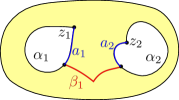
(a) The case (1).

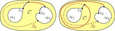
(b) Two possible scenarios in case (2).

Figure 14. Illustration of the proof of equation 8.4.

In both those cases, let us prove that can use pieces of $\gamma$ to create a simple closed loop $\beta$ on $S_{1,1}$ that intersects $\alpha$ exactly once.

1. If $\beta_{0}$ goes from $\alpha_{2}$ to $\alpha_{1}$, we extract a simple sub-path $\beta_{1}$ from it by iteratively removing the portion of $\beta_{0}$ restricted to $[u_{-},u_{+}]$ for any times $u_{-}<u_{+}$ such that $\beta_{0}(u_{-})=\beta_{0}(u_{+})$, until no intersections are left. We then take a sub-path $a_{2}$ of $\alpha_{2}$ from $z_{2}$ to the beginning of $\beta_{1}$, and a sub-path $a_{1}$ of $\alpha_{1}$ from the endpoint of $\beta_{1}$ to $z_{1}$. The concatenation $\beta:=a_{2}\mathord{\mathchoice{\,\vbox{\hbox{\scalebox{0.5}{$\displaystyle\bullet$}}}\,}{\,\vbox{\hbox{\scalebox{0.5}{$\textstyle\bullet$}}}\,}{\,\vbox{\hbox{\scalebox{0.5}{$\scriptstyle\bullet$}}}\,}{\,\vbox{\hbox{\scalebox{0.5}{$\scriptscriptstyle\bullet$}}}\,}}\beta_{1}\mathord{\mathchoice{\,\vbox{\hbox{\scalebox{0.5}{$\displaystyle\bullet$}}}\,}{\,\vbox{\hbox{\scalebox{0.5}{$\textstyle\bullet$}}}\,}{\,\vbox{\hbox{\scalebox{0.5}{$\scriptstyle\bullet$}}}\,}{\,\vbox{\hbox{\scalebox{0.5}{$\scriptscriptstyle\bullet$}}}\,}}a_{1}$ satisfies the hypotheses.

2. If $\beta_{0}$ goes from $\alpha_{2}$ to itself, then by construction it is not homotopic with fixed endpoints to a portion of $\alpha_{2}$. We use this information to find a topological cylinder $\mathcal{C}^{\prime}$ which has $\alpha_{1}$ as one boundary component, and portions of $\beta_{0}$ and perhaps $\alpha_{2}$ as the other. The path $\gamma$ enters $\mathcal{C}^{\prime}$ at time $t_{+}$, and cannot be homotoped to a sub-path of $\alpha_{1}$ (otherwise $S_{1,1}$ would contain a geodesic bigon). As a consequence, it has to escape the cylinder $\mathcal{C}^{\prime}$ by its other boundary component. We concatenate the portion of $\gamma$ from $t_{+}$ to its escape of $\mathcal{C}^{\prime}$, as well as portions of $\beta_{0}$, and finally a portion of $\alpha_{2}$ from the starting point of $\beta_{0}$ to $z_{2}$, to construct $\beta$.

Then, by construction,

$$\forall(x,Y)\in\mathcal{T}_{1,1}(x),\quad\begin{cases}\ell_{Y}(\alpha)\leq\ell_{Y}(\gamma)\\ \ell_{Y}(\beta)\leq 2\ell_{Y}(\gamma).\end{cases}$$

For $x>0$, we consider the Fenchel–Nielsen coordinates $(\ell_{1},\tau_{1})$ on $\mathcal{T}_{1,1}(x)$ so that $\ell_{1}$ is equal to $\ell_{Y}(\alpha)$, and the geodesics homotopic to $\alpha$ and $\beta$ are orthogonal when $\tau_{1}=0$. Then, an elementary computation yields

$$\cosh(\ell_{Y}(\gamma))\geq\cosh\left(\frac{\ell_{Y}(\beta)}{2}\right)=\cosh\left(\frac{\ell_{1}}{2}\right)\cosh\left(\frac{\tau_{1}}{2}\right)\geq\cosh\left(\frac{\tau_{1}}{2}\right)$$

and therefore, for any $\ell>0$,

$$\{(\ell_{1},\tau_{1})\in\mathbb{R}_{>0}\times\mathbb{R}\,:\,\ell_{Y}(\gamma)\leq\ell\}\subset[0,\ell]\times[-2\ell,2\ell]$$

which is enough to conclude to (8.4). ∎

8.2. Classification of filling loops that do not double-fill

Thanks to Sections 7 and 8.1, we now know that 8.1 holds for figure-eights and double-filling loops. We have seen, at the centre of Figure 13, an example of a loop filling a pair of pants which is neither a double-filling loop nor a figure-eight. We make the following definition to refer to this loop, and other similar examples.

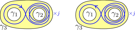
Figure 15. Two distinct one-sided figure eights with $j=3$ iterations.

Notation 8.8.

We call the local topological types represented in Figure 15 one-sided iterated eights, and refer to the integer $j$ as their number of iterations. For any $j\geq 2$, we denote as $\alpha_{j}$ the loop on the left-hand side of Figure 15.

We prove the following.

Proposition 8.9.

Let $S$ be a filling type of Euler characteristic $-1$. Then, for any loop $\gamma$ filling $S$, one and only of the two following occurs:

• either $\gamma$ is double-filling;

• or $S$ is a pair of pants, and $\gamma$ is a figure-eight or a one-sided iterated eight.

As a consequence, one-sided iterated eights are the only remaining case that we need to consider to prove Objective (FR) when $\chi_{S}=-1$. We shall do so in Section 8.3.

Proof.

First, let $S=P$ be a pair of pants, and $\gamma$ be a filling loop that is not double-filling. Let us prove that $\gamma$ is a figure-eight or a one-sided iterated eight.

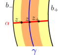
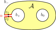
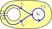
Figure 16. Illustration of the proof in the pair of pants case.

Let $\mathcal{V}$ be a regular neighbourhood of $\gamma$. By definition of double-filling loopss, there exists a simple portion of $\gamma$, denoted as $\beta$, such that $b_{\pm}^{\mathcal{V}}:=b_{\pm}^{\mathcal{V}}(\beta)$ are not contractible. They therefore are homotopic to two (non-necessarily distinct) boundary components $b_{\pm}$ of $P$. Let us pick a point $z$ on $\beta$, two neighbours $z_{\pm}$ of $z$ on $b_{\pm}^{\mathcal{V}}$, and a simple path $c_{0}$ going from $z_{+}$ to $z_{-}$ by crossing the regular neighbourhood $\mathcal{V}$ transversally, which only intersects $\gamma$ at the point $z$. For $\sigma\in\{+,-\}$, since $b_{\sigma}^{\mathcal{V}}$ and $b_{\sigma}$ delimit an annulus, there exists a simple path $c_{\sigma}$ entirely contained in this annulus going from $b_{\sigma}$ to $z_{\sigma}$. Then, we let $\alpha:=c_{+}\mathord{\mathchoice{\,\vbox{\hbox{\scalebox{0.5}{$\displaystyle\bullet$}}}\,}{\,\vbox{\hbox{\scalebox{0.5}{$\textstyle\bullet$}}}\,}{\,\vbox{\hbox{\scalebox{0.5}{$\scriptstyle\bullet$}}}\,}{\,\vbox{\hbox{\scalebox{0.5}{$\scriptscriptstyle\bullet$}}}\,}}c_{0}\mathord{\mathchoice{\,\vbox{\hbox{\scalebox{0.5}{$\displaystyle\bullet$}}}\,}{\,\vbox{\hbox{\scalebox{0.5}{$\textstyle\bullet$}}}\,}{\,\vbox{\hbox{\scalebox{0.5}{$\scriptstyle\bullet$}}}\,}{\,\vbox{\hbox{\scalebox{0.5}{$\scriptscriptstyle\bullet$}}}\,}}c_{-}^{-1}$, as represented in the left part of Figure 16. By construction, the path $\alpha$ is simple, and only intersects $\gamma$ once, at $z$. Let us cut the pair of pants $P$ along the simple path $\alpha$ going from $b_{+}$ to $b_{-}$.

If $b_{+}=b_{-}$, then the path $\alpha$ would separate the pair of pants $P$ it into two connected components, while it intersects $\gamma$ only once. This is impossible because the loop $\gamma$ is closed. As a consequence, $b_{+}\neq b_{-}$, and the result we obtain by cutting $P$ along $\alpha$ is therefore an annulus $\mathcal{A}$, as represented on the middle part of Figure 16.

The point $z$ corresponds to two marked points $z_{1}$ and $z_{2}$ on one boundary component of the annulus. Because $\gamma$ only intersects $\alpha$ once, at $z$, the path $\gamma$ corresponds to a path $\gamma^{\prime}$ on $\mathcal{A}$, going from $z_{1}$ to $z_{2}$. The fundamental group of an annulus is $\mathbb{Z}$, and therefore $\gamma^{\prime}$ is homotopic with fixed endpoint to $t_{1}\mathord{\mathchoice{\,\vbox{\hbox{\scalebox{0.5}{$\displaystyle\bullet$}}}\,}{\,\vbox{\hbox{\scalebox{0.5}{$\textstyle\bullet$}}}\,}{\,\vbox{\hbox{\scalebox{0.5}{$\scriptstyle\bullet$}}}\,}{\,\vbox{\hbox{\scalebox{0.5}{$\scriptscriptstyle\bullet$}}}\,}}b_{0}^{j}\mathord{\mathchoice{\,\vbox{\hbox{\scalebox{0.5}{$\displaystyle\bullet$}}}\,}{\,\vbox{\hbox{\scalebox{0.5}{$\textstyle\bullet$}}}\,}{\,\vbox{\hbox{\scalebox{0.5}{$\scriptstyle\bullet$}}}\,}{\,\vbox{\hbox{\scalebox{0.5}{$\scriptscriptstyle\bullet$}}}\,}}t_{2}^{-1}$ for a $j\in\mathbb{Z}$, where $b_{0}$ is the boundary component of $\mathcal{A}$ on which $z_{1}$ and $z_{2}$ do not lie, corresponding to the third boundary component of the pair of pants, and $t_{1}$, $t_{2}$ are paths from $z_{1}$, $z_{2}$ to a shared fixed point of $b_{0}$ (see the right-hand side of Figure 16). It follows that $\gamma$ is a figure-eight or a one-sided iterated eight.

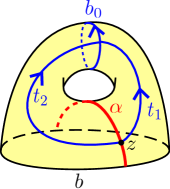
Figure 17. Illustration of the proof in the once-holed torus case.

Now, let us assume that $S$ is the once-holed torus $S_{1,1}$, and let $\gamma$ be a loop on $S_{1,1}$ that is not double-filling. We prove that $\gamma$ does not fill $S_{1,1}$. Indeed, let us construct $b_{-}$, $b_{+}$, $\alpha$ be as above. The once-holed torus $S_{1,1}$ only has one boundary component, i.e. $b_{-}=b_{+}=:b$. The surface $S_{1,1}\setminus\alpha$ has Euler characteristic $0$ and cannot be disconnected, since $\gamma$ is a closed loop intersecting $\alpha$ exactly once. As a consequence, it is an annulus. Let $z_{1}$ and $z_{2}$ denote the two copies of $z$, that lie on the two distinct boundary components of the annulus. The fundamental group of an annulus is $\mathbb{Z}$, so the path $\gamma$ on the annulus can be written as $t_{1}\mathord{\mathchoice{\,\vbox{\hbox{\scalebox{0.5}{$\displaystyle\bullet$}}}\,}{\,\vbox{\hbox{\scalebox{0.5}{$\textstyle\bullet$}}}\,}{\,\vbox{\hbox{\scalebox{0.5}{$\scriptstyle\bullet$}}}\,}{\,\vbox{\hbox{\scalebox{0.5}{$\scriptscriptstyle\bullet$}}}\,}}b_{0}^{j}\mathord{\mathchoice{\,\vbox{\hbox{\scalebox{0.5}{$\displaystyle\bullet$}}}\,}{\,\vbox{\hbox{\scalebox{0.5}{$\textstyle\bullet$}}}\,}{\,\vbox{\hbox{\scalebox{0.5}{$\scriptstyle\bullet$}}}\,}{\,\vbox{\hbox{\scalebox{0.5}{$\scriptscriptstyle\bullet$}}}\,}}t_{2}^{-1}$ for a $j\in\mathbb{Z}$, where $b_{0}$ is the core of the annulus and $t_{1}$, $t_{2}$ are two paths connecting $z_{1}$, $z_{2}$ to a shared point of $b_{0}$, as represented on Figure 17. This path admits a simple representative in the homotopy class with fixed endpoints, which corresponds to a simple loop on $S_{1,1}$ homotopic to $\gamma$. By minimality of the intersection number for the geodesic representation, this implies that $\gamma$ is simple. In particular, $\gamma$ does not fill $S_{1,1}$, which was our claim.

Because figure-eights and one-sided iterated eights are not double-filling, it is clear the two cases are mutually exclusive. ∎

8.3. Proof of the conjecture for one-sided iterated eights

Let us now proceed to the last step towards a proof of 8.1, which consists in proving it for any one-sided iterated eight. For any $j\geq 2$, there are exactly two distinct local types of one-sided iterated eights with $j$ iterations, represented on Figure 15. Because these two types only differ by orientation, we shall only study the local type $[P,\alpha_{j}]_{\mathrm{loc}}$. Let us prove the following statement.

Proposition 8.10.

For any $k\geq 0$, there exists a constant $c_{k}>0$ satisfying the following. For any $j\geq 2$, the function $f_{k}^{[P,\alpha_{j}]_{\mathrm{loc}}}$ is Friedman–Ramanujan, and its degree, norm and constant are smaller than $c_{k}$.

The proof is extremely similar to the case of the figure eight, done in detail in Section 7, and we shall therefore only sketch it. The first step we need to take is to compute the length-formula relating the length of the geodesic $\alpha_{j}$ to the three boundary lengths of the pair of pants, generalising equation 7.2 for $j\geq 1$. This leads to the following.

Lemma 8.11.

The expression for $(f_{k}^{[P,\alpha_{1}]_{\mathrm{loc}}})_{k\geq 0}$ from 7.3, true for the figure-eight, can be extended to any local topology $[P,\alpha_{j}]_{\mathrm{loc}}$ for $j\geq 2$ by replacing the length-function $\mathcal{L}$ in the level-set integrals by the new length-function $\mathcal{L}_{j}$ satisfying

(8.5) $$\cosh\left(\frac{\mathcal{L}_{j}(\ell_{1},\ell_{2},\ell_{3})}{2}\right)=\frac{\cosh\left(\frac{\ell_{1}}{2}\right)\sinh\left(\frac{(j+1)\ell_{2}}{2}\right)+\cosh\left(\frac{\ell_{3}}{2}\right)\sinh\left(\frac{j\ell_{2}}{2}\right)}{\sinh\left(\frac{\ell_{2}}{2}\right)}\cdot$$

The family of functions $(f_{i})_{i}$ and the coefficients that appear in this expansion does not depend on the parameter $j$.

Proof.

We simply follow the exact same steps as in Sections 7.1 to 7.6. The only difference here is that the expression of the length, (7.2) in the case of the figure eight, and (8.5) here. We prove that, for any $j\geq 2$,

(8.6) $$\cosh\left(\frac{\mathcal{L}_{j}(\ell_{1},\ell_{2},\ell_{3})}{2}\right)=2\cosh\left(\frac{\ell_{1}}{2}\right)\cosh\left(\frac{j\ell_{2}}{2}\right)+\cosh\left(\frac{\mathcal{L}_{j-1}(\ell_{3},\ell_{2},\ell_{1})}{2}\right).$$

We then obtain (8.5) by a straightforward induction.

The proof of equation 8.6 is a geometric argument, that uses the interpretation of the unit tangent bundle of the pair of pants $P$ as a quotient of $\mathrm{PSL}_{2}(\mathbb{R})$, and the formula $\cosh\left(\frac{\ell(\gamma)}{2}\right)=\frac{1}{2}|{\rm tr}(\gamma)|$ true for any hyperbolic element $\gamma$ of $\mathrm{PSL}_{2}(\mathbb{R})$. Because these tools only appear in this proof, we will not provide more introductory detail, and invite the reader to refer to [19] for more details.

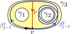
Figure 18. The geometric construction for the proof of equation 8.6.

The following construction is illustrated on Figure 18. Let $\beta_{j-1}$ denote the one-sided iterated eight obtained by going once around $\gamma_{3}$ and $j-1$ times around $\gamma_{2}$, which has length $\mathcal{L}_{j-1}(\ell_{3},\ell_{2},\ell_{1})$. Let $p$ denote the common perpendicular of $\beta_{j-1}$ with itself represented in Figure 18 – we shall also use the notation $p$ for its length. The endpoints of $p$ delimits two paths $\beta_{j-1}^{1}$ and $\beta_{j-1}^{2}$ obtained from $\beta_{j-1}$, of respective lengths denoted by $t_{1}$ and $t_{2}$. Then, the one-sided iterated eight $\alpha_{j}$, of length $\mathcal{L}_{j}(\ell_{1},\ell_{2},\ell_{3})$, is freely homotopic to $\beta_{j-1}^{1}\mathord{\mathchoice{\,\vbox{\hbox{\scalebox{0.5}{$\displaystyle\bullet$}}}\,}{\,\vbox{\hbox{\scalebox{0.5}{$\textstyle\bullet$}}}\,}{\,\vbox{\hbox{\scalebox{0.5}{$\scriptstyle\bullet$}}}\,}{\,\vbox{\hbox{\scalebox{0.5}{$\scriptscriptstyle\bullet$}}}\,}}p\mathord{\mathchoice{\,\vbox{\hbox{\scalebox{0.5}{$\displaystyle\bullet$}}}\,}{\,\vbox{\hbox{\scalebox{0.5}{$\textstyle\bullet$}}}\,}{\,\vbox{\hbox{\scalebox{0.5}{$\scriptstyle\bullet$}}}\,}{\,\vbox{\hbox{\scalebox{0.5}{$\scriptscriptstyle\bullet$}}}\,}}\beta_{j-1}^{2}\mathord{\mathchoice{\,\vbox{\hbox{\scalebox{0.5}{$\displaystyle\bullet$}}}\,}{\,\vbox{\hbox{\scalebox{0.5}{$\textstyle\bullet$}}}\,}{\,\vbox{\hbox{\scalebox{0.5}{$\scriptstyle\bullet$}}}\,}{\,\vbox{\hbox{\scalebox{0.5}{$\scriptscriptstyle\bullet$}}}\,}}p$. Transporting the vector $v$ represented on Figure 18 along this trajectory using elements of $\mathrm{SL}_{2}(\mathbb{R})$, we obtain that

(8.7) $$\cosh\left(\frac{\mathcal{L}_{j}(\ell_{1},\ell_{2},\ell_{3})}{2}\right)=\frac{1}{2}\,|{\rm tr}(a_{t_{1}}w_{p}a_{t_{2}}w_{-p})|$$

where

$$a_{t}:=\begin{pmatrix}e^{\frac{t}{2}}&0\\ 0&e^{-\frac{t}{2}}\end{pmatrix}\quad\text{and}\quad w_{p}:=\begin{pmatrix}\cosh\left(\frac{p}{2}\right)&\sinh\left(\frac{p}{2}\right)\\ \sinh\left(\frac{p}{2}\right)&\cosh\left(\frac{p}{2}\right)\end{pmatrix}$$

respectively correspond to moving the vector $v$ in a straight direction for a length $t$, or along the orthogonal geodesic in the right direction for the (algebraic) length $p$. We rewrite (8.7) as

(8.8) $$\cosh\left(\frac{\mathcal{L}_{j}(\ell_{1},\ell_{2},\ell_{3})}{2}\right)=\frac{1}{2}\,|{\rm tr}(A_{1}A_{2})|$$

where

(8.9) $$A_{1}:=a_{t_{1}}w_{p}R,\quad A_{2}:=R^{-1}a_{t_{2}}w_{-p},\quad\text{with}\quad R:=\begin{pmatrix}0&1\\ -1&0\end{pmatrix}.$$

In $\mathrm{SL}_{2}(\mathbb{R})$, we have that

(8.10) $${\rm tr}(A_{1}A_{2})={\rm tr}(A_{1})\,{\rm tr}(A_{2})+{\rm tr}(-A_{1}A_{2}^{-1}).$$

We observe by a direct computation that for $i=1,2$, ${\rm tr}(A_{i})=2\sinh\left(\frac{p}{2}\right)\sinh\left(\frac{t_{i}}{2}\right)>0$, and the path described by $A_{i}$ is freely homotopic to the closed geodesic $\gamma_{1}$ for $i=1$ and $\gamma_{2}^{j}$ for $i=2$. Hence,

(8.11) $${\rm tr}(A_{1})=2\cosh\left(\frac{\ell_{1}}{2}\right)\quad\text{and}\quad{\rm tr}(A_{2})=2\cosh\left(\frac{j\ell_{2}}{2}\right).$$

We use that $R^{-1}=-R$, $a_{t_{2}}^{-1}=a_{-t_{2}}$, $w_{p}^{-1}=w_{-p}$ and $R\,w_{p}a_{-t_{2}}\,R^{-1}=w_{-p}a_{t_{2}}$ to obtain

(8.12) $${\rm tr}(-A_{1}A_{2}^{-1})={\rm tr}(a_{t_{1}}w_{p}R\,w_{p}a_{-t_{2}}R^{-1})={\rm tr}(a_{t_{1}}a_{t_{2}})=2\cosh\left(\frac{\mathcal{L}_{j-1}(\ell_{3},\ell_{2},\ell_{1})}{2}\right).$$

The conclusion then follows from equations 8.7, 8.10, 8.11 and 8.12. ∎

In the case of the pair of pants, 7.4 allowed us to deal with a few elementary cases. We easily adapt it to this new setting, and prove the following.

Lemma 8.12.

For any $j\geq 2$, the integrals of the form (7.8) are always elements of $\mathcal{R}\subset\mathcal{F}$, and so is the integral (7.7) as soon as $p_{1}=0$ or $p_{3}=0$. The estimate on the remainders can be made uniformly in $j$.

Proof.

We only sketch the proof for $p_{1}=0$, because this case is actually new compared to before (in the case of the eight, we needed to assume $p_{1}=p_{2}=0$). The difference is the fact that, now,

$$\frac{\partial\ell_{3}}{\partial\ell}=\frac{\sinh\left(\frac{\ell_{2}}{2}\right)}{\sinh\left(\frac{j\ell_{2}}{2}\right)}\frac{\sinh\left(\frac{\ell}{2}\right)}{\sinh\left(\frac{\ell_{3}}{2}\right)}$$

and hence the integral we need to bound is

$$\sinh\left(\frac{\ell}{2}\right)\iint\left(\prod_{i=1}^{3}f_{i}(\ell_{i})\right)\sinh\left(\frac{\ell_{1}}{2}\right)\frac{\sinh^{2}\left(\frac{\ell_{2}}{2}\right)}{\sinh\left(\frac{j\ell_{2}}{2}\right)}\mathds{1}_{I(\ell_{1},\ell_{2})}(\ell)\,\mathrm{d}\ell_{1}\,\mathrm{d}\ell_{2}$$

which, if $p_{1}=0$, is clearly an element of $\mathcal{R}$, uniformly in $j$, because for any $j\geq 2$,

$$\frac{\sinh^{2}\left(\frac{\ell_{2}}{2}\right)}{\sinh\left(\frac{j\ell_{2}}{2}\right)}\leq\frac{\sinh^{2}\left(\frac{\ell_{2}}{2}\right)}{\sinh(\ell_{2})}=\mathcal{O}\left(1\right).$$

∎

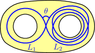
Figure 19. The coordinates for the one-sided iterated eight.

For the rest of the proof, we need to pick new variables, suited to the integration on the new level-set $\{(\ell_{1},\ell_{2},\ell_{3})\in\mathbb{R}_{>0}^{3}\,:\,\mathcal{L}_{j}(\ell_{1},\ell_{2},\ell_{3})=\ell\}$. We choose the natural adaptation of the case of the figure-eight, illustrated in Figure 19. More precisely, $L_{1}$ and $L_{2}$ denote the lengths of the two portions of $\alpha_{j}$ going around $\gamma_{1}$ (once) and $\gamma_{2}$ ($j$ times) respectively, so that $\ell_{P}(\alpha_{j})=L_{1}+L_{2}$. We once again let $u:=\cos^{2}\left(\frac{\theta}{2}\right)$, where $\theta$ is the angle represented on Figure 19. We then prove the following formula for the change of variables, generalising 7.6 for $j\geq 1$.

Lemma 8.13.

For any $j\geq 1$, any $\ell_{1},\ell_{2},\ell_{3}>0$,

$${}\begin{cases}&\cosh\left(\frac{\ell_{1}}{2}\right)=\sqrt{u}\,\cosh\left(\frac{L_{1}}{2}\right)\\ &\cosh\left(\frac{j\ell_{2}}{2}\right)=\sqrt{u}\,\cosh\left(\frac{L_{2}}{2}\right)\\ &\cosh\left(\frac{\ell_{3}}{2}\right)=a_{j}(\ell_{2})\left[(1-b_{j}(\ell_{2})\,u)\cosh\left(\frac{L_{1}+L_{2}}{2}\right)-b_{j}(\ell_{2})\,u\cosh\left(\frac{L_{1}-L_{2}}{2}\right)\right]\\ \end{cases}$$

where

$$a_{j}(\ell_{2}):=\frac{\sinh\left(\frac{\ell_{2}}{2}\right)}{\sinh\left(\frac{j\ell_{2}}{2}\right)}\quad\text{and}\quad b_{j}(\ell_{2}):=\frac{\sinh\left(\frac{(j+1)\ell_{2}}{2}\right)}{2\sinh\left(\frac{\ell_{2}}{2}\right)\cosh\left(\frac{j\ell_{2}}{2}\right)}\cdot$$

We then proceed to compute the expression of the Jacobian of the change of variables.

Lemma 8.14.

For any $j\geq 1$, the change of variable $(\ell_{1},\ell_{2},\ell_{3})\rightarrow(L_{1},L_{2},u)$ is a diffeomorphism from $\mathbb{R}_{>0}^{3}$ to an open set $\mathcal{E}_{j}$ of $\mathbb{R}_{>0}^{2}\times(0,1)$, and its Jacobian can be written as

$$\prod_{i=1}^{3}\sinh\left(\frac{\ell_{i}}{2}\right)\,\mathrm{d}\ell_{i}=-\sinh^{2}\left(\frac{L_{1}+L_{2}}{2}\right)\frac{\sinh^{2}\left(\frac{\ell_{2}}{2}\right)}{j\sinh^{2}\left(\frac{j\ell_{2}}{2}\right)}\,\mathrm{d}L_{1}\,\mathrm{d}L_{2}\,\mathrm{d}u.$$

Proof.

In order to compute the Jacobian, we shall use the expression of $\ell_{3}$ derived in 8.12:

$$\cosh\left(\frac{\ell_{3}}{2}\right) =\frac{\sinh\left(\frac{\ell_{2}}{2}\right)\cosh\left(\frac{L_{1}+L_{2}}{2}\right)-\cosh\left(\frac{\ell_{1}}{2}\right)\sinh\left(\frac{(j+1)\ell_{2}}{2}\right)}{\sinh\left(\frac{j\ell_{2}}{2}\right)}$$

$$=\mathrm{expr}(L_{1},L_{2},\ell_{1}(L_{1},L_{2},u),\ell_{2}(L_{1},L_{2},u)).$$

We observe that, by the chain rule, we can write the derivative of the previous equation according to $L_{1}$ as:

$$\frac{1}{2}\sinh\left(\frac{\ell_{3}}{2}\right)\frac{\partial\ell_{3}}{\partial L_{1}}=\frac{\sinh\left(\frac{\ell_{2}}{2}\right)}{2\sinh\left(\frac{j\ell_{2}}{2}\right)}\sinh\left(\frac{L_{1}+L_{2}}{2}\right)+\frac{\partial\ell_{1}}{\partial L_{1}}\partial_{3}\mathrm{expr}+\frac{\partial\ell_{2}}{\partial L_{1}}\partial_{4}\mathrm{expr}$$

and similar expressions are valid for the derivation with respect to $L_{2}$ and $u$. The advantage of these expressions is that it makes it clear that, when we compute the Jacobian, we can remove from the column of the variable $\ell_{3}$ the crossed terms in which the derivatives $\partial_{3}\mathrm{expr}$ and $\partial_{4}\mathrm{expr}$ appear, by subtracting multiples of the columns from the variables $\ell_{1}$ and $\ell_{2}$. We can therefore reduce ourselves to computing the determinant

$$\frac{\sinh\left(\frac{\ell_{2}}{2}\right)}{\sinh\left(\frac{\ell_{1}}{2}\right)j\sinh^{2}\left(\frac{j\ell_{2}}{2}\right)\sinh\left(\frac{\ell_{3}}{2}\right)}\begin{vmatrix}\sqrt{u}\sinh\left(\frac{L_{1}}{2}\right)&0&\sinh\left(\frac{L_{1}+L_{2}}{2}\right)\\ 0&\sqrt{u}\sinh\left(\frac{L_{2}}{2}\right)&\sinh\left(\frac{L_{1}+L_{2}}{2}\right)\\ \frac{1}{\sqrt{u}}\cosh\left(\frac{L_{1}}{2}\right)&\frac{1}{\sqrt{u}}\cosh\left(\frac{L_{2}}{2}\right)&0\end{vmatrix}$$

which yields the claimed expression. ∎

We will then be able to conclude using the following.

Proposition 8.15.

Let $(f_{i})_{1\leq i\leq 3}$ be functions satisfying (7.9). For any $j\geq 2$, the function

(8.13) $$\ell\mapsto\iint_{L_{1}+L_{2}=\ell}\left(\prod_{i=1}^{3}f_{i}(\ell_{i})\right)\frac{\sinh^{2}\left(\frac{\ell_{2}}{2}\right)}{j\sinh^{2}\left(\frac{j\ell_{2}}{2}\right)}\mathds{1}_{\mathcal{E}_{j}}(L_{1},L_{2},u)\frac{\,\mathrm{d}L_{1}\,\mathrm{d}L_{2}\,\mathrm{d}u}{\,\mathrm{d}\ell}$$

is equal to a polynomial function up to an error of size $\mathcal{O}\left((\ell+1)^{c}e^{-\ell/2}\right)$. Furthermore, the degree and coefficients of the polynomial, as well as $c$ and the implied constant, can be bounded uniformly in $j$.

The proof of 8.15 is a straightforward adaptation of the proof in the case of the figure-eight, thanks to the similarity of the formulas for the changes of variables. Actually, it is slightly more elementary thanks to the additional decay in $\ell_{2}$ in equation 8.13, which removes the polynomial behaviour of $\ell_{2}$ and hence allows to consider the dependency in $\ell_{2}$ as a “remainder term” directly.

9. The second-order term is not a Friedman–Ramanujan function

In this section, we shall prove the following result, the hyperbolic surface counterpart of Theorem 2.12 from [10] for random regular graphs.

Theorem 9.1.

The function $\ell\mapsto\ell f_{1}^{\mathrm{all}}(\ell)$ is not a Friedman–Ramanujan function in the weak sense.

We shall prove this by contradiction, grouping the following two observations.

• On the one hand, in Section 9.1, we prove that $\mathbb{P}_{g}^{\mathrm{\scriptsize{WP}}}\left(\lambda_{1}\leq a\right)$ is not very small as $g\rightarrow+\infty$ (for a fixed $a$). Indeed, we know that this probability goes to $0$ as soon as $a<\frac{3}{16}$ by [45, 21], but we show that it does so at the speed $1/g$ as $g\rightarrow+\infty$ only, and no faster.

• On the other hand, in Section 9.2, we show that, if $\ell\mapsto\ell f_{1}^{\mathrm{all}}(\ell)$ was Friedman–Ramanujan in the weak sense, then we would be able to prove that $\mathbb{P}_{g}^{\mathrm{\scriptsize{WP}}}\left(\lambda_{1}\leq a\right)$ goes to $0$ at a rate $1/g^{1+\delta}$ for a $\delta>0$.

9.1 could appear to be a contradiction, because we have shown that $f_{1}^{\mathrm{all}}$ is the sum of $f_{1}^{T}$ for all local types $T$ that are simple or filling a surface of Euler characteristic $-1$, and $\ell\mapsto\ell f_{1}^{T}(\ell)$ is Friedman–Ramanujan in the weak sense for all those types by 3.3 and 8.1. However, the class $\mathcal{F}_{w}$ is not stable by countable summation, so there is no contradiction.

The reader is invited to read this section thinking of the fact that the issue causing that $\ell f_{1}^{\mathrm{all}}(\ell)\notin\mathcal{F}_{w}$ is the possible existence of tangles, as introduced in [32, 21] for hyperbolic surfaces, and [10, 4] for random regular graphs. We shall see that tangles are small pairs of pants or once-holed tori, which contain “too many” closed geodesics, and cause the first non-zero eigenvalue $\lambda_{1}$ to be small.

9.1. Estimate of the probability of having a small eigenvalue

Let us prove the following result on the speed of convergence of $\mathbb{P}_{g}^{\mathrm{\scriptsize{WP}}}\left(\lambda_{1}\leq a\right)$ as $g\rightarrow+\infty$.

Theorem 9.2.

There exists $a_{0},c_{1},c_{2}>0$ such that, for any $a\leq a_{0}$, any large enough $g$,

(9.1) $$c_{1}\frac{a^{2}}{g}\leq\mathbb{P}_{g}^{\mathrm{\scriptsize{WP}}}\left(\lambda_{1}\leq a\right)\leq c_{2}\,\frac{a}{g}\cdot$$

The proof of the upper and lower bounds are different, and will be treated separately.

9.1.1. The lower bound

In order to prove the lower bound, we shall prove that, if a surface contains a once-holed torus with a short boundary, then it has a small eigenvalue.

Lemma 9.3.

Let $X$ be a compact hyperbolic surface of genus $g\geq 2$. We assume that $X$ contains an embedded once-holed torus $\mathcal{T}$ with geodesic boundary, and that $\ell_{X}(\partial\mathcal{T})\leq 1$. Then, $\lambda_{1}(X)\leq\ell_{X}(\partial\mathcal{T})$.

Proof.

The min-max principle allows to bound eigenvalues in terms of well-chosen Rayleigh quotients. A classic application, that can be found in [7, Theorem 8.2.1] for instance, states that, if $\phi_{1},\phi_{2}\in H^{1}(X)$ are $L^{2}$-orthogonal, then

(9.2) $$\lambda_{1}(X)\leq\max\left\{\frac{\int_{X}\|\operatorname{grad}\phi_{1}\|^{2}\,\mathrm{d}\mu}{\int_{X}|\phi_{1}|^{2}\,\mathrm{d}\mu},\frac{\int_{X}\|\operatorname{grad}\phi_{2}\|^{2}\,\mathrm{d}\mu}{\int_{X}|\phi_{2}|^{2}\,\mathrm{d}\mu}\right\},$$

where $\operatorname{grad}$ and $\,\mathrm{d}\mu$ are the gradient and volume form associated to the metric on $X$.

By the collar lemma [7, Theorem 4.1.1], the neighbourhood of width

$$\operatorname{arcsinh}\left(\sinh\left(\frac{\ell_{X}(\partial\mathcal{T})}{2}\right)^{-1}\right)$$

of $\partial T$ is isometric to a cylinder. As soon as $\ell_{X}(\partial\mathcal{T})\leq 1$, this width is larger than $\operatorname{arcsinh}(1/\sinh(1/2))>1$. We can therefore define two elements of $H^{1}(X)$ by

$$\phi_{1}(z):=\min(1,\mathrm{dist}(z,X\setminus\mathcal{T}))\quad\text{and}\quad\phi_{2}(z):=\min(1,\mathrm{dist}(z,\mathcal{T})).$$

These functions are $L^{2}$-orthogonal because they have disjoint support, and we can therefore apply the min-max principle to them. Let us estimate the Rayleigh quotients appearing in equation 9.2.

First, the norm of the gradient of $\phi_{1}$ is equal to $1$ on the set

$$\mathcal{T}^{-}:=\{z\in\mathcal{T}\,:\,\mathrm{dist}(z,X\setminus\mathcal{T})<1\},$$

and $0$ outside of it. Therefore,

$$\int_{X}\|\operatorname{grad}\phi_{1}\|^{2}\,\mathrm{d}\mu\leq\operatorname{Area}(\mathcal{T}^{-})=\int_{0}^{\ell_{X}(\partial\mathcal{T})}\int_{0}^{1}\cosh\rho\,\mathrm{d}\rho\,\mathrm{d}t=\sinh(1)\;\ell_{X}(\partial\mathcal{T})$$

where the area is computed using Fermi coordinates (see [7, Section 1.1]). We then observe that $\phi_{1}$ is identically equal to $1$ in $\mathcal{T}\setminus\mathcal{T}^{-}$, and hence

$$\int_{X}|\phi_{1}|^{2}\,\mathrm{d}\mu\geq\operatorname{Area}(\mathcal{T})-\operatorname{Area}(\mathcal{T}^{-})\geq 2\pi-\sinh(1)\,\ell_{X}(\partial\mathcal{T})\geq\pi$$

provided that $\ell_{X}(\partial\mathcal{T})\leq\pi/\sinh 1$, which is the case by hypothesis.

The function $\phi_{2}$ satisfies the same bounds. Therefore, equation 9.2 implies that $\lambda_{1}(X)\leq\sinh(1)\,\ell_{X}(\partial\mathcal{T})/\pi\leq\ell_{X}(\partial\mathcal{T})$, which is our claim. ∎

We then estimate the probability for a surface to contain a small once-holed torus.

Lemma 9.4.

There exists $a_{0},c_{1},c_{2}>0$ such that, for any $a\leq a_{0}$, any large enough $g$,

(9.3) $$c_{1}\,\frac{a^{2}}{g}\leq\mathbb{P}_{g}^{\mathrm{\scriptsize{WP}}}\left(\exists\text{ once-holed torus }\mathcal{T}\subset X\,:\,\ell_{X}(\partial\mathcal{T})\leq a\right)\leq c_{2}\,\frac{a^{2}}{g}\cdot$$

The proof of the lower bound of 9.2 then directly follows, because for any small enough $a$ and large enough $g$,

$$\mathbb{P}_{g}^{\mathrm{\scriptsize{WP}}}\left(\lambda_{1}\leq a\right)\underset{\text{Lemma }\ref{lem:minmax}}{\geq}\mathbb{P}_{g}^{\mathrm{\scriptsize{WP}}}\left(\exists\text{ once-holed torus }\mathcal{T}\subset X\,:\ell_{X}(\partial\mathcal{T})\leq a\right)\underset{\text{Lemma }\ref{lem:once_holed}}{\geq}c_{1}\frac{a^{2}}{g}\cdot$$

We actually only need the lower bound part of 9.4 to conclude to the lower bound of 9.2, but it is the hard part of the statement.

The proof of 9.4 is inspired by Mirzakhani’s proof of the fact that

$$c_{1}\,a^{2}\leq\mathbb{P}_{g}^{\mathrm{\scriptsize{WP}}}\left(\exists\text{ closed geodesic }\gamma\text{ on }X\,:\,\ell_{X}(\gamma)\leq a\right)\leq c_{2}\,a^{2},$$

done in [27, Theorem 4.2]. We adapt it to count small once-holed tori rather than small closed geodesics.

Proof.

For $a>0$, let $\mathcal{N}_{a}^{\mathcal{T}}(X)$ denote the number of once-holed tori $\mathcal{T}$ with geodesic boundary embedded in $X$ such that $\ell_{X}(\partial\mathcal{T})\leq a$. Let us estimate $\mathbb{P}_{g}^{\mathrm{\scriptsize{WP}}}\left(\mathcal{N}_{a}^{\mathcal{T}}\geq 1\right)$.

Step 1: expectation estimate. It is easy to compute the expectation of the random variable $\mathcal{N}_{a}^{\mathcal{T}}$, because it is a geometric function, and we can therefore apply Mirzakhani’s integration formula:

$$\mathbb{E}_{g}^{\mathrm{\scriptsize{WP}}}\big{[}\mathcal{N}_{a}^{\mathcal{T}}\big{]}=\frac{1}{V_{g}}\int_{0}^{a}V_{1,1}(x)\,V_{g-1,1}(x)\,x\,\mathrm{d}x.$$

We know by [33] that $V_{1,1}(x)=\pi^{2}/12+x^{2}/48$. We then replace $V_{g-1,1}(x)$ by its first-order approximation, see (2.8), and obtain that

(9.4) $$\mathbb{E}_{g}^{\mathrm{\scriptsize{WP}}}\big{[}\mathcal{N}_{a}^{\mathcal{T}}\big{]}=\frac{V_{g-1,1}}{V_{g}}\int_{0}^{a}\left(\frac{\pi^{2}}{6}+\frac{x^{2}}{12}\right)\sinh\left(\frac{x}{2}\right)\,\mathrm{d}x+\mathcal{O}\left(\frac{V_{g-1,1}}{gV_{g}}\int_{0}^{a}(1+x)^{4}\,e^{\frac{x}{2}}\,\mathrm{d}x\right).$$

Since $1/2<\pi^{2}/12<1$, we can take $a_{0}$ to be small enough so that

(9.5) $$\forall x\in[0,a_{0}],\quad\frac{x}{2}\leq\left(\frac{\pi^{2}}{6}+\frac{x^{2}}{12}\right)\sinh\left(\frac{x}{2}\right)\leq x.$$

By equations (2.4) and (2.5), the volume ratio is

(9.6) $$\frac{V_{g-1,1}}{V_{g}}=\frac{V_{g-1,1}}{V_{g-1,2}}\,\frac{V_{g-1,2}}{V_{g}}=\frac{1}{8\pi^{2}g}+\mathcal{O}\left(\frac{1}{g^{2}}\right).$$

Equations (9.4) to (9.6) together imply the existence of constants $c_{1},c_{2}$ (depending on $a_{0}$) such that, for any $a<a_{0}$,

(9.7) $$c_{1}\frac{a^{2}}{g}\leq\mathbb{E}_{g}^{\mathrm{\scriptsize{WP}}}\big{[}\mathcal{N}_{a}^{\mathcal{T}}\big{]}\leq c_{2}\frac{a^{2}}{g}\cdot$$

Step 2: from the expectation to the probability. By Markov’s inequality, we can directly obtain the upper bound part of the claim:

$$\mathbb{P}_{g}^{\mathrm{\scriptsize{WP}}}\left(\mathcal{N}_{a}^{\mathcal{T}}\geq 1\right)\leq\mathbb{E}_{g}^{\mathrm{\scriptsize{WP}}}\big{[}\mathcal{N}_{a}^{\mathcal{T}}\big{]}\leq c_{2}\,\frac{a^{2}}{g}\cdot$$

The other side of the inequality is harder to obtain because there is no lower bound on $\mathbb{P}(N\geq 1)$ in term of $\mathbb{E}[N]$ in general. We shall express the expectation of $\mathcal{N}_{a}^{\mathcal{T}}$ as

(9.8) $$\mathbb{E}_{g}^{\mathrm{\scriptsize{WP}}}\big{[}\mathcal{N}_{a}^{\mathcal{T}}\big{]}=\sum_{k=1}^{+\infty}\mathbb{P}_{g}^{\mathrm{\scriptsize{WP}}}\left(\mathcal{N}_{a}^{\mathcal{T}}\geq k\right)=\mathbb{P}_{g}^{\mathrm{\scriptsize{WP}}}\left(\mathcal{N}_{a}^{\mathcal{T}}\geq 1\right)+\sum_{k=2}^{+\infty}\mathbb{P}_{g}^{\mathrm{\scriptsize{WP}}}\left(\mathcal{N}_{a}^{\mathcal{T}}\geq k\right).$$

Thanks to this expression, we observe that in order to prove that $\mathbb{P}_{g}^{\mathrm{\scriptsize{WP}}}\left(\mathcal{N}_{a}^{\mathcal{T}}\geq 1\right)$ is bounded below by $c_{1}^{\prime}a^{2}/g$, it is sufficient to prove that $\sum_{k=2}^{+\infty}\mathbb{P}_{g}^{\mathrm{\scriptsize{WP}}}\left(\mathcal{N}_{a}^{\mathcal{T}}\geq k\right)$ is negligible compared to $a^{2}/g$. This reduces the problem to studying the probability for a typical surface to contain multiple small once-hole tori.

Let $X$ be a compact hyperbolic surface of genus $g$. Let us describe the topology of families of embedded once-holed tori in the surface $X$. In order to make the discussion simpler, let us assume that $a_{0}\leq 2\operatorname{arcsinh}1$. Then, by the collar lemma [7, Theorem 4.1.6], all closed geodesics shorter than $a_{0}$ on $X$ are pairwise disjoint. As a consequence, if $X$ contains $k$ once-holed tori $\mathcal{T}_{1},\ldots,\mathcal{T}_{k}$ of boundary lengths $\leq a\leq a_{0}$, then they are all disjoint (here, we assume that $g>2$, so that no two embedded once-holed tori can share a boundary component). Let $C$ denote the surface obtained by removing all of these once-holed tori from $X$. Since the once-holed tori only have one boundary component and the surface $X$ is connected, $C$ is also connected. It has $k$ boundary components (corresponding to the $k$ once-holed tori). By additivity of the Euler characteristic, the genus of $C$ is $g-k$, and in particular $k\leq g$.

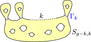
Figure 20. The multi-curve $\Gamma_{k}$ that separates $k$ once-holed tori off a surface of genus $g$.

Therefore, for any $1\leq k\leq g$, there is exactly one topological type of family of $k$ once-holed tori in a surface of genus $g$ (and none for $k>g$). Let us take a multi-curve $\Gamma_{k}$ of this topological type on the base surface $S_{g}$, as represented in Figure 20. We consider the function

$$F_{a,k}:\begin{cases}\mathbb{R}_{\geq 0}^{k}&\rightarrow\mathbb{R}\\ (x_{1},\ldots,x_{k})&\displaystyle\mapsto\frac{1}{k!}\prod_{i=1}^{k}\mathds{1}_{[0,a]}(x_{i}).\end{cases}$$

Then, the geometric function $X\mapsto F_{a,k}^{\Gamma_{k}}(X)$ defined by (2.2) exactly counts the number of undordered families of $k$ embedded once-holed tori with boundary length $\leq a$. Hence,

$$\mathbb{P}_{g}^{\mathrm{\scriptsize{WP}}}\left(\mathcal{N}_{a}^{\mathcal{T}}\geq k\right)=\mathbb{P}_{g}^{\mathrm{\scriptsize{WP}}}\left(F_{a,k}^{\Gamma_{k}}\geq 1\right)\leq\mathbb{E}_{g}^{\mathrm{\scriptsize{WP}}}\Big{[}F_{a,k}^{\Gamma_{k}}\Big{]}$$

by Markov’s inequality. We compute the expectation of this geometric function using Mirzakhani’s integration formula:

(9.9) $$\mathbb{P}_{g}^{\mathrm{\scriptsize{WP}}}\left(\mathcal{N}_{a}^{\mathcal{T}}\geq k\right)\leq\frac{1}{k!}\frac{1}{V_{g}}\int_{[0,a]^{k}}V_{g-k,k}(x_{1},\ldots,x_{k})\prod_{i=1}^{k}V_{1,1}(x_{i})\,x_{i}\,\mathrm{d}x_{i}.$$

We use once again [33] to express the volume $V_{1,1}(x_{i})$. By equation 2.7 and [27, Lemma 3.2], there exists a constant $C>0$ independent of $k$ such that

$$\frac{V_{g-k,k}(x_{1},\ldots,x_{k})}{V_{g}}\leq\frac{C^{k}}{g^{k}}\exp\left(\frac{x_{1}+\ldots+x_{k}}{2}\right).$$

Then, equation 9.9 becomes

$$\mathbb{P}_{g}^{\mathrm{\scriptsize{WP}}}\left(\mathcal{N}_{a}^{\mathcal{T}}\geq k\right)=\mathcal{O}\left(\frac{C^{k}}{k!}\frac{1}{g^{k}}\left[\int_{0}^{a}\left(\frac{\pi^{2}}{12}+\frac{x^{2}}{48}\right)x\exp\left(\frac{x}{2}\right)\,\mathrm{d}x\right]^{k}\right)=\mathcal{O}\left(\frac{C^{k}}{k!}\frac{a^{2k}}{g^{k}}\right),$$

provided we picked $a_{0}$ to be small enough. We deduce from the previous inequality that

(9.10) $$\sum_{k=2}^{+\infty}\mathbb{P}_{g}^{\mathrm{\scriptsize{WP}}}\left(\mathcal{N}_{a}^{\mathcal{T}}\geq k\right)=\mathcal{O}\left(\sum_{k=2}^{+\infty}\frac{C^{k}}{k!}\frac{a^{2k}}{g^{k}}\right)=\mathcal{O}\left(\frac{a^{4}}{g^{2}}\,e^{\frac{Ca^{2}}{g}}\right)=\mathcal{O}\left(\frac{a^{4}}{g^{2}}\right)$$

which is negligible compared to $\frac{a^{2}}{g}$ for small enough $a$ and large enough $g$. Our claim then follows directly by putting together equations 9.7, 9.8 and 9.10. ∎

9.1.2. The upper bound

Let us now prove the upper bound part of 9.2. It cannot be done the same way as the lower bound. Indeed, we have used the fact that, by the min-max principle, the presence of a small once-holed torus implies the presence of a small eigenvalue. But the converse is not true, and the existence of a small eigenvalue does not imply that the surface contains a small once-holed torus. We shall therefore rather rely on another geometric quantity, the Cheeger constant $h(X)$, defined by

$$h(X):=\inf_{A\sqcup B=X}\left\{\frac{\ell(\partial A)}{\min(\operatorname{Area}(A),\operatorname{Area}(B))}\right\}$$

where the infimum is taken over all partitions $A\sqcup B$ of $X$ into two smooth connected components. Cheeger’s inequality [9] states that

(9.11) $$\lambda_{1}(X)\geq\frac{h(X)^{2}}{4}$$

and in particular, if $\lambda_{1}(X)$ is small, then $h(X)$ is too (the converse is also true by Buser’s inequality [6]).

The Cheeger constant $h(X)$ is a priori difficult to estimate for random Weil–Petersson surfaces, because it does not depend only on geometric functions. In [27, Section 4.5], Mirzakhani defined a modified Cheeger constant $H(X)$. It is defined the same way as $h(X)$ is, except the infimum ranges over all partitions $A\sqcup B$ of $X$ into two connected components such that $\partial A$ is a union of disjoint simple geodesics. Mirzakhani proved in [27, Proposition 4.6] that the two Cheeger constants satisfy the inequality

(9.12) $$\frac{H(X)}{1+H(X)}\leq h(X)\leq H(X)$$

where the upper bound is trivial. In particular, $h(X)$ is small if and only if $H(X)$ is.

We shall use the following probabilistic estimate on $H(X)$.

Lemma 9.5.

There exists $c,a_{0}>0$ such that, for any $a\leq a_{0}$ and any large enough $g$,

(9.13) $$\mathbb{P}_{g}^{\mathrm{\scriptsize{WP}}}\left(H(X)\leq a\right)\leq c\frac{a^{2}}{g}\cdot$$

The upper bound of 9.2 then follows, because for any small enough $a$ and large enough $g$,

$$\mathbb{P}_{g}^{\mathrm{\scriptsize{WP}}}\left(\lambda_{1}\leq a\right)\underset{\eqref{eq:cheeger_ineq}}{\leq}\mathbb{P}_{g}^{\mathrm{\scriptsize{WP}}}\left(h(X)\leq 2\sqrt{a}\right)\underset{\eqref{eq:mirz_cheeger}}{\leq}\mathbb{P}_{g}^{\mathrm{\scriptsize{WP}}}\left(H(X)\leq\frac{2\sqrt{a}}{1-2\sqrt{a}}\right)\underset{\eqref{eq:mirz_prob_cheeger}}{\leq}c_{2}\,\frac{a}{g}\cdot$$

9.5 comes as a consequence of the proof of [27, Theorem 4.8], also it is not stated as such. For the sake of self-containment, we repeat the argument here.

Proof.

For a surface $X$, let $\Gamma$ be a multi-curve candidate to realising the modified Cheeger constant $H(X)$. The topological type of $\Gamma$ is entirely determined by its number of components, denoted by $k$, and the genera $g_{1}$ and $g_{2}$ of the two connected components of $X\setminus\Gamma$. We pick the numbering so that $g_{1}\leq g_{2}$, and note that by additivity of the Euler characteristic, we always have $g_{1}+g_{2}+k=g+1$. For such a $g_{1}$ and $k$, we fix one multi-curve $\Gamma_{g_{1},k}$ on the base surface $S_{g}$ of this topology. Then,

(9.14) $$\mathbb{P}_{g}^{\mathrm{\scriptsize{WP}}}\left(H(X)\leq a\right)\leq\sum_{\begin{subarray}{c}g_{1}+g_{2}+k=g+1\\ 0\leq g_{1}\leq g_{2}\\ g_{1}+k>1\end{subarray}}\mathbb{P}_{g}^{\mathrm{\scriptsize{WP}}}\left(H_{g_{1},k}(X)\leq a\right),$$

where for any $g_{1},k$, the function $H_{g_{1},k}$ is defined by

(9.15) $$H_{g_{1},k}(X):=\frac{\min\left\{\ell_{X}(\Gamma)\,:\,\Gamma\in\mathrm{Orb}_{g}(\Gamma_{g_{1},k})\right\}}{2\pi(2g_{1}-2+k)}\cdot$$

By Markov’s inequality and Mirzakhani’s integration formula,

$$\mathbb{P}_{g}^{\mathrm{\scriptsize{WP}}}\left(H_{g_{1},k}(X)\leq a\right)\leq\frac{1}{V_{g}}\frac{1}{k!}\int_{\mathbb{R}_{>0}^{k}}V_{g_{1},k}(\mathbf{x})V_{g_{2},k}(\mathbf{x})\,\mathds{1}_{[0,L_{g_{1},k}(a)]}(x_{1}+\ldots+x_{k})\,\prod_{i=1}^{k}x_{i}\,\mathrm{d}x_{i}$$

for $L_{g_{1},k}(a):=2\pi a(2g_{1}-2+k)$. This can be bounded using equation 2.7 and the fact that

$$\forall L>0,\quad\int_{\mathbb{R}_{>0}^{k}}\mathds{1}_{[0,L]}(x_{1}+\ldots+x_{k})\prod_{i=1}^{k}x_{i}\,\mathrm{d}x_{i}\leq\frac{L^{2k}}{(2k)!}$$

and we obtain that

$$\mathbb{P}_{g}^{\mathrm{\scriptsize{WP}}}\left(H_{g_{1},k}(X)\leq a\right)\leq\frac{1}{V_{g}}\frac{L_{g_{1},k}(a)^{2k}e^{L_{g_{1},k}(a)}}{k!(2k)!}V_{g_{1},k}V_{g_{2},k}\cdot$$

In order to sum over all values of $k$, we now set $g_{i}^{\prime}=g_{i}+\lfloor\frac{k}{2}\rfloor$ and $n=k-2\lfloor\frac{k}{2}\rfloor\in\{0,1\}$. We also assume that $2\pi a_{0}\leq 1$. By [27, Lemma 3.2 (3)], $V_{g_{1},k}V_{g_{2},k}=\mathcal{O}\left(V_{g_{1}^{\prime},n}V_{g_{2}^{\prime},n}\right)$ and hence

$$\mathbb{P}_{g}^{\mathrm{\scriptsize{WP}}}\left(H_{g_{1},k}(X)\leq a\right)=\mathcal{O}\left(\frac{a^{2}}{V_{g}}\frac{(2g_{1}^{\prime}-2+n)^{2k}}{k!(2k)!}\,e^{2\pi a(2g_{1}^{\prime}-2+n)}\,V_{g_{1}^{\prime},n}V_{g_{2}^{\prime},n}\right)$$

with a constant independent of $k$ (note that we have kept a term $a^{2}$ in this estimate, granted by the fact that $k\geq 1$; this is the only difference with Mirzakhani’s proof). We have that, for any $x$,

$$\sum_{k=1}^{+\infty}\frac{x^{2k}}{k!(2k)!}=\mathcal{O}\left(\exp\left(\frac{3}{2}x^{\frac{2}{3}}\right)\right)$$

and hence, equation 9.14 yields

$$\mathbb{P}_{g}^{\mathrm{\scriptsize{WP}}}\left(H(X)\leq a\right)=\mathcal{O}\left(\frac{a^{2}}{V_{g}}\sum_{n=0}^{1}\sum_{\begin{subarray}{c}g_{1}^{\prime}\leq g_{2}^{\prime}\\ g^{\prime}_{1}+g^{\prime}_{2}=g+1-n\end{subarray}}e^{2\pi a(2g_{1}^{\prime}-2+n)+\frac{3}{2}(2g_{1}^{\prime}-2+n)^{\frac{2}{3}}}V_{g_{1}^{\prime},n}V_{g_{2}^{\prime},n}\right).$$

In [27, Corollary 3.7], Mirzakhani proved that, provided that $4\pi a_{0}<2\log(2)$, the sum over all values of $g_{1}^{\prime},g_{2}^{\prime}$ is $\mathcal{O}\left(V_{g}/g\right)$ for $n=0$ and $n=1$, which allows us to conclude. ∎

9.2. Contradiction if $\ell f_{1}^{\mathrm{all}}(\ell)$ is Friedman–Ramanujan

Let us now prove that, if the function $\ell\mapsto\ell f_{1}^{\mathrm{all}}(\ell)$ was Friedman–Ramanujan in the weak sense, then we would be able to prove spectral estimates that are too good to be true.

Lemma 9.6.

If $\ell\mapsto\ell f_{1}^{\mathrm{all}}(\ell)$ is Friedman–Ramanujan in the weak sense, then for any small enough $\delta>0$, any large enough $g$,

$$\mathbb{P}_{g}^{\mathrm{\scriptsize{WP}}}\left(\delta\leq\lambda_{1}\leq\frac{5}{72}\right)=\mathcal{O}_{\delta}\left(g^{-\frac{5}{4}}\right).$$

Proof.

Let us assume that $\ell\mapsto\ell f_{1}^{\mathrm{all}}(\ell)$ is a Friedman–Ramanujan function in the weak sense, and denote as $d$ its degree. We shall use the trace method developed in Section 3.4, with the parameters:

$$A=6,\quad\alpha=\frac{5}{12}<\frac{1}{2},\quad\epsilon=\frac{1}{144},\quad m=\max(d,0)+1.$$

We observe that $1/4-\alpha^{2}-\epsilon=5/72$ and $(\alpha+\epsilon)A>\alpha A=5/2$, and therefore 3.14 implies that

(9.16) $$\mathbb{P}_{g}^{\mathrm{\scriptsize{WP}}}\left(\delta\leq\lambda_{1}\leq\frac{5}{72}\right)=\mathcal{O}_{\delta}\left(g^{-\frac{5}{2}}\left\langle\ell e^{-\frac{\ell}{2}}\,\mathcal{D}^{m}h_{L}(\ell)\right\rangle_{g}^{{\mathrm{all}}}+g^{-\frac{3}{2}}\right)\cdot$$

We then use the density-writing of the average $\langle\cdot\rangle_{g}^{{\mathrm{all}}}$, to write

(9.17) $$\left\langle\ell\,e^{-\frac{\ell}{2}}\,\mathcal{D}^{m}h_{L}(\ell)\right\rangle_{g}^{{\mathrm{all}}}=\int_{0}^{+\infty}e^{-\frac{\ell}{2}}\,\mathcal{D}^{m}h_{L}(\ell)\frac{\ell V_{g}^{\mathrm{all}}(\ell)}{V_{g}}\mathds{1}_{[0,L]}(\ell)\,\mathrm{d}\ell$$

because $\mathcal{D}^{m}h_{L}$ is identically equal to zero outside of $[0,L]$. By our asymptotic expansion result for the sum over all geodesics, 6.3, at the second order ($K=1$), using a fixed $\epsilon^{\prime}<1/24$,

(9.18) $$\frac{\ell\,V_{g}^{\mathrm{all}}(\ell)}{V_{g}}\mathds{1}_{[0,L]}(\ell)=F_{g,1}^{\mathrm{all}}(\ell)+\mathcal{O}^{w}\left(\frac{\ell\,e^{(1+\epsilon^{\prime})\ell}}{g^{2}}\right)=F_{g,1}^{\mathrm{all}}(\ell)+\mathcal{O}^{w}\left(\frac{e^{\frac{25\ell}{24}}}{g^{2}}\right)$$

for $F_{g,1}^{\mathrm{all}}(\ell):=\ell f_{0}^{\mathrm{all}}(\ell)+g^{-1}\ell f_{1}^{\mathrm{all}}(\ell)$. When we inject (9.18) into (9.17), we obtain

(9.19) $$\left\langle\ell\,e^{-\frac{\ell}{2}}\,\mathcal{D}^{m}h_{L}(\ell)\right\rangle_{g}^{{\mathrm{all}}}=\int_{0}^{L}F_{g,1}^{\mathrm{all}}(\ell)\,e^{-\frac{\ell}{2}}\,\mathcal{D}^{m}h_{L}(\ell)\,\mathrm{d}\ell+\mathcal{O}\left(g^{\frac{5}{4}}\right)$$

because the remainder is

$$\mathcal{O}\left(\frac{\|\mathcal{D}^{m}h_{L}\|_{\infty}}{g^{2}}e^{\frac{25L}{24}-\frac{L}{2}}\right)=\mathcal{O}\left(\frac{e^{\frac{13L}{24}}}{g^{2}}\right)=\mathcal{O}\left(g^{\frac{13}{4}-2}\right)=\mathcal{O}\left(g^{\frac{5}{4}}\right).$$

We know that $\ell f_{0}^{\mathrm{all}}(\ell)=4\sinh^{2}\left(\frac{\ell}{2}\right)$ is a Friedman–Ramanujan function, and therefore our hypothesis implies that $F_{g,1}^{\mathrm{all}}$ is an element of $\mathcal{F}_{w}$. Its degree is at most $\max(d,0)$, its norm, exponent and constant can be bounded by a uniform constant $c$. As a consequence, by 3.16, for $m=\max(d,0)+1$,

$$\int_{0}^{L}F_{g,1}^{\mathrm{all}}(\ell)\,e^{-\frac{\ell}{2}}\,\mathcal{D}^{m}h_{L}(\ell)\,\mathrm{d}\ell=\mathcal{O}\left(L^{c}\right).$$

Together with equation 9.19, this implies that $\left\langle\ell\,e^{-\frac{\ell}{2}}\,\mathcal{D}^{m}h_{L}(\ell)\right\rangle_{g}^{{\mathrm{all}}}=\mathcal{O}\left(g^{\frac{5}{4}}\right)$. The conclusion then follows directly from equation 9.16. ∎

We conclude with the proof of 9.1.

Proof.

Let us assume by contradiction that $\ell\mapsto\ell f_{1}^{\mathrm{all}}(\ell)$ is a Friedman–Ramanujan function in the weak sense. By 9.6, for any small enough $\delta>0$,

$$\mathbb{P}_{g}^{\mathrm{\scriptsize{WP}}}\left(\delta\leq\lambda_{1}\leq\frac{5}{72}\right)\leq C_{\delta}g^{-\frac{5}{4}}.$$

This is in particular also true if we replace $5/72$ by $a:=\min(a_{0},5/72)$, where $a_{0}$ is the constant from 9.2. Applying this result yields

$$\mathbb{P}_{g}^{\mathrm{\scriptsize{WP}}}\left(\delta\leq\lambda_{1}\leq a\right)=\mathbb{P}_{g}^{\mathrm{\scriptsize{WP}}}\left(\lambda_{1}\leq a\right)-\mathbb{P}_{g}^{\mathrm{\scriptsize{WP}}}\left(\lambda_{1}<\delta\right)\geq c_{1}\frac{a^{2}}{g}-c_{2}\frac{\delta}{g}$$

for some constants $c_{1},c_{2}>0$. We take $\delta$ to be a fixed number smaller than $a^{2}c_{1}/(2c_{2})$. Then, we obtain that, for any large enough $g$,

$$c_{1}\frac{a^{2}}{2}\leq g\,\mathbb{P}_{g}^{\mathrm{\scriptsize{WP}}}\left(\delta\leq\lambda_{1}\leq a\right)\leq C_{\delta}g^{-\frac{1}{4}}$$

which is a contradiction as $g\rightarrow+\infty$. ∎

10. Typical surfaces have a spectral gap at least $\frac{2}{9}-\epsilon$

We conclude this article by proving the following result, which improves the best known spectral gap result for random compact hyperbolic surfaces of high genus sampled using the Weil–Petersson probability measure.

Theorem 10.1.

For any $\epsilon>0$,

$$\mathbb{P}_{g}^{\mathrm{\scriptsize{WP}}}\left(\lambda_{1}\geq\frac{2}{9}-\epsilon\right)\underset{g\rightarrow+\infty}{\longrightarrow}1.$$

The main challenge in this proof is that we need to make a probabilistic hypothesis in order to remove tangles, which requires to adapt the methods developed in this article to more general averages that include an indicator function. This work is done in Sections 10.1 to 10.3. We then conclude to the proof of 10.1 in Section 10.4.

10.1. The tangle-free hypothesis and its geometric implications

In order to overcome the difficulties exposed in Section 9, we need to make a probabilistic hypothesis, which allows us to remove some “bad” surfaces containing many geodesics. Those surfaces are the reason why the second-order term $f_{1}^{\mathrm{all}}$ does not satisfy Objective (FR), and stand in the way to prove 10.1. Let us introduce a set of “good surfaces”.

Notation 10.2.

Let $0<\kappa<1$. Let us consider the counting functions

$$N_{\kappa}^{\mathrm{inj}}(X) =\#\{\beta\in\mathcal{P}(X)\,:\,\ell_{X}(\beta)\leq\kappa\}$$

$$N_{\kappa}^{\mathrm{tang}}(X) =\#\{Y\text{ embedded in }X\,:\,\chi_{Y}=-1,\ell_{X}^{\mathrm{max}}(\partial Y)\leq\kappa\log(g)\},$$

where:

• any embedded subsurface $Y$ is assumed to have geodesic boundary;

• $\ell_{X}^{\mathrm{max}}(\partial Y)$ denotes the length of the longest boundary component of $Y$;

• in $N_{\kappa}^{\mathrm{tang}}$, amongst pair of pants, we only count those with three boundary components forming a multi-curve, i.e. we exclude the possibility that two components are glued into a once-holed torus (because this once-holed torus is already counted once in $N_{\kappa}^{\mathrm{tang}}$).

We denote as $\mathcal{A}_{g}^{\kappa}$ the set of hyperbolic surfaces of genus $g$ such that $N_{\kappa}^{\mathrm{inj}}=N_{\kappa}^{\mathrm{tang}}=0$. We call $\kappa$-short loops the closed geodesics counted by $N_{\kappa}^{\mathrm{inj}}$, and $\kappa$-tangles the embedded surfaces counted by $N_{\kappa}^{\mathrm{tang}}$.

The same set of good surfaces appears in [21], and making the probabilistic assumption that $X\in\mathcal{A}_{g}^{\kappa}$ is a crucial step of Lipnowski–Wright’s proof of the $3/16-\epsilon$ spectral gap result. The probability of $\mathcal{A}_{g}^{\kappa}$ can be estimated directly using [27, Theorem 4.2] and [32, Theorem 5].

Lemma 10.3.

For any small enough $\kappa>0$ and any large enough $g$,

$$1-\mathbb{P}_{g}^{\mathrm{\scriptsize{WP}}}\left(\mathcal{A}_{g}^{\kappa}\right)=\mathcal{O}\left(\kappa^{2}+g^{\frac{3}{2}\kappa-1}\right).$$

We now prove that, under the probability assumption $X\in\mathcal{A}_{g}^{\kappa}$, the number of geodesics of length $\leq L:=A\log(g)$ filling any pair of pants or once-holed torus is radically reduced, from being exponential in $L$ to polynomial in $L$.

Lemma 10.4.

Let $0<\kappa<1$, $A\geq 1$. For any large enough $g$, there exists a set $\mathrm{Loc}_{g}^{\kappa,A}$ of local topological types, of cardinal

(10.1) $$\#\mathrm{Loc}_{g}^{\kappa,A}=\mathcal{O}_{\kappa,A}\left((\log g)^{c_{\kappa,A}}\right)$$

for a constant $c_{\kappa,A}>0$ depending only on $\kappa$ and $A$, such that for any $X\in\mathcal{A}_{g}^{\kappa}$, any primitive closed geodesic of length $\leq A\log g$ filling a surface of Euler characteristic $-1$ is locally equivalent to a local type in $\mathrm{Loc}_{g}^{\kappa,A}$.

Proof.

Let $X\in\mathcal{A}_{g}^{\kappa}$, and let $\gamma$ be a primitive closed geodesic on $X$ of length $\leq A\log(g)$ filling a pair of pants $P$. Let $b_{1},b_{2},b_{3}$ denote the three boundary components of $P$, ordered in non-decreasing length. By definition of $\mathcal{A}_{g}^{\kappa}$,

$$\ell_{X}(b_{1}),\ell_{X}(b_{2})\geq\kappa\quad\mathrm{and}\quad\ell_{X}(b_{3})\geq\kappa\log(g).$$

Let $\alpha$ denote the simple orthogeodesic of $P$ from $b_{3}$ to itself. We fix a base point $x_{0}$ on $\alpha$, and $a_{1}$, $a_{2}$ two simple paths based at $x_{0}$, rotating around $b_{1}$ and $b_{2}$ respectively, so that $\pi_{1}(P)$ is the free group generated by $a_{1}$ and $a_{2}$ (see Figure 21).

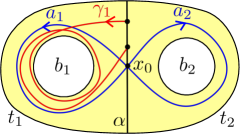
Figure 21. Illustration of the proof of 10.4 for pair of pants.

The geodesic $\gamma$ fills $P$, and is in particular not simple. As a consequence, it must intersect $\alpha$ (because $P\setminus\alpha$ is a union of two cylinders). All of its intersections are transversal, because $\gamma$ cannot coincide with $\alpha$ on an interval. The number of these intersections must be even because $\alpha$ separates $P$ into two connected components. We can therefore write $\gamma$ as the concatenation $\gamma_{1}\mathord{\mathchoice{\,\vbox{\hbox{\scalebox{0.5}{$\displaystyle\bullet$}}}\,}{\,\vbox{\hbox{\scalebox{0.5}{$\textstyle\bullet$}}}\,}{\,\vbox{\hbox{\scalebox{0.5}{$\scriptstyle\bullet$}}}\,}{\,\vbox{\hbox{\scalebox{0.5}{$\scriptscriptstyle\bullet$}}}\,}}\gamma_{2}\mathord{\mathchoice{\,\vbox{\hbox{\scalebox{0.5}{$\displaystyle\bullet$}}}\,}{\,\vbox{\hbox{\scalebox{0.5}{$\textstyle\bullet$}}}\,}{\,\vbox{\hbox{\scalebox{0.5}{$\scriptstyle\bullet$}}}\,}{\,\vbox{\hbox{\scalebox{0.5}{$\scriptscriptstyle\bullet$}}}\,}}\ldots\mathord{\mathchoice{\,\vbox{\hbox{\scalebox{0.5}{$\displaystyle\bullet$}}}\,}{\,\vbox{\hbox{\scalebox{0.5}{$\textstyle\bullet$}}}\,}{\,\vbox{\hbox{\scalebox{0.5}{$\scriptstyle\bullet$}}}\,}{\,\vbox{\hbox{\scalebox{0.5}{$\scriptscriptstyle\bullet$}}}\,}}\gamma_{2k}$, where for every $i$, $\gamma_{i}$ is a geodesic path intersecting $\alpha$ exactly at its endpoints, lying entirely on the connected component of $P\setminus\alpha$ containing $b_{\bar{\imath}}$ for $\bar{\imath}\in\{1,2\}$ of the same parity as $i$.

The path $\alpha$ cuts $b_{3}$ into two geodesic arcs, of respective lengths $t_{1}$ and $t_{2}$. For all $i$, the geodesic path $\gamma_{i}$ is a path from $\alpha$ to itself on the connected component $C_{\bar{\imath}}$ of $P$ containing $b_{\bar{\imath}}$, that cannot be homotoped to a sub-path of $\alpha$ (by minimality of the length of $\gamma$ in its homotopy class). As a consequence, its length is greater than the length $t_{\bar{\imath}}$ of the path minimising this property. We deduce that

$$A\log(g)\geq\ell_{X}(\gamma)=\sum_{i=1}^{2k}\ell(\gamma_{i})\geq k(t_{1}+t_{2})\geq k\,\kappa\log(g),$$

which implies that $k\leq A/\kappa$.

For all $i$, $\gamma_{i}$ is homotopic with endpoints gliding along $\alpha$ to $a_{\bar{\imath}}^{m_{i}}$ for an integer $m_{i}\in\mathbb{Z}$. The component $C_{\bar{\imath}}$ is isometric to part of a hyperbolic cylinder of core of length $\geq\kappa$. Projecting the geodesic path $\gamma_{i}$ on the core $b_{\bar{\imath}}$ following Fermi coordinates decreases its length, and in doing so we obtain a path on $b_{\bar{\imath}}$ rotating at least $|m_{i}|-1$ times around it. It follows that

$$A\log(g)\geq\ell(\gamma_{i})\geq(|m_{i}|-1)\kappa,$$

which implies that $|m_{i}|\leq M:=1+\lceil\frac{A}{\kappa}\log g\rceil$.

To conclude, we have proven that $\gamma$ is freely homotopic to $a_{1}^{m_{1}}\mathord{\mathchoice{\,\vbox{\hbox{\scalebox{0.5}{$\displaystyle\bullet$}}}\,}{\,\vbox{\hbox{\scalebox{0.5}{$\textstyle\bullet$}}}\,}{\,\vbox{\hbox{\scalebox{0.5}{$\scriptstyle\bullet$}}}\,}{\,\vbox{\hbox{\scalebox{0.5}{$\scriptscriptstyle\bullet$}}}\,}}a_{2}^{m_{2}}\mathord{\mathchoice{\,\vbox{\hbox{\scalebox{0.5}{$\displaystyle\bullet$}}}\,}{\,\vbox{\hbox{\scalebox{0.5}{$\textstyle\bullet$}}}\,}{\,\vbox{\hbox{\scalebox{0.5}{$\scriptstyle\bullet$}}}\,}{\,\vbox{\hbox{\scalebox{0.5}{$\scriptscriptstyle\bullet$}}}\,}}\ldots\mathord{\mathchoice{\,\vbox{\hbox{\scalebox{0.5}{$\displaystyle\bullet$}}}\,}{\,\vbox{\hbox{\scalebox{0.5}{$\textstyle\bullet$}}}\,}{\,\vbox{\hbox{\scalebox{0.5}{$\scriptstyle\bullet$}}}\,}{\,\vbox{\hbox{\scalebox{0.5}{$\scriptscriptstyle\bullet$}}}\,}}a_{1}^{m_{2k-1}}\mathord{\mathchoice{\,\vbox{\hbox{\scalebox{0.5}{$\displaystyle\bullet$}}}\,}{\,\vbox{\hbox{\scalebox{0.5}{$\textstyle\bullet$}}}\,}{\,\vbox{\hbox{\scalebox{0.5}{$\scriptstyle\bullet$}}}\,}{\,\vbox{\hbox{\scalebox{0.5}{$\scriptscriptstyle\bullet$}}}\,}}a_{2}^{m_{2k}}$ for $k:=\lceil A/\kappa\rceil$ and a family of integers $(m_{i})_{1\leq i\leq k}$ such that $|m_{i}|\leq M$ for all $i$. We put all of those local topologies in the set $\mathrm{Loc}_{g}^{\kappa,A}$, and note that the number of such configurations is bounded by

$$(2M+1)^{2k}=\mathcal{O}_{\kappa,A}\left((\log g)^{\lceil 2A/\kappa\rceil}\right).$$

The proof in the case of a once-holed torus is similar. ∎

10.2. Inclusion-exclusion

In order to be able to “make the assumption that $X\in\mathcal{A}_{g}^{\kappa}$”, we need to be able to compute expectations of functions in which the indicator function $\mathds{1}_{\mathcal{A}_{g}^{\kappa}}=\mathds{1}_{N_{\kappa}^{\mathrm{inj}}=0}\times\mathds{1}_{N_{\kappa}^{\mathrm{tang}}=0}$ appears. A good way to achieve this is to write this indicator function in terms of counting functions, using an inclusion-exclusion (such an argument also appears in Friedman’s proof of Alon’s conjecture [10]). The hope is that these counting functions can then be expressed in terms of geometric functions and integrated using Mirzakhani’s integration formula.

The indicator function $\mathds{1}_{N_{\kappa}^{\mathrm{inj}}=0}$ can be rewritten in the following way, as done by Mirzakhani [27] and Lipnowski–Wright [21].

Notation 10.5.

For $j\geq 1$, we define

$$N_{\kappa,j}^{\mathrm{inj}}(X)=\#\{\text{unordered families }\{\beta_{1},\ldots,\beta_{j}\}\text{ of distinct }\kappa\text{-short-loops on }X\}.$$

Lemma 10.6.

For any small enough $\kappa>0$, for any $j\geq 1$, all families of geodesics counted by $N_{\kappa,j}^{\mathrm{inj}}$ are made of simple and disjoint geodesics, and

(10.2) $$\mathds{1}_{N_{\kappa}^{\mathrm{inj}}=0}=1-\sum_{j=1}^{+\infty}(-1)^{j+1}N_{\kappa,j}^{\mathrm{inj}}=\sum_{j=0}^{+\infty}(-1)^{j}N_{\kappa,j}^{\mathrm{inj}}$$

with the convention that $N_{\kappa,0}^{\mathrm{inj}}=1$.

Proof.

We simply observe that, by the binomial theorem,

$$\forall n\geq 0,\quad\sum_{j=0}^{n}(-1)^{j}\binom{n}{j}=\begin{cases}1&\text{if }n=0\\ 0&\text{otherwise.}\end{cases}$$

The fact that the geodesics are simple and disjoint for small enough $\kappa$ is a classic application of the Collar Lemma [7, Theorem 4.1.6]. ∎

However, there is no reason to believe that all embedded surfaces contributing to $N_{\kappa}^{\mathrm{tang}}$ are disjoint. For this reason, it is a priori better to treat the indicator function of $N_{\kappa}^{\mathrm{tang}}=0$ differently, to avoid a tedious enumeration of cases. Luckily, the following easy inclusion-exclusion is enough for proving 10.1.

Notation 10.7.

We define

$$N_{\kappa,2}^{\mathrm{tang}}:=\#\{\text{unordered pairs }\{Y,Y^{\prime}\}\text{ of distinct }\kappa\text{-tangles on }X\}.$$

Lemma 10.8.

For any $\kappa>0$ and $g\geq 2$,

$$\mathds{1}_{N_{\kappa}^{\mathrm{tang}}=0}=1-N_{\kappa}^{\mathrm{tang}}+\mathcal{O}\left(N_{\kappa,2}^{\mathrm{tang}}\right).$$

Proof.

The bound is a direct consequence of the inequality $0\leq N_{\kappa}^{\mathrm{tang}}-\mathds{1}_{N_{\kappa}^{\mathrm{tang}}\geq 1}\leq N_{\kappa,2}^{\mathrm{tang}}$, which is trivially true when $X$ contains $0$ or $1$ tangles, and otherwise true because

$$\forall n\geq 2,\quad 0\leq n-1\leq\frac{n(n-1)}{2}=\binom{n}{2}.$$

∎

10.3. Expression of the terms arising in the inclusion-exclusion

The aim of this section is to express sums of the form

$$\mathbb{E}_{g}^{\mathrm{\scriptsize{WP}}}\Bigg{[}\sum_{\gamma}F(\ell_{X}(\gamma))\,\mathds{1}_{\mathcal{A}_{g}^{\kappa}}(X)\Bigg{]},$$

where the sum runs over all $\gamma\in\mathcal{P}_{g}$ or $\gamma\in T^{g}$ for a local type $T$, under a manageable form, using the formulas for $\mathds{1}_{\mathcal{A}_{g}^{\kappa}}$ from Section 10.2.

We proceed in three steps, presented in the following three paragraphs:

• first, we prove an upper bound in all expectations involving $N_{\kappa,2}^{\mathrm{tang}}$, which will allow us to neglect such terms in the proof of 10.1;

• then, we estimate $\mathbb{E}_{g}^{\mathrm{\scriptsize{WP}}}\left[\sum_{\gamma\in T^{g}}F(\ell_{X}(\gamma))\,\mathds{1}_{N_{\kappa}^{\mathrm{inj}}=0}(X)\right]$, up to reasonable errors, for the local type “simple” and any local type filling a pair of pants;

• finally, we estimate $\mathbb{E}_{g}^{\mathrm{\scriptsize{WP}}}\left[\sum_{\gamma\in T^{g}}F(\ell_{X}(\gamma))\,\mathds{1}_{N_{\kappa}^{\mathrm{inj}}=0}(X)N_{\kappa}^{\mathrm{tang}}(X)\right]$, up to reasonable errors, for the same local types as above.

This will be enough because

(10.3) $$\mathds{1}_{\mathcal{A}_{g}^{\kappa}}=\mathds{1}_{N_{\kappa}^{\mathrm{inj}}=0}-\mathds{1}_{N_{\kappa}^{\mathrm{inj}}=0}N_{\kappa}^{\mathrm{tang}}+\mathcal{O}\left(N_{\kappa,2}^{\mathrm{tang}}\right).$$

10.3.1. Expectation against $N_{\kappa,2}^{\mathrm{tang}}$

The following lemma will allow us to discard any expectation in which $N_{\kappa,2}^{\mathrm{tang}}$ appears when proving the $2/9-\epsilon$ spectral gap result. This is the reason why the writing in 10.8 is enough for our purposes. We expect a more careful inclusion-exclusion to be necessary to reach the optimal spectral gap $1/4-\epsilon$.

Lemma 10.9.

For any $0<\kappa<1$, any large enough $g$, any admissible function $F$, if $L:=6\log(g)$, then

$$\mathbb{E}_{g}^{\mathrm{\scriptsize{WP}}}\Bigg{[}\sum_{\begin{subarray}{c}\gamma\in\mathcal{P}_{g}\\ \ell_{X}(\gamma)\leq L\end{subarray}}F(\ell_{X}(\gamma))\,N_{\kappa,2}^{\mathrm{tang}}(X)\Bigg{]}=\mathcal{O}_{\kappa}\left(\frac{\|F(\ell)\exp(\ell)\|_{\infty}}{g^{2-19\kappa}}\right).$$

Proof.

First, we notice that, using the triangle inequality, we can consider the case $F(x)=e^{-x}$ only. Let $\gamma$ be a closed geodesic on $X$ of length $\leq L$, and $Y$, $Y^{\prime}$ be two distinct tangles on $X$. Let $S:=S_{\gamma}$ be the surface filled by $\gamma$. We define $S^{\prime}$ to be the surface obtained by adding any disk in the complement of the union $S\cup Y\cup Y^{\prime}$. The surface $S^{\prime}$ is not necessarily connected, and has at most three connected components. Because the boundary of $S^{\prime}$ can be obtained from the boundary of $S$ together with $\partial Y$ and $\partial Y^{\prime}$, we have

(10.4) $$\ell_{X}(\partial S^{\prime})\leq\ell_{X}(\partial S)+6\kappa\log(g)\leq 2\ell_{X}(\gamma)+6\log(g)\leq 18\log(g)=3L.$$

We observe that the surface $S^{\prime}$ contains the surface $Y$ of Euler characteristic $-1$. Furthermore, $S^{\prime}\neq Y$, because $S^{\prime}$ contains $Y^{\prime}$ and $Y\neq Y^{\prime}$. Since $S^{\prime}\setminus Y$ cannot be reduced to one cylinder (by definition of the notion of tangle), $r:=-\chi_{S^{\prime}}\geq 2$.

As in the proof of 6.3, we use the generalised tangle-free hypothesis developed in Section 6.3 to bound the number of possibilities for the Euler characteristic $-r$. Indeed, for an integer $N\geq 1$, let $\mathcal{B}_{g}^{(N)}\subset\mathcal{M}_{g}$ denote the set of $(N,\log(g))$-tangle-free surfaces. Then, we have the following bounds.

• By 6.7, $1-\mathbb{P}_{g}^{\mathrm{\scriptsize{WP}}}\left(\mathcal{B}_{g}^{(N)}\right)=\mathcal{O}_{N}\left(1/g^{N/2-1}\right)$.

• By the naive geodesic-counting result, 2.1, for any $X\in\mathcal{M}_{g}$,

  • $N_{\kappa,2}^{\mathrm{tang}}(X)=\mathcal{O}\left(g^{6(\kappa+1)}\right)$ because the pair of tangle is determined by at most $6$ geodesics of lengths $\leq\kappa\log(g)$;

  • $\sum_{\begin{subarray}{c}\gamma:\ell_{X}(\gamma)\leq L\end{subarray}}e^{-\ell_{X}(\gamma)}=\mathcal{O}\left(Lg\right)$.

As a consequence, taking $N:=34$, for any $\kappa<1$,

(10.5) $$\mathbb{E}_{g}^{\mathrm{\scriptsize{WP}}}\Bigg{[}\sum_{\begin{subarray}{c}\gamma\in\mathcal{P}_{g}\\ \ell_{X}(\gamma)\leq L\end{subarray}}e^{-\ell_{X}(\gamma)}\,N_{\kappa,2}^{\mathrm{tang}}(X)(1-\mathds{1}_{\mathcal{B}_{g}^{(N)}}(X))\Bigg{]}=\mathcal{O}_{N}\left(\frac{Lg^{7+6\kappa}}{g^{N/2-1}}\right)=\mathcal{O}\left(\frac{1}{g^{2}}\right).$$

We now apply 6.12 to obtain that, as soon as $\kappa<1/16$, there exists a universal constant $M$ such that, for any $\gamma,Y,Y^{\prime}$ with a non-zero contribution to the sum

(10.6) $$\mathbb{E}_{g}^{\mathrm{\scriptsize{WP}}}\Bigg{[}\sum_{\begin{subarray}{c}\gamma\in\mathcal{P}_{g}\\ \ell_{X}(\gamma)\leq L\end{subarray}}e^{-\ell_{X}(\gamma)}\,N_{\kappa,2}^{\mathrm{tang}}(X)\,\mathds{1}_{\mathcal{B}_{g}^{(N)}}(X)\Bigg{]},$$

the Euler characteristic of the connected component of $S^{\prime}$ containing $\gamma$ is smaller than $M$ in absolute value. Because the other connected components of $S^{\prime}$ are tangles, of Euler characteristic $-1$, this implies that $r\leq M+2$. We can therefore reduce the sum (10.6) to only contributions such that $2\leq r\leq M+2$. Then, by positivity, we can remove the indicator function $\mathds{1}_{\mathcal{B}_{g}^{(N)}}\leq 1$, and hence obtain

(10.7) $$\mathbb{E}_{g}^{\mathrm{\scriptsize{WP}}}\Bigg{[}\sum_{\begin{subarray}{c}\gamma\in\mathcal{P}_{g}\\ \ell_{X}(\gamma)\leq L\end{subarray}}e^{-\ell_{X}(\gamma)}\,N_{\kappa,2}^{\mathrm{tang}}(X)\,\mathds{1}_{\mathcal{B}_{g}^{(N)}}\Bigg{]}\leq\sum_{r=2}^{M+2}\mathbb{E}_{g}^{\mathrm{\scriptsize{WP}}}\Bigg{[}\sum_{\begin{subarray}{c}(\gamma,Y,Y^{\prime})\\ \ell_{X}(\gamma)\leq L\\ \chi_{S^{\prime}}=-r\end{subarray}}e^{-\ell_{X}(\gamma)}\Bigg{]}$$

where the sum runs over all families $(\gamma,Y,Y^{\prime})$ such that $\gamma$ is a primitive closed geodesic on $X$ of length $\leq 6\log(g)$, $Y$ and $Y^{\prime}$ are disjoint tangles on $X$, and $\chi_{S^{\prime}}=-r$.

Let us fix a filling type $S^{\prime}$ of Euler characteristic $2\leq r\leq M+2$, with at most three connected components, and a connected subsurface $S\subset S^{\prime}$ (we allow that $S$ is a connected component of $S^{\prime}$, or shares some of its boundary components). By (10.4), the quantity we need to bound is smaller than

(10.8) $$\mathbb{E}_{g}^{\mathrm{\scriptsize{WP}}}\Bigg{[}\sum_{\begin{subarray}{c}(Z,Z^{\prime})\text{ on }S_{g}\\ \text{ homeo to }(S,S^{\prime})\\ \ell_{X}(\partial Z),\ell_{X}(\partial Z^{\prime})\leq 3L\end{subarray}}N_{\kappa,2}^{\mathrm{tang}}(Z^{\prime})\sum_{\begin{subarray}{c}\gamma\text{ filling }Z\\ \ell_{X}(\gamma)\leq L\end{subarray}}e^{-\ell_{X}(\gamma)}\mathds{1}_{\ell_{X}(\partial Z^{\prime})\leq\ell_{X}(\partial Z)+6\kappa\log(g)}\Bigg{]}.$$

We once again use 2.1 to bound the number of pairs of tangles, and obtain that for any $Z^{\prime}$ as above, $N_{\kappa,2}^{\mathrm{tang}}(Z^{\prime})=\mathcal{O}\left((re^{\kappa\log(g)})^{6}\right)=\mathcal{O}\left(g^{6\kappa}\right)$. We use 2.3 with $\eta=\kappa$ to bound the number of possibilities for the loop $\gamma$ filling $Z$, and obtain that

$$\sum_{\begin{subarray}{c}\gamma\text{ filling }Z\\ \ell_{X}(\gamma)\leq L\end{subarray}}e^{-\ell_{X}(\gamma)}=\mathcal{O}_{\kappa}\left(Le^{-\frac{1-\kappa}{2}\ell_{X}(\partial Z)}\right)=\mathcal{O}_{\kappa}\left(g^{12\kappa}\exp\left(-\frac{\ell_{X}(\partial Z^{\prime})}{2}\right)\right)$$

because, by the hypotheses on the lengths of $\partial Z$ and $\partial Z^{\prime}$ in (10.8),

$$\frac{1-\kappa}{2}\ell_{X}(\partial Z)\geq\frac{1-\kappa}{2}\ell_{X}(\partial Z^{\prime})-3\kappa(1-\kappa)\log(g)>\frac{\ell_{X}(\partial Z^{\prime})}{2}-12\kappa\log(g).$$

Therefore,

$$\eqref{eq:proof_Ntang_2_enumeration}=\mathcal{O}_{\kappa}\Bigg{(}g^{18\kappa}\mathbb{E}_{g}^{\mathrm{\scriptsize{WP}}}\Bigg{[}\sum_{\begin{subarray}{c}(Z,Z^{\prime})\text{ on }S_{g}\\ \text{ homeo to }(S^{\prime}S^{\prime})\\ \ell_{X}(\partial Z),\ell_{X}(\partial Z^{\prime})\leq 3L\end{subarray}}\exp\left(-\frac{\ell_{X}(\partial Z^{\prime})}{2}\right)\Bigg{]}\Bigg{)}.$$

We use Mirzakhani’s integration formula to compute this expectation, and obtain that we need to bound

(10.9) $$g^{18\kappa}\int_{\begin{subarray}{c}\lVert\mathbf{x}\rVert_{1},\lVert\mathbf{y}\rVert_{1}\leq 3L\end{subarray}}\phi_{g}^{S^{\prime}}(\mathbf{x})\frac{V_{S}(\mathbf{y})V_{S^{\prime}\setminus S}(\mathbf{x},\mathbf{y})}{V_{S^{\prime}}(\mathbf{x})}\exp\left(-\frac{\lVert\mathbf{x}\rVert_{1}}{2}\right)\,\mathrm{d}\mathbf{x}\,\mathrm{d}\mathbf{y}$$

where

• $\mathbf{x}$ denotes the length-vector of $\partial Z^{\prime}$ and $\mathbf{y}$ that of $\partial Z$;

• $\lVert\cdot\rVert_{1}$ is the $\ell^{1}$-norm on $\mathbb{R}^{p}$ for $p\geq 1$;

• $\phi_{g}^{S^{\prime}}$ is sum over all realisations of $S^{\prime}$ in $S_{g}$ as introduced in (5.4) for connected filling types, and generalised in Section 5.5 to more general filling types;

• $V_{S}(\mathbf{y})$, $V_{S^{\prime}}(\mathbf{x})$ and $V_{S^{\prime}\setminus S}(\mathbf{x},\mathbf{y})$ respectively stand for the product of the Weil–Petersson volumes of the components of $S$, $S^{\prime}$ and $S^{\prime}\setminus S$.

We bound the Weil–Petersson volumes $V_{S}(\mathbf{y})$ and $V_{S^{\prime}\setminus S}(\mathbf{x},\mathbf{y})$ by the polynomial bound (2.6), and note that their values for $\mathbf{x}=\mathbf{0}$ and $\mathbf{y}=\mathbf{0}$ are $\mathcal{O}\left(1\right)$ because $r\leq M+2$. We naturally extend the bound on $\phi_{g}^{S^{\prime}}$ from 5.21 with $K=r=|\chi_{S^{\prime}}|$ to the case of disconnected filling types. Altogether, this allows us to deduce that (10.9) is $\mathcal{O}\left(g^{18\kappa-r}(3L)^{c(r)}\right)$ for a constant $c(r)$ depending only on $r$.

Summing these inequalities for $2\leq r\leq M+2$, we obtain that (10.6) is $\mathcal{O}_{\kappa}\left(g^{19\kappa-2}\right)$, which together with (10.5) leads to our claim. ∎

10.3.2. Expectation against $\mathds{1}_{N_{\kappa}^{\mathrm{inj}}=0}$

For a local topological type $T$, $g\geq 2$, an admissible function $F$ and a set $\mathcal{A}_{g}\subset\mathcal{M}_{g}$, we denote

$$\langle F\,|\,X\in\mathcal{A}_{g}\rangle_{g}^{{T}}:=\mathbb{E}_{g}^{\mathrm{\scriptsize{WP}}}\Bigg{[}\sum_{\gamma\in T^{g}}F(\ell_{X}(\gamma))\,\mathds{1}_{\mathcal{A}_{g}}(X)\Bigg{]}$$

and we naturally define $\langle F\,|\,X\in\mathcal{A}_{g}\rangle_{g}^{{\mathrm{all}}}$ the same way. The aim of this section is to provide expressions for these averages for $\mathcal{A}_{g}=\{X\in\mathcal{M}_{g}\,:\,N_{\kappa}^{\mathrm{inj}}(X)=0\}$, in particular when $T$ is the local type “simple” or a local type filling a pair of pants. This requires some of the notations introduced in Section 5.5, generalising the notion of local topological type and average over a local type to situations where the surface is not connected, or filled by several loops. We prove the following.

Lemma 10.10.

There exists a constant $c>0$ such that, for any small enough $\kappa>0$, any large enough $g$, $L:=6\log(g)$, any admissible function $F$ of support in $[0,L]$,

1. for the local topological type “simple”,

   (10.10) $$\begin{split}\langle F\,|\,N_{\kappa}^{\mathrm{inj}}=0\rangle_{g}^{{\mathrm{s}}}=&\sum_{j=0}^{+\infty}\frac{(-1)^{j}}{j!}\Bigg{(}\langle F,\mathds{1}_{[0,\kappa]}^{j}\rangle_{g}^{{\mathrm{s}^{j+1}}}-\sum_{T\in\mathcal{T}_{1,1}^{2\mathrm{s}}}\langle(F,\mathds{1}_{[0,\kappa]}),\mathds{1}_{[0,\kappa]}^{j}\rangle_{g}^{{T\times\mathrm{s}^{j}}}\Bigg{)}\\ &+\mathcal{O}_{\kappa}\left(\|F\|_{\infty}+\frac{\|F(\ell)\,e^{\ell}\|_{\infty}}{g^{2-c\kappa}}\right)\end{split}$$

   where for any $j\geq 0$,

   • $\mathrm{s}^{j}=(\mathrm{s},\ldots,\mathrm{s})$ is the local topology with $j$ copies of the type “simple”;

   • $\mathcal{T}_{1,1}^{2\mathrm{s}}$ is the set of local topological types of pairs of simple loops filling $S_{1,1}$.

2. for any local type $T$ filling a pair of pants,

   (10.11) $$\langle F\,|\,N_{\kappa}^{\mathrm{inj}}=0\rangle_{g}^{{T}}=\sum_{j=0}^{+\infty}\frac{(-1)^{j}}{j!}\langle F,\mathds{1}_{[0,\kappa]}^{j}\rangle_{g}^{{T\times\mathrm{s}^{j}}}+\mathcal{O}_{\kappa}\left(\|F\|_{\infty}+\frac{\|F(\ell)\,e^{\ell}\|_{\infty}}{g^{2-c\kappa}}\right).$$

Proof.

First, we observe that by the triangle inequality,

$$\left|\langle F\mathds{1}_{[0,\kappa]}\,|\,N_{\kappa}^{\mathrm{inj}}=0\rangle_{g}^{{\mathrm{all}}}\right|\leq\|F\|_{\infty}\,\mathbb{E}_{g}^{\mathrm{\scriptsize{WP}}}\left[\#\{\gamma\in\mathcal{P}_{g}\,:\,\ell_{X}(\gamma)\leq\kappa\}\right]=\mathcal{O}\left(\kappa^{2}\|F\|_{\infty}\right)$$

by [27, Section 4.2]. We can therefore restrict both sums we wish to study to geodesics $\gamma$ of length $>\kappa$. We then apply 10.6, which tells us that for small enough $\kappa$, all geodesics of length $\leq\kappa$ are disjoint, and that we can write

$$\langle F\mathds{1}_{(\kappa,L]}\,|\,N_{\kappa}^{\mathrm{inj}}=0\rangle_{g}^{{\mathrm{s}}}=\sum_{j=0}^{+\infty}(-1)^{j}\,\mathbb{E}_{g}^{\mathrm{\scriptsize{WP}}}\Bigg{[}\sum_{\begin{subarray}{c}\gamma\text{ simple}\\ \kappa<\ell_{X}(\gamma)\leq L\end{subarray}}F(\ell_{X}(\gamma))\,N_{\kappa,j}^{\mathrm{inj}}(X)\Bigg{]}.$$

For any $j\geq 0$, we pick a numbering of the $j$-tuples counted in $N_{\kappa,j}^{\mathrm{inj}}$, which allows us to rewrite the sum above as

(10.12) $$\sum_{j=0}^{+\infty}\frac{(-1)^{j}}{j!}\,\mathbb{E}_{g}^{\mathrm{\scriptsize{WP}}}\Bigg{[}\sum_{\begin{subarray}{c}\gamma\text{ simple}\\ \kappa<\ell_{X}(\gamma)\leq L\end{subarray}}\sum_{\begin{subarray}{c}(\beta_{1},\ldots,\beta_{j})\end{subarray}}F(\ell_{X}(\gamma))\prod_{i=1}^{j}\mathds{1}_{[0,\kappa]}(\ell_{X}(\beta_{i}))\Bigg{]}.$$

We notice that the hypothesis $\ell_{X}(\gamma)>\kappa$ implies that $\gamma$ is distinct from $\beta_{i}^{\pm 1}$ for all $i$. As in the proof of 10.9, we regroup the terms of this sum according to the topology of the surface $S^{\prime}$ filled by the multi-loop $(\gamma,\beta_{1},\ldots,\beta_{j})$. This allows us to prove, using the same strategy, that there exists a constant $c>0$ such that the restriction of equation 10.12 to multi-loops such that $|\chi_{S^{\prime}}|\geq 2$ is $\mathcal{O}_{\kappa}\left(\|F(\ell)\,e^{\ell}\|_{\infty}/g^{2-c\kappa}\right)$. Hence, we only need to enumerate local topologies for which $|\chi_{S^{\prime}}|\leq 1$.

The only local topology for which $\chi_{S^{\prime}}=0$ is the product $\mathrm{s}^{j+1}$ of $j+1$ copies of the local type “simple”. By definition of the average $\langle\cdot\rangle_{g}^{{\mathrm{s}^{j+1}}}$, these contributions can be rewritten as

$$\sum_{j=0}^{+\infty}\frac{(-1)^{j}}{j!}\langle F,\mathds{1}_{[0,\kappa]},\ldots,\mathds{1}_{[0,\kappa]}\rangle_{g}^{{\mathrm{s}^{j+1}}}.$$

This is the first term on the right hand side of equation 10.10.

Now, we carefully enumerate the local topologies for which $\chi_{S^{\prime}}=-1$. We recall that, by hypothesis on $\kappa$, for any multi-loop $(\gamma,\beta_{1},\ldots,\beta_{j})$ contributing to the sum, all the $\beta_{j}$ are simple and disjoint. Furthermore, $\gamma$ is simple, and distinct from any $\beta_{i}^{\pm 1}$ (but not necessarily disjoint). The only way to obtain a local type of Euler characteristic $-1$ then is to take a type $T\times\mathrm{s}^{j-k}$, where $T=[S_{1,1},(\gamma,\beta_{i_{1}},\ldots,\beta_{i_{k}})]_{\mathrm{loc}}$ or $[S_{0,3},(\gamma,\beta_{i_{1}},\ldots,\beta_{i_{k}})]_{\mathrm{loc}}$ for a $k\leq j$ and a multi-loop $(\gamma,\beta_{i_{1}},\ldots,\beta_{i_{k}})$ filling $S_{1,1}$ or $S_{0,3}$.

• Any simple loop on the pair of pants $S_{0,3}$ is homotopic to one of its boundary components. It is therefore impossible to fill a pair of pants with a multi-loop containing only simple loops, so the case $S_{0,3}$ cannot happen.

• If $T=[S_{1,1},(\gamma,\beta_{i_{1}},\ldots,\beta_{i_{k}})]_{\mathrm{loc}}$, in order for the multi-loop to fill the once-holed torus, we need $k\geq 1$, because $\gamma$ is simple. But a once-holed torus cannot contain two disjoint essential curves, so $k=1$. After the change of variables $j\rightarrow j-1$, counting the number of possibilities for the choice of the index $i_{1}$, this yields the second term on the right hand side of equation 10.10.

This allows us to conclude. The proof in the case of a local topology $T$ filling a pair of pants $P$ is the same, with less cases because the only thing we can add to $P$ to form a $S^{\prime}$ of Euler characteristic $-1$ is cylinders. ∎

10.3.3. Expectation against $\mathds{1}_{N_{\kappa}^{\mathrm{inj}}}\times N_{\kappa}^{\mathrm{tang}}$

Let us conclude this section with the last cases that need to be described to compute averages of the form $\langle F\,|\,X\in\mathcal{A}_{g}^{\kappa}\rangle_{g}^{{T}}$, in light of equation 10.3.

Lemma 10.11.

There exists a constant $c>0$ such that, for any small enough $\kappa>0$, any large enough $g$, $L:=6\log(g)$, any admissible function $F$ of support in $[0,L]$,

(10.13) $$\begin{split}&\quad\mathbb{E}_{g}^{\mathrm{\scriptsize{WP}}}\Bigg{[}\sum_{\begin{subarray}{c}\gamma\text{ simple}\\ \ell_{X}(\gamma)\leq L\end{subarray}}F(\ell_{X}(\gamma))\,\mathds{1}_{N_{\kappa}^{\mathrm{inj}}=0}(X)\,N_{\kappa}^{\mathrm{tang}}(X)\Bigg{]}\\ &=\sum_{j=0}^{+\infty}\frac{(-1)^{j}}{j!}\Bigg{(}\langle F,\mathds{1}_{[0,\kappa]}^{j},\mathds{1}_{[0,\kappa\log(g)]}^{3}\rangle_{g}^{{\mathrm{s}^{j+1}\times T_{0,3}^{b}}}+\langle F,\mathds{1}_{[0,\kappa]}^{j},\mathds{1}_{[0,\kappa\log(g)]}\rangle_{g}^{{\mathrm{s}^{j+1}\times T_{1,1}^{b}}}\Bigg{)}\\ &+\sum_{j=0}^{+\infty}\frac{(-1)^{j}}{j!}\Bigg{(}\langle(F,\mathds{1}_{[0,\kappa\log(g)]}),\mathds{1}_{[0,\kappa]}^{j}\rangle_{g}^{{T_{1,1}^{1,b}\times\mathrm{s}^{j}}}-\sum_{T\in\mathcal{T}_{1,1}^{2\mathrm{s},b}}\langle(F,\mathds{1}_{[0,\kappa]},\mathds{1}_{[0,\kappa\log(g)]}),\mathds{1}_{[0,\kappa]}^{j}\rangle_{g}^{{T\times\mathrm{s}^{j}}}\Bigg{)}\\ &+\mathcal{O}_{\kappa}\left(\|F\|_{\infty}+\frac{\|F(\ell)e^{\ell}\|_{\infty}}{g^{2-c\kappa}}\right)\end{split}$$

and for any local topology $T$ filling a pair of pants,

(10.14) $$\begin{split}&\mathbb{E}_{g}^{\mathrm{\scriptsize{WP}}}\Bigg{[}\sum_{\begin{subarray}{c}\gamma\in T^{g}\\ \ell_{X}(\gamma)\leq L\end{subarray}}F(\ell_{X}(\gamma))\,\mathds{1}_{N_{\kappa}^{\mathrm{inj}}=0}(X)\,N_{\kappa}^{\mathrm{tang}}(X)\Bigg{]}\\ &=\sum_{j=0}^{+\infty}\frac{(-1)^{j}}{j!}\langle(F,\mathds{1}_{[0,\kappa\log(g)]}^{3}),\mathds{1}_{[0,\kappa]}^{j}\rangle_{g}^{{T^{b}\times\mathrm{s}^{j}}}+\mathcal{O}_{\kappa}\left(\|F\|_{\infty}+\frac{\|F(\ell)e^{\ell}\|_{\infty}}{g^{2-c\kappa}}\right)\end{split}$$

where

• $T_{0,3}^{b}$ and $T_{1,1}^{b}$ are the local types of respective filling types $S$ for $S=S_{0,3}$ and $S_{1,1}$, with $\gamma=\partial S$ (and, in the average for $S=S_{0,3}$, excluding the possibility of gluing two distinct boundary components of $S_{0,3}$ together);

• $T_{1,1}^{1,b}$ is the local type $[S_{1,1},(\beta,\partial S_{1,1})]_{\mathrm{loc}}$ where $\beta$ is the essential simple closed loop on the once-holed torus $S_{1,1}$;

• $\mathcal{T}_{1,1}^{2\mathrm{s},b}$ is the set of local types $[S_{1,1},(\gamma,\beta,\partial S_{1,1})]_{\mathrm{loc}}$ where $(\gamma,\beta)$ are two simple loops on $S_{1,1}$;

• if $T=[S_{0,3},\gamma]_{\mathrm{loc}}$, then $T^{b}$ is the local topology $[S_{0,3},(\gamma,\partial S_{0,3})]_{\mathrm{loc}}$.

Proof.

The proof runs along the same lines as the proof of 10.10, with the difference that we now enumerate possibilities for the loop $\gamma$, the multi-curve $(\beta_{1},\ldots,\beta_{j})$ and the tangle $S_{0,3}$ or $S_{1,1}$. Note that possibilities are quite limited, because the Euler characteristic of the tangle is $-1$ and we can exclude all situations for which the total Euler characteristic is $<-1$. For instance, in the case of (10.14), the only term corresponds to the case where the tangle is $S_{\gamma}$. ∎

10.3.4. Writing of these expectations as Friedman–Ramanujan functions

We are now able to prove the following proposition. This will allow us to apply the properties of Friedman–Ramanujan functions, and in particular the cancellation argument presented in Section 3.4, in the context of the inclusion-exclusion.

Proposition 10.12.

There exists a constant $c>0$ satisfying the following. For any small enough $\kappa>0$, any large enough $g$, any local topology that $T$ is “simple” or fills a pair of pants, there exists a density function $A_{T,g}^{\kappa}:\mathbb{R}_{>0}\rightarrow\mathbb{R}$ such that, for any admissible function $F$ of support included in $[0,L]$ with $L:=6\log(g)$,

$$\langle F\,|\,X\in\mathcal{A}_{g}^{\kappa}\rangle_{g}^{{T}}=\int_{0}^{+\infty}F(\ell)\,A_{T,g}^{\kappa}(\ell)\,\mathrm{d}\ell+\mathcal{O}_{\kappa}\left(\frac{\|F(\ell)\,e^{\ell}\|_{\infty}}{g^{2-c\kappa}}+g^{c\kappa}\|F(\ell)e^{\frac{\ell}{2}}\|_{\infty}\right).$$

Furthermore, the function $\ell\mapsto\ell A_{T,g}^{\kappa}(\ell)$ is Friedman–Ramanujan in the weak sense, of degree and exponent $\leq c$, and norm and constant $\mathcal{O}_{\kappa}\left(g^{c\kappa}\right)$.

We will use the following lemma to prove 10.12.

Lemma 10.13.

For any integer $j\geq 0$, any large enough $g$,

$$\frac{\prod_{i}x_{i}\,V_{g-2-j,2j+3}(\mathbf{x})}{V_{g}} =\frac{V_{g-2-j,2j+3}}{V_{g}}\prod_{i}2\sinh\left(\frac{x_{i}}{2}\right)+\mathcal{O}\left(\frac{\lVert\mathbf{x}\rVert+1}{g^{2}}\prod_{i}x_{i}e^{\frac{x_{i}}{2}}\right)$$

$$\frac{\prod_{i}x_{i}\,V_{g-1-j,2j+1}(\mathbf{x})}{V_{g}} =\frac{V_{g-1-j,2j+1}}{V_{g}}\prod_{i}2\sinh\left(\frac{x_{i}}{2}\right)+\mathcal{O}\left(\frac{\lVert\mathbf{x}\rVert+1}{g^{2}}\prod_{i}x_{i}e^{\frac{x_{i}}{2}}\right)$$

and the ratios $V_{g-2-j,2j+3}/V_{g}$ and $V_{g-1-j,2j+1}/V_{g}$ are $\mathcal{O}\left(1/g\right)$. Furthermore,

$$\frac{\prod_{i}x_{i}\,V_{g-j,2j}(\mathbf{x})}{V_{g}}=\sum_{\mathbf{m}}c^{(g,j)}_{\mathbf{m}}\prod_{i}f_{m_{i}}(x_{i})+\mathcal{O}\left(\frac{(j+1)^{4}(\lVert\mathbf{x}\rVert+1)^{3}}{g^{2}}\prod_{i}x_{i}e^{\frac{x_{i}}{2}}\right)$$

where the sum runs over all families $(m_{i})_{i}$ of integers in $\{1,\ldots,4\}$, the coefficients $c^{(g,j)}_{\mathbf{m}}$ are bounded uniformly in $g$ and $j$, and

(10.15) $$f_{1}(x)=2\sinh\left(\frac{x}{2}\right)\quad f_{2}(x)=2x^{2}\sinh\left(\frac{x}{2}\right)\quad f_{3}(x)=x\cosh\left(\frac{x}{2}\right)\quad f_{4}(x)=x.$$

Proof.

The proof is immediate for $V_{g-2-j,2j+3}(\mathbf{x})$ and $V_{g-1-j,2j+1}(\mathbf{x})$, as it is a simple consequence of the first-order expansion (2.8) together with Weil–Petersson volume comparisons from [27]. Indeed, by [27, Lemma 3.2], there exists a constant $c$ such that, for any $g,n,j$, $V_{g-j,n+2j}\leq cV_{g,n}$. Therefore, $V_{g-2-j,2j+3}/V_{g}=\mathcal{O}\left(V_{g-2,3}/V_{g}\right)=\mathcal{O}\left(1/g\right)$, and same goes for $V_{g-1-j,2j+1}$.

However, for $V_{g-j,2j}(\mathbf{x})$, we need to use the explicit second-order expansion from [2, Theorem 3.1], stating that for $g,n\geq 1$,

(10.16) $$\begin{split}&\prod_{i}x_{i}V_{g,n}(\mathbf{x})\\ &=8\;V_{g-1,n+1}\sum_{i=1}^{n}\left[f_{3}(x_{i})+f_{4}(x_{i})-\frac{f_{2}(x_{i})}{16}-2f_{1}(x_{i})\right]\prod_{k\neq i}f_{1}(x_{k})\\ &-4V_{g,n-1}\sum_{1\leq i<j\leq n}\left[f_{3}(x_{i})f_{3}(x_{j})+f_{4}(x_{i})f_{4}(x_{j})-2\,f_{1}(x_{i})f_{1}(x_{j})\right]\prod_{k\notin\{i,j\}}f_{1}(x_{k})\\ &+V_{g,n}\prod_{1\leq k\leq n}f_{1}(x_{k})+\mathcal{O}_{n}\left(V_{g,n}\frac{(\lVert\mathbf{x}\rVert+1)^{3}\prod_{i}x_{i}}{(g+1)^{2}}\;\exp\left(\frac{x_{1}+\ldots+x_{n}}{2}\right)\right)\end{split}$$

with the notations of (10.15). As above, we use [27, Lemma 3.2] to compare all coefficients appearing in the expansion of $\prod_{i}x_{i}V_{g-j,2j}(\mathbf{x})/V_{g}$ to the ones for which $j=0$ or $1$, and hence obtain a uniform bound on the various volume ratios.

We further check the dependency of the implied constant that appears when applying (10.16) in terms of $j$, following the proof of [2, Theorem 3.1], and using the method above to bring any volume appearing down to the case $j=0$ or $1$. More precisely, with the numbering of [2]: in each step of this second-order expansion, we gain exactly two powers of $j+1$. Indeed, during the first order, we gain one power when summing the different terms in equation (22), and another using Lemma 2.9. The same two steps in the second-order expansion yield two other terms $j+1$, which altogether lead to the term $(j+1)^{4}$. ∎

Let us now prove 10.12.

Proof.

Let $T=[P,\gamma]_{\mathrm{loc}}$ for a loop $\gamma$ filling the pair of pants $P$. For $j\geq 0$, by 5.5, the average $(-1)^{j}\langle F,\mathds{1}_{[0,\kappa]}^{j}\rangle_{g}^{{T\times\mathrm{s}^{j}}}/j!$ present in (10.11) can be written

$$\frac{(-1)^{j}}{j!}\frac{1}{m(T)}\int_{\mathbb{R}_{>0}^{3}}\int_{[0,\kappa]^{j}}F(\mathfrak{L}_{\gamma}(\ell_{1},\ell_{2},\ell_{3}))\,\phi_{g}^{S_{0,3}\times S_{0,2}^{j}}(\ell_{1},\ell_{2},\ell_{3},\mathbf{x})\,\mathrm{d}\ell_{1}\,\mathrm{d}\ell_{2}\,\mathrm{d}\ell_{3}\,\mathrm{d}\mathbf{x}.$$

The filling type $S_{0,3}\times S_{0,2}^{j}$ has Euler characteristic $-1$, so when we replace the realisation function above by its main term, we obtain an approximation of $\langle F,\mathds{1}_{[0,\kappa]}\rangle_{g}^{{T\times\mathrm{s}^{j}}}$ at precision $1/g^{2}$. First, we compute the term of the connected realisation, which is the case when we glue a surface of signature $(g-2-j,2j+3)$ to the pair of pants $S_{0,3}$ and the $j$ copies of the cylinder $S_{0,2}$. This yields a density function

$$\frac{(-1)^{j}}{j!}\frac{1}{m(T)}\int_{\star}\int_{[0,\kappa]^{j}}\frac{V_{g-2-j,2j+3}(\ell_{1},\ell_{2},\ell_{3},x_{1},x_{1},\ldots,x_{j},x_{j})}{V_{g}}\ell_{1}\ell_{2}\ell_{3}\frac{\,\mathrm{d}\ell_{1}\,\mathrm{d}\ell_{2}\,\mathrm{d}\ell_{3}}{\,\mathrm{d}\ell}\prod_{i=1}^{j}x_{i}\,\mathrm{d}x_{i}$$

where the integral $\int_{\star}$ runs on the level-set $\{\mathfrak{L}_{\gamma}(\ell_{1},\ell_{2},\ell_{3})=\ell\}$. By 10.13, we only need to compute

$$\frac{(-1)^{j}}{j!}\frac{1}{m(T)}\frac{V_{g-2-j,2j+3}}{V_{g}}\int_{\star}\int_{[0,\kappa]^{j}}\prod_{i=1}^{3}2\sinh\left(\frac{\ell_{i}}{2}\right)\prod_{i=1}^{j}\frac{4}{x_{i}}\sinh^{2}\left(\frac{x_{i}}{2}\right)\frac{\,\mathrm{d}\ell_{1}\,\mathrm{d}\ell_{2}\,\mathrm{d}\ell_{3}}{\,\mathrm{d}\ell}\,\mathrm{d}\mathbf{x}$$

$$=\frac{(-1)^{j}I(\kappa)^{j}}{j!}\frac{1}{m(T)}\frac{V_{g-2-j,2j+3}}{V_{g}}\int_{\star}\prod_{i=1}^{3}f_{1}(\ell_{i})\frac{\,\mathrm{d}\ell_{1}\,\mathrm{d}\ell_{2}\,\mathrm{d}\ell_{3}}{\,\mathrm{d}\ell}$$

where $I(\kappa):=\int_{0}^{\kappa}4\sinh^{2}\left(\frac{x}{2}\right)\,\mathrm{d}x/x=\mathcal{O}\left(\kappa\right)$ for $\kappa\leq 1$. We sum the terms for the different values of $j$ to obtain the corresponding density (the sum converges because $V_{g-2-j,2j+3}/V_{g}=\mathcal{O}\left(1\right)$ by 10.13). We can similarly write the terms arising from the other realisations of minimal rank, which are obtained by adding some Dirac distributions. This yields additional terms, multiple of

$$\iint_{\{\mathfrak{L}_{\gamma}(\ell_{1},\ell_{2},\ell_{3})=\ell\}}f_{1}(\ell_{i})\,\ell_{j}\delta(\ell_{j}-\ell_{k})\frac{\,\mathrm{d}\ell_{1}\,\mathrm{d}\ell_{2}\,\mathrm{d}\ell_{3}}{\,\mathrm{d}\ell}\quad\text{for }\{i,j,k\}=\{1,2,3\}$$

but also, when we glue one or two cylinders from the types $\mathrm{s}^{j}$ to the pair of pants $P$,

$$\int_{\{\mathfrak{L}_{\gamma}(\ell_{1},\ell_{2},\ell_{3})=\ell\}}\prod_{i=1}^{3}f_{1}(\ell_{i})\prod_{i\in I}\mathds{1}_{[0,\kappa]}(\ell_{i})\frac{\,\mathrm{d}\ell_{1}\,\mathrm{d}\ell_{2}\,\mathrm{d}\ell_{3}}{\,\mathrm{d}\ell}\quad\text{for }I\subset\{1,2,3\},$$

or even a mixture of both, for instance if we glue two components of $P$ to the same cylinder of $\mathrm{s}^{j}$. We notice that $f_{1}$ and $f_{1}\mathds{1}_{[0,\kappa]}$ both satisfy

(10.17) $$\frac{f(\ell)}{\sinh\left(\frac{\ell}{2}\right)}=p(\ell)+\mathcal{O}_{\kappa}\left(g^{c\kappa}(\ell+1)^{k}e^{-\ell/2}\right)$$

for the polynomial $p=1$ or $0$ respectively, and the exponents $k=c=0$, because $\mathds{1}_{[0,\kappa]}=\mathcal{O}_{\kappa}\left(e^{-\ell/2}\right)$. Then, the results of Sections 7 and 8 applied to the local type $T$ allow us to conclude that these densities are indeed Friedman–Ramanujan in the weak sense. The bound on the degree and exponent follow from the fact that we systematically integrate only functions that are products of $f_{1}$ and $f_{1}\mathds{1}_{[0,\kappa]}$, i.e. there are $\leq 2^{3}$ possible products, and the uniformity in 8.1 with respect to the local type. The bounds throughout the computation above further allow us to bound the constant and remainder of the density by $\mathcal{O}_{\kappa}\left(1\right)$.

The computation is the same for the average (10.14) containing the counting function $N_{\kappa}^{\mathrm{tang}}$, with the difference that now, we sometimes multiply by the indicator function $\mathds{1}_{[0,\kappa\log(g)]}(\ell)=\mathcal{O}\left(g^{\kappa/2}e^{-\ell/2}\right)$ coming from the tangles, and hence there is $\leq 3^{3}$ possible products. The degree and exponent is therefore still $\mathcal{O}\left(1\right)$, but the bound on the norm and remainder is now $\mathcal{O}_{\kappa}\left(g^{3\kappa/2}\right)$, which is is enough to conclude in the case of a type $T$ filling a pair of pants.

Let us now consider the local topology “simple”. Similarly, we examine each term in (10.10) and (10.13) one after the other. For all the terms except the terms containing the summations over $\mathcal{T}_{1,1}^{2\mathrm{s}}$ and $\mathcal{T}_{1,1}^{2\mathrm{s},b}$, this allows us to express the product of the density and the function $\ell\mapsto\ell$ as a linear combination of functions $\ell\mapsto f^{(\kappa)}_{m_{1}}(\ell)f^{(\kappa)}_{m_{2}}(\ell)$ with bounded coefficients, where the family of functions $(f_{i}^{(\kappa)})_{1\leq i\leq 15}$ consists of all products of a function of equation 10.15 or $f_{5}(x):=x^{3}$ (coming from the expression of the volume $xV_{1,1}(x)$) with $1$, $\mathds{1}_{[0,\kappa]}$ and $\mathds{1}_{[0,\kappa\log(g)]}$. We check all of these functions satisfy the property (10.17), which is enough to conclude for these terms.

Now, the last cases we need to consider are the cases where we sum over local topological types $T$ in $\mathcal{T}_{1,1}^{2\mathrm{s}}$ and $\mathcal{T}_{1,1}^{2\mathrm{s},b}$, which are different because they correspond to situations where the geodesic $\gamma$ has an intersection with one of the $\kappa$-short loops. Let us first look at this term in (10.10).

As a first step, we compute the density appearing for the local topology $[S_{1,1},(\gamma,\beta)]_{\mathrm{loc}}$, where $(\gamma,\beta)$ is a pair of simple loops on $S_{1,1}$ that intersect exactly once. We pick Fenchel–Nielsen coordinates $(\ell,\theta)$ on the once-holed torus associated to the geodesic $\gamma$, with the origin of twist taken for $\beta$. As a consequence, the density we wish to compute can be expressed as:

$$\sum_{j=0}^{+\infty}\frac{(-1)^{j}}{j!}\int_{0}^{+\infty}\int_{-\infty}^{+\infty}\frac{xx_{1}\ldots x_{j}V_{g-1-j,1+2j}(x,x_{1},x_{1},\ldots,x_{j},x_{j})}{V_{g}}\mathds{1}_{[0,\kappa]}(\ell_{\ell,\theta,x}(\beta))\,\mathrm{d}x\,\mathrm{d}\theta$$

where $\ell_{\ell,\theta,x}(\beta)$ denotes the length of $\beta$ in the once-holed torus of boundary length $x$ with Fenchel–Nielsen coordinates $(\ell,\theta)$. By 10.13, we need to compute

$$\sum_{j=0}^{+\infty}\frac{(-1)^{j}I(\kappa)^{j}}{j!}\frac{V_{g-1-j,1+2j}}{V_{g}}\int_{0}^{+\infty}\int_{-\infty}^{+\infty}\sinh\left(\frac{x}{2}\right)\mathds{1}_{[0,\kappa]}(\ell_{\ell,\theta,x}(\beta))\,\mathrm{d}x\,\mathrm{d}\theta.$$

It is therefore enough to prove that the integral

$$J_{\kappa}(\ell):=\int_{0}^{+\infty}\int_{-\infty}^{+\infty}\sinh\left(\frac{x}{2}\right)\mathds{1}_{[0,\kappa]}(\ell_{\ell,\theta,x}(\beta))\,\mathrm{d}x\,\mathrm{d}\theta$$

is a Friedman–Ramanujan function.

Let us equip $S_{1,1}$ with the metric associated with the parameters $(x,\ell,\theta)$. We denote as $p$ the length of the orthogeodesic linking the two boundaries of length $\ell$ on the pair of pants $S_{1,1}\setminus\gamma$, and $r$ the length of $\beta$ for this metric. Then,

$$\begin{cases*}\cosh\left(\frac{\theta}{2}\right)=\cosh\left(\frac{r}{2}\right)/\cosh\left(\frac{p}{2}\right)\\ \cosh\left(\frac{x}{2}\right)=\cosh(p)\sinh^{2}\left(\frac{\ell}{2}\right)-\cosh^{2}\left(\frac{\ell}{2}\right).\end{cases*}$$

We perform the successive changes of variables $(x,\theta)\rightarrow(r,p)\rightarrow(R,P)$ for $R:=\cosh\left(\frac{r}{2}\right)$ and $P:=\cosh\left(\frac{P}{2}\right)$, which yield

$$J_{\kappa}(\ell)=16\sinh^{2}\left(\frac{\ell}{2}\right)\iint_{\frac{1}{\tanh\left(\frac{\ell}{2}\right)}<P<R<\cosh\left(\frac{\kappa}{2}\right)}\frac{\,\mathrm{d}R\,\mathrm{d}P}{\sqrt{(R/P)^{2}-1}}.$$

We then check that the integral above converges to a finite limit as $\ell\rightarrow+\infty$, and that the difference between the integral and its limit is $\mathcal{O}_{\kappa}\left(e^{-\ell/2}\right)$. This implies that $J_{\kappa}$ is a Friedman–Ramanujan function.

Same goes when we examine the term $[S_{1,1},(\gamma,\beta,\partial S_{1,1})]_{\mathrm{loc}}$ in (10.13). Indeed, the expression is the same, except there is an additional indicator function $\mathds{1}_{[0,\kappa\log(g)]}(x)$. We note that $\theta\leq r\leq\kappa$, and hence the integral we need to compute is smaller than

$$\int_{0}^{\kappa\log(g)}\sinh\left(\frac{x}{2}\right)\,\mathrm{d}x\int_{-\kappa}^{\kappa}\,\mathrm{d}\theta=\mathcal{O}_{\kappa}\left(g^{\kappa/2}\right),$$

which implies that the corresponding density is an element of $\mathcal{R}$.

In order to conclude, we now prove that the contributions of all other local topological types in $\mathcal{T}_{1,1}^{2\mathrm{s}}$ and $\mathcal{T}_{1,1}^{2\mathrm{s},b}$ are $\mathcal{O}_{\kappa}\left(g^{c\kappa}\|F(\ell)e^{\ell/2}\|_{\infty}\right)$. We only provide the details for the former case. From the cases above, we know that the summation over $j$ is not an issue, so we shall only examine the case $j=0$.

Let us fix a simple loop $\beta$ on $S_{1,1}$. Then, $\beta$ is a pair of pants decomposition of $S_{1,1}$, and therefore we can use Dehn–Thurston coordinates to enumerate all simple loops on $S_{1,1}$ (see [36]). As a consequence, the data of a simple loop $\gamma$ is entirely determined by the pair of integers $(i,t)$, where $i$ is the intersection number of $\gamma$ and $\beta$, and $t$ the number of twists of $\gamma$ around $\beta$. We denote as $x$ the length of $\partial S_{1,1}$ and $y$ the length of $\beta$. Then, the quantity we wish to estimate can be expressed as

(10.18) $$\int_{0}^{+\infty}\int_{0}^{\kappa}\int_{0}^{y}\sum_{(i,t)}F(\ell_{x,y,\theta}(\gamma_{i,t}))\frac{V_{g-1,1}(x)}{V_{g}}x\,\mathrm{d}x\,\mathrm{d}y\,\mathrm{d}\theta$$

where $(i,t)$ runs over a subset of $\mathbb{Z}^{2}$, $\gamma_{i,t}$ is the simple loop of Dehn–Thurston coordinates $(i,t)$, and $\ell_{x,y,\theta}(\gamma_{i,t})$ denotes its length for the metric $(x,y,\theta)$. Note that the twist parameter $\theta$ is only taken in the interval $[0,y)$, because for any $(i,t)$, the image of $\gamma_{i,t}$ by a Dehn twist around $\beta$ corresponds to another term $(i,t^{\prime})$ in the sum.

We use the usual bound $V_{g-1,1}(x)/V_{g}=\mathcal{O}\left(e^{x/2}\right)$, and make the following observations. On the one hand, for small enough $\kappa$, the neighbourhood of width $1$ around $\beta$ is a cylinder, by the collar lemma. It follows that the number of intersections between any geodesic $\gamma_{i,t}$ of length $\leq L$ and $\beta$ satisfies $i\leq L/2$. Similarly, we have that $t\leq L/y$. On the other hand, $i\neq 0$ because $\beta$ and $\gamma$ are two simple distinct loops on $S_{1,1}$, and $i\neq\pm 1$ because that is the case we treated above. Hence, $|i|\geq 2$. It is easy to prove, using arguments similar to the double-filling arguments in Section 8.1, that this implies that $x\leq\ell_{x,y,\theta}(\gamma_{i,t})+2y$. Altogether, these bounds allow us to say that the quantity (10.18) is bounded, in absolute value, by

$$\|F(\ell)e^{\frac{\ell}{2}}\|_{\infty}\int_{0}^{L+2\kappa}\int_{0}^{\kappa}\int_{0}^{y}\frac{L^{2}}{y}\,x\,e^{y}\,\mathrm{d}x\,\mathrm{d}y\,\mathrm{d}\theta=\mathcal{O}_{\kappa}\left(L^{4}g^{\kappa}\|F(\ell)e^{\frac{\ell}{2}}\|_{\infty}\right)$$

which is enough to conclude. ∎

10.4. Proof of 10.1

We now have all the elements needed to proceed to the proof of 10.1.

Proof.

Let $\epsilon>0$. Let us take a free parameter $\kappa\in(0,1)$ (we shall make further assumptions on $\kappa$ throughout the proof). Then,

$$\mathbb{P}_{g}^{\mathrm{\scriptsize{WP}}}\left(\lambda_{1}\leq\frac{2}{9}-\epsilon\right)$$

$$\leq\mathbb{P}_{g}^{\mathrm{\scriptsize{WP}}}\left(\kappa\leq\lambda_{1}\leq\frac{2}{9}-\epsilon\text{ and }X\in\mathcal{A}_{g}^{\kappa}\right)+\mathbb{P}_{g}^{\mathrm{\scriptsize{WP}}}\left(X\notin\mathcal{A}_{g}^{\kappa}\right)+\mathbb{P}_{g}^{\mathrm{\scriptsize{WP}}}\left(\lambda_{1}\leq\kappa\right).$$

We saw in 10.3 that $\mathbb{P}_{g}^{\mathrm{\scriptsize{WP}}}\left(X\notin\mathcal{A}_{g}^{\kappa}\right)=\mathcal{O}\left(\kappa^{2}+g^{\frac{3}{2}\kappa-1}\right)$. Furthermore, Mirzakhani proved in [27, Theorem 4.7] that, provided that $\kappa<0.002$, $\mathbb{P}_{g}^{\mathrm{\scriptsize{WP}}}\left(\lambda_{1}\leq\kappa\right)$ goes to zero as $g\rightarrow+\infty$. As a consequence, if we prove that, for any small $\kappa>0$,

(10.19) $$\lim_{g\rightarrow+\infty}\mathbb{P}_{g}^{\mathrm{\scriptsize{WP}}}\left(\kappa\leq\lambda_{1}\leq\frac{2}{9}-\epsilon\text{ and }X\in\mathcal{A}_{g}^{\kappa}\right)=0$$

then we obtain that

$$\limsup_{g\rightarrow+\infty}\mathbb{P}_{g}^{\mathrm{\scriptsize{WP}}}\left(\lambda_{1}\leq\frac{2}{9}-\epsilon\right)=\mathcal{O}\left(\kappa^{2}\right).$$

We will therefore be able to deduce 10.1 by letting $\kappa$ go to zero.

Now, let $h_{L}$ denote the test function from 3.7, with $L:=6\log(g)$. Let us fix an integer $m\geq 0$, to be determined later. Motivated by the discussion in Section 3.4, we shall apply the Selberg trace formula to the function $H_{L,m}:=\mathcal{D}^{m}h_{L}$, where $\mathcal{D}=1/4-\partial^{2}$.

We use 3.10 to bound $\hat{h}_{L}(r_{1})$ in the event that $\lambda_{1}\leq 2/9-\epsilon$. Indeed, we have $2/9=1/4-(1/6)^{2}$, and hence taking $\alpha=1/6$, we obtain that provided $\epsilon$ is small enough, there exists a constant $C_{\epsilon}>0$ such that, for any $X$ satisfying $\lambda_{1}(X)\leq 2/9-\epsilon$,

$$\hat{h}_{L}(r_{1}(X))\geq C_{\epsilon}\,e^{(\alpha+\epsilon)L}=C_{\epsilon}\,g^{1+6\epsilon}.$$

It follows that, if $\kappa\leq\lambda_{1}\leq 2/9-\epsilon$, then the Fourier transform $r\mapsto(1/4+r^{2})^{m}\hat{h}_{L}(r)$ of $H_{L,m}$, taken at $r=r_{1}$, is larger than $C_{\epsilon}\kappa^{m}\,g^{1+6\epsilon}$. As a consequence, we can write

$$\mathbb{P}_{g}^{\mathrm{\scriptsize{WP}}}\left(\kappa\leq\lambda_{1}(X)\leq\frac{2}{9}-\epsilon\text{ and }X\in\mathcal{A}_{g}^{\kappa}\right) \leq\mathbb{P}_{g}^{\mathrm{\scriptsize{WP}}}\left(\hat{H}_{L,m}(r_{1})\,\mathds{1}_{\mathcal{A}_{g}^{\kappa}}\geq C_{\epsilon}\,\kappa^{m}g^{1+6\epsilon}\right)$$

$$\leq\frac{\mathbb{E}_{g}^{\mathrm{\scriptsize{WP}}}\big{[}\hat{H}_{L,m}(r_{1})\,\mathds{1}_{\mathcal{A}_{g}^{\kappa}}\big{]}}{C_{\epsilon}\,\kappa^{m}\,g^{1+6\epsilon}}$$

by Markov’s inequality (here, we have used the fact that $\hat{H}_{L,m}(r_{1})\geq 0$, because $\lambda_{1}\geq 0$ and, by hypothesis, $\hat{h}_{L}(r_{1})\geq 0$). This reduces the problem to finding an integer $m$ such that, for any small enough $\kappa$,

(10.20) $$\mathbb{E}_{g}^{\mathrm{\scriptsize{WP}}}\big{[}\hat{H}_{L,m}(r_{1})\,\mathds{1}_{\mathcal{A}_{g}^{\kappa}}\big{]}=\mathcal{O}_{\epsilon,\kappa}\left(g^{1+5\epsilon}\right)$$

which shall now be our objective.

By positivity of $\hat{H}_{L,m}$ on $\mathbb{R}\cup i[-1/2,1/2]$, the expectation $\mathbb{E}_{g}^{\mathrm{\scriptsize{WP}}}\big{[}\hat{H}_{L,m}(r_{1})\,\mathds{1}_{\mathcal{A}_{g}^{\kappa}}\big{]}$ is smaller than the expectation of the Selberg trace formula applied to $H_{L,m}$, multiplied by the indicator of $\mathcal{A}_{g}^{\kappa}$. Following the proof of 3.11 with this additional indicator function, we prove that

(10.21) $$\mathbb{E}_{g}^{\mathrm{\scriptsize{WP}}}\big{[}\hat{H}_{L,m}(r_{1})\,\mathds{1}_{\mathcal{A}_{g}^{\kappa}}\big{]}\leq\mathbb{E}_{g}^{\mathrm{\scriptsize{WP}}}\Bigg{[}\sum_{\gamma\in\mathcal{P}_{g}}\frac{\ell_{X}(\gamma)\,H_{L,m}(\ell_{X}(\gamma))}{\exp\left(\frac{\ell_{X}(\gamma)}{2}\right)}\mathds{1}_{\mathcal{A}_{g}^{\kappa}(X)}\Bigg{]}+\mathcal{O}\left((\log g)^{2}g\right).$$

By 6.8, there exists a constant $C_{\kappa}>0$ such that, if $X\in\mathcal{A}_{g}^{\kappa}$, then any closed geodesic of length $\leq L=6\log g$ fills a surface of Euler characteristic $\geq-C_{\kappa}$. Hence, the sum in equation 10.21 can be reduced to geodesics filling a surface of Euler characteristic $\geq-C_{\kappa}$.

For every filling type $S$ such that $2\leq|\chi_{S}|\leq C_{\kappa}$, we use Wu–Xue’s counting result, 2.3, together with 5.20 for $K=|\chi_{S}|$ to obtain that

(10.22) $$\mathbb{E}_{g}^{\mathrm{\scriptsize{WP}}}\Bigg{[}\sum_{\gamma:S_{\gamma}=S}\frac{\ell_{X}(\gamma)\,H_{L,m}(\ell_{X}(\gamma))}{\exp\left(\frac{\ell_{X}(\gamma)}{2}\right)}\mathds{1}_{\mathcal{A}_{g}^{\kappa}(X)}\Bigg{]}=\mathcal{O}_{\epsilon}\left(\frac{e^{(1+\epsilon)L/2}}{g^{2}}\right)=\mathcal{O}_{\epsilon}\left(g^{1+3\epsilon}\right).$$

The number of such filling types is $\mathcal{O}\left(C_{\kappa}\right)=\mathcal{O}_{\kappa}\left(1\right)$. As a consequence, equations (10.21) and (10.22) together imply that $\mathbb{E}_{g}^{\mathrm{\scriptsize{WP}}}\big{[}\hat{H}_{L,m}(r_{1})\,\mathds{1}_{\mathcal{A}_{g}^{\kappa}}\big{]}$ is smaller than

(10.23) $$\mathbb{E}_{g}^{\mathrm{\scriptsize{WP}}}\Bigg{[}\sum_{\gamma:|\chi_{S_{\gamma}}|\leq 1}\frac{\ell_{X}(\gamma)\,H_{L,m}(\ell_{X}(\gamma))}{\exp\left(\frac{\ell_{X}(\gamma)}{2}\right)}\mathds{1}_{\mathcal{A}_{g}^{\kappa}(X)}\Bigg{]}+\mathcal{O}_{\epsilon}\left(g^{1+3\epsilon}\right).$$

We shall now split this sum by local topological type. In order to do so in a controlled way, we apply 10.4. This gives us a set $\mathrm{Loc}_{g}^{\kappa}$ of local topologies such that, as soon as $X\in\mathcal{A}_{g}^{\kappa}$, all closed geodesics shorter than $6\log g$ filling a pair of pants or once-holed torus are locally equivalent to a type in $\mathrm{Loc}_{g}^{\kappa}$, and

(10.24) $$\#\mathrm{Loc}_{g}^{\kappa}=\mathcal{O}_{\kappa}\left((\log g)^{c_{\kappa}}\right)=\mathcal{O}_{\kappa,\epsilon}\left(g^{\epsilon}\right).$$

The bound (10.23) can then be rewritten as

(10.25) $$\mathbb{E}_{g}^{\mathrm{\scriptsize{WP}}}\big{[}\hat{H}_{L,m}(r_{1})\,\mathds{1}_{\mathcal{A}_{g}^{\kappa}}\big{]}\leq\sum_{\begin{subarray}{c}T\in\mathrm{Loc}_{g}^{\kappa}\\ \text{ or }T=\text{ ``simple''}\end{subarray}}\mathrm{Av}_{g,m,\kappa}(T)+\mathcal{O}_{\kappa,\epsilon}\left(g^{1+3\epsilon}\right)$$

where for any $T\in\mathrm{Loc}_{g}^{\kappa}\cup\{\text{simple}\}$,

(10.26) $$\mathrm{Av}_{g,m,\kappa}(T):=\mathbb{E}_{g}^{\mathrm{\scriptsize{WP}}}\Bigg{[}\sum_{\begin{subarray}{c}\gamma\in T^{g}\\ \ell_{X}(\gamma)\leq 6\log(g)\end{subarray}}\frac{\ell_{X}(\gamma)\,H_{L,m}(\ell_{X}(\gamma))}{\exp\left(\frac{\ell_{X}(\gamma)}{2}\right)}\mathds{1}_{\mathcal{A}_{g}^{\kappa}(X)}\Bigg{]}.$$

Let $T\in\mathrm{Loc}_{g}^{\kappa}\cup\{\mathrm{simple}\}$.

• If $T$ fills a once-holed torus, then by 8.9, $T$ is a double-filling loop. We then bound naively

  (10.27) $$|\mathrm{Av}_{g,m,\kappa}(T)|\leq\left\langle|H_{L,m}(\ell)|\,\ell\,e^{-\frac{\ell}{2}}\right\rangle_{g}^{{T}}$$

  and use our asymptotic expansion, 5.14, at the order $2$ with $\epsilon^{\prime}=\epsilon/2$, to write $\left\langle|H_{L,m}(\ell)|\,\ell\,e^{-\frac{\ell}{2}}\right\rangle_{g}^{{T}}$ as

  $$\int_{0}^{+\infty}|H_{L,m}(\ell)|e^{-\frac{\ell}{2}}\left(\ell f_{0}^{T}(\ell)+\frac{\ell f_{1}^{T}(\ell)}{g}\right)\,\mathrm{d}\ell+\mathcal{O}_{\epsilon}\left(\frac{\|\ell H_{L,m}(\ell)e^{\frac{(1+\epsilon)\ell}{2}}\|_{\infty}}{g^{2}}\right).$$

  The remainder is $\mathcal{O}_{\epsilon,m}\left(g^{1+4\epsilon}\right)$ by definition of $H_{L,m}$ and since $L=6\log(g)$. By 8.6, there exists a constant $c_{1}>0$ independent of $T$ such that $f_{0}^{T}$ and $f_{1}^{T}$ belong in $\mathcal{R}_{w}$, and their exponents and constants are smaller than $c_{1}$. It then follows directly by the definition of $\mathcal{R}_{w}$ that

  (10.28) $$\mathrm{Av}_{g,m,\kappa}(T)=\mathcal{O}_{\epsilon,m}\left(\|(\ell+1)^{c_{1}+1}H_{L,m}\|_{\infty}+g^{1+4\epsilon}\right)=\mathcal{O}_{\epsilon,m}\left(g^{1+4\epsilon}\right).$$

• If $T$ is simple or fills a pair of pants, we apply 10.12. We obtain that there exists a constant $c_{2}>0$ such that

  (10.29) $$\mathrm{Av}_{g,m,\kappa}(T)=\int_{0}^{+\infty}\mathcal{D}^{m}h_{L}(\ell)\,e^{-\frac{\ell}{2}}\,\ell A_{T,g}^{\kappa}(\ell)\,\mathrm{d}\ell+\mathcal{O}_{\kappa,m}\left(g^{1+c_{2}\kappa}\right),$$

  where $\ell\mapsto\ell A_{T,g}^{\kappa}(\ell)$ is a Friedman–Ramanujan function of degree and exponent $\leq c_{2}$ and norm and constant $\mathcal{O}_{\kappa}\left(g^{c_{2}\kappa}\right)$. We now specify the value of the parameter $m$ to be $m:=\lceil c_{2}\rceil+1$, so that we can use the cancellation properties of Friedman–Ramanujan functions. More precisely, by 3.16,

  $$\int_{0}^{+\infty}\mathcal{D}^{m}h_{L}(\ell)\,e^{-\frac{\ell}{2}}\ell A_{T,g}^{\kappa}(\ell)\,\mathrm{d}\ell=\mathcal{O}_{\kappa}\left(g^{c_{2}\kappa}(L+1)^{c_{2}+1}\right)=\mathcal{O}_{\epsilon,\kappa}\left(g^{2\epsilon}\right)$$

  as soon as $\kappa<\epsilon/c_{2}$. Together with (10.29), this implies that for small enough $\kappa$,

  (10.30) $$\mathrm{Av}_{g,m,\kappa}(T)=\mathcal{O}_{\epsilon,\kappa}\left(g^{1+\epsilon}\right).$$

Then, equations (10.24), (10.28) and (10.30) together imply that

$$\sum_{T\in\mathrm{Loc}_{g}^{\kappa}\cup\{\mathrm{simple}\}}\mathrm{Av}_{g,m,\kappa}(T)=\mathcal{O}_{\epsilon,\kappa}\left(g^{\epsilon+1+4\epsilon}\right)=\mathcal{O}_{\epsilon}\left(g^{1+5\epsilon}\right).$$

Then, by equation 10.25, for small enough $\kappa$,

$$\mathbb{E}_{g}^{\mathrm{\scriptsize{WP}}}\big{[}\hat{H}_{L,m}(r_{1})\,\mathds{1}_{\mathcal{A}_{g}^{\kappa}}\big{]}=\mathcal{O}_{\epsilon,\kappa}\left(g^{1+5\epsilon}+g^{1+3\epsilon}\right)=\mathcal{O}_{\epsilon,\kappa}\left(g^{1+5\epsilon}\right)$$

which is exactly what was needed to conclude in light of equation 10.20. ∎

References

- [1] Noga Alon. Eigenvalues and expanders. Combinatorica, 6(2):83–96, 1986.
- [2] Nalini Anantharaman and Laura Monk. A high-genus asymptotic expansion of Weil–Petersson volume polynomials. Journal of Mathematical Physics, 63(4):043502, 2022.
- [3] Nicolas Bergeron. The Spectrum of Hyperbolic Surfaces. Universitext. Springer International Publishing, Cham, 2016.
- [4] Charles Bordenave. A new proof of Friedman’s second eigenvalue theorem and its extension to random lifts. Annales Scientifiques de l’École Normale Supérieure. Quatrième Série, 53(6):1393–1439, 2020.
- [5] Robert Brooks and Eran Makover. Random construction of riemann surfaces. Journal of Differential Geometry, 68(1):121–157, 2004.
- [6] Peter Buser. A note on the isoperimetric constant. Annales Scientifiques de l’École Normale Supérieure. Quatrième Série, 15(2):213–230, 1982.
- [7] Peter Buser. Geometry and Spectra of Compact Riemann Surfaces. Birkhäuser, Boston, 1992.
- [8] Peter Buser, Marc Burger, and Jozef Dodziuk. Riemann surfaces of large genus and large 1. In Geometry and Analysis on Manifolds, volume 1339, pages 54–63. Springer, Berlin, Heidelberg, 1988.
- [9] Jeff Cheeger. A lower bound for the smallest eigenvalue of the Laplacian. In Problems in Analysis, pages 195–199. Princeton University Press, 1970.
- [10] Joel Friedman. A proof of Alon’s second eigenvalue conjecture. Proceedings of the thirty-fifth annual ACM symposium on Theory of computing, pages 720–724, 2003.
- [11] Clifford Gilmore, Etienne Le Masson, Tuomas Sahlsten, and Joe Thomas. Short geodesic loops and norms of eigenfunctions on large genus random surfaces. Geometric and Functional Analysis, 31(1):62–110, 2021.
- [12] Konstantin Golubev and Amitay Kamber. Cutoff on hyperbolic surfaces. Geometriae Dedicata, 203(1):225–255, 2019.
- [13] Maurits Graaf and Alexander Schrijver. Making Curves Minimally Crossing by Reidemeister Moves. Journal of Combinatorial Theory, Ser. B, 70:134–156, 1997.
- [14] Larry Guth, Hugo Parlier, and Robert Young. Pants decompositions of random surfaces. Geometric and Functional Analysis, 21(5):1069–1090, 2011.
- [15] Will Hide. Spectral Gap for Weil–Petersson Random Surfaces with Cusps. International Mathematics Research Notices, page rnac293, 2022.
- [16] Will Hide and Michael Magee. Near optimal spectral gaps for hyperbolic surfaces. Annals of Mathematics (to appear), 2021.
- [17] Will Hide and Joe Thomas. Short geodesics and small eigenvalues on random hyperbolic punctured spheres. arXiv:2209.15568, 2022.
- [18] Heinz Huber. Über den ersten Eigenwert des Laplace-Operators auf kompakten Riemannschen Flächen. Commentarii mathematici Helvetici, 49:251–259, 1974.
- [19] Svetlana Katok. Fuchsian Groups. University of Chicago Press, 1992.
- [20] Henry H. Kim. Functoriality for the exterior square of and the symmetric fourth of . Journal of the American Mathematical Society, 16(1):139–183, 2003.
- [21] Michael Lipnowski and Alex Wright. Towards optimal spectral gaps in large genus. arXiv:2103.07496, 2021.
- [22] Larsen Louder, Michael Magee with Appendix by Will Hide, and Michael Magee. Strongly convergent unitary representations of limit groups. arXiv:2210.08953, 2022.
- [23] A. Lubotzky, R. Phillips, and P. Sarnak. Ramanujan graphs. Combinatorica, 8(3):261–277, 1988.
- [24] Michael Magee. Letter to Bram Petri, 2020.
- [25] Michael Magee, Frédéric Naud, and Doron Puder. A random cover of a compact hyperbolic surface has relative spectral gap . Geometric and Functional Analysis, 32(3):595–661, 2022.
- [26] Maryam Mirzakhani. Simple geodesics and Weil–Petersson volumes of moduli spaces of bordered Riemann surfaces. Inventiones Mathematicae, 167(1):179–222, 2007.
- [27] Maryam Mirzakhani. Growth of Weil–Petersson volumes and random hyperbolic surfaces of large genus. Journal of Differential Geometry, 94(2):267–300, 2013.
- [28] Maryam Mirzakhani and Bram Petri. Lengths of closed geodesics on random surfaces of large genus. Commentarii Mathematici Helvetici, 94(4):869–889, 2019.
- [29] Maryam Mirzakhani and Peter Zograf. Towards large genus asymptotics of intersection numbers on moduli spaces of curves. Geometric and Functional Analysis, 25(4):1258–1289, 2015.
- [30] Laura Monk. Geometry and Spectrum of Typical Hyperbolic Surfaces. Theses, Université de Strasbourg, 2021.
- [31] Laura Monk. Benjamini–Schramm convergence and spectra of random hyperbolic surfaces of high genus. Analysis & PDE, 15(3):727–752, 2022.
- [32] Laura Monk and Joe Thomas. The tangle-free hypothesis on random hyperbolic surfaces. International Mathematics Research Notices, rnab160, 2021.
- [33] Marjatta Näätänen and Toshihiro Nakanishi. Weil–Petersson areas of the moduli spaces of tori. Results in Mathematics, 33(1-2):120–133, 1998.
- [34] Xin Nie, Yunhui Wu, and Yuhao Xue. Large genus asymptotics for lengths of separating closed geodesics on random surfaces. Journal of Topology, 16(1):106–175, 2023.
- [35] Hugo Parlier, Yunhui Wu, and Yuhao Xue. The simple separating systole for hyperbolic surfaces of large genus. Journal of the Institute of Mathematics of Jussieu, pages 1–10, 2021.
- [36] Robert C. Penner and John L. Harer. Combinatorics of Train Tracks. Princeton University Press, 1922.
- [37] Marina Ratner. The rate of mixing for geodesic and horocycle flows. Ergodic Theory and Dynamical Systems, 7(2):267–288, 1987.
- [38] Zeév Rudnick. GOE statistics on the moduli space of surfaces of large genus. arXiv:2202.06379, 2022.
- [39] Atle Selberg. Harmonic analysis and discontinuous groups in weakly symmetric Riemannian spaces with applications to Dirichlet series. The Journal of the Indian Mathematical Society, 20:47–87, 1956.
- [40] Atle Selberg. On the estimation of Fourier coefficients of modular forms. In Proc. Sympos. Pure Math., Vol. VIII, pages 1–15. Amer. Math. Soc., Providence, R.I., 1965.
- [41] André Weil. On the moduli of Riemann surfaces. In Œuvres Scientifiques - Collected Papers II:1951-1964, pages 379–389. Springer-Verlag, Berlin, Heidelberg, 1958.
- [42] Scott Wolpert. An elementary formula for the Fenchel–Nielsen twist. Commentarii Mathematici Helvetici, 56(1):132–135, 1981.
- [43] Alex Wright. A tour through Mirzakhani’s work on moduli spaces of Riemann surfaces. Bulletin of the American Mathematical Society, 57(3):359–408, 2020.
- [44] Yunhui Wu and Yuhao Xue. Prime geodesic theorem and closed geodesics for large genus. arXiv:2209.10415, 2022.
- [45] Yunhui Wu and Yuhao Xue. Random hyperbolic surfaces of large genus have first eigenvalues greater than . Geometric and Functional Analysis, 32(2):340–410, 2022.