Abstraction-based Probabilistic Stability Analysis of Polyhedral Probabilistic Hybrid Systems

Abstract

In this paper, we consider the problem of probabilistic stability analysis of a subclass of Stochastic Hybrid Systems, namely, Polyhedral Probabilistic Hybrid Systems (PPHS), where the flow dynamics is given by a polyhedral inclusion, the discrete switching between modes happens probabilistically at the boundaries of their invariant regions and the continuous state is not reset during switching. We present an abstraction-based analysis framework that consists of constructing a finite Markov Decision Processes (MDP) such that verification of certain property on the finite MDP ensures the satisfaction of probabilistic stability on the PPHS. Further, we present a polynomial-time algorithm for verifying the corresponding property on the MDP. Our experimental analysis demonstrates the feasibility of the approach in successfully verifying probabilistic stability on PPHS of various dimensions and sizes.

1 Introduction

Stability is a fundamental property of hybrid control systems that stipulates that, small changes in initial state or inputs lead to only small deviations in the behaviors of the system, and that the effect of those perturbations on the system behaviors diminishes over time. Probabilistic stability [27] extends this notion to stochastic systems which model uncertainties in the environment. In this paper, we study probabilistic stability of a certain kind of Stochastic Hybrid Systems (SHS), namely, Polyhedral Probabilistic Hybrid Systems (PPHS), which are SHS where flow rates are constrained by linear inequalities, and the mode switches probabilistically when the continuous state satisfies certain linear constraints. These systems are powerful due to the non-determinism in the dynamics, and can precisely over-approximate linear hybrid systems [25, 21] through a process called hybridization.

While safety analysis of PPHS [24, 18, 8, 1, 19] and stability of polyhedral hybrid systems in the non-probabilistic setting [22, 21, 23] have been extensively investigated, stability analysis remains an open problem. Classically, stability analysis techniques have been built on the notion of Lyapunov functions[3, 10, 20, 30] and have been extended to the setting of stochastic systems[16, 31, 34, 25]. A detailed study on sufficient conditions for stability of SHS based on Lyapunov functions has been performed in [29]. Almost sure exponential stability [6, 7, 11, 15] and asymptotic stability in distribution [33, 32] using Lyapunov functions have also been investigated for SHS. While Lyapunov functions provide a certificate of stability, computing them is quite challenging as it involves exploring complex polynomial templates and deducing coefficients of such templates by solving non-linear optimization problems[3, 12]. An alternative but much less explored method involves an abstraction-based analysis, that has shown promise in the non-probabilistic setting [22], and more recently in the probabilistic setting in low dimensions [9]. In this paper, we present an abstraction-based analysis technique for probabilistic stability analysis of PPHS by abstracting the system to a finite Markov Decision Process and checking that an infinite path converges to an equilibrium point in expectation in the abstract system.

Broadly, our approach is to abstract a PPHS to a finite Markov Decision Process (MDP) with edge weights, and calculate the expected mean payoff of an infinite path under the worst possible policy [4, 28, 13, 17]. We show that, if mean payoff of an infinite path of the abstract MDP is negative, then the PPHS (which has an infinite MDP semantics) is stable. While finding optimal policies for maximum expected mean payoff is computationally expensive, we present a polynomial-time algorithm to compute this maximum expected mean payoff, which suffices for our purpose to deduce stability. This requires decomposing the MDP into communicating MDPs, calculating worst case expected mean payoff of a path in each of these MDPs and, combining these weights in a suitable manner to obtain the worst case expected mean payoff of a path of the original MDP [26, 17, 5].

The main contributions of this paper are:

• An approach for abstraction of PPHS (which has an infinite MDP semantics) to a finite MDP with edge weights, such that probabilistic stability of PPHS can be inferred by checking that the worst case expected mean payoff of a path in the MDP is negative.

• A polynomial time algorithm to compute maximum expected mean payoff of an infinite path of a finite MDP.

• Experimental evaluation on PPHS with varying dimensions and sizes.

2 Preliminaries

In this section, we will discuss basic notations and important concepts related to Discrete-time Markov Chain (DTMC), Weighted Discrete-time Markov Chain (WDTMC), Markov Decision Process (MDP), Weighted Markov Decision Process (WMDP), and policies of WMDP.

2.1 Basic Notations

We denote the set of all natural numbers (excluding $0$) by $\mathbb{N}$ and the set of all real numbers by . The set of first $n$ natural numbers are denoted by $[n]$.

A distribution over a set $S$ is a function $d:S\rightarrow[0,1]$ such that $\sum_{s\in S}d(s)=1$, where we assume that the support of $d$, denoted $\textit{support}(d)=\{s\,|\,d(s)>0\}$, is countable. $d(A|B)$ denotes the probability of event $A$ given $B$, that is, $\frac{d(A\cap B)}{d(B)}$ (assuming $d(B)\neq 0$). For a real valued function $f:S\rightarrow\real$, expectation of $f$ under distribution $d$, i.e., $\sum_{s\in S}f(s)d(s)$, is denoted as $E^{d}[f]$ ($E[f]$ when $d$ is understood from the context). $Dist(S)$ denotes the set of all distributions on the set $S$.

For a vertor $x=(x[1],\dots,x[n])\in{}^{n}$, $\lvert\!\lvert x\rvert\!\rvert$ denotes the infinite norm of $x$, that is, $\max_{i\in[n]}\left|x[i]\right|$. For $x,y\in{}^{n}$, distance of the point $x$ from point $y$ is given by $\lvert\!\lvert x-y\rvert\!\rvert$ and denoted as $d(x,y)$.

2.2 Markov Decision Process

A Markov Decision Process (MDP) is an abstract model with a set of states $S$ and a set of actions $A$, that selects a distribution from $Dist(S)$ based on the current state $s\in S$ and the current action $a\in A$ chosen at $s$.

Definition 1 (MDP)

A Markov Decision Process (MDP) is a tuple $\mathcal{M}=(S,A,T)$ such that

• $S$ is a nonempty set of states

• $A$ is a nonempty set of actions

• $T:S\times A\rightarrow Dist(S)$ is a mapping from the set $S\times A$ to the set of all distributions on $S$.

At any state $s$, an action is chosen non-deterministically from $A$. We use $T(s,a,s^{\prime})$ to denote the probability of going from state $s$ to state $s^{\prime}$ when action $a$ is chosen, i.e., $T(s,a,s^{\prime})=\alpha(s^{\prime})$ where $\alpha=T(s,a)$.

A finite path of an MDP $\mathcal{M}$ is an alternating sequence of states and actions, $\sigma=s_{0},a_{1},s_{1},a_{2},s_{2},\dots,s_{n}$ such that for each $0<i\leq n$, $a_{i}\in A$ and $T(s_{i-1},a_{i},s_{i})>0$. We say $n$ is the size (denoted $\left|\sigma\right|$), $s_{n}$ is the ending state (denoted ${\sigma}_{\textit{end}}$) and $s_{0}$ is the starting state (denoted $\sigma_{0}$) of the path $\sigma$. A state $s_{2}$ is said to be reachable from $s_{1}$ (denoted $s_{1}\rightsquigarrow s_{2}$) if there is a finite path $\sigma$ such that $\sigma_{0}=s_{1}$ and ${\sigma}_{\textit{end}}=s_{2}$. $\sigma_{i}$ denotes the $i^{th}$ state $s_{i}$ and $\sigma[i:j]$ ($0\leq i\leq j\leq n$) denotes the subpath $s_{i},a_{i+1},s_{i+1},\dots,s_{j}$ of the path $\sigma$. We say a path $\sigma$ is an edge if $\left|\sigma\right|=1$ and infinite if $\left|\sigma\right|=\infty$. An edge $e$ is reachable from a state $s$ if $s\rightsquigarrow e_{0}$. The set of all edges, finite paths and infinite paths of an MDP $\mathcal{M}$ are denoted by $\mathcal{E}_{\mathcal{M}}$ ($\mathcal{E}$ when $\mathcal{M}$ is understood from the context), $\textit{Paths}_{\textit{fin}}(\mathcal{M})$ and $\textit{Paths}(\mathcal{M})$ respectively.

We assume that for an MDP $\mathcal{M}$, the next action is determined based on the current history, i.e., the finite path that has been observed until the most recent time point. Given any finite path of an MDP $\mathcal{M}$, a policy is a function that determines the next action.

Definition 2 (Policy)

A policy $\rho:\textit{Paths}_{\textit{fin}}(\mathcal{M})\rightarrow A$ on an MDP $\mathcal{M}$ is a function from the set of finite paths $\textit{Paths}_{\textit{fin}}(\mathcal{M})$ to the set of actions $A$.

A policy is said to be memoryless if the next action is determined based on the current state only. Note that, given a memoryless policy $\rho$ for an MDP $\mathcal{M}$, the probability of transition from state $s$ to $s^{\prime}$ is uniquely given by $T(s,\rho(s),s^{\prime})$. We say a discrete-time Markov chain (DTMC) [9] is an MDP with an associated memoryless policy such that, probability of transition between any two states is uniquely defined.

The set of all possible policies of an MDP $\mathcal{M}$ is denoted by $\Gamma_{\mathcal{M}}$. We abuse notation and write $\Gamma$ when $\mathcal{M}$ is understood from the context. Given an MDP $\mathcal{M}$, a policy $\rho$ and an initial distribution $d\in Dist(S)$ on the set of states $S$, we define probability of a finite path $\sigma$ inductively as [13],

$$T_{\rho}(\sigma)=\begin{cases}d(\sigma_{0})\text{ if }\left|\sigma\right|=0\\ T_{\rho}(\sigma^{\prime})\cdot\rho(\sigma^{\prime})T(s_{\left|\sigma\right|-1},\rho(\sigma^{\prime}),s_{\left|\sigma\right|})\text{ otherwise},\end{cases}$$

where $\sigma^{\prime}=\sigma[0:\left|\sigma\right|-1]$. For this work, we will assume that the initial distribution of states of an MDP is an indicator function for a unique state $s_{\textit{init}}$ known as the initialization point, i.e., $d(s)=1$ iff $s=s_{\textit{init}}$.

2.3 Weighted Markov Decision Process

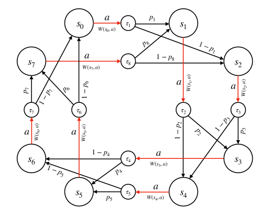
Figure 1: Graphical depiction of a sample MDP

We extend MDP to Weighted MDP (WMDP) by associating a weight to each possible edge. Basically, a WMDP can be observed as a Rewardful MDP, where we gain weights instead of rewards after each action.

Definition 3 (Weighted MDP)

A Weighted MDP (WMDP) is a tuple $\mathcal{M}_{W}=(S,A,T,W)$ where $\mathcal{M}=(S,A,T)$ is an MDP and $W:S\times A\rightarrow\real$ is a function associating a real weight to each state-action pair.

Example 1

Let us graphically illustrate a sample WMDP $\mathcal{M}_{W}$ where $S=\{s_{0},\dots,s_{7}\}$, $A=\{a\}$ and $T(s_{i-1},a)=\tau_{i}\in Dist(S)$ for all $i\in[8]$ where,

$$\tau_{i}(s)=\begin{cases}p_{i}\quad\text{if }i\ (\mathrm{mod}\ 2)=0\text{ and }s=s_{(i+1)\ (\mathrm{mod}\ 8)}\\ 1-p_{i}\quad\text{if }i\ (\mathrm{mod}\ 2)=0\text{ and }s=s_{(i+2)\ (\mathrm{mod}\ 8)}\\ p_{i}\quad\text{if }i\ (\mathrm{mod}\ 2)=1\text{ and }s=s_{i\ (\mathrm{mod}\ 8)}\\ 1-p_{i}\quad\text{if }i\ (\mathrm{mod}\ 2)=1\text{ and }s=s_{(i+1)\ (\mathrm{mod}\ 8)}\\ 0\quad\text{otherwise.}\end{cases}$$

We depict $\mathcal{M}_{W}$ in Figure 1 as a graph where $s_{i}$, $\tau_{j}$ are nodes of the graph, there is a non-deterministic edge from $s_{i}$ to $\tau_{j}$ (marked red) if $T(s_{i},a)=\tau_{j}$ and, there is a probabilistic edge from $\tau_{j}$ to $s_{i}$ if $\tau_{j}(s_{i})\neq 0$. Each non-deterministic edge $(s_{i},\tau_{j})$ is labeled with the action $a$ and the weight of the edge $W(s_{i},a)$. Each probabilistic edge is labeled with its probability.∎

Note that, under a memoryless policy $\rho$, a WMDP not only gives a unique probability, but also gives a unique weight of transition from state $s$ to $s^{\prime}$ (given by $W(s,\rho(s))$). We say a Weighted DTMC (WDTMC) is a WMDP associated with a memoryless policy such that, probability and weight of transition between any two sates are uniquely defined.

The weight of a finite path $\sigma=s_{0},a_{1},s_{1},\dots,s_{n}$ of an WMDP $\mathcal{M}_{W}$, denoted $W(\sigma)$, is the sum of weights of all edges that appear on that path, i.e.,

$$W(\sigma)=\sum_{i=1}^{n}W(s_{i-1},a_{i}).$$

Similarly, Mean payoff of a finite path $\sigma$ is the mean weight of all edges appearing on the finite path.

Definition 4 (Mean Payoff)

For a WMDP $\mathcal{M}_{W}$, the mean payoff $\gamma$ is a function from $\textit{Paths}_{\textit{fin}}(\mathcal{M}_{W})$ to defined as,

$$\gamma(\sigma)=\frac{W(\sigma)}{\left|\sigma\right|}.$$

2.4 Maximum Expected Mean Payoff of WMDP

Given a WMDP, we are interested in finding the maximum expected mean payoff of an infinite path under any policy. Here, we formally state this as a problem and discuss an efficient algorithm for its solution.

Problem 1

Given a WMDP $\mathcal{M}_{W}$, find the maximum expected mean payoff of an infinite path under any policy, i.e.,

$$\sup_{\rho\in\Gamma}\left(\limsup_{n\rightarrow\infty}E^{T^{\rho}_{n}}[\gamma]\right),$$

where $T^{\rho}_{n}$ is a distribution on $\textit{Paths}_{\textit{fin}}(\mathcal{M}_{W})$ given by $T^{\rho}_{n}(\sigma)=T_{\rho}(\sigma\mid\left|\sigma\right|=n)$.

We denote $\limsup_{n\rightarrow\infty}E^{T^{\rho}_{n}}[\gamma]$ as $E_{\rho}[\gamma]$. Now, let us briefly discuss an algorithm for solving the above problem.

2.4.1 Algorithm for calculating maximum expected mean payoff:

Our goal is to solve Problem 1 for a WMDP with finite set of states and actions (finite WMDP). Algorithm 2 (MEC-SI) from [17] solves a similar problem for the class of WMDPs with strictly positive weights and the $\limsup$ in the expected mean payoff replaced with $\liminf$, that is, it computes $\sup_{\rho\in\Gamma}\left(\liminf_{n\rightarrow\infty}E^{T^{\rho}_{n}}[\gamma]\right)$. We want to use this algorithm to solve Problem 1. In order to do that, the input WMDP must be suitably modified to suit the input criterion of Algorithm MEC-SI and, the desired output should be derivable from the output of the algorithm. Note that, $\limsup$ of a real sequence can be found by negating the $\liminf$ of the inverted sequence. Thus, if we negate all weights of the input WMDP and find $\sup_{\rho\in\Gamma}\left(\liminf_{n\rightarrow\infty}E^{T^{\rho}_{n}}[\gamma]\right)$, we are actually finding the maximum expected payoff of the original WMDP. Also, if we shift the outputs of a real valued function by a constant real bias, the expectation gets shifted by the same bias. Thus, solving Problem 1 for a WMDP is the same as solving Problem 1 for the WMDP after shifting each weight by a constant, and then removing the constant. Hence, for a WMDP with both positive and negative weights, we can solve Problem 1 by first negating all the weights, then adding a constant bias to each weight to make them all positive, and finally applying Algorithm MEC-SI on the WMDP with the modified weights.

Let us now briefly describe Algorithm MEC-SI. The main steps of the algorithm are:

1. Achieve Maximal End Component (MEC) decomposition [5] of the input WMDP.

2. For each MEC, find $\sup_{\rho\in\Gamma}\left(\liminf_{n\rightarrow\infty}E^{T^{\rho}_{n}}[\gamma]\right)$ for the induced WMDP by strategy iteration.

3. Construct the MEC-quotient (an MDP) using the values obtained in the previous step [17].

4. Find the maximum reaching probability to a particular state of the MEC-quotient [17].

Note that, the algorithm works in polynomial time [17, 5] if we can solve steps 2 and 4 in polynomial time. Note that, step 2 cannot be done in polynomial time as strategy iteration is not guaranteed to converge in polynomial time. Also note that, we don’t actually need to synthesize an optimal strategy, rather, we only need the optimal gain $\sup_{\rho\in\Gamma}\left(\liminf_{n\rightarrow\infty}E^{T^{\rho}_{n}}[\gamma]\right)$ of the MEC. Let us show how we can do this in polynomial time. If a WMDP is finite and strongly connected (communicating), that is, each state is reachable from every other state, then there is a linear program (LP) formulation for the optimal gain problem [26]. Since MECs are strongly connected [17], we can obtain optimal gain of an MEC by solving an LP. Since an LP can be solved in polynomial time, step 2 can actually be completed in polynomial time as well.

If an MDP is finite, maximum reaching probability to a state can be solved by solving an LP [26]. Since MEC-quotient is a finite MDP [17], we can use this LP formulation for step 4. Thus, step 4 can also be completed in polynomial time. So, we have a polynomial-time algorithm for computing maximum expected mean payoff of a WMDP.

Example 2

Let us apply our algorithm on the sample WMDP described in Example 1. First, we negate each weight, i.e., the modified weight of a state-action pair $(s_{i},a)$ becomes $-W(s_{i},a)$. Now, if $\min_{i\in[8]}(-W(s_{i-1},a))\leq 0$, then we set the constant $c\leftarrow\left|\min_{i\in[8]}(-W(s_{i-1},a))\right|+1$ and $c\leftarrow 0$ otherwise. We add $c$ to each of the modified weights. Thus, the final weight of a state-action pair $(s_{i},a)$ becomes $-W(s_{i},a)+c$, which is strictly positive. We now apply Algorithm MEC-SI on the WMDP with the modified weights. Note that, the WMDP is strongly connected, i.e., it has only one MEC (see [17]). Thus, we can skip steps 3 and 4 altogether. The maximum expected mean payoff of the sample WMDP is simply $-(v-c)$, where $v$ is the value obtained from step 2 by solving the linear program for the WMDP with modified weights.

3 Polyhedral Probabilistic Hybrid Systems

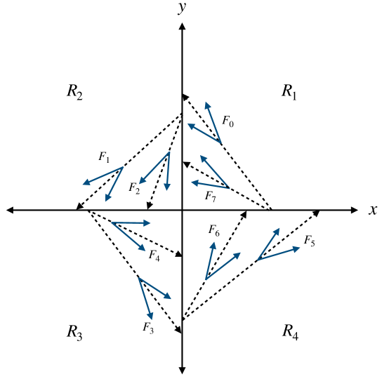
Figure 2: A sample PPHS

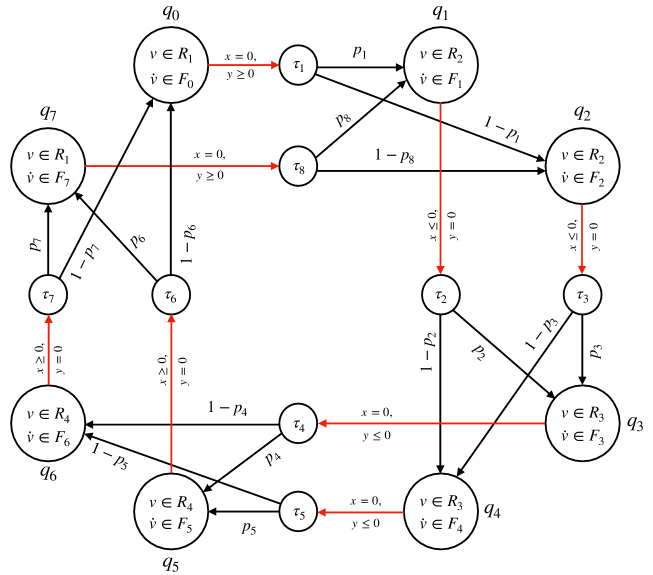
Figure 3: Graphical representation of sample PPHS

In this section, we define Polyhedral Probabilistic Hybrid System (PPHS) and associate a notion of stability to PPHS.

Definition 5 (PPHS)

The Polyhedral Probabilistic Hybrid System (PPHS) is defined as the tuple $\mathcal{H}\coloneqq(Q,\mathcal{X},\textit{I},\textit{F},\textit{E})$ where,

• $Q$ is the set of discrete locations,

• $\mathcal{X}={}^{n}$ is the continuous state space for some $n\in\mathbb{N}$,

• $\textit{I}:Q\rightarrow Poly(n)$ is the invariant function which assigns a positive scaling invariant polyhedral subset of the state space to each location $q\in Q$,

• $\textit{F}:Q\rightarrow Poly(n)$ is the Flow function which associates a flow polyhedron to each location $q\in Q$

• $\textit{E}\subseteq Q\times(\cup_{q\in Q}\mathbb{F}(\textit{I}(q)))\times Dist(Q)$ is the probabilistic edge relation such that $(q,f,\zeta)\in\textit{E}$ where for every $(q,f)$, there is a at most one $\zeta$ such that $(q,f,\zeta)\in\textit{E}$ and $f\in\mathbb{F}(\textit{I}(q))$. $f$ is called a Guard of the location $q$.

Let us describe the semantics of the PPHS. An execution starts from $(q_{0},x_{0})$ where $q_{0}\in Q$ and $x_{0}\in\textit{I}(q_{0})$. It evolves continuously for some time $T$ according to a flow rate that is chosen non-deterministically from $\textit{F}(q_{0})$, until it reaches a facet $f_{0}$ of $\textit{I}(q_{0})$. Then a probabilistic discrete transition is taken if there is an edge $(q_{0},f_{0},\zeta_{0})$ and the state $q_{0}$ is probabilistically changed to $q_{1}$ with probability $\zeta_{0}(q_{1})$. The execution (tree) continues with alternating continuous and discrete transitions.

Formally, for $x_{1},x_{2}\in\mathcal{X}$ and $q\in Q$, we say that there is a continuous transition from $x_{1}$ to $x_{2}$ with respect to $q$ if $x_{1},x_{2}\in\textit{I}(q)$, there exists $R\geq 0$ and $f\in\textit{F}(q)$ such that $x_{2}=x_{1}+f\cdot R$, $x_{1}+\textit{F}(q)\cdot t\in\textit{I}(q)$ for all $0\leq t<R$ and $x_{2}\in\partial(\textit{I}(q))$. If for all $t\geq 0$, $x_{1}+\textit{F}(q)\cdot t\in\textit{I}(q)$ then we say $x_{1}$ has an infinite edge with respect to $q$. For two locations $q_{1},q_{2}\in Q$, we say there is a discrete transition from $q_{1}$ to $q_{2}$ with probability $p$ via $\zeta\in Dist(Q)$ and $f\in\mathbb{F}(q_{1})$ if $f\subseteq\textit{I}(q_{2})$, $(q_{1},f,\zeta)\in\textit{E}$ and $p=\zeta(q_{2})$.

Example 3

Let us illustrate PPHS using an example. Let $\{q_{i-1}\mid i\in[8]\}$ be the set of discrete locations and $\mathcal{X}={}^{2}$ be the continuous state space for a PPHS $\mathcal{H}$. The four quadrants $R_{1}$, $R_{2}$, $R_{3}$ and $R_{4}$ are the invariant regions with $R_{1}$ associated to $q_{0}$ and $q_{7}$, $R_{2}$ associated to $q_{1}$ and $q_{2}$, $R_{3}$ associated to $q_{3}$ and $q_{4}$ and, $R_{4}$ associated to $q_{5}$ and $q_{6}$. The rate of change of continuous state (flow rate) at location $q_{i}$ is non-deterministically chosen from the polyhedron $F_{i}\subseteq{}^{2}$. For each location, either positive $X$, or positive $Y$, or negative $X$, or negative $Y$ axis serves as the guard, that is, the system probabilistically jumps to a new location once the continuous state reaches the guard. For example, if the continuous state of the system becomes $(0,y)$ for some $y\in\real$ when the system is in $q_{0}$, then the system will change its location to either $q_{1}$ or $q_{2}$ probabilistically, since positive $Y$ axis is the guard of $q_{0}$. We illustrate the possible evolutions of the system in Figure 2.

We also provide a graphical depiction of the PPHS in Figure 3. Note that, each location $q_{i}$ is labeled with $v\in R_{j},\dot{v}\in F_{i}$, which implies that the continuous state $v$ belongs to the the invariant $R_{j}$ and rate of change of the continuous state $\dot{v}$ belongs to the flow polyhedron $F_{i}$ associated to the location. Each non-deterministic edge outgoing from a location $q_{i}$ (marked red) is labeled with a guard set and leads to a probability distribution $\tau_{i+1}$ on $Q$. Probabilistic edges are directed from $\tau_{i}$ to the next possible locations and labeled with the probability of the target location under $\tau_{i}$.∎

We capture the semantics of a PPHS using a WMDP, where continuous transitions are analogous to non-deterministic actions and discrete transitions are equivalent to probabilistic change of state. To reason about convergence, we need to capture the relative distance of the states from the equilibrium point, which is captured using edge weights. Let us fix $0$ as the equilibrium point for the rest of the section. The weight on a transition from $(q_{1},x_{1})$ to $(q_{2},x_{2})$ captures the logarithm of the relative distance of $x_{1}$ and $x_{2}$ from $0$, that is, $\log\left(\lvert\!\lvert x_{2}\rvert\!\rvert/\lvert\!\lvert x_{1}\rvert\!\rvert\right)$, where $\lvert\!\lvert x\rvert\!\rvert$ captures the distance of state $x$ from $0$.

Definition 6 (Semantics of PPHS)

Given a PPHS $\mathcal{H}$, we can construct the WMDP ${\llbracket\mathcal{H}\rrbracket}\coloneqq(S_{\mathcal{H}},A_{\mathcal{H}},T_{\mathcal{H}},W_{\mathcal{H}})$ where,

• $S_{\mathcal{H}}=Q\times\mathcal{X}$

• $A_{\mathcal{H}}\subseteq S_{\mathcal{H}}\times S_{\mathcal{H}}$ with $((q_{1},x_{1}),(q_{2},x_{2}))\in A$ iff $q_{1}=q_{2}$ and there is a continuous transition from $x_{1}$ to $x_{2}$ with respect to $q_{1}$.

• $T_{\mathcal{H}}((q_{2},x_{2})|(q_{1},x_{1}),a)=\zeta(q_{2})=p$ if $a=((q_{1},x_{1}),(q_{1},x_{2}))$, there is a discrete transition from $q_{1}$ to $q_{2}$ with probability $p$ via $\zeta$ and $f$, and $x_{2}\in f$. In all other cases, $T_{\mathcal{H}}((q_{2},x_{2})|(q_{1},x_{1}),a)=0$.

• $W_{\mathcal{H}}((q_{1},x_{1}),a)=\log\left(\lvert\!\lvert x_{2}\rvert\!\rvert/\lvert\!\lvert x_{1}\rvert\!\rvert\right)$ where $a=((q_{1},x_{1}),(q_{1},x_{2}))$.

An infinite path $\sigma=(q_{0},x_{0}),((q_{0},x_{0}),(q_{0},x_{1})),(q_{1},x_{1}),\dots$ of the semantics WMDP ${\llbracket\mathcal{H}\rrbracket}$ is said to converge to $0$ if $\lim_{n\rightarrow\infty}\lvert\!\lvert x_{n}\rvert\!\rvert=0$. Thus, $\sigma$ converges if and only if $W_{\mathcal{H}}(\sigma)=-\infty$, if and only if $\limsup_{n\rightarrow\infty}\frac{W_{\mathcal{H}}(\sigma[0:n])}{n}<0$ [9]. Thus, $\sigma$ converges if and only if mean payoff of $\sigma$ is less than zero. We say a WMDP is stable if an infinite path of it converges in expectation under any policy. A PPHS is said to be stable when its semantics WMDP is stable.

Definition 7 (Stability of PPHS)

A WMDP $\mathcal{M}_{W}$ is said to be stable if under any policy $\rho$, an infinite path of it converges in expectation, i.e., $E_{\rho}[\gamma]<0$. A PPHS $\mathcal{H}$ is said to be stable when its semantics WMDP ${\llbracket\mathcal{H}\rrbracket}$ is stable.

For a WMDP, an infinite path converges in expectation under all policies, if and only if, maximum expected mean payoff of an infinite path is less than zero. Thus, we have the following characterization for stability of a PPHS,

Theorem 3.1

[Characterization of Stability] A PPHS $\mathcal{H}$ is stable iff, maximum expected mean payoff of an infinite path of its semantics WMDP ${\llbracket\mathcal{H}\rrbracket}$ is strictly negative, i.e.,

$$\sup_{\rho\in\Gamma}E_{\rho}[\gamma]<0.$$

Proof

A PPHS $\mathcal{H}$ is stable when its semantics WMDP ${\llbracket\mathcal{H}\rrbracket}$ is stable. Now, ${\llbracket\mathcal{H}\rrbracket}$ is stable if and only if $E_{\rho}[\gamma]<0$ $\forall\rho\in\Gamma$, if and only if $\sup_{\rho\in\Gamma}E_{\rho}[\gamma]<0$. Hence, our claim is proved.∎

However, the algorithm discussed in Section 2.4.1 cannot be applied to ${\llbracket\mathcal{H}\rrbracket}$ since it has infinite state and action space. Hence, we create an abstract WMDP $\mathcal{H}^{\text{red}}$ from ${\llbracket\mathcal{H}\rrbracket}$ which is finite in size and, stability of $\mathcal{H}^{\text{red}}$ implies stability of ${\llbracket\mathcal{H}\rrbracket}$.

Remark 1

Different notions of stability, such as, exponential stability, Lyapunov stability, Lagrange stability, asymptotic stability, have been explored for non-probabilistic hybrid systems. These notions have been extended for SHS [29] by defining them on expected behavior of the system. For example, an SHS is said to be Lyapunov stable around a point of equilibrium when the system remains within a close neighborhood of the equilibrium point in the expected case, when it starts from a point close to the equilibrium point. We can say that, our notion of stability extends the notion of asymptotic stability in the non-stochastic setting, since we obtain the definition of asymptotic stability in non-stochastic setting by removing the ‘in expectation’ part from Definition 7.

4 Abstraction of PPHS to WMDP

We now describe the abstract WMDP $\mathcal{H}^{\text{red}}$ derived from the semantics WMDP ${\llbracket\mathcal{H}\rrbracket}$ of a PPHS $\mathcal{H}$, and show that, stability of $\mathcal{H}^{\text{red}}$ implies stability of ${\llbracket\mathcal{H}\rrbracket}$.

Definition 8 (Abstract WMDP)

Let $\mathcal{H}$ be a PPHS and ${\llbracket\mathcal{H}\rrbracket}$ be its semantics. We define the WMDP $\mathcal{H}^{\text{red}}=(S^{\text{red}},A^{\text{red}},T^{\text{red}},W^{\text{red}})$ as follows,

• $S^{\text{red}}=Q\times\bigcup_{q\in Q}\mathbb{F}(\textit{I}(q))$

• $A^{\text{red}}\subseteq S^{\text{red}}\times S^{\text{red}}$ with $((q_{1},f_{1}),(q_{2},f_{2}))\in A$ iff $q_{1}=q_{2}$ and there is a continuous transition from $x_{1}\in f_{1}$ to $x_{2}\in f_{2}$ with respect to $q_{1}$.

• $T^{\text{red}}((q_{2},f_{2})|(q_{1},f_{1}),a)=T_{\mathcal{H}}((q_{2},x_{2})|(q_{1},x_{1}),a^{\prime})$ if $a=((q_{1},f_{1}),(q_{1},f_{2}))$, $x_{1}\in f_{1}$, $x_{2}\in f_{2}$ and $T_{\mathcal{H}}((q_{2},x_{2})|(q_{1},x_{1}),a^{\prime})>0$. In all other cases, $T^{\text{red}}((q_{2},f_{2})|(q_{1},f_{1}),a)=0$.

• $W^{\text{red}}((q_{1},f_{1}),((q_{1},f_{1}),(q_{1},f_{2})))=\max\{W_{\mathcal{H}}((q_{1},x_{1}),a^{\prime})\}$, where maximum is taken over all $a^{\prime}$ of the form $((q_{1},x_{1}),(q_{2},x_{2}))$ such that $x_{1}\in f_{1}$ and $x_{2}\in f_{2}$.

Note that, $\mathcal{H}^{\text{red}}$ has finite state space and action space since for any $q\in Q$, $\mathbb{F}(\textit{I}(q))$ is finite. Also, $\max\{W_{\mathcal{H}}((q_{1},x_{1}),a^{\prime},(q_{2},x_{2}))\}$, where maximum is taken over all $((q_{1},x_{1}),a^{\prime},(q_{2},x_{2}))\in\mathcal{E}_{\mathcal{H}}$ such that $x_{1}\in f_{1}$ and $x_{2}\in f_{2}$, can be calculated by solving linear optimization problems when $\textit{I}(q_{1})$ is positive scaling invariant (see [22]).

Example 4

For example, let us abstract the PPHS described in Example 3. Assuming $(1,0)$ to be the initial state and $q_{0}$ the initial location, $(q_{0},\{x\geq 0,y=0\})$ gives the initialization point for the abstract WMDP. A unique action $((q_{0},\{x\geq 0,y=0\}),(q_{0},\{x=0,y\geq 0\}))$ leads from the initialization point to the distribution $\tau_{1}$ with non-zero weight. $\tau_{1}$ has probability $p_{1}$ for state $(q_{1},\{x=0,y\geq 0\})$ and probability $1-p_{1}$ for state $(q_{2},\{x=0,y\geq 0\})$. Other states and transitions are defined similarly. The resulting WMDP is depicted by Figure 1, where $s_{0}$ marks the initialization point.∎

We will now prove that $\mathcal{H}$ is stable if $\mathcal{H}^{\text{red}}$ is stable. This result will lead to a polynomial time algorithm that can verify stability of PPHS.

Theorem 4.1

$\mathcal{H}$ is stable if $\mathcal{H}^{\text{red}}$ is stable.

Proof

Let $\rho$ be an arbitrary policy of ${\llbracket\mathcal{H}\rrbracket}$. Suppose, $(q_{0},x_{0})$ is the initialization point of ${\llbracket\mathcal{H}\rrbracket}$ and $x_{0}$ belongs to the facet $f_{0}$. Then, $(q_{0},f_{0})$ is the initialization point of $\mathcal{H}^{\text{red}}$. We say that a state $(q,x)$ of ${\llbracket\mathcal{H}\rrbracket}$ belongs to a state $(q^{\prime},f^{\prime})$ of $\mathcal{H}^{\text{red}}$, denoted as $(q,x)\in(q^{\prime},f^{\prime})$, if $q=q^{\prime}$ and $x\in f^{\prime}$. We define a policy $\hat{\rho}$ for $\mathcal{H}^{\text{red}}$ using $\rho$ as follows:

• Let $\hat{\sigma}=(q_{0},f_{0}),((q_{0},f_{0}),(q_{0},f_{1})),(q_{1},f_{1}),\dots,(q_{n},f_{n})$ be a finite path of $\mathcal{H}^{\text{red}}$ and the action $((q_{n},f_{n}),(q_{n},f^{\prime}))$ $\in A^{\text{red}}$.

• Then,

  $$\hat{\rho}(\hat{\sigma})=((q_{n},f_{n}),(q_{n},f^{\prime}))$$

  $$\text{iff, }\exists\sigma\in\textit{Paths}_{\textit{fin}}({\llbracket\mathcal{H}\rrbracket}),\sigma_{i}\in\hat{\sigma}_{i}\quad\forall i\in[n],\text{ and }x^{\prime}\in f^{\prime},$$

  where $\rho(\sigma)=((q_{n},x_{n}),(q_{n},x^{\prime}))$.

This implies by construction of $\mathcal{H}^{\text{red}}$ that, probability of a finite path $\hat{\sigma}$ under policy $\hat{\rho}$ is simply the probability (under $\rho$) of set of all finite paths $\sigma$ of ${\llbracket\mathcal{H}\rrbracket}$ such that $\left|\hat{\sigma}\right|=\left|\sigma\right|$ and $\sigma_{i}\in\hat{\sigma}_{i}$ for all $i$. Also note that, $W^{\text{red}}(\hat{\sigma})\geq W_{\mathcal{H}}(\sigma)$ for any such $\sigma\in\textit{Paths}_{\textit{fin}}({\llbracket\mathcal{H}\rrbracket})$. In fact, for $\hat{\sigma}\in\textit{Paths}_{\textit{fin}}(\mathcal{H}^{\text{red}})$, let

$$\Pi(\hat{\sigma})=\{\sigma\in\textit{Paths}_{\textit{fin}}({\llbracket\mathcal{H}\rrbracket}):\sigma_{i}\in\hat{\sigma}_{i}\text{ }\forall i\};$$

then, for each $\sigma\in\Pi(\hat{\sigma})$,

$$\frac{W_{\mathcal{H}}(\sigma)}{\left|\sigma\right|}\leq\frac{W^{\text{red}}(\hat{\sigma})}{\left|\hat{\sigma}\right|}\text{ and,}$$

$$T_{\hat{\rho}}(\hat{\sigma})=T_{\rho}\left(\Pi(\hat{\sigma})\right)\quad\text{for all }\hat{\sigma}\in\textit{Paths}_{\textit{fin}}(\mathcal{H}^{\text{red}}).$$

Since for any $\sigma\in\textit{Paths}_{\textit{fin}}({\llbracket\mathcal{H}\rrbracket})$, there exists $\hat{\sigma}\in\textit{Paths}_{\textit{fin}}(\mathcal{H}^{\text{red}})$ such that $\left|\sigma\right|=\left|\hat{\sigma}\right|$ and $\sigma_{i}\in\hat{\sigma}_{i}$ for all $i$,

$$\bigcup_{\hat{\sigma}\in\textit{Paths}_{\textit{fin}}(\mathcal{H}^{\text{red}})}\Pi(\hat{\sigma})=\textit{Paths}_{\textit{fin}}({\llbracket\mathcal{H}\rrbracket}).$$

Thus, expected mean payoff of an infinite path of $\mathcal{H}^{\text{red}}$ under $\hat{\rho}$,

$$E_{\hat{\rho}}[\gamma]= \limsup_{n\rightarrow\infty}\sum_{\hat{\sigma}\in\textit{Paths}_{\textit{fin}}(\mathcal{H}^{\text{red}})}\left(\frac{W^{\text{red}}(\hat{\sigma})}{\left|\hat{\sigma}\right|}\right)T_{n}^{\hat{\rho}}(\hat{\sigma})$$

$$= \limsup_{n\rightarrow\infty}\sum_{\hat{\sigma}\in\textit{Paths}_{\textit{fin}}(\mathcal{H}^{\text{red}})}\left(\frac{W^{\text{red}}(\hat{\sigma})}{\left|\hat{\sigma}\right|}\right)T_{n}^{\rho}(\Pi(\hat{\sigma}))$$

$$\geq \limsup_{n\rightarrow\infty}\sum_{\sigma\in\textit{Paths}_{\textit{fin}}({\llbracket\mathcal{H}\rrbracket})}\left(\frac{W_{\mathcal{H}}(\sigma)}{\left|\sigma\right|}\right)T_{n}^{\rho}(\sigma)=E_{\rho}[\gamma],$$

that is, expected mean payoff of an infinite path of ${\llbracket\mathcal{H}\rrbracket}$ under $\rho$. Since for any arbitrary policy $\rho$ of ${\llbracket\mathcal{H}\rrbracket}$, we can define a policy $\hat{\rho}$ of $\mathcal{H}^{\text{red}}$ such that $E_{\hat{\rho}}[\gamma]\geq E_{\rho}[\gamma]$, we can say that,

$$\sup_{\hat{\rho}\in\Gamma_{\mathcal{H}^{\text{red}}}}E[\gamma]\geq\sup_{\rho\in\Gamma_{{\llbracket\mathcal{H}\rrbracket}}}E[\gamma].$$

Thus, stability of $\mathcal{H}^{\text{red}}$, i.e., $E_{\hat{\rho}}[\gamma]<0$ for all $\hat{\rho}\in\Gamma_{\mathcal{H}^{\text{red}}}$, implies $\sup_{\hat{\rho}\in\Gamma_{\mathcal{H}^{\text{red}}}}E_{\hat{\rho}}[\gamma]<0$, which further implies $\sup_{\rho\in\Gamma_{{\llbracket\mathcal{H}\rrbracket}}}E_{\rho}[\gamma]<0$, which, by Theorem 3.1 implies that $\mathcal{H}$ is stable too. Hence, our claim is proved.∎

Using Theorem 4.1, we can easily device a polynomial time algorithm that can verify stability of a PPHS $\mathcal{H}$. We simply construct $\mathcal{H}^{\text{red}}$ from ${\llbracket\mathcal{H}\rrbracket}$, which takes polynomial time according to [22], and apply the polynomial time algorithm discussed in Section 2.4.1 on $\mathcal{H}^{\text{red}}$ to find the maximum expected mean payoff of an infinite path of $\mathcal{H}^{\text{red}}$. If the maximum expected mean payoff is less than zero, then we deduce that $\mathcal{H}$ is stable. Note that, our algorithm tests a sufficient condition for stability, i.e., we cannot say that the PPHS is unstable if the algorithm does not guarantee stability.

Remark 2

We would like to remark on the generality of this abstraction procedure. Note that, Theorem 4.1 holds even if we define stability using a different payoff function, like total effective payoff [2] or, prefix-independent and submixing payoff [13]. Not only that, it works for other notions of stability as well, such as almost sure stability. However, the algorithm for verifying stability of the abstract WMDP (Section 2.4.1) is not so general and needs to be modified for different notions of stability.

5 Experimental Evaluation

$n$	Expt No.	Locs	$\left|\mathcal{E}_{\mathcal{M}_{W}}\right|$	Time (sec)		Stability
				$T^{\text{red}}$	$T^{\text{stab}}$
$2$	1	$4$	$16$	$0.113$	$1.8\times 10^{-4}$	Unknown
	2	$8$	$64$	$0.242$	$0.143$	Yes
	3	$12$	$144$	$0.367$	$0.149$	Yes
	4	$16$	$256$	$0.517$	$0.158$	Yes
$3$	1	$8$	$48$	$3.042$	$7.3\times 10^{-4}$	Unknown
	2	$16$	$192$	$6.059$	$0.213$	Yes
	3	$24$	$432$	$9.203$	$0.311$	Yes
	4	$32$	$768$	$12.213$	$0.438$	Yes
$4$	1	$4$	$24$	$2.676$	$5\times 10^{-4}$	Unknown
	2	$8$	$96$	$5.784$	$0.163$	Yes
	3	$12$	$216$	$9.018$	$0.197$	Yes
	4	$16$	$384$	$11.678$	$0.244$	Yes
$5$	1	$10$	$90$	$11.986$	$1.4\times 10^{-3}$	Unknown
	2	$20$	$360$	$25.098$	$0.275$	Yes
	3	$30$	$810$	$37.356$	$0.438$	Yes
	4	$40$	$1440$	$49.743$	$0.67$	Yes
$6$	1	$20$	$240$	$38.377$	$4\times 10^{-3}$	Unknown
	2	$40$	$960$	$78.049$	$0.631$	Yes
	3	$60$	$2160$	$120.906$	$1.241$	Yes
	4	$80$	$3840$	$160.049$	$2.08$	Yes

Table 1: Verification of stability of PPHS

In this section, we provide a brief overview of our implementation of the abstraction based stability verification algorithm of PPHS and test it on a set of PPHS benchmarks. Recall that, our technique consists of abstraction of a PPHS to a finite WMDP and verification of stability of the abstract WMDP using the algorithm developed in Section 2.4.1. We have implemented the abstraction procedure and the algorithm using Python. The abstract WMDP is stored as annotated graph using the networkx [14] package. In order to calculate each edge weight, $4n^{2}$ linear programming problems has to be solved, where $n$ is the number of dimensions [22]. This has been done using the pplpy package. To find all MECs of the WMDP through strongly connected component decomposition [5], networkx functions are used. For linear programming, the software Gurobi and its python handler gurobipy are used. All experiments have been performed on macOS Big Sur with Quad-Core (Intel Core i7) $2.8\text{GHz}\times 1$ Processor and 16GB RAM.

We have tested the effect of increasing the number of dimensions and the number of locations of the PPHS on the time requirement of our algorithm. We have varied the number of dimensions $n$ from $2$ to $6$ and created four sample PPHS for each dimension. For dimension $2$ and $3$, four quadrants of ² and eight octants of ³ are chosen respectively as the invariant regions. For higher dimensions ($n=4$, $5$ and $6$), $3$-dimensional hyperplanes of ⁿ are chosen as the invariant regions. For experiment $j$ ($j\in[4]$) of dimension $n$, $j$ locations are created for each invariant region. For example, the PPHS corresponding to experiment $2$ of dimension $3$ has $2$ locations per octant, i.e., $2\times 8=16$ locations in total. For experiment $1$ in all dimensions, the flow polyhedron is set for each location such that at least one edge of the abstract WMDP has infinite weight. For experiments $3$ and $4$, flows are set such that at least one edge of the WMDP has positive weight. For experiment $2$ however, all flows are set such that no edge of the abstract WMDP can have positive weight.

We present our findings in Table 1. Here $n$ is number of dimensions, Locs is the total number of locations of the PPHS corresponding to the experiment, $\left|\mathcal{E}_{\mathcal{M}_{W}}\right|$ is the number of edges of the abstract WMDP, $T^{\text{red}}$ denotes the time taken to generate the abstract WMDP and $T^{\text{stab}}$ denotes the time taken to verify stability of the abstract WMDP. For each experiment, the average time over $50$ runs is reported. Finally, the Stability column provides the information on whether the PPHS is stable or not. Note that, a PPHS is stable if the abstract WMDP is stable, not necessarily the other way round. Thus, we cannot say a PPHS is unstable if the stability checking algorithm (Section 2.4.1) designates the abstract WMDP to be unstable. Hence, in such cases, we have reported “Unknown” in the Stability column. In other cases, we have reported “Yes” in the Stability column, which means that the corresponding PPHS is found to be stable. We observe that the abstraction time dominates over the verification time in all cases. In fact, the abstraction time increases rapidly with the number of dimensions $n$. This is expected since calculation of each edge weight of the abstract WMDP requires solving $4n^{2}$ linear programs [22]. Increase in the number of locations results in increased abstraction time as well since number of edges of the abstract WMDP increases. The verification time however, does not always increase with the number of dimensions. This is because, the verification time depends on the number of edges of the abstract WMDP and not on the number of dimensions. For experiment $1$ however, verification time is extremely small as the algorithm has found an infinite weighted edge and deduces the abstract WMDP to be unstable without going through MEC-decomposition or LP solving.

For our second set of experiments, we test our algorithm on Linear Switched Systems [25]. For Linear Switched System with ⁿ as the continuous state space, rate of change of the continuous state $v$ is a linear function of the current state, and this linear function changes arbitrarily. More precisely, the system evolving with dynamics $\dot{v}=A_{1}v$ ($A_{1}\in{}^{n\times n}$) can change its dynamics to $\dot{v}=A_{2}v$ (${}^{n\times n}\ni A_{2}\neq A_{1}$) arbitrarily. We take Example 2 from [25] where the system evolves in ² with dynamics $\dot{v}=Av$, and $A$ switches between

$$A_{1}=\begin{bmatrix}-5&\quad-4\\ -1&\quad-2\end{bmatrix}\text{ and }A_{2}=\begin{bmatrix}-2&\quad-4\\ 20&\quad-2\end{bmatrix}.$$

Instead of arbitrary switching, we assume probabilistic switching of dynamics, i.e., at any point of time the system either retains its dynamics or changes it (if possible) with equal probability. To analyze stability of this system, we apply hybridization technique discussed in [21]. Basically, we partition the continuous state space into positively scaled regions and associate two locations to each partition such that, for the $i^{th}$ location, dynamics is given by $\dot{v}\in F_{i}$ ($F_{i}$ is the polyhedron formed by points $A_{i}v$, where $v$ belongs to the partition). Change of location is allowed at the boundary of the corresponding partition only, at which point, one of the locations from the adjacent partition is chosen with equal probability. Clearly, this process generates a PPHS. We analyze stability of the PPHS using our algorithm and generate PPHS with finer partitions until stability is ensured. Note that, stability of the PPHS implies stability of the Linear Switched System [21]. In fact, we used the same partitions as in test cases SS4_1, SS8_1 and SS16_1 of [21]. Stability is ensured for both PPHS corresponding to SS8_1 and SS16_1 and not for the PPHS corresponding to SS4_1, which matches with the observations of [21].

6 Conclusion

In this paper, we have presented an algorithm for stability analysis of an important subclass of Stochastic Hybrid Systems, which we call the Polyhedral Probabilistic Hybrid System (PPHS). Our algorithm is based on abstraction based techniques, where we first abstract the PPHS to a finite WMDP and then test the abstract WMDP for stability. Verification of stability of the abstract WMDP is extremely efficient, since it can be done using a polynomial-time algorithm. However, the abstraction time increases rapidly with the number of dimensions and always dominates over the verification time. Hence, the entire process suffers from the curse of dimensionality. For our future work, we would like to develop compositional methods for analyzing stochastic stability to circumvent this problem. Two other directions of future research are, exploring probabilistic stability analysis for almost sure notions and for more complex dynamics, including those with stochasticity in the continous dynamics and, analyzing stability in a chosen set of dimensions instead of all the dimensions, which is hard to achieve in reality.

References

- [1] Alur, R., Dang, T., Ivančić, F.: Counter-example guided predicate abstraction of hybrid systems. In: International Conference on Tools and Algorithms for the Construction and Analysis of Systems. pp. 208–223. Springer (2003)
- [2] Boros, E., Elbassioni, K., Gurvich, V., Makino, K.: Markov decision processes and stochastic games with total effective payoff. Annals of Operations Research pp. 1–29 (2018)
- [3] Branicky, M.: Multiple lyapunov functions and other analysis tools for switched and hybrid systems. IEEE Transactions on Automatic Control 43(4), 475–482 (1998). https://doi.org/10.1109/9.664150
- [4] Chatterjee, K., Doyen, L.: Games and markov decision processes with mean-payoff parity and energy parity objectives. In: Mathematical and Engineering Methods in Computer Science: 7th International Doctoral Workshop, MEMICS 2011, Lednice, Czech Republic, October 14-16, 2011, Revised Selected Papers 7. pp. 37–46. Springer (2012)
- [5] Chatterjee, K., Łacki, J.: Faster algorithms for markov decision processes with low treewidth. In: Computer Aided Verification: 25th International Conference, CAV 2013, Saint Petersburg, Russia, July 13-19, 2013. Proceedings 25. pp. 543–558. Springer (2013)
- [6] Cheng, P., Deng, F.: Almost sure exponential stability of linear impulsive stochastic differential systems. In: Proceedings of the 31st Chinese Control Conference. pp. 1553–1557. IEEE (2012)
- [7] Cheng, P., Deng, F., Yao, F.: Almost sure exponential stability and stochastic stabilization of stochastic differential systems with impulsive effects. Nonlinear Analysis: Hybrid Systems 30, 106–117 (2018)
- [8] Clarke, E., Fehnker, A., Han, Z., Krogh, B., Ouaknine, J., Stursberg, O., Theobald, M.: Abstraction and counterexample-guided refinement in model checking of hybrid systems. International journal of foundations of computer science 14(04), 583–604 (2003)
- [9] Das, S., Prabhakar, P.: Stability analysis of planar probabilistic piecewise constant derivative systems. In: International Conference on Quantitative Evaluation of Systems. pp. 192–213. Springer (2022)
- [10] Davrazos, G., Koussoulas, N.: A review of stability results for switched and hybrid systems. In: Mediterranean Conference on Control and Automation. Citeseer (2001)
- [11] Do, K.D., Nguyen, H.: Almost sure exponential stability of dynamical systems driven by lévy processes and its application to control design for magnetic bearings. International Journal of Control 93(3), 599–610 (2020)
- [12] Giesl, P., Hafstein, S.: Review on computational methods for lyapunov functions. Discrete & Continuous Dynamical Systems-B 20(8), 2291 (2015)
- [13] Gimbert, H.: Pure stationary optimal strategies in markov decision processes. In: Annual Symposium on Theoretical Aspects of Computer Science. pp. 200–211. Springer (2007)
- [14] Hagberg, A.A., Schult, D.A., Swart, P.J.: Exploring network structure, dynamics, and function using networkx. In: Varoquaux, G., Vaught, T., Millman, J. (eds.) Proceedings of the 7th Python in Science Conference. pp. 11 – 15. Pasadena, CA USA (2008)
- [15] Hu, L., Mao, X.: Almost sure exponential stabilisation of stochastic systems by state-feedback control. Automatica 44(2), 465–471 (2008)
- [16] Kozin, F.: A survey of stability of stochastic systems. Automatica 5(1), 95–112 (1969)
- [17] Křetínskỳ, J., Meggendorfer, T.: Efficient strategy iteration for mean payoff in markov decision processes. In: Automated Technology for Verification and Analysis: 15th International Symposium, ATVA 2017, Pune, India, October 3–6, 2017, Proceedings. pp. 380–399. Springer (2017)
- [18] Lal, R., Prabhakar, P.: Hierarchical abstractions for reachability analysis of probabilistic hybrid systems. In: 2018 56th Annual Allerton Conference on Communication, Control, and Computing (Allerton). pp. 848–855. IEEE (2018)
- [19] Lal, R., Prabhakar, P.: Counterexample guided abstraction refinement for polyhedral probabilistic hybrid systems. ACM Transactions on Embedded Computing Systems (TECS) 18(5s), 1–23 (2019)
- [20] Liberzon, D.: Switching in systems and control. Springer Science & Business Media (2003)
- [21] Prabhakar, P., García Soto, M.: Hybridization for stability analysis of switched linear systems. In: Proceedings of the 19th International Conference on Hybrid Systems: Computation and Control. pp. 71–80 (2016)
- [22] Prabhakar, P., Soto, M.G.: Abstraction based model-checking of stability of hybrid systems. In: International Conference on Computer Aided Verification. pp. 280–295. Springer (2013)
- [23] Prabhakar, P., Viswanathan, M.: On the decidability of stability of hybrid systems. In: Proceedings of the 16th international conference on Hybrid systems: computation and control. pp. 53–62 (2013)
- [24] Prajna, S., Jadbabaie, A.: Safety verification of hybrid systems using barrier certificates. In: International Workshop on Hybrid Systems: Computation and Control. pp. 477–492. Springer (2004)
- [25] Prajna, S., Papachristodoulou, A.: Analysis of switched and hybrid systems-beyond piecewise quadratic methods. In: Proceedings of the 2003 American Control Conference, 2003. vol. 4, pp. 2779–2784. IEEE (2003)
- [26] Puterman, M.L.: Markov decision processes: discrete stochastic dynamic programming. John Wiley & Sons (2014)
- [27] Rutten, J.J., Kwiatkowska, M., Norman, G., Parker, D.: Mathematical techniques for analyzing concurrent and probabilistic systems. No. 23, American Mathematical Soc. (2004)
- [28] Singh, S.P.: Reinforcement learning algorithms for average-payoff markovian decision processes. In: AAAI. vol. 94, pp. 700–705 (1994)
- [29] Teel, A.R., Subbaraman, A., Sferlazza, A.: Stability analysis for stochastic hybrid systems: A survey. Automatica 50(10), 2435–2456 (2014)
- [30] Van Der Schaft, A.J., Schumacher, J.M.: An introduction to hybrid dynamical systems, vol. 251. Springer London (2000)
- [31] Verdejo, H., Vargas, L., Kliemann, W.: Stability of linear stochastic systems via lyapunov exponents and applications to power systems. Applied Mathematics and Computation 218(22), 11021–11032 (2012)
- [32] Wang, B., Zhu, Q.: Asymptotic stability in distribution of stochastic systems with semi-markovian switching. International Journal of Control 92(6), 1314–1324 (2019)
- [33] Yuan, C., Mao, X.: Asymptotic stability in distribution of stochastic differential equations with markovian switching. Stochastic processes and their applications 103(2), 277–291 (2003)
- [34] Zhang, H., Wu, Z., Xia, Y.: Exponential stability of stochastic systems with hysteresis switching. Automatica 50(2), 599–606 (2014)