Imprints of a Supercooled Phase Transition in the Gravitational
Wave Spectrum from a Cosmic String network

Abstract

A network of cosmic strings (CS), if present, would continue emitting gravitational waves (GW) as it evolves throughout the history of the Universe. This results in a characteristic broad spectrum making it a perfect source to infer the expansion history. In particular, a short inflationary period caused by a supercooled phase transition would cause a drop in the spectrum at frequencies corresponding to that event. However, the impact on the spectrum is similar to the ones caused by an early matter-dominated era or from particle production, making it difficult to disentangle these different physical origins. We point out that, in the case of a short inflationary period, the GW spectrum receives an additional contribution from the phase transition itself. This leads to a characteristic imprint of a peak on top of a wide plateau both visible at future GW observatories.

I Introduction

Both the Standard Model of Particle Physics (SM) and the Standard $\Lambda$CDM Cosmological Model describe with remarkable accuracy a vast amount of observational data on the fundamental interactions of elementary particles ParticleDataGroup:2022pth and on the dynamics and composition of the Universe Planck:2018vyg . Nevertheless, given the large number of unexplained free parameters, this framework is better viewed as an effective description, one that is incomplete at the fundamental level. For instance, explaining the matter-antimatter asymmetry or the nature of the dark matter requires extending the SM, possibly with new particles featuring additional interactions. These additional degrees of freedom might induce deviations from the standard early universe evolution Allahverdi:2020bys . Well known examples are an early matter dominated period before the universe became radiation dominated, or a kination era when the background equation-of-state is more stiff than that of radiation Peebles:1998qn ; Poulin:2018dzj .

In this respect, a completely new avenue towards the observation of our universe was recently opened with the first detection of GWs by the LIGO/Virgo collaboration LIGOScientific:2016aoc ; LIGOScientific:2018mvr ; LIGOScientific:2020ibl ; LIGOScientific:2021usb ; LIGOScientific:2021djp . This experimental breakthrough, in turn, has helped to accelerate the development of many planned future GW observatories with vastly improved sensitivities Punturo:2010zz ; Hild:2010id ; Janssen:2014dka ; Graham:2016plp ; LISA:2017pwj ; Graham:2017pmn ; Badurina:2019hst ; AEDGE:2019nxb ; Bertoldi:2021rqk ; Alonso:2022oot ; Badurina:2021rgt . Furthermore, while all confirmed detections to date are associated with transient astrophysical sources, hope rises to probe the stochastic backgrounds of gravitational waves (SGWB) that may be generated by early Universe processes LISACosmologyWorkingGroup:2022jok . Importantly, the observation of a SGWB originating in the early Universe would enable us to explore the history of the universe before the epoch of Big-Bang Nucleosynthesis (BBN) and, therefore, to study new physics at high energies beyond the reach of particle physics laboratory-based experiments LISACosmologyWorkingGroup:2022jok . Nevertheless, we should keep in mind that the populations of compact objects originating the currently observed events will also produce their own GW foregrounds making the detection of any primordial component more challenging Lewicki:2021kmu .

Another result that has energised the theoretical community is the recent observation by pulsar-timing arrays (PTAs) NANOGrav:2020bcs ; Goncharov:2021oub ; Chen:2021rqp ; Antoniadis:2022pcn of a common spectrum process which could be the first indicator of the upcoming detection of a stochastic GW background. This background could potentially be of primordial origin Vaskonen:2020lbd ; DeLuca:2020agl ; Nakai:2020oit ; Ratzinger:2020koh ; Kohri:2020qqd ; Vagnozzi:2020gtf ; Neronov:2020qrl ; Blanco-Pillado:2021ygr ; Wang:2022wwj ; RoperPol:2022iel ; Ferreira:2022zzo with the foremost candidate being a network of cosmic strings that is the focus of the present work Ellis:2020ena ; Blasi:2020mfx . the latest PTA data that has been recently released shows strong evidence that the signal is caused by GWs NANOGrav:2023gor ; NANOGrav:2023hde ; Antoniadis:2023ott ; Antoniadis:2023lym ; Zic:2023gta ; Reardon:2023gzh ; Xu:2023wog . Nevertheless, standard cosmic strings provide a poor fit to the observed frequency dependence of the signal, which is better described by e.g. models with smaller string intercommutation probability Ellis:2023tsl ; NANOGrav:2023hfp ; Antoniadis:2023zhi . Fortunately, the interplay between supercooling and string network dynamics that we will discuss in this paper carries over directly to these generalized scenarios Ellis:2023tsl .

The fact that the SGWB produced by cosmic strings in standard cosmology is scale-invariant Vilenkin:1981bx ; Hogan:1984is ; Vachaspati:1984gt ; Accetta:1988bg ; Bennett:1990ry ; Caldwell:1991jj ; Allen:1991bk ; Battye:1997ji ; DePies:2007bm ; Siemens:2006yp ; Olmez:2010bi ; Regimbau:2011bm ; Sanidas:2012ee ; Sanidas:2012tf ; Binetruy:2012ze ; Kuroyanagi:2012wm ; Kuroyanagi:2012jf ; Sousa:2016ggw ; Sousa:2020sxs makes it an excellent tool to probe the expansion of the early Universe Cui:2017ufi ; Cui:2018rwi ; Auclair:2019wcv ; Guedes:2018afo ; Ramberg:2019dgi ; Gouttenoire:2019kij ; Gouttenoire:2019rtn ; Chang:2019mza ; Cui:2019kkd ; Gouttenoire:2021jhk , since deviations from the standard evolution would leave characteristic imprints on the otherwise largely featureless SGWB.

An important example is provided by very strong phase transitions leading to a period of supercooling, as expected in particle physics models involving confinement Creminelli:2001th ; Randall:2006py ; Nardini:2007me ; Konstandin:2011dr ; vonHarling:2017yew ; Iso:2017uuu ; Bruggisser:2018mrt ; Baratella:2018pxi ; Agashe:2019lhy ; DelleRose:2019pgi ; vonHarling:2019gme ; Caprini:2019egz ; Baldes:2020kam ; Sagunski:2023ynd or quasi conformal models  Jinno:2016knw ; Marzola:2017jzl ; Prokopec:2018tnq ; Marzo:2018nov ; VonHarling:2019rgb ; Aoki:2019mlt ; Wang:2020jrd ; Ellis:2020nnr ; Ghoshal:2020vud ; Lewicki:2021xku ; Dasgupta:2022isg ; Kierkla:2022odc ; Wong:2023qon ; Salvio:2023qgb . Supercooling causes a significant modification of the expansion rate as the field undergoing the transition is trapped in the false vacuum state whose energy dominates the expansion, thus leading to a new short period of thermal inflation. If a network of cosmic strings were present during the phase transition, this period of accelerated expansion would cause a dip in the strings’ SGWB spectrum. Such a feature, however, is similar to the changes that would be caused by an epoch of early matter domination Cui:2018rwi ; Guedes:2018afo ; Gouttenoire:2019kij , which makes it difficult to disentangle these different physical origins. On the other hand, it should be emphasized that supercooled phase transitions are themselves very strong sources of GWs. In this paper, we propose a smoking gun signature of a period of supercooling utilising the SGWB from local cosmic strings. Its uniqueness comes from our ability to observe both the GW background produced by the phase transition at the end of the supercooling period as well as the effect that it would have on the spectrum generated by the network of cosmic strings.

The paper is organized as follows: In section II we define the basic connection between the phase transition (PT) parameters and the length of the thermal inflation period. In sec. III we outline the computation of the GW spectrum produced by cosmic strings and the impact that a period of supercooling will have on it. Section IV is devoted to the signal produced by the PT at the end of the supercooling period. Finally, in sec. V we discuss the results and we conclude in sec. VI.

II Supercooled PT and thermal inflation

Our first goal is to establish the connection between the parameters describing a first order PT and the length of the inflationary epoch it causes. The first key parameter of the transition is its strength which in the case of strong transitions can be defined as the ratio of vacuum energy density to the radiation background Ellis:2018mja

$$\alpha=\rho_{V}/\rho_{R*},$$ (1)

where the subscript $*$ indicates the time of the transition. We will be mostly interested in cases where the vacuum energy dominates the expansion for a significant amount of time. The length of the inflationary period is measured by the usual number of efolds,

$$N_{e}=\log\left(a_{*}/a_{V}\right),$$ (2)

where the subscript $V$ refers to the moment when the vacuum energy begins to dominate the expansion. Using the fact that $\rho_{R}\propto a^{-4}$ while $\rho_{V}$ remains constant we can easily relate eq. 1 and eq. 2:

$$\alpha=\text{e}^{4N_{e}}\,,$$ (3)

which provides the link between the strength of the transition and the number of e-folds of inflation it causes.

The second key parameter describing the transition is the temperature reached as the universe is reheated $T_{\text{reh}}$. We will assume instantaneous reheating for simplicity, meaning the temperature can be related to the vacuum energy density in the usual way $T_{\text{reh}}\propto\rho_{V}^{1/4}$. However, in practice, we will keep $T_{\text{reh}}$ as a free parameter and, given that it is the same as the temperature when the period of supercooling began, it can also be understood as the moment when the evolution first became non-standard. On the other hand, the strength $\alpha$ of the preceding transition (see eq. (3)) dictates the duration of that non-standard period.

Finally, one last important parameter characterizing the transition is its time scale $\beta$, which is usually introduced through an approximation of the vacuum decay rate

$$\Gamma\propto\text{e}^{\beta(t-t_{*})}\,.$$ (4)

The value of $\beta$ is usually computed by differentiating the decay rate calculated in the particular model under consideration. More generally, in classically scale invariant models featuring such strong transitions Ellis:2019oqb ; Ellis:2020nnr this parameter roughly asymptotes to $\beta/H\approx 10$ as the strength of the transition grows Ellis:2020awk . We take this as our benchmark value.

III Effects of supercooling on the gravitational wave emission from a cosmic string network

Scenarios of physics beyond the standard model commonly predict the existence of additional global or local symmetries. The spontaneous breaking of such symmetries in the early universe might lead to the formation of a network of cosmic strings via the Kibble mechanism Kibble:1976sj ; Kibble:1980mv ; Hindmarsh:1994re ; Vilenkin:2000jqa .

Numerical simulations have established that, as long as the scale factor of the universe grows as a power law, a network of cosmic strings reaches a scaling regime Vanchurin:2005pa ; Martins:2005es ; Blanco-Pillado:2011egf , characterized by a constant mean velocity of long strings $\bar{v}$ and a characteristic correlation length $L$ that remains constant with respect to the Hubble horizon $d_{H}$. The correlation length is defined by Vilenkin:2000jqa :

$$\rho_{\infty}~{}\equiv~{}\frac{\mu}{L^{2}}\ ,$$ (5)

where $\mu$ is the string tension, and $\rho_{\infty}$ is the energy density of long strings in the network, which form a Brownian random walk on large scales Scherrer:1986sw . As the universe expands, the correlation length stretches with the scale factor, which tends to increase the energy density of long strings compared to the radiation background. But this increase is compensated by energy losses associated with the production of small loops that form when long strings cross each other, and the network evolves towards the scaling regime Vachaspati:1984gt . Once formed, the loops decouple from the network and start to decay. For strings generated from the breaking of a local symmetry, which we focus on, the decay proceeds primarily through the emission of gravitational waves. When the expansion of the universe changes, e.g. from a radiation dominated to a matter dominated epoch, the network enters a transient regime until it settles into the new scaling regime.

The evolution of the long-string network borne out by simulations is well approximated by the velocity-dependent one-scale (VOS) model Martins:1995tg ; Martins:1996jp ; Martins:2000cs ; Avelino:2012qy ; Sousa:2013aaa . In this model, the parameters $L$ and $\bar{v}$ that characterize the string network evolve according to Martins:1996jp ; Martins:2000cs :

$$\derivative{L}{t} = (1+\bar{v}^{2})\,HL+\frac{\tilde{c}\bar{v}}{2}$$ (6)

$$\derivative{\bar{v}}{t} = (1-\bar{v}^{2})\left[\frac{k(\bar{v})}{L}-2H\,\bar{v}\right]\ ,$$ (7)

where the momentum parameter

$$k(\bar{v})=\frac{2\sqrt{2}}{\pi}(1-\bar{v}^{2})(1+2\sqrt{2}\bar{v}^{3})\left(\frac{1-8\bar{v}^{6}}{1+8\bar{v}^{6}}\right)\ ,$$ (8)

measures the deviation from straight strings with $k(\bar{v})=1$, and $\tilde{c}\simeq 0.23$ describes closed loop formation Martins:2000cs . It is well known that scale invariant solutions of the form $L=\xi t$ (i.e. $L\propto 1/H$) and constant $\bar{v}$ exist for the system (7) when the scale factor is a power law.

On the other hand, during the epoch of supercooling, the strings are exponentially stretched and the network is diluted due to the accelerated expansion of the universe Guedes:2018afo . The network departs from the scaling regime and the production of loops is suppressed. We follow ref. Cui:2019kkd , and we use a simplified picture of supercooling and secondary reheating together with the VOS model to estimate the dilution of cosmic strings and their subsequent evolution.

More specifically, we assume at early times radiation domination $\rho\propto a^{-4}$ up until the Hubble parameter reaches $H_{V}=\Delta V/3M_{\text{Pl}}^{2}\,$. The energy density of the universe is then dominated by vacuum energy while the scale factor grows by a fixed number of efolds $N_{e}$ (see eq. (2)) until the phase transition is completed and standard radiation domination resumes. The energy scale during this period is fixed by our choice of the reheating temperature $T_{\text{reh}}=(30/\pi^{2}g_{*}\Delta V)^{1/4}$, assuming for simplicity that the reheating is instantaneous. In this inflating background, we track the evolution of the network using the VOS equations (6-8) beginning with the standard scaling initial conditions in the early radiation dominated period before supercooling sets in. During the supercooling period, the network is diluted, with the correlation length growing beyond the Hubble scale $HL\gg 1$ and the velocity dropping $\bar{v}\ll 1$. Once radiation domination resumes, the correlation length follows $L\propto a$ as the network energy regrows until it eventually reaches again the scaling solution. In contrast to the case of strings diluted by inflation, here we expect that the string network will always grow back to scaling relatively quickly and the low frequency part of the spectrum will remain unchanged Cui:2019kkd .

The network of cosmic strings acts as a long-lasting source of gravitational waves from the time of their production until today. The emission is dominated by the closed string loops that are formed when long strings in the network intersect Vachaspati:1984gt . Gravitational waves emitted by oscillating loops at different epochs generate a SGWB over a large frequency range, and events such as phase transitions leave imprints on the resulting GW spectrum. This makes the SGWB an invaluable tool to gain insight into modifications of the expansion of the universe induced by high-energy physics effects Cui:2017ufi ; Cui:2018rwi .

To determine the SGWB from the cumulative emission of closed loops we note that recent simulations of Nambu-Goto string networks observe that long strings can be separated into a population of large and non-relativistic loops, with initial size $l_{i}=\alpha_{L}L\pqty{t_{i}}$ and $\alpha_{L}\approx 0.37$ such that in radiation domination we have $l_{i}\approx\alpha t_{i}$ with $\alpha\approx 0.1$, as well as a collection of smaller and highly relativistic loops. The energy in the smaller loops is mostly in the form of kinetic energy that redshifts away. Hence, large loops are the main source of the SGWB. Roughly a fraction ${\cal F}_{\alpha}\sim 0.1$ of the total energy is transferred into loops Blanco-Pillado:2013qja ; Blanco-Pillado:2015ana ; Blanco-Pillado:2017oxo ; Blanco-Pillado:2019vcs ; Blanco-Pillado:2019tbi , and we include an additional reduction factor $f_{r}=\sqrt{2}$ that accounts for the fraction of energy lost into peculiar velocities of loops Auclair:2019wcv . After their formation at time $t_{i}$, a loop will oscillate and gradually shorten due to energy losses to GWs:

$$l(t)=\alpha_{L}L\pqty{t_{i}}-\Gamma G\mu\pqty{t-t_{i}},$$ (9)

where $\Gamma\approx 50$ is the total rate of GW emission Blanco-Pillado:2017oxo ; Blanco-Pillado:2017rnf . To compute the spectrum we will need to sum the emission from all normal modes of a closed loop. We will start from the fundamental one whose total emission can be expressed as Avelino:2012qy ; Auclair:2019wcv :

$$\Omega_{\rm GW}^{(1)}(f)=\frac{16\pi}{3f}\frac{\mathcal{F}_{\alpha}}{f_{r}}\frac{G\mu^{2}}{H_{0}^{2}}\frac{\Gamma}{\alpha_{L}\zeta(q)}\int_{t_{F}}^{t_{0}}\!d\tilde{t}\;\frac{1}{\alpha_{L}\dot{L}(t_{i})+\Gamma G\mu}\frac{\tilde{c}v(t_{i})}{L(t_{i})^{4}}\bigg{[}\frac{a(\tilde{t})}{a(t_{0})}\bigg{]}^{5}\bigg{[}\frac{a(t_{i})}{a(\tilde{t})}\bigg{]}^{3}\,\Theta(t_{i}-t_{F})$$ (10)

where we integrate over the emission time $\tilde{t}$, and the time of formation of contributing loops $t_{i}$ is found using Eq. (9) taking into account that loops with size $l(\tilde{t},f)=\frac{2}{f}\frac{a(\tilde{t})}{a(t_{0})}$ emit at frequency $f$. We also added $\zeta(q)=\sum_{k}q^{-q}$ which assuming emission by cusps gives $\zeta(4/3)\approx 3.6$ and ensures the power in all modes sums to $\Gamma$. Finally, $t_{F}$ is the initial time at which the network first reached scaling after its formation.

Assuming the emission is dominated by cusps, the contribution from higher modes can be expressed through that the first one:

$$\Omega_{\rm GW}^{(k)}(f)=k^{-4/3}\,\Omega_{\rm GW}^{(1)}(f/k)\,.$$ (11)

The total abundance is then a sum of the emission from all modes, which we approximate as:

$$\Omega_{GW}(f)\simeq\sum_{k=1}^{N}\Omega_{GW}^{(k)}+\int_{{N+1}}^{\infty}\!dk\;\Omega_{GW}^{(k)}\ ,$$ (12)

where above $N=10^{3}$ we approximate the sum with an integral which leads to accurate predictions with no significant impact on the computation time Cui:2019kkd .

IV Gravitational Waves from Phase Transitions

There are several sources of GWs associated with a phase transition that have been discussed in the literature Caprini:2019egz ; Caprini:2015zlo . Firstly the bubble wall collisions Kosowsky:1992vn ; Huber:2008hg ; Lewicki:2019gmv ; Lewicki:2020azd featured in extremely supercooled scenarios  Ellis:2018mja ; Ellis:2019oqb ; Lewicki:2019gmv ; Lewicki:2020jiv ; Lewicki:2020azd . Secondly, the motion of the fluid shells propelled by the growing bubbles Kamionkowski:1993fg ; Hindmarsh:2013xza ; Hindmarsh:2015qta ; Hindmarsh:2017gnf ; Hindmarsh:2020hop . Finally a possible contribution from turbulence produced as the plasma flow becomes non-linear RoperPol:2019wvy ; Kahniashvili:2020jgm ; Pol:2021uol ; Auclair:2022jod .

Since we focus exclusively on strongly supercooled phase transitions, we can safely assume that the wall velocity is close to the speed of light, as this would be true even for much weaker transitions Laurent:2020gpg ; Cline:2021iff ; Lewicki:2021pgr ; Laurent:2022jrs ; Ellis:2022lft . Assuming that the strength of the transition is large $\alpha\gg 1$, we do not need to diligently compute the energy budget Espinosa:2010hh ; Ellis:2019oqb ; Ellis:2020nnr in order to check what fraction of energy will be deposited into each of the sources. This is because in this regime the fluid shells propelled by the bubbles behave as relativistic shocks Jinno:2019jhi . These are very peaked and continue propagating at relativistic velocities. Their energy also dissipates at the same rate as that of the scalar field gradients after the collision and, as a result, the GW spectrum they produce is identical to the one produced by bubble wall collisions Lewicki:2022pdb . The spectrum takes the form Lewicki:2020azd ; Lewicki:2022pdb :

$$\Omega_{\rm GW}^{\rm PT}(f)h^{2}=1.67\times 10^{-5}\left(\frac{100}{g_{*}(T_{\text{reh}})}\right)^{\frac{1}{3}}\left(\frac{\beta}{H}\right)^{-2}\!\left(\frac{\alpha}{1+\alpha}\right)^{2}\!\!\frac{A\,(a+b)^{c}}{\left[b\!\left(\frac{f}{f_{p}}\right)^{\!\text{-}\frac{a}{c}}\!+a\!\left(\frac{f}{f_{p}}\right)^{\!\frac{b}{c}}\right]^{c}}\,,$$ (13)

where, $a=b=2.4$, $c=4.0$ and $A=5.13\times 10^{-2}$  . The peak frequency is given by

$$f_{\rm p}\,=1.65\times 10^{-5}{\rm Hz}\left(\frac{T_{\text{reh}}}{100{\rm GeV}}\right)\left(\frac{g_{*}}{100}\right)^{\frac{1}{6}}\frac{0.71}{2\pi}\left(\frac{\beta}{H}\right)\,,$$ (14)

and $g_{*}$ is the number of relativistic degrees of freedom that we approximate using the results of Saikawa:2018rcs .

The signal-to-noise ratio we refer to in the results that follow is computed in the standard way

$$\text{SNR}\equiv\left[\tau\int_{f_{min}}^{f_{max}}\left(\frac{\Omega_{\text{sw}}(f)}{\Omega_{\text{noise}}(f)}\right)^{2}\differential{f}\right]^{1/2}\,,$$ (15)

where we take the noise curve for a given experiment and assume the duration of each mission to be $\tau=4$ years.

V Resulting GW spectra

Finally, we can put together the GW spectra computed for cosmic strings in sec. III and from the phase transition ending the supercooling inflationary period discussed in sec. IV. We contrast these with the predicted sensitivities of LISA Bartolo:2016ami ; Caprini:2019pxz , SKA Janssen:2014dka , AION-1km Badurina:2019hst , AEDGE Bertoldi:2019tck , AEDGE+ Badurina:2021rgt , and ET Punturo:2010zz ; Hild:2010id experiments, as well as the currently running LIGO/Virgo/KAGRA TheLIGOScientific:2014jea ; Thrane:2013oya ; TheLIGOScientific:2016wyq ; LIGOScientific:2019vic .

Figure 1 shows the combined spectra. In all the panels we set the tension of the strings to $G\mu=10^{-10}$ inspired by the NANOGrav data Ellis:2020ena and the time scale of the phase transition is $\beta/H=10$ as a benchmark for supercooled scenarios Ellis:2020awk . The solid black line is the cosmic string spectrum with no period of supercooling, while the increasingly red lines with longer dashing show the combined spectra with a period of supercooling from $N_{e}=0.5$ to $N_{e}=12$ efolds, which covers what is achievable in typical models Lewicki:2021xku ; Konstandin:2011dr . The left panel shows the results for reheating temperature of $T_{\text{reh}}=10$ GeV while the right one $T_{\text{reh}}=10^{3}$ GeV. The temperature controls the frequency of the features in the spectrum as both the PT signal Caprini:2015zlo ; Caprini:2019egz and the frequency at which the cosmic string plateau is modified Cui:2017ufi ; Cui:2018rwi grow linearly with temperature. The modified string spectra at high frequency follow a $f^{-\frac{1}{3}}$ power-law.The peak above the string spectrum comes from the phase transition ending the supercooling. As expected, for all cases with non-negligible supercooling the peak height reaches a nearly constant value as in these cases the GW source at the PT is using already the entirety of the energy budget and eq. 13 reaches its large $\alpha$ limit.

The effect of supercooling on the string network is much more complex. This is because the inflationary period not only redshifts the previously generated spectrum according to the VOS description, but it also dilutes the network of strings. Depending on how much the network is diluted, it can take a significant amount of time for the density to grow back to the scaling solution Cui:2019kkd . It is only after that time that loops will be produced at the same rate as before the inflationary period and their decay into GWs, which is the main source for the spectrum, will also go back to the scaling result. Due to this fact, we see that longer periods of inflation shift to lower frequencies the return of the spectrum to its standard cosmology form (black solid lines) while the reheating temperature remains fixed. In fact since the return to scaling defines when the string spectrum goes back to its standard form there is a degeneracy between reheating and number of efolds. If we increase the number of efolds of thermal inflation increasing the dilution but also increase the reheating temperature to give strings more time to grow back into scaling at the same time their spectrum will remain unchanged. In order to quantify this dependence we recall that the scaling of string energy when chopping becomes unimportant during inflation $\rho_{\infty}\propto a^{-2}$ while after inflation $\rho_{\infty}/\rho_{R}\propto a^{2}$. This means the number of efolds spent by the network in inflation is the same as the number of efolds needed after it for the strings to grow back. Using this fact and $a\propto T^{-1}$ we see that $N_{e}\propto\log T_{\rm reh}^{2}$ and changing the number of efolds according to this formula as we vary the reheating temperature we would always find the same GW spectrum. Luckily this degeneracy in our scenario is broken by the phase transition spectra which are very insensitive to the exact length of the inflationary period while their frequency shifts with reheating temperature.

Figure 2 shows parts of the parameter space in which our signals will be visible in upcoming experiments with $SNR>10$ (see eq.(15)). Here we fix $\beta/H=10$ and vary the reheating temperature $T_{\text{reh}}$ as well as the tension of the string network $G\mu$. The grey bands show the values giving a one and two sigma fit to the NANOGRav data Ellis:2020ena . The two panels show the dependence of the results on the amount of supercooling; we fix $N_{e}=10$ in the upper panel and $N_{e}=1$ in the lower one. The solid and dashed contours indicate where a given experiment would observe the PT spectrum and the modified cosmic string spectrum respectively. By modified spectrum here we mean one that can be distinguished from the result obtained assuming standard cosmological expansion. In practice, when computing the integral in (15) we include only the parts of the spectrum where the amplitude deviates from the standard one (black lines in fig.1) by at least $10\%$ as an example of a conservative threshold.

Regions, where both solid and dashed contours overlap in Fig. 2, indicate where we would see a smoking gun signal of supercooling by observing both the PT spectrum and the modification of the cosmic string spectrum. The prospects grow with the amount of supercooling, since the increasingly diluted string network retains the modifications at lower frequencies that are radiated later as the network slowly comes back to scaling after dilution.

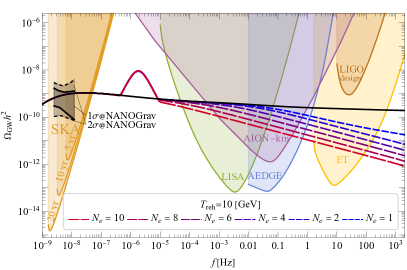
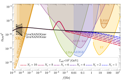
Figure 1: GW spectra from a supercooled phase transition and cosmic strings. The thick black line shows the cosmic string signal with no supercooled phase transition, while the coloured dashed lines show both sources for the number of efolds of supercooling indicated. The bump above the black line is the contribution from the transition itself, while the falling lines at higher frequencies illustrate how the string spectrum is impacted by the short inflation period associated with supercooling. For the strings, we used $G\mu=10^{-10}$ while for the PT $\beta/H=10$ in this example.

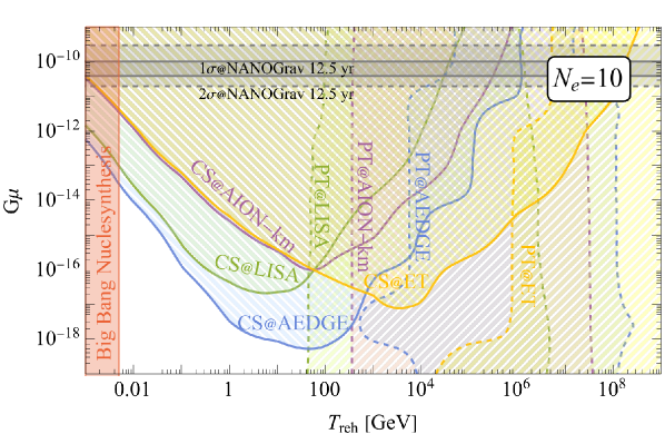
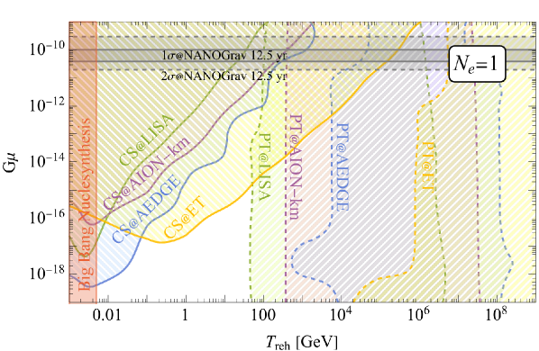
Figure 2: Part of the parameter space where our modified signals will be observed with $SNR>10$. We separate the calculation into the modified cosmic string tail (solid contours) and the phase transition contributions (dashed lines). We take into account only modified parts of the spectrum where the amplitude is at least $10\%$ away from the standard string spectrum with a given $G\mu$. For this example, we used $\beta/H=10$ for the PT, while the length of supercooling is taken to be $N_{e}=10$ (top panel) and $N_{e}=10$ (bottom panel).

VI Conclusion

Gravitational waves provide a pathway to test new high energy physics phenomena that took place in the early pre-BBN stages of the evolution of the universe. We considered a particularly well-motivated non-standard cosmological era known as supercooling or secondary inflation, and we studied its effects on the SGWB generated by a network of cosmic strings. Cosmic strings have a reasonably well understood GW emission spectrum. In particular, the emission during the standard radiation-dominated era results in a GW spectrum with a long flat plateau at high frequency. We can use this featureless spectrum to propagate through it various assumed cosmological histories and thus probe them with observational data.

In this paper, we have worked out in detail the structure imprinted on this SGWB by an epoch of supercooling. We find that such an early period of thermal inflation leaves a characteristic descending cosmic string plateau plus the peak produced at the end of supercooling. This can be used to distinguish thermal inflation from any other mechanism that can suppress the SGWB from strings at high frequencies, such as an early matter domination period (see Figure 1). The reason is that supercooling will forcibly end in a first order phase transition, whereas the other contributions might not.

For typical phase transition parameters with $\beta/H=10$ involving large supercooling, we found that detection prospects depend crucially on the length of the supercooling period if we aim to find spectra from both sources. For a very short thermal inflation period with $N_{e}=1$ the combined data from future experiments will probe the features of the spectrum with string tension above $G\mu=10^{-15}$ and only if the reheating temperature is around $T_{reh}=100$ GeV. For larger string tensions close to the ones fitting the NANOGrav signal the detection range extends to $T_{reh}\in[10^{2},10^{5}]$ GeV. For a long period of supercooling $N_{e}=10$ the detection prospects reach down to $G\mu=10^{-18}$ and extend to $T_{reh}\in[10^{2},10^{8}]$ GeV for strong string spectra close to PTA limits (see Figure 2). Crucially, these include both the emission from the strings and phase transition itself which can be used as a smoking gun to distinguish an epoch of supercooling from other modifications of the early universe evolution such as an era of early matter domination.

References

- (1) Particle Data Group collaboration, Review of Particle Physics, PTEP 2022 (2022) 083C01.
- (2) Planck collaboration, Planck 2018 results. VI. Cosmological parameters, Astron. Astrophys. 641 (2020) A6 [1807.06209].
- (3) R. Allahverdi et al., The First Three Seconds: a Review of Possible Expansion Histories of the Early Universe, 2006.16182.
- (4) P.J.E. Peebles and A. Vilenkin, Quintessential inflation, Phys. Rev. D 59 (1999) 063505 [astro-ph/9810509].
- (5) V. Poulin, T.L. Smith, D. Grin, T. Karwal and M. Kamionkowski, Cosmological implications of ultralight axionlike fields, Phys. Rev. D 98 (2018) 083525 [1806.10608].
- (6) LIGO Scientific, Virgo collaboration, Observation of Gravitational Waves from a Binary Black Hole Merger, Phys. Rev. Lett. 116 (2016) 061102 [1602.03837].
- (7) LIGO Scientific, Virgo collaboration, GWTC-1: A Gravitational-Wave Transient Catalog of Compact Binary Mergers Observed by LIGO and Virgo during the First and Second Observing Runs, Phys. Rev. X 9 (2019) 031040 [1811.12907].
- (8) LIGO Scientific, Virgo collaboration, GWTC-2: Compact Binary Coalescences Observed by LIGO and Virgo During the First Half of the Third Observing Run, Phys. Rev. X 11 (2021) 021053 [2010.14527].
- (9) LIGO Scientific, VIRGO collaboration, GWTC-2.1: Deep Extended Catalog of Compact Binary Coalescences Observed by LIGO and Virgo During the First Half of the Third Observing Run, 2108.01045.
- (10) LIGO Scientific, VIRGO, KAGRA collaboration, GWTC-3: Compact Binary Coalescences Observed by LIGO and Virgo During the Second Part of the Third Observing Run, 2111.03606.
- (11) M. Punturo et al., The Einstein Telescope: A third-generation gravitational wave observatory, Class. Quant. Grav. 27 (2010) 194002.
- (12) S. Hild et al., Sensitivity Studies for Third-Generation Gravitational Wave Observatories, Class. Quant. Grav. 28 (2011) 094013 [1012.0908].
- (13) G. Janssen et al., Gravitational wave astronomy with the SKA, PoS AASKA14 (2015) 037 [1501.00127].
- (14) P.W. Graham, J.M. Hogan, M.A. Kasevich and S. Rajendran, Resonant mode for gravitational wave detectors based on atom interferometry, Phys. Rev. D 94 (2016) 104022 [1606.01860].
- (15) LISA collaboration, Laser Interferometer Space Antenna, 1702.00786.
- (16) MAGIS collaboration, Mid-band gravitational wave detection with precision atomic sensors, 1711.02225.
- (17) L. Badurina et al., AION: An Atom Interferometer Observatory and Network, JCAP 05 (2020) 011 [1911.11755].
- (18) AEDGE collaboration, AEDGE: Atomic Experiment for Dark Matter and Gravity Exploration in Space, EPJ Quant. Technol. 7 (2020) 6 [1908.00802].
- (19) A. Bertoldi et al., AEDGE: Atomic experiment for dark matter and gravity exploration in space, Exper. Astron. 51 (2021) 1417.
- (20) I. Alonso et al., Cold atoms in space: community workshop summary and proposed road-map, EPJ Quant. Technol. 9 (2022) 30 [2201.07789].
- (21) L. Badurina, O. Buchmueller, J. Ellis, M. Lewicki, C. McCabe and V. Vaskonen, Prospective sensitivities of atom interferometers to gravitational waves and ultralight dark matter, Phil. Trans. A. Math. Phys. Eng. Sci. 380 (2021) 20210060 [2108.02468].
- (22) LISA Cosmology Working Group collaboration, Cosmology with the Laser Interferometer Space Antenna, 2204.05434.
- (23) M. Lewicki and V. Vaskonen, Impact of LIGO-Virgo black hole binaries on gravitational wave background searches, Eur. Phys. J. C 83 (2023) 168 [2111.05847].
- (24) NANOGrav collaboration, The NANOGrav 12.5 yr Data Set: Search for an Isotropic Stochastic Gravitational-wave Background, Astrophys. J. Lett. 905 (2020) L34 [2009.04496].
- (25) B. Goncharov et al., On the Evidence for a Common-spectrum Process in the Search for the Nanohertz Gravitational-wave Background with the Parkes Pulsar Timing Array, Astrophys. J. Lett. 917 (2021) L19 [2107.12112].
- (26) S. Chen et al., Common-red-signal analysis with 24-yr high-precision timing of the European Pulsar Timing Array: inferences in the stochastic gravitational-wave background search, Mon. Not. Roy. Astron. Soc. 508 (2021) 4970 [2110.13184].
- (27) J. Antoniadis et al., The International Pulsar Timing Array second data release: Search for an isotropic gravitational wave background, Mon. Not. Roy. Astron. Soc. 510 (2022) 4873 [2201.03980].
- (28) V. Vaskonen and H. Veermäe, Did NANOGrav see a signal from primordial black hole formation?, Phys. Rev. Lett. 126 (2021) 051303 [2009.07832].
- (29) V. De Luca, G. Franciolini and A. Riotto, NANOGrav Data Hints at Primordial Black Holes as Dark Matter, Phys. Rev. Lett. 126 (2021) 041303 [2009.08268].
- (30) Y. Nakai, M. Suzuki, F. Takahashi and M. Yamada, Gravitational Waves and Dark Radiation from Dark Phase Transition: Connecting NANOGrav Pulsar Timing Data and Hubble Tension, Phys. Lett. B 816 (2021) 136238 [2009.09754].
- (31) W. Ratzinger and P. Schwaller, Whispers from the dark side: Confronting light new physics with NANOGrav data, SciPost Phys. 10 (2021) 047 [2009.11875].
- (32) K. Kohri and T. Terada, Solar-Mass Primordial Black Holes Explain NANOGrav Hint of Gravitational Waves, Phys. Lett. B 813 (2021) 136040 [2009.11853].
- (33) S. Vagnozzi, Implications of the NANOGrav results for inflation, Mon. Not. Roy. Astron. Soc. 502 (2021) L11 [2009.13432].
- (34) A. Neronov, A. Roper Pol, C. Caprini and D. Semikoz, NANOGrav signal from magnetohydrodynamic turbulence at the QCD phase transition in the early Universe, Phys. Rev. D 103 (2021) 041302 [2009.14174].
- (35) J.J. Blanco-Pillado, K.D. Olum and J.M. Wachter, Comparison of cosmic string and superstring models to NANOGrav 12.5-year results, Phys. Rev. D 103 (2021) 103512 [2102.08194].
- (36) D. Wang, Squeezing Cosmological Phase Transitions with International Pulsar Timing Array, 2201.09295.
- (37) A. Roper Pol, C. Caprini, A. Neronov and D. Semikoz, Gravitational wave signal from primordial magnetic fields in the Pulsar Timing Array frequency band, Phys. Rev. D 105 (2022) 123502 [2201.05630].
- (38) R.Z. Ferreira, A. Notari, O. Pujolas and F. Rompineve, Gravitational waves from domain walls in Pulsar Timing Array datasets, JCAP 02 (2023) 001 [2204.04228].
- (39) J. Ellis and M. Lewicki, Cosmic String Interpretation of NANOGrav Pulsar Timing Data, Phys. Rev. Lett. 126 (2021) 041304 [2009.06555].
- (40) S. Blasi, V. Brdar and K. Schmitz, Has NANOGrav found first evidence for cosmic strings?, Phys. Rev. Lett. 126 (2021) 041305 [2009.06607].
- (41) NANOGrav Collaboration collaboration, The NANOGrav 15-year Data Set: Evidence for a Gravitational-Wave Background, 2306.16213.
- (42) NANOGrav Collaboration collaboration, The NANOGrav 15-year Data Set: Observations and Timing of 68 Millisecond Pulsars, 2306.16217.
- (43) European Pulsar Timing Array Collaboration collaboration, The second data release from the European Pulsar Timing Array III. Search for gravitational wave signals, 2306.16214.
- (44) European Pulsar Timing Array Collaboration collaboration, The second data release from the European Pulsar Timing Array I. The dataset and timing analysis, 2306.16224.
- (45) Parkes Pulsar Timing Array Collaboration collaboration, The Parkes Pulsar Timing Array Third Data Release, 2306.16230.
- (46) Parkes Pulsar Timing Array Collaboration collaboration, Search for an isotropic gravitational-wave background with the Parkes Pulsar Timing Array, 2306.16215.
- (47) Chinese Pulsar Timing Array Collaboration collaboration, Searching for the nano-Hertz stochastic gravitational wave background with the Chinese Pulsar Timing Array Data Release I, 2306.16216.
- (48) J. Ellis, M. Lewicki, C. Lin and V. Vaskonen, Cosmic Superstrings Revisited in Light of NANOGrav 15-Year Data, 2306.17147.
- (49) NANOGrav Collaboration collaboration, The NANOGrav 15-year Data Set: Constraints on Supermassive Black Hole Binaries from the Gravitational Wave Background, 2306.16220.
- (50) J. Antoniadis et al., The second data release from the European Pulsar Timing Array: V. Implications for massive black holes, dark matter and the early Universe, 2306.16227.
- (51) A. Vilenkin, Gravitational radiation from cosmic strings, Phys. Lett. B 107 (1981) 47.
- (52) C.J. Hogan and M.J. Rees, Gravitational interactions of cosmic strings, Nature 311 (1984) 109.
- (53) T. Vachaspati and A. Vilenkin, Gravitational Radiation from Cosmic Strings, Phys. Rev. D 31 (1985) 3052.
- (54) F.S. Accetta and L.M. Krauss, The stochastic gravitational wave spectrum resulting from cosmic string evolution, Nucl. Phys. B 319 (1989) 747.
- (55) D.P. Bennett and F.R. Bouchet, Constraints on the gravity wave background generated by cosmic strings, Phys. Rev. D 43 (1991) 2733.
- (56) R.R. Caldwell and B. Allen, Cosmological constraints on cosmic string gravitational radiation, Phys. Rev. D 45 (1992) 3447.
- (57) B. Allen and E.P.S. Shellard, Gravitational radiation from cosmic strings, Phys. Rev. D 45 (1992) 1898.
- (58) R.A. Battye, R.R. Caldwell and E.P.S. Shellard, Gravitational waves from cosmic strings, in Conference on Topological Defects and CMB, pp. 11–31, 6, 1997 [astro-ph/9706013].
- (59) M.R. DePies and C.J. Hogan, Stochastic Gravitational Wave Background from Light Cosmic Strings, Phys. Rev. D 75 (2007) 125006 [astro-ph/0702335].
- (60) X. Siemens, V. Mandic and J. Creighton, Gravitational wave stochastic background from cosmic (super)strings, Phys. Rev. Lett. 98 (2007) 111101 [astro-ph/0610920].
- (61) S. Olmez, V. Mandic and X. Siemens, Gravitational-Wave Stochastic Background from Kinks and Cusps on Cosmic Strings, Phys. Rev. D 81 (2010) 104028 [1004.0890].
- (62) T. Regimbau, S. Giampanis, X. Siemens and V. Mandic, The stochastic background from cosmic (super)strings: popcorn and (Gaussian) continuous regimes, Phys. Rev. D 85 (2012) 066001 [1111.6638].
- (63) S.A. Sanidas, R.A. Battye and B.W. Stappers, Constraints on cosmic string tension imposed by the limit on the stochastic gravitational wave background from the European Pulsar Timing Array, Phys. Rev. D 85 (2012) 122003 [1201.2419].
- (64) S.A. Sanidas, R.A. Battye and B.W. Stappers, Projected constraints on the cosmic (super)string tension with future gravitational wave detection experiments, Astrophys. J. 764 (2013) 108 [1211.5042].
- (65) P. Binetruy, A. Bohe, C. Caprini and J.-F. Dufaux, Cosmological Backgrounds of Gravitational Waves and eLISA/NGO: Phase Transitions, Cosmic Strings and Other Sources, JCAP 06 (2012) 027 [1201.0983].
- (66) S. Kuroyanagi, K. Miyamoto, T. Sekiguchi, K. Takahashi and J. Silk, Forecast constraints on cosmic string parameters from gravitational wave direct detection experiments, Phys. Rev. D 86 (2012) 023503 [1202.3032].
- (67) S. Kuroyanagi, K. Miyamoto, T. Sekiguchi, K. Takahashi and J. Silk, Forecast constraints on cosmic strings from future CMB, pulsar timing and gravitational wave direct detection experiments, Phys. Rev. D 87 (2013) 023522 [1210.2829].
- (68) L. Sousa and P.P. Avelino, Probing Cosmic Superstrings with Gravitational Waves, Phys. Rev. D 94 (2016) 063529 [1606.05585].
- (69) L. Sousa, P.P. Avelino and G.S.F. Guedes, Full analytical approximation to the stochastic gravitational wave background generated by cosmic string networks, Phys. Rev. D 101 (2020) 103508 [2002.01079].
- (70) Y. Cui, M. Lewicki, D.E. Morrissey and J.D. Wells, Cosmic Archaeology with Gravitational Waves from Cosmic Strings, Phys. Rev. D 97 (2018) 123505 [1711.03104].
- (71) Y. Cui, M. Lewicki, D.E. Morrissey and J.D. Wells, Probing the pre-BBN universe with gravitational waves from cosmic strings, JHEP 01 (2019) 081 [1808.08968].
- (72) P. Auclair et al., Probing the gravitational wave background from cosmic strings with LISA, JCAP 04 (2020) 034 [1909.00819].
- (73) G.S.F. Guedes, P.P. Avelino and L. Sousa, Signature of inflation in the stochastic gravitational wave background generated by cosmic string networks, Phys. Rev. D 98 (2018) 123505 [1809.10802].
- (74) N. Ramberg and L. Visinelli, Probing the Early Universe with Axion Physics and Gravitational Waves, Phys. Rev. D 99 (2019) 123513 [1904.05707].
- (75) Y. Gouttenoire, G. Servant and P. Simakachorn, Beyond the Standard Models with Cosmic Strings, JCAP 07 (2020) 032 [1912.02569].
- (76) Y. Gouttenoire, G. Servant and P. Simakachorn, BSM with Cosmic Strings: Heavy, up to EeV mass, Unstable Particles, JCAP 07 (2020) 016 [1912.03245].
- (77) C.-F. Chang and Y. Cui, Stochastic Gravitational Wave Background from Global Cosmic Strings, Phys. Dark Univ. 29 (2020) 100604 [1910.04781].
- (78) Y. Cui, M. Lewicki and D.E. Morrissey, Gravitational Wave Bursts as Harbingers of Cosmic Strings Diluted by Inflation, Phys. Rev. Lett. 125 (2020) 211302 [1912.08832].
- (79) Y. Gouttenoire, G. Servant and P. Simakachorn, Kination cosmology from scalar fields and gravitational-wave signatures, 2111.01150.
- (80) P. Creminelli, A. Nicolis and R. Rattazzi, Holography and the electroweak phase transition, JHEP 03 (2002) 051 [hep-th/0107141].
- (81) L. Randall and G. Servant, Gravitational waves from warped spacetime, JHEP 05 (2007) 054 [hep-ph/0607158].
- (82) G. Nardini, M. Quiros and A. Wulzer, A Confining Strong First-Order Electroweak Phase Transition, JHEP 09 (2007) 077 [0706.3388].
- (83) T. Konstandin and G. Servant, Cosmological Consequences of Nearly Conformal Dynamics at the TeV scale, JCAP 12 (2011) 009 [1104.4791].
- (84) B. von Harling and G. Servant, QCD-induced Electroweak Phase Transition, JHEP 01 (2018) 159 [1711.11554].
- (85) S. Iso, P.D. Serpico and K. Shimada, QCD-Electroweak First-Order Phase Transition in a Supercooled Universe, Phys. Rev. Lett. 119 (2017) 141301 [1704.04955].
- (86) S. Bruggisser, B. Von Harling, O. Matsedonskyi and G. Servant, Electroweak Phase Transition and Baryogenesis in Composite Higgs Models, JHEP 12 (2018) 099 [1804.07314].
- (87) P. Baratella, A. Pomarol and F. Rompineve, The Supercooled Universe, JHEP 03 (2019) 100 [1812.06996].
- (88) K. Agashe, P. Du, M. Ekhterachian, S. Kumar and R. Sundrum, Cosmological Phase Transition of Spontaneous Confinement, JHEP 05 (2020) 086 [1910.06238].
- (89) L. Delle Rose, G. Panico, M. Redi and A. Tesi, Gravitational Waves from Supercool Axions, JHEP 04 (2020) 025 [1912.06139].
- (90) B. Von Harling, A. Pomarol, O. Pujolàs and F. Rompineve, Peccei-Quinn Phase Transition at LIGO, JHEP 04 (2020) 195 [1912.07587].
- (91) C. Caprini et al., Detecting gravitational waves from cosmological phase transitions with LISA: an update, JCAP 03 (2020) 024 [1910.13125].
- (92) I. Baldes, Y. Gouttenoire and F. Sala, String Fragmentation in Supercooled Confinement and Implications for Dark Matter, JHEP 04 (2021) 278 [2007.08440].
- (93) L. Sagunski, P. Schicho and D. Schmitt, Supercool exit: Gravitational waves from QCD-triggered conformal symmetry breaking, 2303.02450.
- (94) R. Jinno and M. Takimoto, Probing a classically conformal B-L model with gravitational waves, Phys. Rev. D 95 (2017) 015020 [1604.05035].
- (95) L. Marzola, A. Racioppi and V. Vaskonen, Phase transition and gravitational wave phenomenology of scalar conformal extensions of the Standard Model, Eur. Phys. J. C 77 (2017) 484 [1704.01034].
- (96) T. Prokopec, J. Rezacek and B. Świeżewska, Gravitational waves from conformal symmetry breaking, JCAP 02 (2019) 009 [1809.11129].
- (97) C. Marzo, L. Marzola and V. Vaskonen, Phase transition and vacuum stability in the classically conformal B–L model, Eur. Phys. J. C 79 (2019) 601 [1811.11169].
- (98) B. Von Harling, A. Pomarol, O. Pujolàs and F. Rompineve, Peccei-Quinn Phase Transition at LIGO, JHEP 04 (2020) 195 [1912.07587].
- (99) M. Aoki and J. Kubo, Gravitational waves from chiral phase transition in a conformally extended standard model, JCAP 04 (2020) 001 [1910.05025].
- (100) X. Wang, F.P. Huang and X. Zhang, Phase transition dynamics and gravitational wave spectra of strong first-order phase transition in supercooled universe, JCAP 05 (2020) 045 [2003.08892].
- (101) J. Ellis, M. Lewicki and V. Vaskonen, Updated predictions for gravitational waves produced in a strongly supercooled phase transition, JCAP 11 (2020) 020 [2007.15586].
- (102) A. Ghoshal and A. Salvio, Gravitational waves from fundamental axion dynamics, JHEP 12 (2020) 049 [2007.00005].
- (103) M. Lewicki, O. Pujolàs and V. Vaskonen, Escape from supercooling with or without bubbles: gravitational wave signatures, Eur. Phys. J. C 81 (2021) 857 [2106.09706].
- (104) A. Dasgupta, P.S.B. Dev, A. Ghoshal and A. Mazumdar, Gravitational wave pathway to testable leptogenesis, Phys. Rev. D 106 (2022) 075027 [2206.07032].
- (105) M. Kierkla, A. Karam and B. Swiezewska, Conformal model for gravitational waves and dark matter: a status update, JHEP 03 (2023) 007 [2210.07075].
- (106) X. Wong and K.-P. Xie, Freeze-in of WIMP dark matter, 2304.00908.
- (107) A. Salvio, Model-Independent Radiative Symmetry Breaking and Gravitational Waves, 2302.10212.
- (108) J. Ellis, M. Lewicki and J.M. No, On the Maximal Strength of a First-Order Electroweak Phase Transition and its Gravitational Wave Signal, JCAP 04 (2019) 003 [1809.08242].
- (109) J. Ellis, M. Lewicki, J.M. No and V. Vaskonen, Gravitational wave energy budget in strongly supercooled phase transitions, JCAP 06 (2019) 024 [1903.09642].
- (110) J. Ellis, M. Lewicki and J.M. No, Gravitational waves from first-order cosmological phase transitions: lifetime of the sound wave source, JCAP 07 (2020) 050 [2003.07360].
- (111) T.W.B. Kibble, Topology of Cosmic Domains and Strings, J. Phys. A 9 (1976) 1387.
- (112) T.W.B. Kibble, Some Implications of a Cosmological Phase Transition, Phys. Rept. 67 (1980) 183.
- (113) M.B. Hindmarsh and T.W.B. Kibble, Cosmic strings, Rept. Prog. Phys. 58 (1995) 477 [hep-ph/9411342].
- (114) A. Vilenkin and E.P.S. Shellard, Cosmic Strings and Other Topological Defects, Cambridge University Press (7, 2000).
- (115) V. Vanchurin, K.D. Olum and A. Vilenkin, Scaling of cosmic string loops, Phys. Rev. D 74 (2006) 063527 [gr-qc/0511159].
- (116) C.J.A.P. Martins and E.P.S. Shellard, Fractal properties and small-scale structure of cosmic string networks, Phys. Rev. D 73 (2006) 043515 [astro-ph/0511792].
- (117) J.J. Blanco-Pillado, K.D. Olum and B. Shlaer, Large parallel cosmic string simulations: New results on loop production, Phys. Rev. D 83 (2011) 083514 [1101.5173].
- (118) R.J. Scherrer and J.A. Frieman, Cosmic strings as random walks, Phys. Rev. D 33 (1986) 3556.
- (119) C.J.A.P. Martins and E.P.S. Shellard, String evolution with friction, Phys. Rev. D 53 (1996) 575 [hep-ph/9507335].
- (120) C.J.A.P. Martins and E.P.S. Shellard, Quantitative string evolution, Phys. Rev. D 54 (1996) 2535 [hep-ph/9602271].
- (121) C.J.A.P. Martins and E.P.S. Shellard, Extending the velocity dependent one scale string evolution model, Phys. Rev. D 65 (2002) 043514 [hep-ph/0003298].
- (122) P.P. Avelino and L. Sousa, Scaling laws for weakly interacting cosmic (super)string and p-brane networks, Phys. Rev. D 85 (2012) 083525 [1202.6298].
- (123) L. Sousa and P.P. Avelino, Stochastic Gravitational Wave Background generated by Cosmic String Networks: Velocity-Dependent One-Scale model versus Scale-Invariant Evolution, Phys. Rev. D 88 (2013) 023516 [1304.2445].
- (124) J.J. Blanco-Pillado, K.D. Olum and B. Shlaer, The number of cosmic string loops, Phys. Rev. D 89 (2014) 023512 [1309.6637].
- (125) J.J. Blanco-Pillado, K.D. Olum and B. Shlaer, Cosmic string loop shapes, Phys. Rev. D 92 (2015) 063528 [1508.02693].
- (126) J.J. Blanco-Pillado and K.D. Olum, Stochastic gravitational wave background from smoothed cosmic string loops, Phys. Rev. D 96 (2017) 104046 [1709.02693].
- (127) J.J. Blanco-Pillado, K.D. Olum and J.M. Wachter, Energy-conservation constraints on cosmic string loop production and distribution functions, Phys. Rev. D 100 (2019) 123526 [1907.09373].
- (128) J.J. Blanco-Pillado and K.D. Olum, Direct determination of cosmic string loop density from simulations, Phys. Rev. D 101 (2020) 103018 [1912.10017].
- (129) J.J. Blanco-Pillado, K.D. Olum and X. Siemens, New limits on cosmic strings from gravitational wave observation, Phys. Lett. B 778 (2018) 392 [1709.02434].
- (130) C. Caprini et al., Science with the space-based interferometer eLISA. II: Gravitational waves from cosmological phase transitions, JCAP 04 (2016) 001 [1512.06239].
- (131) A. Kosowsky and M.S. Turner, Gravitational radiation from colliding vacuum bubbles: envelope approximation to many bubble collisions, Phys. Rev. D 47 (1993) 4372 [astro-ph/9211004].
- (132) S.J. Huber and T. Konstandin, Gravitational Wave Production by Collisions: More Bubbles, JCAP 09 (2008) 022 [0806.1828].
- (133) M. Lewicki and V. Vaskonen, On bubble collisions in strongly supercooled phase transitions, Phys. Dark Univ. 30 (2020) 100672 [1912.00997].
- (134) M. Lewicki and V. Vaskonen, Gravitational waves from colliding vacuum bubbles in gauge theories, Eur. Phys. J. C 81 (2021) 437 [2012.07826].
- (135) M. Lewicki and V. Vaskonen, Gravitational wave spectra from strongly supercooled phase transitions, Eur. Phys. J. C 80 (2020) 1003 [2007.04967].
- (136) M. Kamionkowski, A. Kosowsky and M.S. Turner, Gravitational radiation from first order phase transitions, Phys. Rev. D 49 (1994) 2837 [astro-ph/9310044].
- (137) M. Hindmarsh, S.J. Huber, K. Rummukainen and D.J. Weir, Gravitational waves from the sound of a first order phase transition, Phys. Rev. Lett. 112 (2014) 041301 [1304.2433].
- (138) M. Hindmarsh, S.J. Huber, K. Rummukainen and D.J. Weir, Numerical simulations of acoustically generated gravitational waves at a first order phase transition, Phys. Rev. D 92 (2015) 123009 [1504.03291].
- (139) M. Hindmarsh, S.J. Huber, K. Rummukainen and D.J. Weir, Shape of the acoustic gravitational wave power spectrum from a first order phase transition, Phys. Rev. D 96 (2017) 103520 [1704.05871].
- (140) M.B. Hindmarsh, M. Lüben, J. Lumma and M. Pauly, Phase transitions in the early universe, SciPost Phys. Lect. Notes 24 (2021) 1 [2008.09136].
- (141) A. Roper Pol, S. Mandal, A. Brandenburg, T. Kahniashvili and A. Kosowsky, Numerical simulations of gravitational waves from early-universe turbulence, Phys. Rev. D 102 (2020) 083512 [1903.08585].
- (142) T. Kahniashvili, A. Brandenburg, G. Gogoberidze, S. Mandal and A. Roper Pol, Circular polarization of gravitational waves from early-Universe helical turbulence, Phys. Rev. Res. 3 (2021) 013193 [2011.05556].
- (143) A. Roper Pol, S. Mandal, A. Brandenburg and T. Kahniashvili, Polarization of gravitational waves from helical MHD turbulent sources, JCAP 04 (2022) 019 [2107.05356].
- (144) P. Auclair, C. Caprini, D. Cutting, M. Hindmarsh, K. Rummukainen, D.A. Steer et al., Generation of gravitational waves from freely decaying turbulence, JCAP 09 (2022) 029 [2205.02588].
- (145) B. Laurent and J.M. Cline, Fluid equations for fast-moving electroweak bubble walls, Phys. Rev. D 102 (2020) 063516 [2007.10935].
- (146) J.M. Cline, A. Friedlander, D.-M. He, K. Kainulainen, B. Laurent and D. Tucker-Smith, Baryogenesis and gravity waves from a UV-completed electroweak phase transition, Phys. Rev. D 103 (2021) 123529 [2102.12490].
- (147) M. Lewicki, M. Merchand and M. Zych, Electroweak bubble wall expansion: gravitational waves and baryogenesis in Standard Model-like thermal plasma, JHEP 02 (2022) 017 [2111.02393].
- (148) B. Laurent and J.M. Cline, First principles determination of bubble wall velocity, Phys. Rev. D 106 (2022) 023501 [2204.13120].
- (149) J. Ellis, M. Lewicki, M. Merchand, J.M. No and M. Zych, The scalar singlet extension of the Standard Model: gravitational waves versus baryogenesis, JHEP 01 (2023) 093 [2210.16305].
- (150) J.R. Espinosa, T. Konstandin, J.M. No and G. Servant, Energy Budget of Cosmological First-order Phase Transitions, JCAP 06 (2010) 028 [1004.4187].
- (151) R. Jinno, H. Seong, M. Takimoto and C.M. Um, Gravitational waves from first-order phase transitions: Ultra-supercooled transitions and the fate of relativistic shocks, JCAP 10 (2019) 033 [1905.00899].
- (152) M. Lewicki and V. Vaskonen, Gravitational waves from bubble collisions and fluid motion in strongly supercooled phase transitions, Eur. Phys. J. C 83 (2023) 109 [2208.11697].
- (153) K. Saikawa and S. Shirai, Primordial gravitational waves, precisely: The role of thermodynamics in the Standard Model, JCAP 05 (2018) 035 [1803.01038].
- (154) N. Bartolo et al., Science with the space-based interferometer LISA. IV: Probing inflation with gravitational waves, JCAP 12 (2016) 026 [1610.06481].
- (155) C. Caprini, D.G. Figueroa, R. Flauger, G. Nardini, M. Peloso, M. Pieroni et al., Reconstructing the spectral shape of a stochastic gravitational wave background with LISA, JCAP 11 (2019) 017 [1906.09244].
- (156) AEDGE collaboration, AEDGE: Atomic Experiment for Dark Matter and Gravity Exploration in Space, EPJ Quant. Technol. 7 (2020) 6 [1908.00802].
- (157) LIGO Scientific collaboration, Advanced LIGO, Class. Quant. Grav. 32 (2015) 074001 [1411.4547].
- (158) E. Thrane and J.D. Romano, Sensitivity curves for searches for gravitational-wave backgrounds, Phys. Rev. D 88 (2013) 124032 [1310.5300].
- (159) LIGO Scientific, Virgo collaboration, GW150914: Implications for the stochastic gravitational wave background from binary black holes, Phys. Rev. Lett. 116 (2016) 131102 [1602.03847].
- (160) LIGO Scientific, Virgo collaboration, Search for the isotropic stochastic background using data from Advanced LIGO’s second observing run, Phys. Rev. D 100 (2019) 061101 [1903.02886].