Mapping historical forest biomass for stock-change assessments at parcel to landscape scales

Abstract

Understanding historical forest dynamics, specifically changes in forest biomass and carbon stocks, has become critical for assessing current forest climate benefits and projecting future benefits under various policy, regulatory, and stewardship scenarios. Carbon accounting frameworks based exclusively on national forest inventories are limited to broad-scale estimates, but model-based approaches that combine these inventories with remotely sensed data can yield contiguous fine-resolution maps of forest biomass and carbon stocks across landscapes over time. Here we describe a fundamental step in building a map-based stock-change framework: mapping historical forest biomass at fine temporal and spatial resolution (annual, 30m) across all of New York State (USA) from 1990 to 2019, using freely available data and open-source tools.

Using Landsat imagery, US Forest Service Forest Inventory and Analysis (FIA) data, and off-the-shelf LiDAR collections we developed three modeling approaches for mapping historical forest aboveground biomass (AGB): training on FIA plot-level AGB estimates (direct), training on LiDAR-derived AGB maps (indirect), and an ensemble averaging predictions from the direct and indirect models. Model prediction surfaces (maps) were tested against FIA estimates at multiple scales. All three approaches produced viable outputs, yet tradeoffs were evident in terms of model complexity, map accuracy, saturation, and fine-scale pattern representation. The resulting map products can help identify where, when, and how forest carbon stocks are changing as a result of both anthropogenic and natural drivers alike. These products can thus serve as inputs to a wide range of applications including stock-change assessments, monitoring reporting and verification frameworks, and prioritizing parcels for protection or enrollment in improved management programs.

Keywords Landsat • LiDAR • aboveground biomass • machine learning • land cover

1 Introduction

Forests are among the most effective natural carbon sinks and thus are essential in stabilizing Earth’s climate, but their capacity to provide this critical service has been strongly shaped by past and present anthropogenic impacts. Understanding the spatiotemporal dynamics of forest carbon in relation to human activities has become increasingly important as policymakers and stakeholders look to nature-based solutions to reduce atmospheric greenhouse gas (GHG) concentrations and mitigate climate change (Malmsheimer et al. 2008; Fargione et al. 2018). With a better grasp of local social and ecological conditions across the forest landscape, decision-makers could identify and prioritize parcels of land suitable for different strategies such as reforestation, avoided conversion, or enhanced forest management, in order to sustain and/or increase carbon sequestration and effectively offset GHG emissions from other sectors (Houghton 2005; Houghton et al. 2012). To quantify potential climate benefits, carbon status and trends are typically assessed using a stock-change methodology that requires historical data and ongoing monitoring efforts via permanent plot networks.

National forest inventories (NFI) like the USDA’s Forest Inventory and Analysis (FIA) program provide estimates of forest biomass, carbon stocks, and stock-changes at large scales based on their extensive sampling design. Although these programs have offered fundamental insights and essential data on forest carbon dynamics over the past three decades (Buendia et al. 2019; Woodall et al. 2015), they are limited spatially by the sample density and remeasurement frequency (McRoberts 2011), and thus cannot represent fine-scaled patterns and dynamics most relevant to planning and decision-making. Model-based approaches, which combine field data like the FIA with wall-to-wall remotely-sensed data can fill this need by producing predictions for all map units (pixels) in a given area.

Largely due to limitations of the available data, implementing model-based approaches for characterizing historical spatiotemporal dynamics of forest carbon remains challenging. Remotely-sensed data best describes the most prominent aboveground components of a forest, and for this reason aboveground biomass (AGB) often serves as an initial target variable (Houghton, Hall, and Goetz 2009) before empirical conversions to specific carbon pools are made (Heath et al. 2009; Woodall et al. 2011). Airborne LiDAR has been established as a highly valuable remotely-sensed data source for such AGB mapping efforts, but is often collected for irregularly defined boundaries at local to regional scales, resulting in spatiotemporal patchworks when pooled together for broad-scale applications (Johnson et al. 2022; Huang et al. 2019; Skowronski and Lister 2012). Remotely-sensed optical imagery offers far better spatial coverage and temporal consistency than airborne LiDAR point clouds, but cannot characterize forest structure with the same level of detail nor at the same spatial resolution. Optical datasets still provide the best set of historical earth surface observations available; in particular, the Landsat program offering spectral information at a 30 m resolution for the past four decades has supported a broad array of historical time series mapping efforts (Hansen and Loveland 2012; Banskota et al. 2014; Wulder et al. 2022). More recent spaceborne remote sensing missions that collect LiDAR and synthetic aperture radar (SAR) may offer benefits for quantifying forest structure at similarly broad scales, but these platforms cannot match the historical continuity offered by Landsat (Dubayah et al. 2014; Abdalati et al. 2010; Torres et al. 2012; Rosenqvist et al. 2007).

A handful of studies have used Landsat time series imagery for multi-annual, fine-resolution, broad-scale AGB mapping (Kennedy, Ohmann, et al. 2018; Matasci et al. 2018; Hudak et al. 2020). These efforts can be categorized into ‘direct’ approaches, where models were fit using AGB measurements from FIA field plots (Kennedy, Ohmann, et al. 2018), and ‘indirect’ approaches, where models were fit to AGB predictions from separate models trained with LiDAR data (Matasci et al. 2018; Hudak et al. 2020). Direct approaches offer a degree of parsimony relative to their indirect counterparts, and limit the propagation of errors through multiple stages of modeling. Indirect approaches could yield more accurate predictions due to the availability of a larger model training sample comprised of LiDAR-based predictions (pixels). In theory a sample of LiDAR-based predictions would cover a wider range of AGB conditions, have improved geolocation accuracy, and offer better spatial compatibility with Landsat pixels relative to traditional field plots (Hudak et al. 2020). These two overarching approaches (direct and indirect) have only been compared for snapshots in time (single year mapping), over a relatively small (820,000 ha) and homogenous section of boreal forest in Alaska (Strunk et al. 2014), as well as over Mexico with the Mexican NFI and the addition of SAR data (Urbazaev et al. 2018).

In this paper, as part of a broader effort for map-based forest carbon accounting across New York State (NYS), we present methods for translating FIA’s discrete plot-based inventory to 30 years (1990-2019) of annual statewide AGB maps at a 30 m resolution. The resulting map products provide the necessary data to replicate FIA’s stock-change accounting approach in a spatially explicit manner with the flexibility to produce outputs at scales ranging from individual parcels to the entire state. The models we developed to achieve these ends demonstrate what is to our knowledge the first attempt to synthesize direct and indirect approaches. We used Landsat time series imagery, FIA plots, and publicly available off-the-shelf LiDAR data to develop an ensemble of these two distinct modeling strategies (direct and indirect) that leveraged their relative strengths and improved the predictive accuracy of our overall approach. We assessed agreement between mapped predictions from all three approaches (direct, indirect, and ensemble) and an independent set of FIA estimates across a range of scales. These methods using publicly available data and open-source tools are flexible, efficient, and extensible in space and time, thus providing a framework for those seeking to develop maps of forest AGB dynamics for both retrospective and monitoring objectives alike. Results produced following this framework not only provide inputs for stock-change analyses at scales germane to management, but will also broadly support forest stewardship, future research, and ongoing planning.

2 Data and methods

2.1 Overview

We developed three modeling approaches (Figure 1) to map aboveground biomass (AGB) annually across New York State (NYS). The direct approach used AGB estimates at USDA Forest Inventory and Analysis (FIA; Gray et al. (2012)) field plots as a dependent variable. The indirect approach used LiDAR-based predictions of AGB developed by Johnson et al. (2022) as a dependent variable. For both approaches, the respective dependent variables were associated with predictors derived from temporally matching Landsat imagery and landcover classifications, as well as temporally static climate, topographic, and ecological layers. We used each of these combined datasets to produce separate stacked ensemble models composed of several machine learning (ML) models. Predictions from these two approaches were averaged to create a third ensemble approach. Each of the three modeling approaches were used to make annual (1990-2019) AGB predictions at a 30m resolution across the entire state, and the resulting maps were assessed with a common set of independent FIA plots.

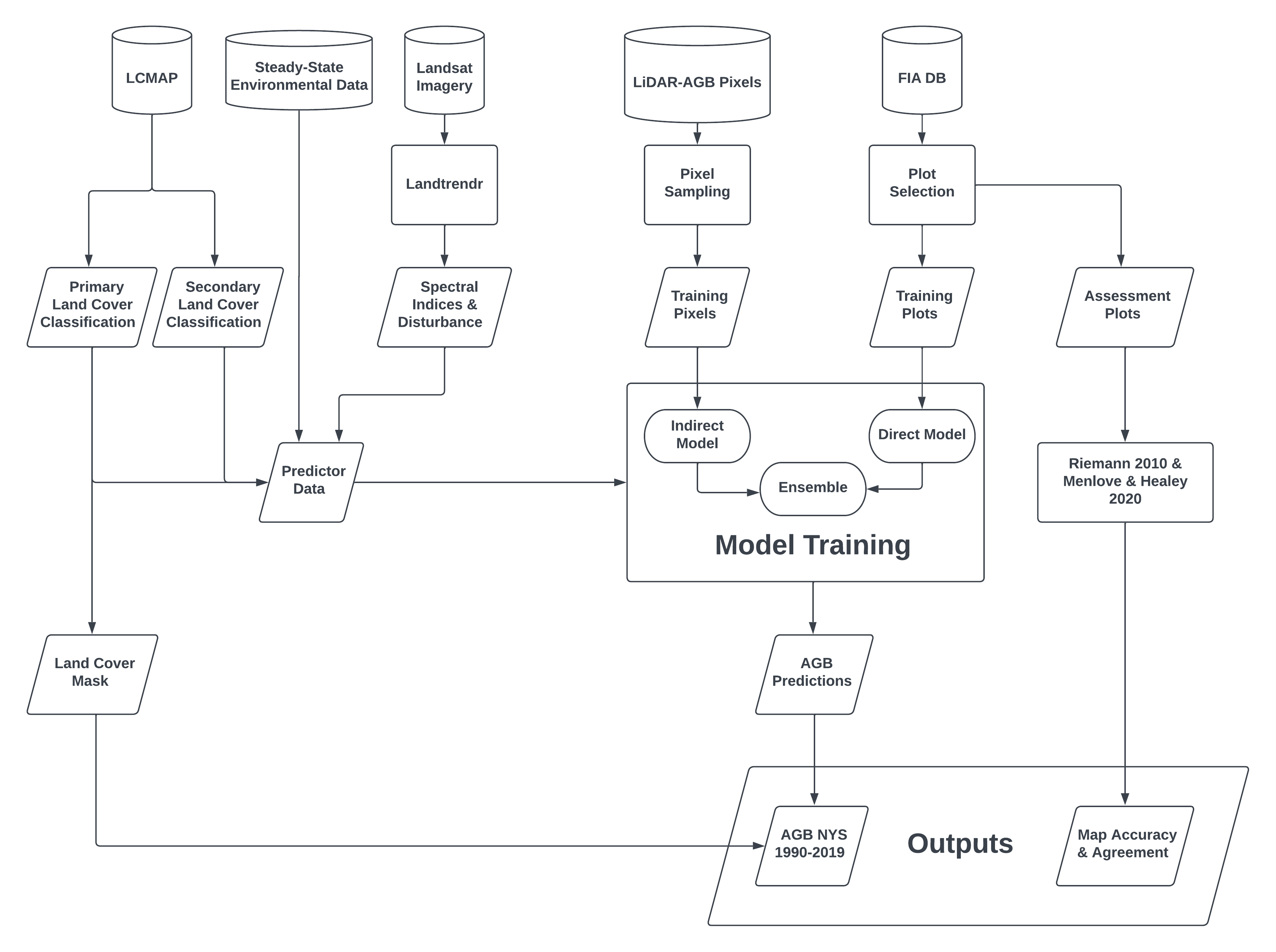
Figure 1: A flowchart diagram showing the key elements of the modeling and mapping methodology. Cylinders represent data repositories, parallelograms represent data products and results, rectangles represent processing steps, and ovals represent models.

2.2 Study area

NYS covers 141,297 km² in the Northeastern US and was approximately 59% forested as of 2019 (USFS 2020). The forests are dominated by Northern hardwoods-hemlock types but include Appalachian oak and beech-maple-basswood forests in the western and southern regions of the state respectively (Dyer 2006). Like much of the US Northeast, NYS was extensively deforested during the 18th and 19th centuries, with subsequent reforestation, and conservation resulting in a landscape dominated by forest stands that are now over 100 years old (Whitney 1994; Lorimer 2001; Michael J. Mahoney et al. 2022). NYS created the Forest Preserve in 1885, establishing the foundation for what became the Adirondack and Catskill Parks decades later. Any state-owned or acquired lands within these parks has since been designated as ‘forever wild’ and has largely been protected from timber harvesting. More recent land use dynamics indicate that total agricultural area has continued to decline in the state and has been replaced by similar extents of forested and developed lands (Widmann et al. 2012; Widmann 2016). Total forest area was estimated to have peaked as of 2012 and forest loss due to continued human development has recently outpaced gains due to agricultural abandonment (Widmann 2016; USFS 2020). Harvesting activities, weather-related events, and insect outbreaks drive disturbance and damage patterns within consistently forested areas (Kosiba et al. 2018; USFS 2020).

2.3 Field data

Two field datasets were compiled from the FIA inventory in NYS for the distinct purposes of model development and map assessment. The FIA program compiled AGB estimates for trees $\geq$ 12.7 cm (5 in) diameter at breast height (Gray et al. 2012), and were converted to units of megagrams per hectare (Mg ha^-1). The FIA uses permanent inventory plots arranged in a quasi-systematic hexagonal grid that are divided into five panels, each assumed to have complete spatial coverage over the state, and remeasured on a 5–7 year basis (Bechtold and Patterson 2005). Tree measurements, and subsequently AGB estimates based on allometrics, were only recorded on portions of plots considered forested. For an area to be considered forested by the FIA, the area must be at least 10% stocked with trees, at least 0.4 ha (1 acre) in size, and at least 36.58 m (120 ft) wide. Any lands meeting these minimum requirements, but developed for nonforest land uses, were not considered forested. By this definition, it is likely that some nonforest conditions contained AGB that was not measured. In absence of additional information, however, we assumed that any nonforest conditions represented 0 AGB.

FIA plots are composed of four identical circular subplots with radii of 7.32 m (24 ft), with one subplot centered at the macroplot centroid and three subplots located 36.6 m (120 ft) away at azimuths of 360°, 120°, and 240° (Bechtold and Patterson 2005). The plot locations were provided by the FIA program in the form of average coordinates, collected over multiple repeat visits, representing the centroid of the center subplot, which we then used to build a polygon dataset representing the entire plot layout including all four subplots. Averaged coordinates were necessary due to the lack of precision of initial GPS coordinates for the macroplot centroids (Hoppus and Lister 2005; Cooke 2000). We use the phrase ‘FIA plot’ to refer to the aggregation of all four subplots.

We only considered FIA plots following the national plot design where all subplots were marked as measured. Importantly, excluding non-measured plots does not invalidate FIA’s probability sample because the FIA program assumes these plots to be randomly distributed across the landscape (Bechtold and Patterson 2005). Further, when available plots were inventoried more than once, single instances were selected randomly to avoid replication. These initial selection criteria resulted in a pool of 5,144 plots inventoried between 2002 and 2019. We then divided this set of plots into the model development and map assessment datasets using FIA’s panel designation, with one of the five panels randomly selected and all plots with this designation assigned to the map assessment dataset, and the remaining plots assigned to the model development dataset. In this way we partitioned 20% of the available plot data for an independent map assessment, yielding a probability sample with complete spatial coverage which we used to generate unbiased estimates of map agreement metrics (Stehman and Foody 2019; Riemann et al. 2010).

For the model development dataset we further selected the 1,954 completely forested plots to ensure that non-response in nonforest conditions would not degrade the relationship between predictors and plot-level AGB. However, to train and test our models with information covering the broadest possible range of conditions we added a set of 95 completely nonforested plots that were identified as true zeroes (AGB) based on LIDAR-derived maximum heights $\leq$ 1 m (Johnson et al. 2022). The model development dataset contained 2,049 unique plots (Table 1). For the map assessment dataset we filtered plots external to our mapped area based on our landcover mask (Section 2.7), as these plots were considered outside our population of interest, resulting in 545 total plots (Table 1).

Table 1: Annual counts of FIA plots divided into model development and map assessment datasets.

Year	Model Development	Map Assessment
2002	172
2003	188
2004	98
2005	106
2006	157
2007		207
2008	165
2009	146
2010	153
2011	174
2012		191
2013	138
2014	156
2015	119
2016	96
2017	129
2018	19	96
2019	33	51
Total	2049	545

2.4 LiDAR data and LiDAR pixel sampling

For our indirect modeling approach we used existing LiDAR-based AGB prediction surfaces as reference data for model training (Figure 2). Johnson et al. (2022) developed these 30 m surfaces with a spatio-temporal patchwork of 17 leaf-off LiDAR collections covering 62.46% (7,835,690 ha) of NYS. LiDAR data were collected from altitudes ranging from 700–5300 m with pulse densities ranging from 1.54–3.24 pulses per m². A set of 40 predictors computed from the height-normalized point clouds, in combination with topographic, climatic, landcover, and cadastral data were colocated with FIA plots as model training data. Stacked ensembles (Wolpert 1992) of machine learning models were used to make predictions across the patchwork; further details can be found in Johnson et al. (2022).

Following Johnson et al. (2022), we restricted the map space using a vegetation mask based on LCMAP primary classifications (Brown et al. 2020; Zhu and Woodcock 2014) as well as an area of applicability mask (Meyer and Pebesma 2021). As such, our sample of LiDAR-based AGB predictions was limited to vegetated landscapes, and where predictions were based on predictor data that was sufficiently represented in the training data. Following the indirect modeling efforts described in Hudak et al. (2020), we conducted a stratified random sample from the LiDAR-based AGB predictions, where strata were defined as 20 equal intervals ranging from 0 to the maximum mapped AGB value (~330 Mg ha^-1). 1,000 pixels were sampled from each stratum resulting in a total of 20,000 spatially resolved AGB predictions.

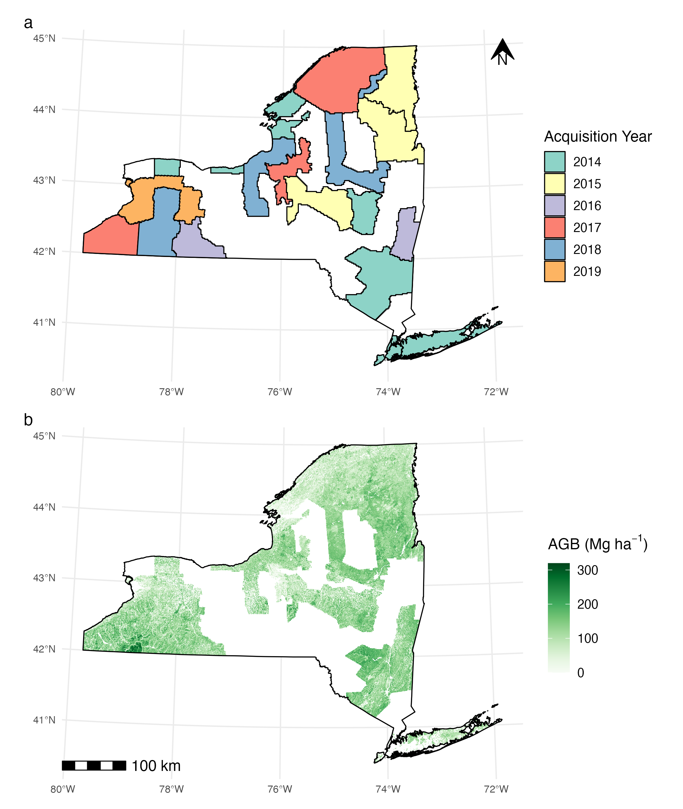
Figure 2: LiDAR-based AGB reference data. a) Spatial coverages of LiDAR collections colored by year of acquisition. b) Spatiotemporal patchwork of LiDAR-based AGB predictions sampled for reference data.

2.5 Landsat and auxiliary data

We produced a set of 16 annual Landsat-derived predictors by processing Landsat collection 1 data (C1, USGS (2018)) in Google Earth Engine (GEE, Gorelick et al. (2017)). We followed the processing framework described in Michael J. Mahoney et al. (2022), relying on growing-season medoid composites processed with coefficients from Roy et al. (2016) and the Landtrendr implementation in GEE (hereafter LT-GEE) to provide a continuous, and smoothed, 30-year time series of pixel-level metrics describing surface conditions and disturbance history (Kennedy, Yang, and Cohen 2010; Kennedy, Yang, et al. 2018). All spectral indices and their respective deltas computed with a 1-year lag (Hudak et al. 2020) were fit to Normalized Burn Ratio (NBR) temporally segmented vertices (Kennedy, Yang, et al. 2018). We computed the normalized burn ratio (NBR; Kauth and Thomas (1976)), tasseled-cap wetness, brightness, and greenness (TCW, TCB, TCG; Cocke, Fulé, and Crouse (2005)), normalized difference vegetation index (NDVI; Kriegler et al. (1969)), simple ratio (SR; Jordan (1969)), and modified simple ratio (MSR; Chen (1996)) using the ‘awesome-spectral-indices’ javascript library for GEE (Montero et al. 2022). The disturbance metrics were processed with a separate NBR segmentation using LT-GEE parameters designed to be more sensitive to the timing of discrete disturbance events (Kennedy, Yang, et al. 2018). We chose to use NBR to process all other LT-GEE-derived predictors, providing disturbance history and temporal break-points to which all other indices were fit, since it has been demonstrated to best represent disturbance events (Kennedy, Yang, and Cohen 2010). Supplementary Materials 1 provides additional information on the LT-GEE parameters used here.

We also included the annual primary and secondary land cover classification predictions from United States Geological Survey’s Land Change Monitoring, Assessment, and Projection (LCMAP) version 1.2 (Brown et al. 2020; Zhu and Woodcock 2014). Further, a set of steady-state ancillary predictors was included to represent geospatial variation in climate, topography, ecology, and landcover (Kennedy, Ohmann, et al. 2018). These predictors included precipitation and temperature 30 year normals derived from PRISM Climate Group data (PRISM Climate Group 2022), elevation, aspect, slope, and a topographic wetness index derived from a 30 m digital elevation model (Michael J. Mahoney, Beier, and Ackerman 2022; U.S. Geological Survey 2019; Beven and Kirkby 1979), a global canopy height map representing 2005 conditions (Simard et al. 2011; Hudak et al. 2020), distance (m) to nearest area and line water identified by the US Census Bureau (Walker 2022; US Census Bureau 2013), National Wetland Inventory classifications developed by the Fish and Wildlife Services (FWS) (FWS 2022; Wilen and Bates 1995), and the Environmental Protection Agency’s (EPA) level 4 ecozones (Omernik and Griffith 2014; CEC 1997). Where individual EPA level 4 ecozones did not cover $\geq$ 2% of the state they were aggregated to their level 3 ecozone, and if this aggregation did not cover $\geq$ 2% of the state these ecozones were set to “other”. All categorical variables (LCMAP, ecozones, wetlands) were encoded as boolean indicator variables.

Each of the 29 predictor layers (Table 2) were projected to match Landsat 30 m pixel geometries. The raster stacks of predictors were clipped and aggregated (weighted average) at the constructed FIA plot polygons (Section 2.3), and were also overlaid with the sampled LiDAR-based AGB predictions (Section 2.4), creating two distinct sets of data for model training based on the same set of predictors. The exactextractr (Daniel Baston 2022) and terra (Hijmans 2022) packages for the R (R Core Team 2021) programming language were used to compile the training datasets.

Table 2: Definitions of predictors used for model fitting.

Group	Predictor	Definition
	TCB, TCW, TCG	Tassled cap brightness, wetness, and greenness, with noise removed using LT-GEE
	NBR	Normalized burn ratio with noise removed using LT-GEE
	NDVI	Normalized difference vegetation index with noise removed using LT-GEE
	SR	Simple ratio with noise removed using LT-GEE
Spectral indices	MSR	Modified simple ratio with noise removed using LT-GEE
Delta	Delta_*	Change computed with 1 year lag for all predictors in the ’Spectral indices’ group
Disturbance	YOD, MAG	Year of most recent disturbance and associated magnitude of NBR change, as identified using an NBR segmentation in LT-GEE (1985-2019)
	CHM	Global canopy height model reflecting 2005 conditions (Simard 2011), downsampled from 1 km to 30 m resolution
	ECOZONE	EPA level 4 ecozones. Aggregated to level 3 if level 4 areas < 2% of the state. Set to ’other’ if level 3 aggregation < 2% of state.
	WETLAND	Wetland classification codes from the FWS National Wetlands Inventory
Ecological	DIST_TO_WATER	Distance in meters to nearest TIGER/Line Shapefile water from the US Census Bureau
Climate	PRECIP, TMAX, TMIN	30-year normals for precipitation, maximum temperature, and minimum temperature, derived from annual PRISM climate models
Topographic	ASPECT, ELEVATION, SLOPE, TWI	Aspect, elevation, slope, and topographic wetness index derived from a 30-meter digital elevation model
Landcover	LCPRI, LCSEC	LCMAP primary and secondary land cover classifications

2.6 Model development

We developed three distinct modeling approaches using a standard training framework. The direct approach involved training models on a random 80% partition of the model dataset derived from FIA field data (Section 2.3), and the indirect approach involved training models on a random 80% partition of the sample of LiDAR-based AGB predictions (Section 2.4). We developed separate sets of ML models for both approaches and combined each set in a stacked ensemble to better reflect model selection uncertainty (Wintle et al. 2003) and to reduce the generalization error of our component models (Wolpert 1992). The third approach was an ensemble combining predictions from the direct and indirect ensemble models in a simple average, as model averaging has been demonstrated to improve upon individual predictions where data is noisy and the relationships between predictors and responses are complex and largely unknown (Wolpert 1992; Dormann et al. 2018). For all three approaches, we used the 20% test partitions to assess model performance against each respective dataset and iterate with various predictors and model forms.

Both the direct and indirect approaches used all 29 predictors described in Section 2.5, while the ensemble was developed with only predictions from these models. Both the direct and indirect approaches combined a random forest, as implemented in the ranger R package (Breiman 2001; Wright and Ziegler 2017) and a stochastic gradient boosting machine (GBM) as implemented in the lightgbm R package (Friedman 2002; Ke et al. 2017; Shi et al. 2022). The direct approach also incorporated a support vector machine (SVM) as implemented in the kernlab R package (Cortes and Vapnik 1995; Karatzoglou et al. 2004). SVM training time scales between quadratic and cubic with respect to training observations (Bottou and Lin 2007) and thus was not computationally feasible to implement our indirect approach with 16,000 training points.

Each of the component ML models were tuned using the 80% training partition described above and an iterative grid search, starting by testing wide ranges of hyperparameters using five-fold cross validation and then narrowing down to only the most performant combinations over several iterations. Models then used the most accurate sets of hyperparameters in all other analyses. The selected hyperparameters for each component model and the coefficients in the linear regression ensembles are available in Supplementary Materials 2. For each of the n observation in the training dataset, all component models were fit, using their optimal hyperparameters, with n-1 observations. Predictions for each component model were made for the nth (left out) observation. A linear regression model was used to estimate AGB as a function of these leave-one-out predictions, combining the component ML models in a linear regression ensemble as follows:

$$\hypertarget{eq-ensemble}{}{\operatorname{AGB}=\beta_{0}+\beta_{1}\cdot P_{1}+\ldots+\beta_{n}\cdot P_{n}}$$ (1)

where $\beta_{*}$ are coefficients estimated through ordinary least squares regression, and $P_{*}$ are the respective component model predictions. At an abstract level the direct approach was constructed as follows:

$$\hypertarget{eq-direct}{}{\operatorname{AGB}=ensemble(RF,SVM,LGB)}$$ (2)

where $ensemble$ represents Equation 1, and $RF$, $SVM$, and $GBM$ would be substituted for the $P_{*}$ variables in Equation 1. The indirect approach was constructed as follows:

$$\hypertarget{eq-indirect}{}{\operatorname{AGB}=ensemble(RF,LGB)}$$ (3)

and the overarching ensemble was constructed as follows:

$$\hypertarget{eq-big-ensemble}{}{\operatorname{AGB}=\frac{ensemble(RF_{direct},SVM_{direct},LGB_{direct})+ensemble(RF_{indirect},LGB_{indirect})}{2}}$$ (4)

2.7 AGB mapping and postprocessing

The linear model ensembles for the direct and indirect approaches, as well as the overarching average ensemble, were used to make predictions for all 30 m pixels across the state. With recognition that our predictions are best suited to areas populated by woody biomass, we overlaid our predictions with the LCMAP version 1.2 primary landcover classification product (Brown et al. 2020; Zhu and Woodcock 2014), which has a reported overall accuracy of 77.4% in the Eastern United States for the years 1985-2018 (Pengra et al. 2020). LCMAP data shared identical pixel geometries with our AGB maps and its annual resolution allowed for temporal alignment with each individual year of mapping. We masked our AGB prediction surfaces to remove developed, cropland, water, and barren pixels and then tabulated AGB by the three remaining vegetated LCMAP classes of tree cover, grass/shrub, and wetland.

2.8 Map agreement assessment

We assessed the agreement between our AGB maps and FIA reference data following approaches prescribed by Riemann et al. (2010) and Menlove and Healey (2020). The former evaluated agreement across a range of scales and accounts for the mismatch in spatial support between map aggregate estimates (many pixels) and FIA aggregate estimates (few plots) by only extracting pixels coincident with FIA plots. The latter compared FIA-derived AGB estimates – which have been adjusted for forest cover within, and area-extrapolated to, hexagon map units – to zonal averages of our mapped AGB.

Following Riemann et al. (2010) we compared our AGB prediction surfaces from each of the three modeling approaches to the map assessment dataset (Section 2.3). Comparisons were made at both the plot-to-pixel scale and within variably-sized hexagons with distances between centroids ranging from 20 km (34,641 ha) to 50 km (216,506 ha). Since the plot inventories spanned multiple years (2007, 2012, 2018, 2019) we extracted predictions from only those map surfaces that were temporally aligned with the specific plot inventories in our dataset. We then pooled this data together, producing a temporally generalized accuracy assessment. As an extension of the Riemann et al. (2010) methodology we assessed the spatial patterns of prediction error by summarizing the plot-to-pixel residuals and FIA reference data distributions within hexagon units with centroids spaced 50 km apart. We also grouped plot-to-pixel results by the majority LCMAP classification at each plot, to demonstrate the level of agreement across vegetated landcover classes.

Following the Menlove and Healey (2020) approach, we compared the average of our masked predictions, weighted by the proportion of each pixel intersecting a given hexagon, to a set of FIA-derived estimates for 64,000 ha hexagons representing FIA’s finest acceptable scale for the most recent inventory cycle in NYS (2013–2019). We used 2016 AGB maps from each approach for this comparison since 2016 sits in the center of the time period that is represented in the Menlove and Healey (2020) data. As recommended, we accounted for differences in forest definitions between the FIA estimates and our mapped estimates by dividing FIA estimates by the proportion of vegetated (based on LCMAP tree cover, grass/shrub, wetland) area within each hexagon. Lastly, we limited this comparison to only hexagons with a majority area falling inside NYS boundaries.

Assessment metrics included mean absolute error in Mg ha^-1 (MAE), percent MAE relative to mean reference AGB (% MAE), root-mean-squared error in Mg ha^-1 (RMSE), percent RMSE relative to mean reference AGB (% RMSE), mean error in Mg ha^-1 (ME), and the coefficient of determination ($R^{2}$). Equations and formulas for each metric and the associated estimates of standard errors are provided in Supplementary Materials 3. The exactextractr (Daniel Baston 2022), sf (Pebesma 2018), and terra (Hijmans 2022) packages in the R programming language (R Core Team 2021) were used to conduct all analyses described here.

2.9 Qualitative comparisons of fine spatial patterns

We also visually compared mapped predictions for each modeling approach in and around Huntington Wildlife Forest (HWF), a 6,000 ha forested area in Newcomb, NYS containing both reserves and areas of active management and where our team has developed a familiarity with the landscape through in situ and remote observations alike. Though limited to a small fraction of the statewide context, this comparison aimed to qualitatively assess relative strengths and weaknesses in characterizing fine spatial patterns of AGB density across various management regimes and landscape conditions. We conducted pair-wise raster subtraction to produce surfaces that highlighted areas of disagreement across modeling approaches and used both a 1 m LiDAR-derived canopy height model (CHM; Atlantic Inc (2015)) as well as 0.5 m natural color imagery from the National Aerial Imagery Program (NAIP; Earth Resources Observation And Science (EROS) Center (2017)) for additional qualitative reference information. The CHM and the NAIP imagery reflected conditions in 2015, and so 2015 AGB prediction surfaces from each modeling approach were compared.

3 Results

3.1 Annual aboveground biomass maps

We produced 30 years (1990-2019) of statewide AGB maps at a 30 m resolution using each of the three modeling approaches. Statewide AGB averages for each of the three modeling approaches increased steadily over the time period for each of the included LCMAP classifications (Figure 3). However, in agreement with its higher saturation threshold (Section 3.2), the indirect approach produced significantly larger averages than both the direct and the ensemble approaches (Figure 3). Around 2006, all three models produced small decreases in the statewide average for tree cover classified pixels; this corresponds with the timing of large-scale insect outbreaks in the Northeast (2005-2007, Kosiba et al. (2018)), and specifically a forest tent caterpillar (Malacosoma disstria) defoliation event that affected roughly 1.2 million acres of land in NYS (USFS 2006). While defoliation alone does not necessarily result in AGB loss, our models’ reliance on spectral information precluded them from making the distinction between canopy-specific changes and structural changes.

A full time timeseries raster subtraction (2019 AGB - 1990 AGB) using the ensemble predictions reflected these annual trends, with increases in AGB dominating the map (Figure 4). The 30-year stock-change map also featured patterns of AGB change driven by anthropogenic impacts and cadastral boundaries contrasted with those that can be attributed to otherwise natural processes. Specifically, the stock-change map highlighted a mosaic of working forests and Adirondack Forest Preserve land and the varying spatial patterns and magnitudes of change accompanying these distinct land uses (Figure 4 b), distinguished patchy AGB losses within privately held lands to the west of the Allegany river against subtle AGB gain and relative stability within Allegany State Park to the east of the river (Figure 4 c), and revealed a band of forest growth that runs north to south along the border of the Catskill Forest Preserve (Figure 4 d).

At the stand scale, where we have landowner-provided management records in Northern NYS, our annual maps accurately captured the timing, severity, and subsequent recovery (regeneration) from harvest activities in working forests (Figure 5). Looking in particular at the clearcut harvests in Figure 5 and the residual AGB within the boundaries of these polygons, we note that the spatial management records we have are best approximations of harvest prescriptions and may not reflect the true extent of harvest activity. Likewise, disturbances outside these harvest polygons were captured in our mapped predictions (note western portion of Figure 5 beginning in 2015) and in this instance can be attributed to harvest events that were simply not included in the records provided by the landowner.

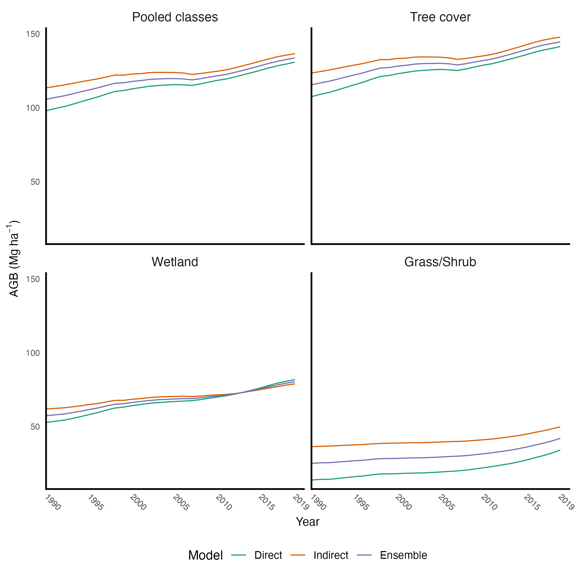
Figure 3: Annual statewide summaries (average AGB) for each modeling approach by LCMAP class.

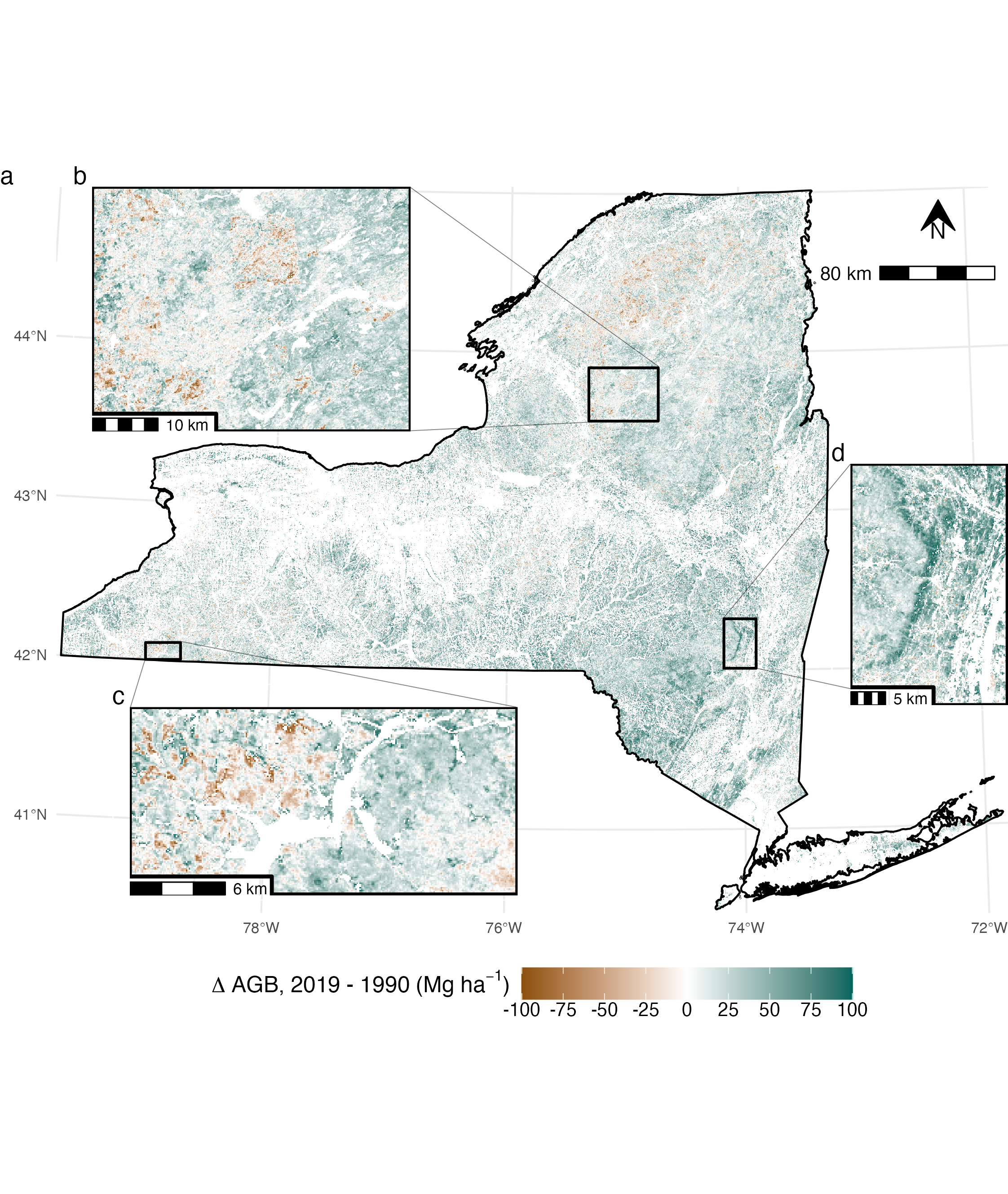
Figure 4: New York State (USA) AGB difference map (2019 AGB - 1990 AGB) with predictions from the ensemble model. a) Statewide scale. b) A mosaic of working forests and Adirondack Forest Preserve land south of Stillwater Reservoir, NYS. c) Allegany River area with a portion of Allegany State Park to the east of the river. d) Forest growth along the border of the Catskill Forest Preserve. Values are capped at $\pm$ 100 Mg ha^-1 for display.

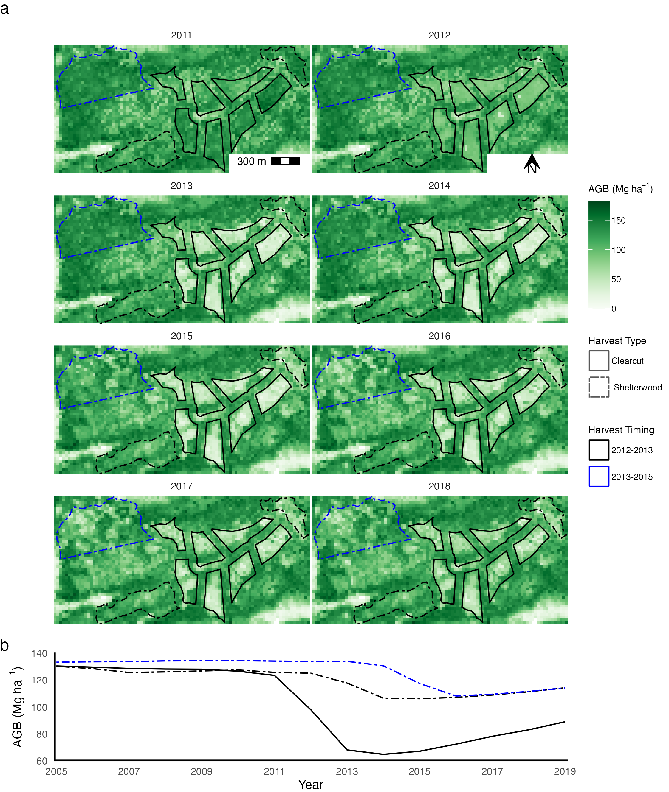
Figure 5: Quantifying AGB changes due to harvests and subsequent regeneration in Northern New York State (USA). a) Annual AGB predictions from the ensemble model for selected years overlaid with harvest records symbolized by documented harvest type and timing. b) Annual area-level summaries of mapped predictions (average AGB) for harvest polygons grouped by harvest type and timing with trajectory symbology corresponding to polygon symbology in a).

3.2 Map agreement

Although differences in estimated accuracy metrics were nominal among our three modeling approaches, the ensemble model was most accurate (Table 3). The indirect approach on the other hand was least accurate by these metrics, likely due to the additive effects of pixel-level error in the initial LiDAR-AGB predictions (Johnson et al. 2022). We observed improved agreement between mapped predictions and FIA estimates as the aggregation unit size increased for all three modeling approaches, with % MAE decreasing from 34.1 to 19.46% for the direct approach, from 35.69 to 20.23% for the indirect approach, and from 33.88 to 19.23% for the ensemble approach (Table 3). Similar patterns of increasing agreement were exhibited for MAE, RMSE, %RMSE, and R², but ME estimates were mostly stable and positive across all scales of aggregation.

All three models tended to overpredict on zero and near-zero AGB reference observations, particularly at the plot:pixel and 20 km scales of comparison (Figure 6), which resulted in positive and significant ME estimates (Table 3). Many of these overpredictions can be explained by our reliance on tree-based models (RF, GBM) whose predictions are the average values within terminal nodes (Baccini et al. 2008; Urbazaev et al. 2018). However, these overpredictions might also have been due to structural zeroes in our map assessment dataset, where FIA AGB was assumed to be zero but is actually not measured due to FIA’s strict forest definition (Section 2.3; Johnson et al. (2022)). Large relative errors in FIA plots classified as grass/shrub provided further evidence of the impact of forest definition discrepancies on our map agreement results (Table 4). Unfortunately, we have had no means to identify plots containing structural zeroes without additional data, and could not separate them from plots with otherwise real overpredictions and errors.

Underprediction on the largest reference observations (i.e. saturation), a common issue when modeling forest structure with optical imagery (Lu 2005; Duncanson, Niemann, and Wulder 2010), was evident for all three modeling approaches but to varying degrees (Figure 6). The direct approach saturated first, failing to predict beyond 204 Mg ha^-1, whereas the indirect approach was the best in this regard, predicting up to 289 Mg ha^-1 and leaving only 1% of the reference data beyond its ceiling. In general, patterns of over and underprediction diminished and systematic agreement improved at larger scales of aggregation as evidenced by the convergence of GMFR and 1:1 lines for all models (Figure 6). The indirect approach yielded the best systematic agreement (GMFR vs 1:1) across all scales despite being least accurate in terms of the estimated metrics (Figure 6; Table 3).

Map comparisons with the FIA’s small area estimates (Menlove and Healey (2020)) similarly demonstrated both patterns of over and under prediction on the extremes of reference AGB distributions, as well as the effects of saturation for each of the three modeling approaches (Supplementary Materials 4). Despite consistently underpredicting relative to the Menlove and Healey (2020) estimates, the direct approach yielded more estimates within the provided 95% confidence intervals (90.31%) as compared to the ensemble (88.27%) and indirect (85.2%) approaches. Likewise, local errors (over and underprediction) were more related to the amount of reference AGB within each hexagonal unit rather than spatial or regional patterns when plot-to-pixel residuals were mapped (Supplementary Materials 4).

Tree cover agreement for each model (Table 4) largely matched the overall plot-to-pixel agreement in Table 3, because the vast majority of map assessment plots fell within this classification. Map agreement was worse for the fewer number of wetland and grass/shrub classified plots, with ME estimates indicating significant overprediction in grass/shrub classified plots and underprediction in wetland classified plots (Table 4). This discrepancy in agreement among vegetated classes can likely be attributed to the varying degrees to which each landcover classification was represented in our reference datasets and the mismatch between our LCMAP-defined vegetation mask (Section 2.7) and the strict forest definition used by FIA (Section 2.3).

Table 3: Map agreement results for select scales. RMSE, MAE, ME in Mg ha^-1. Scale = distance between hexagon centroids in km; PPH = plots per hexagon; n = number of comparison units (plots or hexagons). All accuracy metrics as defined in Supplementary Materials 3. Standard errors in parentheses with minimum capped at 0.01.

Scale	n	PPH	Model	% MAE	MAE	% RMSE	RMSE	ME	R²
			Direct	34.10	41.20 (1.38)	43.29	52.31 (3.06)	4.83 (2.23)	0.38 (0.01)
			Indirect	35.69	43.13 (1.44)	45.30	54.73 (3.14)	11.15 (2.30)	0.32 (0.01)
Plot:Pixel	545		Ensemble	33.88	40.94 (1.36)	42.84	51.76 (2.98)	7.99 (2.19)	0.39 (0.01)
			Direct	29.17	35.53 (1.69)	37.81	46.06 (4.19)	3.42 (2.65)	0.40 (0.01)
			Indirect	31.51	38.39 (1.71)	39.80	48.48 (3.92)	9.22 (2.74)	0.33 (0.01)
20 km	302	1.8	Ensemble	29.57	36.02 (1.64)	37.65	45.86 (4.21)	6.32 (2.62)	0.40 (0.01)
			Direct	25.35	30.76 (1.87)	32.41	39.32 (6.12)	3.66 (2.99)	0.37 (0.01)
			Indirect	27.40	33.25 (1.86)	33.97	41.21 (5.34)	10.03 (3.06)	0.30 (0.01)
30 km	172	3.17	Ensemble	25.79	31.30 (1.76)	32.02	38.86 (5.01)	6.85 (2.93)	0.38 (0.01)
			Direct	19.46	23.85 (2.70)	26.97	33.05 (12.80)	2.58 (3.88)	0.43 (0.01)
			Indirect	20.23	24.80 (2.39)	26.14	32.04 (8.54)	9.46 (3.61)	0.46 (0.01)
50 km	73	7.47	Ensemble	19.23	23.57 (2.39)	25.38	31.10 (10.31)	6.02 (3.60)	0.49 (0.01)

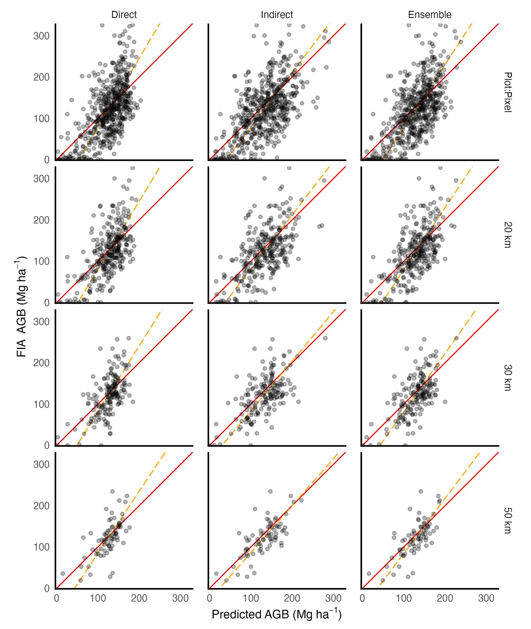
Figure 6: Comparison of mapped AGB to FIA estimated AGB across selected scales represented by distances between hexagon centroids (plot:pixel, 10 km, 25 km, and 50 km). Geometric mean functional relationship (GMFR) trend line shown with dashed (orange) line, and 1:1 line shown with solid (red) line

Table 4: Map agreement at the plot to pixel scale, grouped by LCMAP classification. RMSE. MAE, ME in Mg ha^-1. n = number of plots. All accuracy metrics as defined in Supplementary Materials 3. Standard errors in parentheses with values capped at 0.01 and 1.00.

LCMAP	n	Model	% MAE	MAE	% RMSE	RMSE	ME	R²
		Direct	87.58	34.07 (7.50)	111.81	43.49 (66.44)	3.76 (12.02)	0.41 (1.00)
		Indirect	101.20	39.36 (10.95)	143.30	55.74 (217.09)	33.85 (12.28)	0.03 (1.00)
Grass/Shrub	14	Ensemble	93.92	36.53 (6.65)	112.34	43.69 (51.15)	18.80 (10.94)	0.40 (1.00)
		Direct	40.19	34.56 (4.34)	55.15	47.43 (28.20)	-9.21 (6.22)	0.40 (0.01)
		Indirect	43.47	37.38 (4.26)	57.12	49.12 (29.95)	-10.29 (6.42)	0.35 (0.02)
Wetland	57	Ensemble	40.87	35.15 (4.22)	54.94	47.24 (31.20)	-9.75 (6.18)	0.40 (0.01)
		Direct	33.13	42.21 (1.48)	41.67	53.10 (3.44)	6.55 (2.42)	0.31 (0.01)
		Indirect	34.47	43.93 (1.55)	43.42	55.34 (3.46)	13.06 (2.47)	0.26 (0.01)
Tree cover	474	Ensemble	32.78	41.77 (1.46)	41.19	52.50 (3.23)	9.80 (2.37)	0.33 (0.01)

3.3 Qualitative comparisons of fine spatial patterns

Within Huntington Wildlife Forest (HWF), in the forest preserve land to the north of HWF (High Peaks Wilderness; Pataki and Cahill (1999)), and in the working forest to the southwest of HWF, the indirect AGB map best represented known patterns across the landscape and contained the most spatial heterogeneity relative to the other two approaches (Figure 7). This was most evident where the largest discrepancies between maps were present in the northeast and the northwest corners of the area. In the northeast corner, where conifer-dominated wetlands (NAIP Figure 7) contained some of the tallest vegetation in the area (CHM Figure 7), the indirect approach produced large biomass predictions ($\geq$ 225 Mg ha^-1) in agreement with these landscape features. In the northwest corner of the map, where high-elevation spruce-fir forests are present, the indirect approach produced correspondingly small AGB predictions whereas the direct approach was unable to distinguish these conditions from the rest of the landscape. By definition, the ensemble map represented a blend of characteristics from the direct and indirect maps in terms of both fine spatial patterns and magnitudes of predictions.

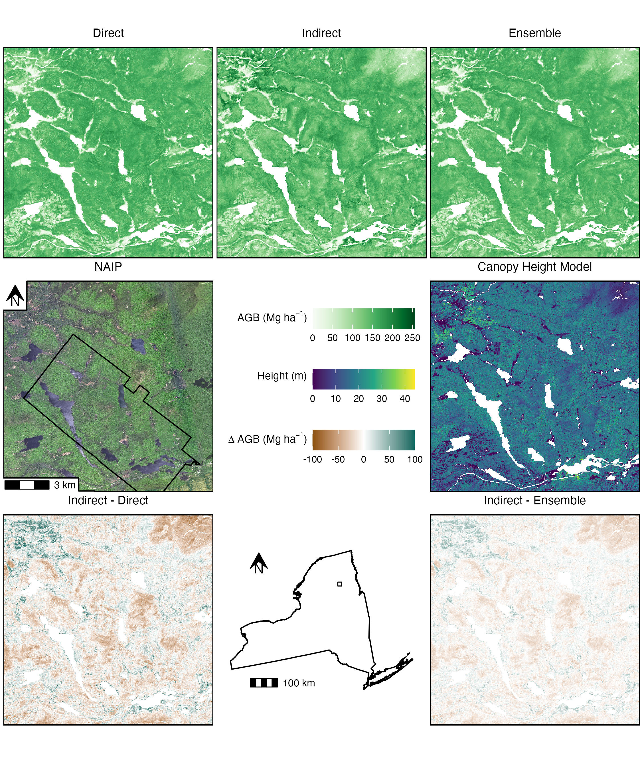
Figure 7: A qualitative comparison of maps from each modeling approach within Huntington Wildlife Forest (boundary mapped with black box in NAIP panel) and the surrounding area in Newcomb, New York (full area extent mapped with black box in New York State panel). Pair-wise raster subtractions (values capped at $\pm$ 100 Mg ha^-1 for display) highlight spatial patterns and magnitudes of differences between model predictions. Ensemble - Direct not shown because it duplicates Indirect - Ensemble. A 1 m LiDAR-derived canopy height model and 0.5 m natural color National Aerial Imagery Program (NAIP) orthophotography included for additional reference information. All surfaces represent conditions in 2015.

4 Discussion

In this study we combined temporally smoothed, segmented, and gap-filled Landsat imagery with a sample of LiDAR-based aboveground biomass (AGB) predictions and a set of the USDA’s Forest Inventory and Analysis (FIA) field plots to produce annual wall-to-wall maps of AGB for New York State (NYS), USA. To this end, we developed three separate modeling approaches including direct, indirect, and ensemble approaches. Overall, we found that all three modeling approaches performed similarly, indicating that each approach could be satisfactory on its own, yet tradeoffs were evident relating to model complexity, map accuracy, saturation, and representation of fine spatial patterns. Comparisons to existing studies with similar goals, but in temperate regions with different disturbance and management regimes, indicated that the basic methods herein can be leveraged to track forest biomass dynamics across ecological domains and within working forests regardless of the dominating forestry practices. The maps produced from each modeling approach offer valuable insights into the spatiotemporal patterns of forest structure, development, disturbance, and change over 30 years and can serve as inputs for a variety of applications related to map-based stock-change assessments, screening or prioritizing forest parcels for enrollment in nature-based climate programs, and future monitoring, reporting, and verification (MRV) systems across NYS.

4.1 Tradeoffs among modeling approaches

There was no single winner among the three modeling approaches, but rather each offered a set of benefits that can appeal to different project-specific constraints and goals. Overall, the ensemble approach produced the most accurate maps (Table 3) which combined characteristics from the direct and indirect approaches in terms of fine-scale pattern representation and model saturation. Though it was the most complex of the three approaches, it simultaneously mitigated limitations and leveraged strengths associated with the plot-based (Section 2.3) and lidar-based (Section 2.4) training datasets. These results provide general support for model ensembling in ecological applications where data are noisy and natural variability is a significant source of error (Dormann et al. 2018).

By definition the direct approach was most parsimonious with only one stage of modeling and the smallest investment of time and effort required to produce AGB map products. The indirect and ensemble approaches required the computationally demanding management and analysis of terabytes of LiDAR data (Johnson et al. 2022), though that effort could be reduced if LiDAR strips or samples were used in lieu of wall to wall mapping (Wulder et al. 2012; Matasci et al. 2018; Urbazaev et al. 2018). Additionally, increased complexity embedded in the indirect and ensemble models makes estimating prediction uncertainty more challenging than for the direct approach (Saarela et al. 2016).

The indirect approach was least impacted by saturation, resulting in the best systematic agreement with FIA reference data across all scales (Figure 6). With only 1% of reference AGB plots beyond the indirect model’s prediction ceiling, this approach was best suited to track continued growth in mature forest stands. This feature would be especially important in NYS and the broader region where historical land-use dynamics indicate that the majority of forest stands have either reached or are approaching maturity (Section 2.2). Failure to accurately quantify AGB in these stands will lead to significant underestimation of carbon storage and sequestration, at both local and statewide scales. Further, we found that the indirect approach produced maps that best aligned with our knowledge of local forest conditions and best represented fine-scaled features on the landscape (Figure 7). The strengths of the indirect model can be attributed to the much larger sample of reference data, and in theory the greater coverage of both the AGB distribution and the landscape conditions in NYS, acquired from broad-scale LiDAR-based AGB maps (Section 2.4).

4.2 Comparison to existing studies

Comparisons of model performance and map agreement across studies should be made with caution, as landscapes, data collection protocols, remotely sensed data products, and AGB distributions can differ widely and have large impacts on resulting agreement metrics. However, we do so here in a relative fashion to situate the success of our approaches among existing studies with similar goals. Kennedy, Ohmann, et al. (2018), Hudak et al. (2020), and Matasci et al. (2018) each leveraged Landsat time series data to map AGB annually at a 30 m resolution across the following regions and time periods (respectively): Western Cascades province of Oregon and Northern California, 2000-2016; Washington, Oregon, Idaho, and Montana, 1990-2012; Canada’s forest-dominated ecosystems, 1984-2016. Kennedy, Ohmann, et al. (2018) used direct modeling only, yielding an RMSE of ~103 Mg ha^-1 against model training plots with a wide range of AGB values (0-1000 Mg ha^-1), while Hudak et al. (2020) and Matasci et al. (2018) exclusively used indirect modeling, yielding 64% RMSE against independent FIA plots, and 66% RMSE against LiDAR-based AGB predictions respectively. Although these kinds of direct comparisons have caveats, they signify that similar methods relying on Landsat time series imagery to characterize forest dynamics are applicable in multiple domains – from conifer-dominated western US and Canadian forests with even-aged disturbance regimes (Kennedy, Ohmann, et al. 2018; White et al. 2017), to northern hardwoods and mixed forests of the eastern US with mostly uneven-aged disturbance regimes (Section 2.2). This capacity to track changes in forests with varying disturbance patterns and management systems is needed to ensure that all working forest landowners and landscapes are treated accurately and fairly within large-scale carbon accounting frameworks (Desrochers et al. 2022).

4.3 Applications for annual AGB maps

Our rigorously evaluated map products have a range of applications where knowledge of the spatiotemporal patterns of forest biomass (and by extension, forest carbon pools) is needed. Most immediately, given our extensive use of FIA plot-level information for model development (Section 2.3, Section 2.4) and map assessment (Section 2.8), our annual maps provide a translation of FIA information to inputs for spatially explicit stock-change accounting methods. Such a map-based framework offers the capability to summarize stock changes and rates of sequestration following FIA’s accounting approach, but with the additional flexibility to do so for arbitrary units of area within NYS for any time window in the 30 year period (Figure 4). This increased resolution enabled the identification of AGB losses and gains with distinct spatiotemporal signatures attributed to conservation, regulation, and ownership patterns across the landscape (Figure 4 b, c, d). While sample-based stock-change approaches will capture these outcomes in aggregate, our maps can more precisely identify where, when, and how both human and natural processes are impacting forest carbon stocks across the landscape.

Although modeled data should not supersede direct measurements, inventories, or boots-on-the-ground knowledge, the historical perspective provided by our maps allows us to fill in gaps where management records or forest inventory data are not available (Figure 5). The availability of both past management information and historical AGB or carbon stock information opens the door to a host of opportunities to quantify the outcomes of various management regimes (Kaarakka et al. 2021; Patton et al. 2022). Further, the burden of proving additionality for enrollment in carbon offset programs hinges on establishing credible business-as-usual baselines that are impossible to produce without historical data (Gillenwater et al. 2007). Map datasets such as those developed here can fill this gap for both potential enrollees and program managers alike, minimizing many of the otherwise prohibitive up-front costs and requirements (Charnley, Diaz, and Gosnell 2010; Kerchner and Keeton 2015). More broadly, these historical datasets can provide baselines for better understanding present and future forest conditions in response to multiple drivers of change, including a rapidly changing climate (Cohen et al. 2016; White et al. 2017).

Because we have primarily relied on federally funded and publicly available data sources, as well as open source software and tools, we have the flexibility to leverage the same methods developed for this historical context to fulfill ongoing monitoring (MRV) needs. Our modeling workflow needs only to be updated with annual Landsat imagery and FIA inventories along with opportunistic additions of LiDAR collections (Sugarbaker et al. 2014, 2017) to provide a highly cost-effective landscape monitoring framework that is broadly reproducible and extensible. This approach could be further enhanced by integrating new streams of information that have the potential to improve predictive accuracy relative to models trained with Landsat alone (e.g. ESA’s Biomass mission – Quegan et al. (2019), NASA’s GEDI mission – Dubayah et al. (2014)).

Up-to-date maps of AGB and carbon stocks will allow decision-makers to prioritize parcels for both protection via purchase of fee titles or conservation easements, as well as for enrollment in improved forest management programs and carbon markets (Merenlender et al. 2004; Malmsheimer et al. 2008; Kelly, Germain, and Stehman 2015; Kerchner and Keeton 2015). Similarly, timely annual AGB maps can support wall-to-wall MRV and harvest monitoring, not necessarily in lieu of essential field visits, but as a means to screen those parcels which are likely in compliance from those which require a closer look (Gillenwater et al. 2007). Not only would monitoring costs be significantly reduced under such a system, likely lowering financial break-even thresholds for potential projects (Charnley, Diaz, and Gosnell 2010; Kerchner and Keeton 2015), but strictly random site visits would also be rendered dispensable when a regular census of properties or land holdings is otherwise unfeasible. Beyond annual monitoring, fine-resolution AGB trajectories derived from our 30 years of maps could inform timeseries forecasting and landscape simulation studies that aim to predict the carbon consequences of various policy and management scenarios (MacLean et al. 2021).

5 Conclusion

Fine-resolution maps of historical forest dynamics can serve as inputs to spatially explicit stock-change accounting frameworks that offer critical information for projecting carbon outcomes of land stewardship decisions at parcel to landscape scales. There is an essential need for methods that can deliver these historical datasets in the near term and that offer reproducible, consistent, and widely applicable data products. We have demonstrated three model-based approaches leveraging open source data, software, and tools to predict AGB annually, at a 30 m resolution, across New York State (NYS) for the past three decades (1990-2019). Our results show that each of the three approaches provide valid outputs and offer unique benefits relative to each other, thus offering a set of options for NYS where forests are expected to contribute substantially as carbon sinks towards achieving a net-zero carbon economy by 2050. More broadly, the map products produced here can help managers and decision-makers maximize the role forested landscapes will play in natural climate solutions and policies.

6 Acknowledgements

We would like to thank the USDA FIA program for their data sharing and cooperation, the Dutch Pension Fund and F & W Forest Management, LLC for sharing management records, the NYS GPO for compiling and serving LiDAR data, and the NYS Department of Environmental Conservation, Office of Climate Change for funding support. We would also like to thank Grant M. Domke, Stephen V. Stehman, and Eddie Bevilacqua for their support and guidance throughout this project.

References

reAbdalati, Waleed, H. Jay Zwally, Robert Bindschadler, Bea Csatho, Sinead Louise Farrell, Helen Amanda Fricker, David Harding, et al. 2010. “The ICESat-2 Laser Altimetry Mission.” Proceedings of the IEEE 98 (5): 735–51. https://doi.org/10.1109/jproc.2009.2034765.

preAtlantic Inc. 2015. “NY_WarrenWashingtonEssex_Spring2015.” ftp://ftp.gis.ny.gov/elevation/LIDAR/.

preBaccini, A, N Laporte, S J Goetz, M Sun, and H Dong. 2008. “A First Map of Tropical Africa’s Above-Ground Biomass Derived from Satellite Imagery.” Environmental Research Letters 3 (4): 045011. https://doi.org/10.1088/1748-9326/3/4/045011.

preBanskota, Asim, Nilam Kayastha, Michael J. Falkowski, Michael A. Wulder, Robert E. Froese, and Joanne C. White. 2014. “Forest Monitoring Using Landsat Time Series Data: A Review.” Canadian Journal of Remote Sensing 40 (5): 362–84. https://doi.org/10.1080/07038992.2014.987376.

preBechtold, William A, and Paul L Patterson. 2005. The Enhanced Forest Inventory and Analysis Program–National Sampling Design and Estimation Procedures. Vol. 80. USDA Forest Service, Southern Research Station. https://doi.org/10.2737/SRS-GTR-80.

preBeven, Keith J., and Mike J. Kirkby. 1979. “A Physically Based, Variable Contributing Area Model of Basin Hydrology.” Hydrological Sciences Bulletin 24 (1): 43–69. https://doi.org/10.1080/02626667909491834.

preBottou, Léon, and Chih-Jen Lin. 2007. “Support Vector Machine Solvers.” Large Scale Kernel Machines 3 (1): 301–20. https://web2.qatar.cmu.edu/~gdicaro/10315-Fall19/additional/SVM-solvers.pdf.

preBreiman, Leo. 2001. “Random Forests.” Machine Learning 45 (1): 5–32. https://doi.org/10.1023/A:1010933404324.

preBrown, Jesslyn F., Heather J. Tollerud, Christopher P. Barber, Qiang Zhou, John L. Dwyer, James E. Vogelmann, Thomas R. Loveland, et al. 2020. “Lessons learned implementing an operational continuous United States national land change monitoring capability: The Land Change Monitoring, Assessment, and Projection (LCMAP) approach.” Remote Sensing of Environment 238: 111356. https://doi.org/10.1016/j.rse.2019.111356.

preBuendia, E, K Tanabe, A Kranjc, J Baasansuren, M Fukuda, S Ngarize, A Osako, Y Pyrozhenko, P Shermanau, and S Federici. 2019. “Refinement to the 2006 IPCC Guidelines for National Greenhouse Gas Inventories.” IPCC: Geneva, Switzerland 5: 194.

preCEC. 1997. Ecological Regions of North America: Toward a Common Perspective. Commission for Environmental Cooperation (Montréal, Québec).; Secretariat.

preCharnley, Susan, David Diaz, and Hannah Gosnell. 2010. “Mitigating Climate Change Through Small-Scale Forestry in the USA: Opportunities and Challenges.” Small-Scale Forestry 9 (4): 445–62. https://doi.org/10.1007/s11842-010-9135-x.

preChen, Jing M. 1996. “Evaluation of Vegetation Indices and a Modified Simple Ratio for Boreal Applications.” Canadian Journal of Remote Sensing 22 (3): 229–42. https://doi.org/10.1080/07038992.1996.10855178.

preCocke, Allison E., Peter Z. Fulé, and Joseph E. Crouse. 2005. “Comparison of Burn Severity Assessments Using Differenced Normalized Burn Ratio and Ground Data.” International Journal of Wildland Fire 14: 189–98. https://doi.org/10.1071/WF04010.

preCohen, Warren B., Zhiqiang Yang, Stephen V. Stehman, Todd A. Schroeder, David M. Bell, Jeffrey G. Masek, Chengquan Huang, and Garrett W. Meigs. 2016. “Forest Disturbance Across the Conterminous United States from 1985–2012: The Emerging Dominance of Forest Decline.” Forest Ecology and Management 360 (January): 242–52. https://doi.org/10.1016/j.foreco.2015.10.042.

preCooke, William H. 2000. “Forest/Non-Forest Stratification in Georgia with Landsat Thematic Mapper Data.” In McRoberts, Ronald e.; Reams, Gregory a.; van Deusen, Paul c., Eds. Proceedings of the First Annual Forest Inventory and Analysis Symposium; Gen. Tech. Rep. NC-213. St. Paul, MN: US Department of Agriculture, Forest Service, North Central Research Station: 28-30.

preCortes, Corinna, and Vladimir Vapnik. 1995. “Support-Vector Networks.” Machine Learning 20 (3): 273–97. https://doi.org/10.1007/bf00994018.

preDaniel Baston. 2022. Exactextractr: Fast Extraction from Raster Datasets Using Polygons. https://CRAN.R-project.org/package=exactextractr.

preDesrochers, Madeleine L, Wayne Tripp, Stephen Logan, Eddie Bevilacqua, Lucas Johnson, and Colin M Beier. 2022. “Ground-Truthing Forest Change Detection Algorithms in Working Forests of the US Northeast.” Journal of Forestry 120 (5): 575–87. https://doi.org/10.1093/jofore/fvab075.

preDormann, Carsten F., Justin M. Calabrese, Gurutzeta Guillera-Arroita, Eleni Matechou, Volker Bahn, Kamil Bartoń, Colin M. Beale, et al. 2018. “Model Averaging in Ecology: A Review of Bayesian, Information-Theoretic, and Tactical Approaches for Predictive Inference.” Ecological Monographs 88 (4): 485–504. https://doi.org/10.1002/ecm.1309.

preDubayah, Ralph, Scott J Goetz, James Bryan Blair, TE Fatoyinbo, Matthew Hansen, Sean P Healey, Michelle A Hofton, et al. 2014. “The Global Ecosystem Dynamics Investigation.” In AGU Fall Meeting Abstracts, 2014:U14A–07.

preDuncanson, LI, KO Niemann, and MA Wulder. 2010. “Integration of GLAS and Landsat TM Data for Aboveground Biomass Estimation.” Canadian Journal of Remote Sensing 36 (2): 129–41. https://doi.org/10.5589/m10-037.

preDyer, James M. 2006. “Revisiting the Deciduous Forests of Eastern North America.” BioScience 56 (4): 341–52. https://doi.org/10.1641/0006-3568(2006)56%5B341:RTDFOE%5D2.0.CO;2.

preEarth Resources Observation And Science (EROS) Center. 2017. “National Agriculture Imagery Program (NAIP).” U.S. Geological Survey. https://doi.org/10.5066/F7QN651G.

preFargione, Joseph E., Steven Bassett, Timothy Boucher, Scott D. Bridgham, Richard T. Conant, Susan C. Cook-Patton, Peter W. Ellis, et al. 2018. “Natural Climate Solutions for the United States.” Science Advances 4 (11). https://doi.org/10.1126/sciadv.aat1869.

preFriedman, Jerome H. 2002. “Stochastic Gradient Boosting.” Computational Statistics and Data Analysis 38 (4): 367–78. https://doi.org/10.1016/S0167-9473(01)00065-2.

preFWS. 2022. National Wetlands Inventory. U.S. Department of the Interior, Fish; Wildlife Service, Washington, D.C. https://fwsprimary.wim.usgs.gov/wetlands/apps/wetlands-mapper/.

preGillenwater, Michael, Derik Broekhoff, Mark Trexler, Jasmine Hyman, and Rob Fowler. 2007. “Policing the Voluntary Carbon Market.” Nature Climate Change 1 (711): 85–87. https://doi.org/10.1038/climate.2007.58.

preGorelick, Noel, Matt Hancher, Mike Dixon, Simon Ilyushchenko, David Thau, and Rebecca Moore. 2017. “Google Earth Engine: Planetary-Scale Geospatial Analysis for Everyone.” Remote Sensing of Environment 202: 18–27. https://doi.org/10.1016/j.rse.2017.06.031.

preGray, Andrew N, Thomas J Brandeis, John D Shaw, William H McWilliams, and Patrick Miles. 2012. “Forest Inventory and Analysis Database of the United States of America (FIA).” Biodiversity and Ecology 4: 225–31. https://doi.org/10.7809/b-e.00079.

preHansen, Matthew C., and Thomas R. Loveland. 2012. “A Review of Large Area Monitoring of Land Cover Change Using Landsat Data.” Remote Sensing of Environment 122 (July): 66–74. https://doi.org/10.1016/j.rse.2011.08.024.

preHeath, Linda S, Mark Hansen, James E Smith, Patrick D Miles, and Brad W Smith. 2009. “Investigation into Calculating Tree Biomass and Carbon in the FIADB Using a Biomass Expansion Factor Approach.” In Proceedings of the Forest Inventory and Analysis (FIA) Symposium, 21–23.

preHijmans, Robert J. 2022. Terra: Spatial Data Analysis. https://CRAN.R-project.org/package=terra.

preHoppus, Michael, and Andrew Lister. 2005. “The Status of Accurately Locating Forest Inventory and Analysis Plots Using the Global Positioning System.” In Proceedings of the Seventh Annual Forest Inventory and Analysis Symposium. https://www.nrs.fs.fed.us/pubs/7040.

preHoughton, R. A. 2005. “Aboveground Forest Biomass and the Global Carbon Balance.” Global Change Biology 11 (6): 945–58. https://doi.org/10.1111/j.1365-2486.2005.00955.x.

preHoughton, R. A., Forrest Hall, and Scott J. Goetz. 2009. “Importance of Biomass in the Global Carbon Cycle.” Journal of Geophysical Research: Biogeosciences 114 (G2): n/a–. https://doi.org/10.1029/2009jg000935.

preHoughton, R. A., J. I. House, J. Pongratz, G. R. van der Werf, R. S. DeFries, M. C. Hansen, C. Le Quéré, and N. Ramankutty. 2012. “Carbon Emissions from Land Use and Land-Cover Change.” Biogeosciences 9 (12): 5125–42. https://doi.org/10.5194/bg-9-5125-2012.

preHuang, Wenli, Katelyn Dolan, Anu Swatantran, Kristofer Johnson, Hao Tang, Jarlath O’Neil-Dunne, Ralph Dubayah, and George Hurtt. 2019. “High-resolution mapping of aboveground biomass for forest carbon monitoring system in the Tri-State region of Maryland, Pennsylvania and Delaware, USA.” Environmental Research Letters 14 (9): 095002. https://doi.org/10.1088/1748-9326/ab2917.

preHudak, Andrew T, Patrick A Fekety, Van R Kane, Robert E Kennedy, Steven K Filippelli, Michael J Falkowski, Wade T Tinkham, et al. 2020. “A Carbon Monitoring System for Mapping Regional, Annual Aboveground Biomass Across the Northwestern USA.” Environmental Research Letters 15 (9): 095003. https://doi.org/10.1088/1748-9326/ab93f9.

preJohnson, Lucas K., Michael J. Mahoney, Eddie Bevilacqua, Stephen V. Stehman, Grant M. Domke, and Colin M. Beier. 2022. “Fine-Resolution Landscape-Scale Biomass Mapping Using a Spatiotemporal Patchwork of LiDAR Coverages.” International Journal of Applied Earth Observation and Geoinformation 114: 103059. https://doi.org/10.1016/j.jag.2022.103059.

preJordan, Carl F. 1969. “Derivation of Leaf-Area Index from Quality of Light on the Forest Floor.” Ecology 50 (4): 663–66. https://doi.org/10.2307/1936256.

preKaarakka, Lilli, Meredith Cornett, Grant Domke, Todd Ontl, and Laura E. Dee. 2021. “Improved Forest Management as a Natural Climate Solution: A Review.” Ecological Solutions and Evidence 2 (3). https://doi.org/10.1002/2688-8319.12090.

preKaratzoglou, Alexandros, Alex Smola, Kurt Hornik, and Achim Zeileis. 2004. “Kernlab – an S4 Package for Kernel Methods in R.” Journal of Statistical Software 11 (9): 1–20. https://doi.org/10.18637/jss.v011.i09.

preKauth, Richard J., and G. S. P. Thomas. 1976. “The Tasselled Cap - a Graphic Description of the Spectral-Temporal Development of Agricultural Crops as Seen by Landsat.” In Symposium on Machine Processing of Remotely Sensed Data.

preKe, Guolin, Qi Meng, Thomas Finley, Taifeng Wang, Wei Chen, Weidong Ma, Qiwei Ye, and Tie-Yan Liu. 2017. “LightGBM: A Highly Efficient Gradient Boosting Decision Tree.” In Advances in Neural Information Processing Systems, edited by I. Guyon, U. V. Luxburg, S. Bengio, H. Wallach, R. Fergus, S. Vishwanathan, and R. Garnett. Vol. 30. Curran Associates, Inc. https://proceedings.neurips.cc/paper/2017/file/6449f44a102fde848669bdd9eb6b76fa-Paper.pdf.

preKelly, Matthew C, René H Germain, and Stephen V Stehman. 2015. “Family Forest Owner Preferences for Forest Conservation Programs: A New York Case Study.” Forest Science 61 (3): 597–603. https://doi.org/10.5849/forsci.13-120.

preKennedy, Robert E, Janet Ohmann, Matt Gregory, Heather Roberts, Zhiqiang Yang, David M Bell, Van Kane, et al. 2018. “An Empirical, Integrated Forest Biomass Monitoring System.” Environmental Research Letters 13 (2): 025004. https://doi.org/10.1088/1748-9326/aa9d9e.

preKennedy, Robert E, Zhiqiang Yang, and Warren B. Cohen. 2010. “Detecting Trends in Forest Disturbance and Recovery Using Yearly Landsat Time Series: 1. LandTrendr — Temporal Segmentation Algorithms.” Remote Sensing of Environment 114 (12): 2897–2910. https://doi.org/10.1016/j.rse.2010.07.008.

preKennedy, Robert E, Zhiqiang Yang, Noel Gorelick, Justin Braaten, Lucas Cavalcante, Warren B. Cohen, and Sean Healey. 2018. “Implementation of the LandTrendr Algorithm on Google Earth Engine.” Remote Sensing 10 (5). https://doi.org/10.3390/rs10050691.

preKerchner, Charles D., and William S. Keeton. 2015. “California's Regulatory Forest Carbon Market: Viability for Northeast Landowners.” Forest Policy and Economics 50 (January): 70–81. https://doi.org/10.1016/j.forpol.2014.09.005.

preKosiba, Alexandra M., Garrett W. Meigs, James A. Duncan, Jennifer A. Pontius, William S. Keeton, and Emma R. Tait. 2018. “Spatiotemporal Patterns of Forest Damage and Disturbance in the Northeastern United States: 2000–2016.” Forest Ecology and Management 430 (December): 94–104. https://doi.org/10.1016/j.foreco.2018.07.047.

preKriegler, Frank J., William A. Malila, Richard F. Nalepka, and W. Richardson. 1969. “Preprocessing Transformations and Their Effects on Multispectral Recognition.” In.

preLorimer, Craig G. 2001. “Historical and Ecological Roles of Disturbance in Eastern North American Forests: 9,000 Years of Change.” Wildlife Society Bulletin (1973-2006) 29 (2): 425–39. http://www.jstor.org/stable/3784167.

preLu, Dengsheng. 2005. “Aboveground Biomass Estimation Using Landsat TM Data in the Brazilian Amazon.” International Journal of Remote Sensing 26 (12): 2509–25. https://doi.org/10.1080/01431160500142145.

preMacLean, Meghan Graham, Matthew J. Duveneck, Joshua Plisinski, Luca L. Morreale, Danelle Laflower, and Jonathan R. Thompson. 2021. “Forest Carbon Trajectories: Consequences of Alternative Land-Use Scenarios in New England.” Global Environmental Change 69 (July): 102310. https://doi.org/10.1016/j.gloenvcha.2021.102310.

preMahoney, Michael J., Colin M. Beier, and Aidan C. Ackerman. 2022. “terrainr: An R Package for Creating Immersive Virtual Environments.” Journal of Open Source Software 7 (69): 4060. https://doi.org/10.21105/joss.04060.

preMahoney, Michael J, Lucas K Johnson, Abigail Z Guinan, and Colin M Beier. 2022. “Classification and Mapping of Low-Statured Shrubland Cover Types in Post-Agricultural Landscapes of the US Northeast.” International Journal of Remote Sensing 43 (19-24): 7117–38. https://doi.org/10.1080/01431161.2022.2155086.

preMalmsheimer, Robert W., Patrick Heffernan, Steve Brink, Douglas Crandall, Fred Deneke, Christopher Galik, Edmund Gee, et al. 2008. “Forest Management Solutions for Mitigating Climate Change in the United States.” Journal of Forestry 106 (3): 115–17. https://doi.org/10.1093/jof/106.3.115.

preMatasci, Giona, Txomin Hermosilla, Michael A. Wulder, Joanne C. White, Nicholas C. Coops, Geordie W. Hobart, Douglas K. Bolton, Piotr Tompalski, and Christopher W. Bater. 2018. “Three Decades of Forest Structural Dynamics over Canada's Forested Ecosystems Using Landsat Time-Series and Lidar Plots.” Remote Sensing of Environment 216 (October): 697–714. https://doi.org/10.1016/j.rse.2018.07.024.

preMcRoberts, Ronald E. 2011. “Satellite Image-Based Maps: Scientific Inference or Pretty Pictures?” Remote Sensing of Environment 115 (2): 715–24. https://doi.org/10.1016/j.rse.2010.10.013.

preMenlove, James, and Sean P. Healey. 2020. “A Comprehensive Forest Biomass Dataset for the USA Allows Customized Validation of Remotely Sensed Biomass Estimates.” Remote Sensing 12 (24). https://doi.org/10.3390/rs12244141.

preMerenlender, A. M., L. Huntsinger, G. Guthey, and S. K. Fairfax. 2004. “Land Trusts and Conservation Easements: Who Is Conserving What for Whom?” Conservation Biology 18 (1): 65–76. https://doi.org/10.1111/j.1523-1739.2004.00401.x.

preMeyer, Hanna, and Edzer Pebesma. 2021. “Predicting into unknown space? Estimating the area of applicability of spatial prediction models.” Methods in Ecology and Evolution 12 (9): 1620–33. https://doi.org/10.1111/2041-210x.13650.

preMontero, David, Cesar Aybar, Miguel D. Mahecha, and Sebastian Wieneke. 2022. “Spectral: Awesome Spectral Indices Deployed via the Google Earth Engine JavaScript API.” The International Archives of the Photogrammetry, Remote Sensing and Spatial Information Sciences XLVIII-4/W1-2022: 301–6. https://doi.org/10.5194/isprs-archives-XLVIII-4-W1-2022-301-2022.

preOmernik, James M., and Glenn E. Griffith. 2014. “Ecoregions of the Conterminous United States: Evolution of a Hierarchical Spatial Framework.” Environmental Management 54 (6): 1249–66. https://doi.org/10.1007/s00267-014-0364-1.

prePataki, George E, and John P Cahill. 1999. “High Peaks Wilderness Complex Unit Management Plan.”

prePatton, Ry M, Diane H Kiernan, Julia I Burton, and John E Drake. 2022. “Management Trade-Offs Between Forest Carbon Stocks, Sequestration Rates and Structural Complexity in the Central Adirondacks.” Forest Ecology and Management 525: 120539. https://doi.org/10.1016/j.foreco.2022.120539.

prePebesma, Edzer. 2018. “Simple Features for R: Standardized Support for Spatial Vector Data.” The R Journal 10 (1): 439–46. https://doi.org/10.32614/RJ-2018-009.

prePengra, Bruce, Steve Stehman, Josephine A Horton, Daryn J Dockter, Todd A Schroeder, Zhiqiang Yang, Alex J Hernandez, et al. 2020. “LCMAP Reference Data Product 1984-2018 Land Cover, Land Use and Change Process Attributes (Ver. 1.2, November 2021).” https://doi.org/10.5066/P9ZWOXJ7.

prePRISM Climate Group. 2022. “PRISM Climate Data.” https://prism.oregonstate.edu.

preQuegan, Shaun, Thuy Le Toan, Jerome Chave, Jorgen Dall, Jean-Francois Exbrayat, Dinh Ho Tong Minh, Mark Lomas, et al. 2019. “The European Space Agency BIOMASS Mission: Measuring Forest Above-Ground Biomass from Space.” Remote Sensing of Environment 227: 44–60. https://doi.org/10.1016/j.rse.2019.03.032.

preR Core Team. 2021. R: A Language and Environment for Statistical Computing. Vienna, Austria: R Foundation for Statistical Computing. https://www.R-project.org/.

preRiemann, Rachel, Barry Tyler Wilson, Andrew Lister, and Sarah Parks. 2010. “An effective assessment protocol for continuous geospatial datasets of forest characteristics using USFS Forest Inventory and Analysis (FIA) data.” Remote Sensing of Environment 114 (10): 2337–52. https://doi.org/10.1016/j.rse.2010.05.010.

preRosenqvist, A., M. Shimada, N. Ito, and M. Watanabe. 2007. “ALOS PALSAR: A Pathfinder Mission for Global-Scale Monitoring of the Environment.” IEEE Transactions on Geoscience and Remote Sensing 45 (11): 3307–16. https://doi.org/10.1109/tgrs.2007.901027.

preRoy, D. P., V. Kovalskyy, H. K. Zhang, E. F. Vermote, L. Yan, S. S. Kumar, and A. Egorov. 2016. “Characterization of Landsat-7 to Landsat-8 Reflective Wavelength and Normalized Difference Vegetation Index Continuity.” Remote Sensing of Environment 185 (November): 57–70. https://doi.org/10.1016/j.rse.2015.12.024.

preSaarela, Svetlana, Sören Holm, Anton Grafström, Sebastian Schnell, Erik Næsset, Timothy G. Gregoire, Ross F. Nelson, and Göran Ståhl. 2016. “Hierarchical Model-Based Inference for Forest Inventory Utilizing Three Sources of Information.” Annals of Forest Science 73 (4): 895–910. https://doi.org/10.1007/s13595-016-0590-1.

preShi, Yu, Guolin Ke, Damien Soukhavong, James Lamb, Qi Meng, Thomas Finley, Taifeng Wang, et al. 2022. Lightgbm: Light Gradient Boosting Machine. https://github.com/Microsoft/LightGBM.

preSimard, Marc, Naiara Pinto, Joshua B Fisher, and Alessandro Baccini. 2011. “Mapping Forest Canopy Height Globally with Spaceborne Lidar.” Journal of Geophysical Research: Biogeosciences 116 (G4). https://doi.org/10.1029/2011JG001708.

preSkowronski, Nicholas S, and Andrew J Lister. 2012. “Utility of LiDAR for large area forest inventory applications.” In In: Morin, Randall s.; Liknes, Greg c., Comps. Moving from Status to Trends: Forest Inventory and Analysis (FIA) Symposium 2012; 2012 December 4-6; Baltimore, MD. Gen. Tech. Rep. NRS-p-105. Newtown Square, PA: US Department of Agriculture, Forest Service, Northern Research Station.[CD-ROM]: 410-413., 410–13. https://www.fs.usda.gov/treesearch/pubs/42792.

preStehman, Stephen V., and Giles M. Foody. 2019. “Key Issues in Rigorous Accuracy Assessment of Land Cover Products.” Remote Sensing of Environment 231 (September): 111199. https://doi.org/10.1016/j.rse.2019.05.018.

preStrunk, Jacob L., Hailemariam Temesgen, Hans-Erik Andersen, and Petteri Packalen. 2014. “Prediction of Forest Attributes with Field Plots, Landsat, and a Sample of Lidar Strips.” Photogrammetric Engineering & Remote Sensing 80 (2): 143–50. https://doi.org/10.14358/pers.80.2.143-150.

preSugarbaker, Larry J., Eric W. Constance, Hans Karl Heidemann, Allyson L. Jason, Vicki Lukas, David L. Saghy, and Jason M. Stoker. 2014. “The 3D Elevation Program Initiative: A Call for Action.” US Geological Survey. https://doi.org/10.3133/cir1399.

preSugarbaker, Larry J., Diane F. Eldridge, Allyson L. Jason, Vicki Lukas, David L. Saghy, Jason M. Stoker, and Diana R. Thunen. 2017. “Status of the 3D Elevation Program, 2015.” US Geological Survey. https://doi.org/10.3133/ofr20161196.

preTorres, Ramon, Paul Snoeij, Dirk Geudtner, David Bibby, Malcolm Davidson, Evert Attema, Pierre Potin, et al. 2012. “GMES Sentinel-1 Mission.” Remote Sensing of Environment 120 (May): 9–24. https://doi.org/10.1016/j.rse.2011.05.028.

preUrbazaev, Mikhail, Christian Thiel, Felix Cremer, Ralph Dubayah, Mirco Migliavacca, Markus Reichstein, and Christiane Schmullius. 2018. “Estimation of Forest Aboveground Biomass and Uncertainties by Integration of Field Measurements, Airborne LiDAR, and SAR and Optical Satellite Data in Mexico.” Carbon Balance and Management 13 (1). https://doi.org/10.1186/s13021-018-0093-5.

preU.S. Geological Survey. 2019. “3D Elevation Program 1-Meter Resolution Digital Elevation Model.” https://www.usgs.gov/the-national-map-data-delivery.

preUS Census Bureau. 2013. “TIGER/Line Shapefiles.” https://www.census.gov/geographies/mapping-files/time-series/geo/tiger-line-file.html.

preUSFS. 2006. Forest Insect and Disease Conditions in the United States 2006. USDA Forest Service. https://www.fs.usda.gov/foresthealth/publications/ConditionsReport_2006.pdf.

pre———. 2020. “Forests of New York, 2019.” United States Department of Agriculture, Forest Service; U.S. Department of Agriculture, Forest Service, Northern Research Station. https://doi.org/10.2737/fs-ru-250.

preUSGS. 2018. “Landsat Collections.” US Geological Survey. https://doi.org/10.3133/fs20183049.

preWalker, Kyle. 2022. Tigris: Load Census TIGER/Line Shapefiles. https://CRAN.R-project.org/package=tigris.

preWhite, Joanne C., Michael A. Wulder, Txomin Hermosilla, Nicholas C. Coops, and Geordie W. Hobart. 2017. “A Nationwide Annual Characterization of 25 Years of Forest Disturbance and Recovery for Canada Using Landsat Time Series.” Remote Sensing of Environment 194 (June): 303–21. https://doi.org/10.1016/j.rse.2017.03.035.

preWhitney, Gordon G. 1994. From Coastal Wilderness to Fruited Plain: A History of Environmental Change in Temperate North America from 1500 to the Present. Cambridge, United Kingdom: Cambridge University Press.

preWidmann, Richard H. 2016. “Forests of New York, 2015.” United States Department of Agriculture, Forest Service; U.S. Department of Agriculture, Forest Service, Northern Research Station. https://doi.org/10.2737/fs-ru-96.

preWidmann, Richard H., Sloane Crawford, Charles Barnett, Brett J. Butler, Grant M. Domke, Douglas M. Griffith, Mark A. Hatfield, et al. 2012. “New York's Forests 2007.” United States Department of Agriculture, Forest Service; U.S. Department of Agriculture, Forest Service, Northern Research Station. https://doi.org/10.2737/nrs-rb-65.

preWilen, B. O., and M. K. Bates. 1995. “The US Fish and Wildlife Service’s National Wetlands Inventory Project.” In Classification and Inventory of the World’s Wetlands, 153–69. Springer Netherlands. https://doi.org/10.1007/978-94-011-0427-2_13.

preWintle, B. A., M. A. McCarthy, C. T. Volinksy, and R. P. Kavanagh. 2003. “The Use of Bayesian Model Averaging to Better Represent Uncertainty in Ecological Models.” Conservation Biology 17 (6): 1579–90. https://doi.org/10.1111/j.1523-1739.2003.00614.x.

preWolpert, David H. 1992. “Stacked Generalization.” Neural Networks 5 (2): 241–59. https://doi.org/10.1016/S0893-6080(05)80023-1.

preWoodall, Christopher W., John W. Coulston, Grant M. Domke, Brian F. Walters, David N. Wear, James E. Smith, Hans-Erik Andersen, et al. 2015. “The u.s. Forest Carbon Accounting Framework: Stocks and Stock Change, 1990-2016.” U.S. Department of Agriculture, Forest Service, Northern Research Station. https://doi.org/10.2737/nrs-gtr-154.

preWoodall, Christopher W., Linda S. Heath, Grant M. Domke, and Michael C. Nichols. 2011. “Methods and Equations for Estimating Aboveground Volume, Biomass, and Carbon for Trees in the u.s. Forest Inventory, 2010.” U.S. Department of Agriculture, Forest Service, Northern Research Station. https://doi.org/10.2737/nrs-gtr-88.

preWright, Marvin N., and Andreas Ziegler. 2017. “ranger: A Fast Implementation of Random Forests for High Dimensional Data in C++ and R.” Journal of Statistical Software 77 (1): 1–17. https://doi.org/10.18637/jss.v077.i01.

preWulder, Michael A., David P. Roy, Volker C. Radeloff, Thomas R. Loveland, Martha C. Anderson, David M. Johnson, Sean Healey, et al. 2022. “Fifty Years of Landsat Science and Impacts.” Remote Sensing of Environment 280: 113195. https://doi.org/10.1016/j.rse.2022.113195.

preWulder, Michael A., Joanne C. White, Ross F. Nelson, Erik Næsset, Hans Ole Ørka, Nicholas C. Coops, Thomas Hilker, Christopher W. Bater, and Terje Gobakken. 2012. “Lidar Sampling for Large-Area Forest Characterization: A Review.” Remote Sensing of Environment 121 (June): 196–209. https://doi.org/10.1016/j.rse.2012.02.001.

preZhu, Zhe, and Curtis E. Woodcock. 2014. “Continuous change detection and classification of land cover using all available Landsat data.” Remote Sensing of Environment 144: 152–71. https://doi.org/10.1016/j.rse.2014.01.011.

p