The F-CHROMA grid of 1D RADYN flare models

Abstract

Context. Solar flares are the result of the sudden release of magnetic energy in the corona. Much of this energy goes into accelerating charged particles to high velocity. These particles travel along the magnetic field and the energy is dissipated when the density gets high enough, primarily in the solar chromosphere. Modelling this region is difficult because the radiation energy balance is dominated by strong, optically thick spectral lines.

Aims. Our aim is to provide the community with realistic simulations of a flaring loop with an emphasis on the detailed treatment of the chromospheric energy balance. This will enable a detailed comparison of existing and upcoming observations with synthetic observables from the simulations, thereby elucidating the complex interactions in a flaring chromosphere.

Methods. We used the 1D radiation hydrodynamics code RADYN to perform simulations of the effect of a beam of electrons injected at the apex of a solar coronal loop. A grid of models was produced, varying the total energy input, the steepness, and low-energy cutoff of the beam energy spectrum.

Results. The full simulation results for a grid of models are made available online. Some general properties of the simulations are discussed.

1 Introduction

Interpretation of the radiation produced by the flaring solar chromosphere needs to be underpinned by the numerical modelling of the complex and interlinked physics of this region. In a flare, the atmosphere is strongly disturbed and non-equilibrium physics is critical, so this is particularly challenging. So far, this has restricted us, in practical terms, to 1D approaches in which the equations of hydrodynamics, radiation transfer, and also the atomic rate equations for the energetically most important lines and continua are solved simultaneously. We focus in this paper on the RADYN code, though there are other codes capable of tackling this problem at different levels of sophistication, for example FLARIX (Kašparová et al., 2009; Varady et al., 2010; Heinzel et al., 2016), HYDRAD (Bradshaw & Mason, 2003; Bradshaw & Cargill, 2013), and HYDRO2GEN (Druett & Zharkova, 2019).

The chromosphere responds in dramatically different ways depending on the character of the flare energy input (e.g. the energy input rate and the column depth at which the energy deposition primarily occurs). The resulting interplay between temperature and density variations, and bulk flows caused by plasma expansion determines the detailed line profiles of the common spectral lines used to diagnose chromospheric properties. These spectral lines can be used to deduce a flare model chromosphere, using traditional semi-empirical approaches of iterating models towards a best fit to data (e.g. Machado et al., 1980). Alternatively, models can be run that are ‘tuned’ to data, so as to match inputs (electron beam parameters), outputs (e.g. observed intensities or line profiles), or both (e.g. Kuridze et al., 2015; Kowalski et al., 2017; Simões et al., 2017).

However, running such models is quite a time-consuming and specialised task, so to facilitate the comparison of observations with models, and also to promote a broader understanding of the physics of the flare chromosphere, we have created a database of flare atmospheres modelled with the RADYN code. In the version of RADYN used (see below for a full description), it is assumed that the flare energy input is in the form of a beam of non-thermal electrons that are accelerated in the corona with a power-law distribution, and characterised by their total energy per area, spectral index, and minimum electron energy (‘low-energy cutoff’). The simulations are run for a range of different values of beam total energy, spectral index, and low-energy cutoff, providing a description of the expected evolution of a 1D column of chromosphere, at 0.1 s intervals, in large and small flares. This database was an output of the Flare Chromospheres: Observations, Models and Archives (F-CHROMA) collaboration supported by the Seventh Framework Programme of the European Union, and is known as the RADYN F-CHROMA database,

The RADYN code calculates time-evolving atmospheric parameters from photosphere to corona (e.g. temperature, number densities, level populations, and flow speed) and emission in a number of strong chromospheric spectral lines and continua. Models from the RADYN F-CHROMA database have already been used for several different purposes, with the atmospheric parameters often used as input to other packages such as RH (Uitenbroek, 2001), Lightweaver (Osborne & Milić, 2021), and CHIANTI (e.g. Dere et al., 1997). This is done to evaluate the emission in lines and continua not directly calculated by RADYN, thus expanding the range of problems that can be studied.

Using the whole RADYN F-CHROMA grid of models, or substantial fractions of it, one can explore the response of commonly used observables to flare energy input with different properties such as total flux or the electron beam spectral index. Sadykov et al. (2020) used the grid to study the effects on the Fe I line at 6173 Å,  which is formed in the deep atmosphere and used in measurements of the photospheric magnetic field, and Monson et al. (2021) looked at predicted photospheric velocity signals during flares from this and two other Fe I lines. Reid et al. (2020) evaluate the effect of flare-produced hot ‘bubbles’ in the upper chromosphere on the profiles of the H$\alpha$ and Ca II 8542 Å lines. Sadykov et al. (2019) used 20 grid models to examine theoretical correlations between energy deposition and Doppler shifts deduced from C II and Fe XXI profiles, both of which are observed by the Interface Region Imaging Spectrograph (IRIS) (De Pontieu et al., 2014). Morgachev et al. (2020) used atmospheric parameters from the grid to predict the sub-terahertz emission from a range of flare-heated plasma.

Individual F-CHROMA models matching the inferred energy input parameters of specific flares have also been selected for particular observational studies, for example, Capparelli et al. (2017) used the grid to investigate the formation and evolution of H$\alpha$ and H$\beta$ lines during a solar flare in a unique case of simultaneous observations of both lines by the Interferometric Bidimensional Spectrometer (IBIS, Cavallini, 2006) and the Rapid Oscillations in the Solar Atmosphere (ROSA, Jess et al., 2010), respectively. Jeffrey et al. (2018) used the atmospheric properties of a single weak-flare model to calculate the optical depth in Si IV in the interpretation of IRIS observations, while Huang et al. (2020) compare observations and simulations of the enhanced absorption in the He I 10830 Å line in the early phase of a solar flare. The sub-teraherz emission has also been calculated for a specific model matching the parameters of the event of July 4, 2012 (Morgachev et al., 2021).

The F-CHROMA grid has also been used to develop and test new methods. Reep et al. (2019) tested a new technique for a fast calculation of out of Local Thermodynamic Equilibrium (non-LTE) effects in a flare against a single model; while the entire grid of atmospheres, and their corresponding H$\alpha$ and Ca II 8542 Å line profiles, have been used by Osborne et al. (2019) to train an invertible neural network, making it possible to generate a RADYN-like atmosphere from observed spectral line profiles.

The purpose of this paper is to describe the F-CHROMA RADYN grid, and also to encourage its exploitation and exploration. This will be valuable for detailed comparison with individual flares where enough information about the energy input is available to be able to identify the closest model match. In the grid, the energy input is described by several electron beam parameters. The range of beam parameters adopted in our grid was defined from the parameters deduced from decades of hard X-ray observations and statistical studies of solar flares (e.g. Hannah et al., 2011; Warmuth & Mann, 2013; Aschwanden et al., 2016, 2019). However, each set of parameters lead to different atmospheric behaviour, making the response to the beam heating a complex problem. Therefore, the grid of models should also be considered as a series of numerical experiments, which can be used to develop an understanding of the relationships between observables and hidden atmospheric properties across a range of flares.

2 RADYN

The simulations described here have been performed with the 1D radiation hydrodynamics code, RADYN, developed by Carlsson & Stein (1992, 1995, 1997, 2002) with flare physics added by Abbett & Hawley (1999) and Allred et al. (2005, 2015). RADYN solves the coupled equations of conservation of mass, momentum, energy, charge, and population rate equations on an adaptive grid; readers can refer to the above references for details. Our version of the code is essentially that of Allred et al. (2015), and we refer the reader to that source for a more detailed description of the beam physics. There are differences in the initial atmosphere and the model atoms employed as described below. Additional heating from return currents is not included in the models presented here.

The optically thin radiative losses are calculated summing up all contributions, except those considered in the detailed radiative transfer, using the CHIANTI v.7 database (Dere et al., 1997; Landi et al., 2012). Half of this radiation escapes the atmosphere outwards, but half is directed inwards and is ultimately absorbed by the underlying, denser atmosphere. This backwarming is taken into account by integrating the emissivities from the coronal and transition region part of the loop for each wavelength in the photoionisation continua included in the detailed radiative transfer (see table 4). This incoming intensity is then included as a boundary condition for the radiative transfer calculation. Readers can refer to Allred et al. (2015) for more details.

Background opacity from elements other than those treated in detail have been included assuming LTE, with photoionisation cross-sections from The Opacity Project dataBASE (TOPBASE). We have included nonthermal collisional rates due to beam electrons for the hydrogen 1-c (continuum), 1-2, 1-3, and 1-4 transitions following Fang et al. (1993). We used the method of Younger (1981) and Arnaud & Rothenflug (1985) to model the nonthermal collision rates for neutral and singly ionised helium. Readers can refer to Allred et al. (2015) for more details. The version of RADYN used for the F-CHROMA grid is openly available with all input files with references to the sources of the atomic data included in the atomic data files.

3 Model atoms

We have included model atoms for hydrogen, singly ionised calcium, and helium (see tables 1-3). We set the calcium abundance to 6.34 (Asplund et al., 2009) and the helium abundance to 11 on the usual logarithmic scale where the abundance of hydrogen is 12. We note that some helium levels have been treated as terms instead of individual levels (He i $1s\,\,2p\,\,^{3}\!P^{o}$ and He ii $2p\,\,^{2}\!P^{o}$). In total, we have included 41 transitions that are numbered consecutively in the output files, as detailed in table 4. One of the transitions (# 15) has been included as a continuum transition in the hydrogen model atom, but with a zero photoionisation cross-section giving zero contribution to the radiative rates. This transition has only been included in order to account for the energy balance due to photons longwards of the Pfundt continuum (wavelengths between 22386.68 and 40000 Å). All bound-bound transitions have been treated with 201 frequency points and the bound-free transitions have been covered with 4-34 frequency points, giving a total of 4795 frequency points.

All bound-bound transitions have been treated assuming complete frequency redistribution (CRD). This is not a good approximation for the hydrogen Lyman lines or the calcium H & K lines where partial frequency redistribution (PRD) effects are important (e.g. Vernazza et al., 1981). Two recipes have been used in the literature to mimic effects of PRD in the energy balance in CRD calculations of hydrogen: (i) truncation of Voigt profiles at around six Doppler widths from the line centre and (ii) using Doppler profiles instead of Voigt profiles (see Leenaarts et al. (2012) for a discussion). With RADYN, the former approximation has been used until now, but the disadvantage is that for large velocities in the atmosphere (of the order of 50 $\mathrm{km}\,\mathrm{s}^{-1}$), the full absorption profile is shifted out of the $\pm$ 6 Doppler width passband giving errors in the energy balance. Such large velocities are common in flare simulations, and we have therefore opted for the second approximation for the grid presented here. We have thus neglected radiative damping and van der Waals broadening, but we have included Stark broadening in our profile calculation for the hydrogen Lyman lines. These approximate treatments of PRD effects for hydrogen Lyman lines have been developed for quiet Sun applications and further study is really needed to find the best treatment for flare simulations.

Using CRD for the Ca ii H & K lines typically produces a radiative cooling a factor of two larger than if the proper PRD treatment is used (Uitenbroek, 2002). On the other hand, the Mg ii h & k lines give a similar amount of cooling as the Ca ii H & K lines. By not including Mg in the modelling, we have compensated for the too large cooling by the CRD treatment of Ca ii lines. Again, these relations have only been tested for quiet Sun conditions and an assessment should be done for flaring conditions as well.

Table 1: Hydrogen energy levels.

Level	E (cm-1)	E (eV)	Designation
0	0.000	0.000	n=1
1	82257.172	10.199	n=2
2	97489.992	12.087	n=3
3	102821.219	12.748	n=4
4	105288.859	13.054	n=5
5	109754.578	13.608	H ii

Table 2: Calcium energy levels.

Level	E (cm-1)	E (eV)	Designation
0	0.000	0.000	Ca II $3p^{6}\,\,4s\,\,^{2}\!S$
1	13650.248	1.692	Ca II $3p^{6}\,\,3d\,\,^{2}\!D_{3/2}$
2	13710.900	1.700	Ca II $3p^{6}\,\,3d\,\,^{2}\!D_{5/2}$
3	25191.535	3.123	Ca II $3p^{6}\,\,4p\,\,^{2}\!P^{o}_{1/2}$
4	25414.465	3.151	Ca II $3p^{6}\,\,4p\,\,^{2}\!P^{o}_{3/2}$
5	95751.870	11.872	Ca III ground  term

Table 3: Helium energy levels.

Level	E (cm-1)	E (eV)	Designation
0	0.000	0.000	He i $1s^{2}\,\,{}^{1}\!S_{0}$
1	159852.231	19.819	He i $1s\,\,2s\,\,^{3}\!S_{1}$
2	166273.513	20.615	He i $1s\,\,2s\,\,^{1}\!S_{0}$
3	169083.059	20.964	He i $1s\,\,2p\,\,^{3}\!P^{o}$
4	171131.075	21.218	He i $1s\,\,2p\,\,^{1}\!P^{o}_{1}$
5	198420.575	24.601	He ii $1s\,\,^{2}\!S_{1/2}$
6	527600.309	65.415	He ii $2s\,\,^{2}\!S_{1/2}$
7	527603.747	65.415	He ii $2p\,\,^{2}\!P^{o}$
8	637329.434	79.019	He iii

Table 4: Radiative transitions treated in detail. Wavelengths are given in vacuum ($\lambda<2000$ Å) or air ($\lambda>2000$ Å).

#	Ion	Id	$\lambda$ (Å)	lower	upper
0	H I	Ly-$\alpha$	1215.70	n=1	n=2
1	H I	Ly-$\beta$	1025.75	n=1	n=3
2	H I	Ly-$\gamma$	972.56	n=1	n=4
3	H I	Ly-$\delta$	949.77	n=1	n=5
4	H I	H-$\alpha$	6562.96	n=2	n=3
5	H I	H-$\beta$	4861.50	n=2	n=4
6	H I	H-$\gamma$	4340.62	n=2	n=5
7	H I	Pa-$\alpha$	18752.27	n=3	n=4
8	H I	Pa-$\beta$	12818.86	n=3	n=5
9	H I	Br-$\alpha$	40513.47	n=4	n=5
10	H I	Ly-cont	911.12	n=1	H ii
11	H I	Ba-cont	3635.67	n=2	H ii
12	H I	Pa-cont	8151.31	n=3	H ii
13	H I	Br-cont	14419.07	n=4	H ii
14	H I	Ph-cont	22386.68	n=5	H ii
15	H I	fake cont	40000.00
16	Ca II	Ca ii H	3968.46	$3p^{6}\,\,4s\,\,^{2}\!S$	$3p^{6}\,\,4p\,\,^{2}\!P^{o}_{1/2}$
17	Ca II	Ca ii K	3933.65	$3p^{6}\,\,4s\,\,^{2}\!S$	$3p^{6}\,\,4p\,\,^{2}\!P^{o}_{3/2}$
18	Ca II	Ca ii IR	8662.16	$3p^{6}\,\,3d\,\,^{2}\!D_{3/2}$	$3p^{6}\,\,4p\,\,^{2}\!P^{o}_{1/2}$
19	Ca II	Ca ii IR	8498.01	$3p^{6}\,\,3d\,\,^{2}\!D_{3/2}$	$3p^{6}\,\,4p\,\,^{2}\!P^{o}_{3/2}$
20	Ca II	Ca ii IR	8542.05	$3p^{6}\,\,3d\,\,^{2}\!D_{5/2}$	$3p^{6}\,\,4p\,\,^{2}\!P^{o}_{3/2}$
21	Ca II		1044.37	$3p^{6}\,\,4s\,\,^{2}\!S$	Ca III
22	Ca II		1218.00	$3p^{6}\,\,3d\,\,^{2}\!D_{3/2}$	Ca III
23	Ca II		1218.90	$3p^{6}\,\,3d\,\,^{2}\!D_{5/2}$	Ca III
24	Ca II		1417.23	$3p^{6}\,\,4p\,\,^{2}\!P^{o}_{1/2}$	Ca III
25	Ca II		1421.72	$3p^{6}\,\,4p\,\,^{2}\!P^{o}_{3/2}$	Ca III
26	He I		625.58	$1s^{2}\,\,{}^{1}\!S_{0}$	$1s\,\,2s\,\,^{3}\!S_{1}$
27	He I		601.42	$1s^{2}\,\,{}^{1}\!S_{0}$	$1s\,\,2s\,\,^{1}\!S_{0}$
28	He I		10830.29	$1s\,\,2s\,\,^{3}\!S_{1}$	$1s\,\,2p\,\,^{3}\!P^{o}$
29	He I	He i 584	584.35	$1s^{2}\,\,{}^{1}\!S_{0}$	$1s\,\,2p\,\,^{1}\!P^{o}_{1}$
30	He I		20580.82	$1s\,\,2s\,\,^{1}\!S_{0}$	$1s\,\,2p\,\,^{1}\!P^{o}_{1}$
31	He II		303.79	$1s\,\,^{2}\!S_{1/2}$	$2s\,\,^{2}\!S_{1/2}$
32	He II	He ii 304	303.78	$1s\,\,^{2}\!S_{1/2}$	$2p\,\,^{2}\!P^{o}$
33	He I		503.98	$1s^{2}\,\,{}^{1}\!S_{0}$	He II
34	He I		2592.02	$1s\,\,2s\,\,^{3}\!S_{1}$	He II
35	He I		3109.80	$1s\,\,2s\,\,^{1}\!S_{0}$	He II
36	He I		3407.63	$1s\,\,2p\,\,^{3}\!P^{o}_{4}$	He II
37	He I		3663.37	$1s\,\,2p\,\,^{1}\!P^{o}_{1}$	He II
38	He II		227.84	$1s\,\,^{2}\!S_{1/2}$	He III
39	He II		911.34	$2s\,\,^{2}\!S_{1/2}$	He III
40	He II		911.36	$2p\,\,^{2}\!P^{o}_{2}$	He III

4 Initial atmosphere

Most RADYN simulations of the Sun have started from an atmosphere that is in energy equilibrium, including a mixing-length description of the convective flux divergence in the photosphere, conduction in the corona, and optically thin radiative losses in addition to the detailed radiative transfer in the transitions in table 4. This starting atmosphere does not have a chromospheric temperature rise — only a temperature rise above 1 Mm height from the absorption of coronal radiation in the hydrogen Lyman continuum and helium continua. Such an initial atmosphere is based on a well-understood energy equation, but any comparison with observations of chromospheric diagnostics suffers from the lack of a chromospheric temperature rise.

Here we present a grid that instead has a starting atmosphere similar to the VAL3C semi-empirical atmosphere (Vernazza et al., 1981). We started from the VAL3C atmosphere and extended it with a transition region and a corona, with the temperature fixed at 1 MK at the loop apex. The radiative flux divergence per gram of matter was calculated from this model and a term was added to the energy equation to obtain the energy balance in the photosphere and chromosphere. In the transition region and corona, we wanted the energy balance to be set by the balance between thermal conduction and radiative losses, rather than by the semi-empirical temperature structure in the VAL3C model atmosphere. The extra heating needed to maintain the VAL3C temperature structure is almost constant (as heating per unit mass) throughout the chromosphere above 1 Mm height. We therefore set this extra heating term to a constant value in the upper atmosphere. The term was tabulated as a function of the column mass and kept constant throughout the simulations.

Before starting the simulation, the atmosphere was relaxed such that the coronal temperature structure is given by the balance between the conductive flux divergence and the optically thin radiative losses given the fixed temperature of 1 MK at the loop apex. After this relaxation, a fixed heating was added in the top three zones to maintain the top temperature in the absence of additional heating to the atmosphere. When beam heating was switched on, the top temperature was thus allowed to increase.

The atmosphere is assumed to be in the form of a quarter-circle loop with a length of 10 Mm. Beyond a distance of 10 Mm along the loop from the apex, the loop is assumed to be vertical down to the lower boundary which is 90 km below the height of $\tau_{\rm 500\,nm}$=1 (which is our zero-point for the z scale). The geometry of the loop only appears in the equations through the ’field-aligned’ gravitational force. The boundary at the loop apex is closed — causing full reflection of any waves. This corresponds to having a semi-circular loop that is symmetric around the apex. The bottom boundary is also closed.

The initial temperature structure is shown in Fig 1 with the extra heating term shown in Fig 2. The equations were solved on an adaptive grid (see Dorfi & Drury (1987) for a description of the adaptive grid method) with 300 grid points. In the initial atmosphere, the distance between two grid points is, on average, 37 km with a maximum distance of 57 km and a minimum distance of 0.18 km. During the simulation, the grid adapts to resolve large gradients and the minimum distance between two grid points may become smaller than 1 m.

The behaviour of the adaptive grid is regulated by weighting factors on the first and second derivatives of the variables. During the construction of the database of models, some models failed to converge. These were rerun with a different set of adaptive grid weights, typically introducing weights on population densities to better resolve ionisation fronts. This means that the models in the F-CHROMA model database do not have identical adaptive grid weights, also giving differences in the positions of the grid points in the initial atmospheres. All adaptive grid weights are given in the output files.

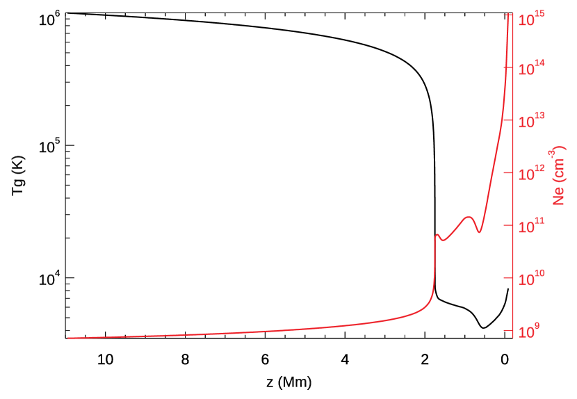
Figure 1: Initial atmospheric temperature (black) and electron density (red). The length coordinate z is measured along the loop with zero at $\tau_{\rm 500\,nm}$=1. The loop apex is at z=11 Mm.

Figure 2: Extra heating applied to sustain a VAL3C-like initial atmosphere. The constant value in the chromosphere, transition region, and corona is $1.9\times 10^{9}$ erg s^-1 g^-1.

5 Model grid

The F-CHROMA grid of models presented here have the same initial atmosphere (see Section 4); the parameters that vary are the beam parameters. We employed a triangular shape for the beam energy flux as a function of time with a linear increase in beam flux from zero at t=0 to a maximum at t=10 s and then a linear decrease to zero beam flux at t=20 s. The rationale for this profile is the typical rapid rise and decay of the impulsive time profiles of the higher energy hard X-ray bursts that map the energy input in the form of non-thermal electrons (e.g. de Jager & de Jonge, 1978; Dennis, 1985). There is evidence for shorter timescale variations (e.g. Aschwanden et al., 1995), but typically these have a smaller amplitude modulation, and the injection time profile does not include these. The simulations were continued with zero beam flux for an additional 30 s until t=50 s to capture the longer-timescale evolution of the atmosphere once direct beam heating stopped (e.g. the effects of conduction to the chromosphere from the hot coronal loop). The top and bottom boundary conditions were closed so the later time evolution might be influenced by reflection at the boundaries. We have varied the spectral index $\delta$, the total energy, and the low-energy cutoff $E_{c}$; readers can refer to table 5 for the values. We note that we label the models with the total energy; a total energy of $3\times 10^{10}$ erg cm^-2 corresponds to a maximum energy flux of $3\times 10^{9}$ erg cm^-2 s^-1. The output file naming convention is best illustrated with an example:
radyn_out.val3c_d3_1.0e12_t20s_25kev_fp
is the output file with a VAL3C-like starting atmosphere, a spectral index $\delta$=3, a total energy of $1\times 10^{12}$ erg cm^-2, a triangular time variation of the beam flux with a total duration of 20 s, a low-energy cutoff of 25 keV, and a Fokker-Planck description of the beam.

Table 5: Parameter values for the grid.

Parameter	values
$\delta$	3,4,5,6,7,8
$E_{\rm tot}$	$3\times 10^{10},1\times 10^{11},3\times 10^{11},1\times 10^{12}$ erg cm-2
$E_{c}$	10, 15, 20, 25 keV

6 Properties of the grid models

Different beam parameters lead to differences in the penetration depth of the beam. A lower value of the spectral index $\delta$ leads to a higher proportion of high-energy electrons and thus more heating low down in the atmosphere (Fig. 3). A higher value of the low-energy cutoff, $E_{c}$, also leads to more high-energy electrons and heating lower down (Fig. 4); readers can also refer to the discussion in Allred et al. (2015). The figures show heating per volume. Since the density decreases with height because of the hydrostatic stratification, heating per particle decreases deeper in the chromosphere.

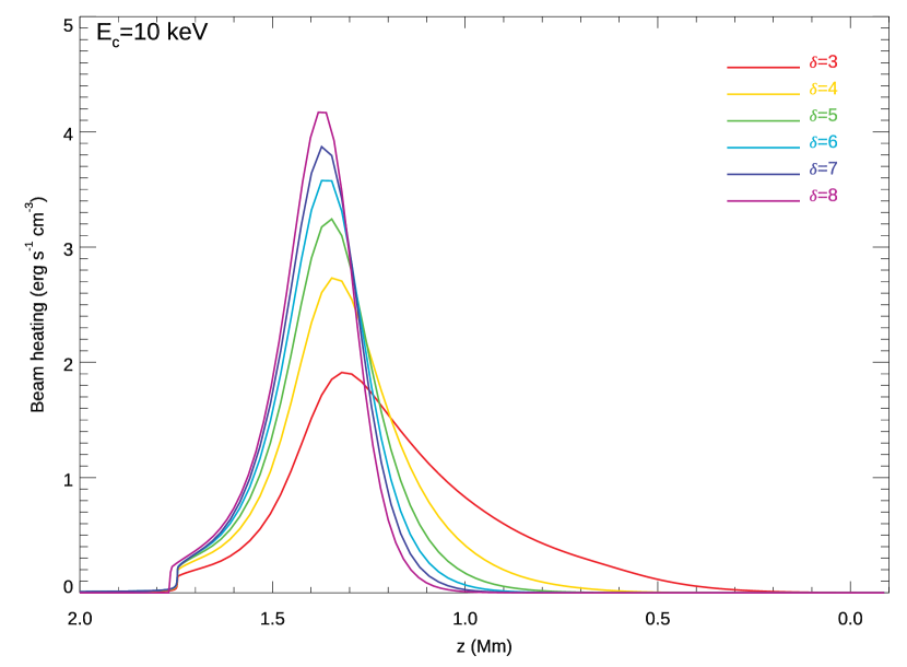
Figure 3: Beam heating at t=0.1s as function of height and spectral index for models with a low-energy cutoff of 10 keV. The total beam heating at this time is $1\times 10^{8}$ erg cm^-2 s^-1.

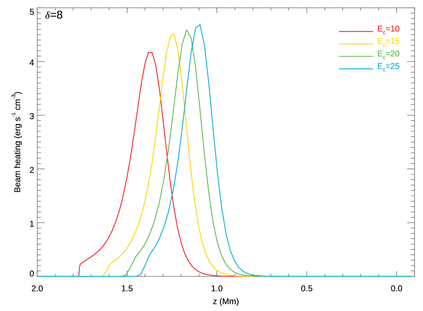
Figure 4: Beam heating at t=0.1s as function of height and low-energy cutoff for models with a spectral index of 8. The total beam heating at this time is $1\times 10^{8}$ erg cm^-2 s^-1.

With time, the heating profile as a function of height changes. The heating causes chromospheric evaporation and ionisation, and the density increases above where the beam heating takes place. This causes more of the beam energy to be deposited at larger heights. The variation of the heating profile with the beam parameters causes differences in the hydrodynamic response of the atmosphere. Figure 5 shows the temperature as a function of position, z, and time for the four different values of the low-energy cutoff and a total energy of $10^{11}$ erg cm^-2 and a spectral index of 3. For the lowest value of the low energy cutoff (upper left panel), the large proportion of low-energy electrons are collisionally stopped in the corona, leading to substantial heating there, expansion of the coronal plasma, and a transition region that moves downwards. A similar phenomenon was observed in simulations by Liu et al. (2009) and is consistent with hot downflows at flare footpoints such as those that were observed by Milligan & Dennis (2009). With an increasing low-energy cutoff, the heating moves deeper, and we see less coronal heating, more chromospheric heating, and a transition region moving upwards. This evolution is also seen in the bulk velocities (Fig.6) where the smallest low-energy cutoff leads to large velocities in the corona (outflow of several hundred km s^-1) and also large chromospheric condensation velocities, while stopping the beam deeper down at larger densities leads to smaller velocities. The chromospheric condensation leads to an increased density moving downwards and the chromospheric evaporation leads to increased densities higher up (Fig: 7).

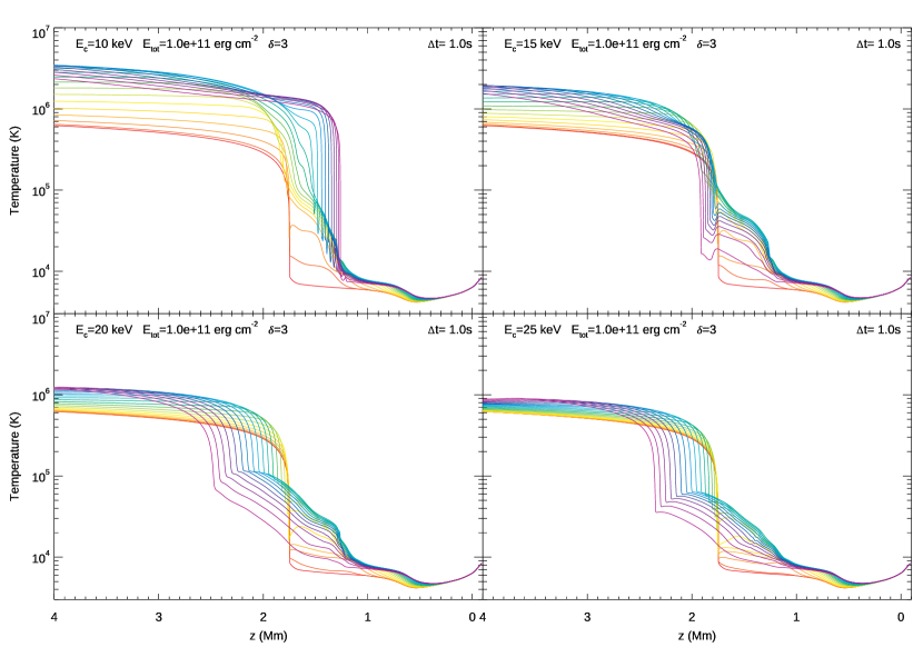
Figure 5: Temperature as function of loop position, z, and time for the four different values of the low-energy cutoff, a total energy of $10^{11}$ erg cm^-2, and a spectral index of 3. The initial temperature structure is shown in red, with subsequent timesteps, separated by 1.0s, shown with rainbow colours from red to violet. The last timestep shown is at t=20s, when the beam was switched off.

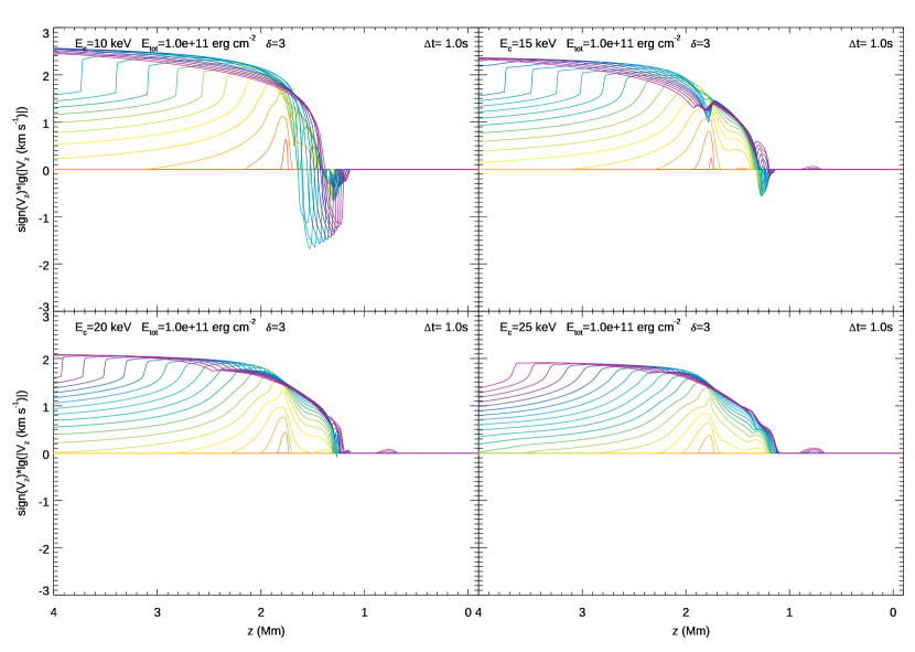
Figure 6: Bulk velocity as function of loop position, z, and time for the four different values of the low-energy cutoff, a total energy of $10^{11}$ erg cm^-2, and a spectral index of 3. The logarithm of the absolute value of the bulk velocity is shown, multiplied by the sign of the velocity. A value of one thus corresponds to an outflow of 10 km s^-1, minus one to an inflow of 10 km s^-1. Absolute values of the bulk velocity below 1 km s^-1 are shown as zero. The initial velocity of zero is shown in red, with subsequent timesteps, separated by 1.0s, shown with rainbow colours from red to violet. The last timestep shown is at t=20s, when the beam was switched off.

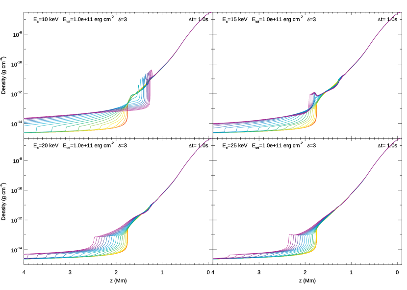
Figure 7: Mass density as function of loop position, z, and time for the four different values of the low-energy cutoff, a total energy of $10^{11}$ erg cm^-2, and a spectral index of 3. The initial density structure is shown in red, with subsequent timesteps, separated by 1.0s, shown with rainbow colours from red to violet. The last timestep shown is at t=20s, when the beam was switched off.

If the beam energy is deposited in the uppermost part of the chromosphere, we may get a temperature runaway leading to explosive evaporation. This happens because the optically thin loss curve has a maximum around 10${}^{5}\,$K such that when the temperature reaches this value, increased heating leads to decreased radiative losses. We see this in the temperature evolution with time for different values of the spectral index, $\delta$, in Fig.8. The temperature runaway in the upper chromosphere may leave a chromospheric bubble between the runaway part and the original transition region; readers can refer to Reid et al. (2020) for more details.

Obviously, the atmospheric evolution strongly depends on the total energy input. One example of the interplay between coronal and chromospheric heating for the span of total energy is shown in Fig. 9.

These examples are only meant to give an idea of the rich and varied atmospheric behaviour as a function of the beam parameters that can be explored with these models — an extensive analysis is beyond the scope of this paper. A more detailed analysis of some aspects can be found in the RADYN F-CHROMA grid papers referred to in Section 1.

7 Grid archive

All models are available from a searchable wiki-based archive page. The full RADYN source code is also available. Unpacking the tar file creates a directory radyn_fchroma with subdirectories. The file radyn_fchroma/doc/radyn_manual.pdf contains the manual and radyn_fchroma/doc/analysis_tools.pdf contains the instructions on how to read the CDF files and also a list of variables. It is also possible to download just the analysis software and its documentation.

Appendix A Additional figures

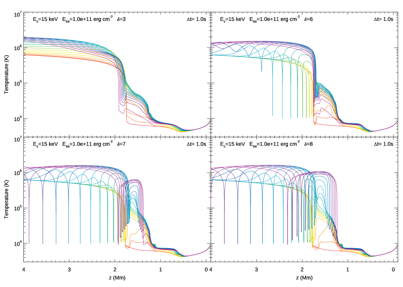
Figure 8: Temperature as function of loop position, z, and time for four different values of the spectral index, $\delta$, a lower-energy cutoff of 15 keV, and a total energy of $10^{11}$ erg cm^-2. The initial temperature structure is shown in red, with subsequent timesteps, separated by 1.0s, shown with rainbow colours from red to violet. The last timestep shown is at t=20s, when the beam was switched off.

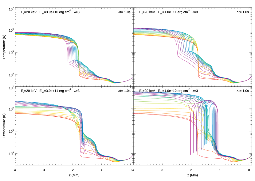
Figure 9: Temperature as function of loop position, z, and time for the four different values of the total energy, a lower-energy cutoff of 20 keV, and a spectral index of 3. The initial temperature structure is shown in red, with subsequent timesteps, separated by 1.0s, shown with rainbow colours from red to violet. The last timestep shown is at t=20s, when the beam was switched off.