Efficient Quantum Algorithms for Quantum Optimal Control

Abstract

In this paper, we present efficient quantum algorithms that are exponentially faster than classical algorithms for solving the quantum optimal control problem. This problem involves finding the control variable that maximizes a physical quantity at time $T$, where the system is governed by a time-dependent Schrödinger equation. This type of control problem also has an intricate relation with machine learning. Our algorithms are based on a time-dependent Hamiltonian simulation method and a fast gradient-estimation algorithm. We also provide a comprehensive error analysis to quantify the total error from various steps, such as the finite-dimensional representation of the control function, the discretization of the Schrödinger equation, the numerical quadrature, and optimization. Our quantum algorithms require fault-tolerant quantum computers.

1 Introduction

Optimal control is an important application of machine learning and optimization. Meanwhile, it has been demonstrated in recent works that important insights on deep learning can be obtained by interpreting the process of training a deep neural network as a discretization of an optimal control problem [18, 26]. In recent decades, following the emergence of quantum computers, the optimal control of quantum systems has attracted considerable attention. This is because quantum properties are largely responsible for many of the recent developments in material science and chemical engineering, and such properties are best utilized with external controls. [22, 16, 42]. Quantum optimal control (QOC) algorithms [5, 46], which uses first principle-based computer simulations to identify the desired control variable, has been an important route toward this direction. QOC problems have also emerged in recent quantum computing and quantum information technology. For example, QOC has recently been shown to have remarkable connections and applications to machine learning techniques using quantum circuits, including variational quantum algorithms (VQA) [11, 48], quantum neural networks [35], and quantum approximate optimization algorithm (QAOA) [20, 8, 36]. QOC is treated as a particular machine learning application in [2]. One specific application of QOC to quantum machine learning is the diagnostics of quantum barren plateau [34]. In addition, solving the optimal control problems for quantum systems is a critical step for implementing quantum computers.

The problem of controlling a quantum system can be formulated based on the time-dependent Schrödinger equation (TDSE),

$$i\partial_{t}\ket{\psi}=\big{(}{H}_{0}-u(t)\mu\big{)}\ket{\psi},\ket{\psi(0)}=\ket{\psi_{0}},$$ (1)

with an external control variable $u(t)$ that enters the Hamiltonian through an operator $\mu.$ One example comes from electron transport, where $H_{0}=-\frac{\nabla^{2}}{2}+V(x)$ and $\mu$ is the dipole operator. To keep our discussions focused on the quantum algorithms, we consider the case with a single control. The treatment of multiple control variables and non-unitary dynamics will be presented in separate works. We assume the copies of the initial state $\ket{\psi_{0}}$ are given for free, i.e., we have access to the unitary $U_{\psi_{0}}$ that prepares $\ket{\psi_{0}}$ as $U_{\psi_{0}}\ket{0}=\ket{\psi_{0}}$.

The goal of QOC with time duration $T$ is to determine a control variable $u(t)$ for $t\in[0,T]$, such that a physical quantity, represented by a Hermitian operator $O,$ is maximized in that

$$\max_{u(t)}J(u),\quad J(u)\coloneqq\langle\psi(T)|O|\psi(T)\rangle-\alpha\int_{0}^{T}|u(t)|^{2}\differential t.$$ (2)

Here $\alpha>0$ can be regarded as a regularization parameter imposing a soft constraint on the magnitude of the control variable $u(t)$. In the context of optimization, the function $J(u)$ is the objective (fitness) function. Aside from the generalization to multiple control variables, another straightforward extension is to control signals with explicit parametric forms, e.g., a trigonometric expression $u(t)=\sum_{j}E_{j}\cos(\omega_{j}t)e^{-(t-t_{j})^{2}/\sigma_{j}}$ modulated by a Gaussian envelope, which can be written in an abstract form as $u(t)=F(t,\bm{\theta})$ with $\theta$ embodying all the parameters. Then the objective function in Eq. 2 can be optimized over $\bm{\theta}$ and the gradient can be trivially obtained using chain rule: $\partial J/\partial\bm{\theta}=(\partial J/\partial u)\,\partial F/\partial\bm{\theta}.$ By restricting the control variable $u(t)$ to square-integrable functions, the objective function is clearly upper bounded. In addition, it is lower semicontinuous, which then implies that a maximum exists [12]. But in practice, the function is often nonconvex and possesses multiple maxima.

In addition to the wide range of applications of QOC, there is a host of mathematical analysis and computational techniques based on classical algorithms [6, 46, 19, 25, 12, 27, 14, 15, 1]. The present paper, however, will be concerned with computer simulations using quantum algorithms, where the $n$-qubit Hamiltonian operator $H$ (resp. $\mu$) is represented as a $2^{n}$-dimensional matrix $H\in\mathbb{C}^{2^{n}\times 2^{n}}$ (resp. $\mu\in\mathbb{C}^{2^{n}\times 2^{n}}$). In this paper, we assume the Hamiltonians $H$, $\mu$, and the observable $O$ are $d$-sparse: there are at most $d$ nonzero entries in each row/column. In other words, these matrices are efficiently row/column computable. To access these matrices, we assume we have access to a procedure $\mathcal{P}_{A}$ for a matrix $A$ that can perform the following mapping:

$$\ket{i}\ket{0}\mapsto\ket{i}\ket{r_{i,k}},$$ (3)

where $r_{i,k}$ is the $k$-th nonzero entry of the $i$-th row of $A$. In addition, $\mathcal{P}_{A}$ can also perform the following mapping:

$$\ket{i}\ket{j}\ket{0}\mapsto\ket{i}\ket{j}\ket{A(i,j)}.$$ (4)

Note that it is easy to adapt our algorithms to other more general input models, such as the block-encoding [38, 9].

With quantum access to these matrices, we aim to determine $u(t)$ for all $t$ such that the objective function defined in Eq. 2 is maximized. However, due to the nonconvex landscape of the objective function, finding the global maximum is not realistic. Instead, we consider the notion of $\epsilon$-first- or second-order convergence conditions (see Eqs. 12 and 13) for the objective function. More specifically, we aim to solve the following problem.

Problem 1.1.

Consider the $n$-qubit QOC in Eq. 2 for time duration $T$. Assume $\norm{H_{0}},\norm{O},\norm{\mu}\leq 1$, and $\alpha\geq 2/T$. Let $N$ be the number of time intervals and define $\delta\coloneqq T/N$. Suppose $H_{0}$, $\mu$ and the observable $O$ are $d$-sparse, and suppose we are given access to $U_{\psi_{0}}$ for preparing $\ket{\psi_{0}}$. Given the sparse access $\mathcal{P}_{H_{0}}$ to $H_{0}$, $\mathcal{P}_{\mu}$ to $\mu$, and $\mathcal{P}_{O}$ to $O$, determine $\tilde{u}(t_{j})$ ($t_{j}=j\delta$) for all $j\in[N]$ such that $\big{|}\tilde{u}(t_{j})-u(t_{j})\big{|}\leq\epsilon$, where $u(t)$ is an $\epsilon$-first-order stationary point of $J(u)$ satisfying Eq. 12 or an $\epsilon$-second-order stationary point satisfying Eq. 13.

The main challenge in solving 1.1 is due to the repeated solution of TDSE in Eq. 1, which becomes unfavorable for classical computers because the dimension grows exponentially. In addition, many optimization algorithms require the computation of the derivatives of the objective function with respect to the control variable $u(t).$ A direct calculation of such derivatives of $J$ in Eq. 2 also requires visiting the TDSE. The most well-known classical method for optimizing Eq. 2 is due to Zhu and Rabitz [50]. The idea is to regard the TDSE in Eq. 1 as a constraint, which is incorporated into the objective function using a Lagrange multiplier. For this optimization problem, algorithms can be constructed by enforcing the first-order condition. Zhu and Rabitz [50] established the monotone convergence property of this algorithm. This approach is later extended to further improve the convergence properties [41, 19, 12] including formulations based on the Liouville von Neumann equation.

Nevertheless, the complexity associated with one iteration of these classical algorithms has the scaling of $\mathcal{O}\big{(}\mathrm{poly}(2^{n})T\big{)}$, where $n$ is the number of system qubits and we did not include $\epsilon$ in the complexity. The exponential dependence on $n$ comes from the fact that at each time step, the wave functions have to be computed from previous time steps using an approximation of the unitary operator. Depending on the specific methods, this may involve matrix multiplications or solutions of a linear system of equations [7]. The exponential scaling significantly limits the scope of the application, since $2^{n}$ is usually proportional to the domain size and the number of electrons.

Main Contributions. In this paper, we present efficient quantum algorithms for solving the quantum optimal control problem defined in Eq. 2 that scale polynomially in $n$ — our quantum algorithms have exponential speedups compared with best known classical algorithms. One key contribution is a complexity analysis that takes into account various error contributions, including (i) the finite-dimensional approximation of $u(t)$, (ii) the discretization of the objective function in Eq. 2, (iii) the approximation of the wave function, and (iv) the optimization error. Such comprehensive overall estimates are extremely valuable to assess the resources needed for a specific QOC problem. We start with the Hamiltonian simulation method for time-dependent problems [4] to access the objective function, thus enabling a quantum gradient estimation [23] approach, so that a gradient-based optimization method can be applied. Although our approach is formulated for the TDSE, it can be readily generalized to other control problems where the dynamics is not Hamiltonian, e.g., ODEs implemented with quantum spectral method [10].

The following theorem summarizes our main result, where the $\widetilde{\mathcal{O}}$ notation has omitted logarithmic factors.

Theorem 1.2 (Summarizing Theorem 3.9 and Theorem 4.1).

Assume that $u(t)\in\mathrm{C}^{2}([0,T]).$ There exists a quantum algorithm that, with probability at least $2/3$, solves 1.1 using $\mathcal{\widetilde{O}}\left(\frac{dLT^{2}}{\epsilon^{3}}\right)$ queries to $\mathcal{P}_{H_{0}}$ and $\mathcal{P}_{\mu}$, and $\widetilde{\mathcal{O}}\left(\frac{dnLT^{2}}{\epsilon^{3}}+\frac{LT^{3/2}}{\epsilon^{5/2}}\right)$ additional 1- and 2-qubit gates.

Further, when the control variable $u(t)$ is smooth, the gate complexity becomes $\widetilde{\mathcal{O}}\left(\frac{dnLT^{2}}{\epsilon^{3}}+\frac{LT}{\epsilon^{2}}\right)$. The Lipschitz constant $L$ can be bounded by Eq. 15

Although the smooth control variables does not improve the gate complexity asymptotically, it can reduce the number of gates in practical implementations. We also use Table 1 for a clear comparison of different smoothness assumptions on the control variable $u(t)$.

Smoothness	Queries	Additional gates
Without smoothness	$\mathcal{\widetilde{O}}\left(\frac{{dLT^{2}}}{\epsilon^{3}}\right)$	$\widetilde{\mathcal{O}}\left(\frac{dnLT^{2}}{\epsilon^{3}}+\frac{LT^{3/2}}{\epsilon^{5/2}}\right)$
Smooth control	$\mathcal{\widetilde{O}}(\frac{dL{T}^{2}}{\epsilon^{3}})$	$\widetilde{\mathcal{O}}\left(\frac{dnLT^{2}}{\epsilon^{3}}+\frac{LT}{\epsilon^{2}}\right)$

Table 1: The query and gate complexities for solving 1.1.

It is important to note that our algorithms require fault-tolerant quantum computers, and hence they are not suitable for near-term quantum devices.

Related work. To the authors’ knowledge, the first attempt to solve the quantum control problem using quantum algorithms has been proposed by [37]. This approach requires a classical device to update the control variable $u(t)$ using a gradient-based method. More recently, Brif et al. [5] considered a specific application, where a molecular wave function is evolved under a laser pulse. The algorithm is also hybrid in nature, utilizing a classical device to update the control variable. The approach outputs the objective function, rather than the gradient, for the Nelder-Mead optimization method. None of the above-mentioned works uses the full power of quantum computation, including the state-of-the-art quantum algorithms for Hamiltonian simulation algorithms and gradient estimation. More importantly, precise query complexity that takes into account all levels of approximations is not provided, making it difficult to assess the applicability of the algorithms to specific quantum control problems in practice.

The QOC problems show great similarity with variational quantum algorithms (VQA) in general [8], except that in most VQAs, the unitary operations are associated with parameterized gates, rather than time-dependent Hamiltonians in QOC, where the smoothness of the control function also plays a role in the error. Several other algorithms have recently been proposed to help with the computation of the gradient in VQA [13, 47, 33].

Very recently, Leng, Peng, Qiao, Lin, and Wu [36] proposed a differentiable programming framework for quantum computers to evaluate gradients of time-evolved states. One of their application is QOC. In their model, the control function $u(t)$ is fixed while leaving freedoms to the parameters of $u$ to be tuned. In contrast, we work on a more general control model and deal with the control function in real time directly. In addition, our work focuses on quantum algorithms on fault-tolerant quantum computers, and we use state-of-the-art techniques to improve the complexity.

Notation. We provide a brief introduction to quantum computation in Section 2.1. Here, we summarize the notations used in this paper. First of all, we should distinguish quantum states from a vector in the context of classical computation, although a quantum state is mathematically represented as a vector. In the context of quantum dynamics, we use the Dirac notation $\ket*{\cdot}$ to represent quantum states. For vectors in the context of classical computation, e.g., the gradient vector and the control variable at multiple time steps, we use the bold font, e.g., $\bm{u}$. For a positive integer $k$, we use $[k]$ to denote the set $\{1,\ldots,k\}$. For a vector $\bm{u}$, we use the subscript with a normal font to denote its entries, i.e., $u_{1},\ldots,u_{d}$ are the entries of $\bm{u}$. For a vector $\bm{u}$, we use $\norm{\bm{u}}$ to denote its Euclidean norm, i.e., $\norm{\bm{u}}=\sqrt{\sum_{j=1}^{d}|u_{j}|^{2}}$. We use $\norm{\bm{u}}_{\infty}$ to denote its maximum norm, i.e., $\norm{\bm{u}}_{\infty}=\max_{j}|u_{j}|$.

In addition, we denote by $\mathrm{C}^{2}[0,T]$ the class of twice continuously differential functions defined in $[0,T]$. For a function $f$, we use $\norm{f}_{2}$, or $\norm{f(t)}_{2}$ to denote its $L_{2}$ norm. Namely, $\norm{f(t)}_{2}=\norm{f}_{2}=\int_{0}^{T}f(t)^{2}\,\differential t$.

2 Preliminaries

To solve 1.1, we need to deal with several levels of approximations, including a finite-dimensional representation of the function $u(t)$, the time discretization of the TDSE in Eq. 1, the approximation of the gradient of $\bra{\psi(T)}O\ket{\psi(T)}$, and the optimization error. In this section, we first give a simplistic yet sufficient introduction to quantum computation. Then we analyze the error caused by the discretization of $u(t)$, the discretization of the TDSE, and optimization in subsequent subsections.

2.1 A brief introduction to quantum computation

The most daunting obstacle for learning quantum computing is probably its notations. Once one is getting familiar with the Dirac notation, quantum computing can be understood as matrix-vector multiplications. For an $n$-qubit state, we use a $2^{n}$-dimensional complex (column) vector with unit Euclidean norm to mathematically describe it, and this vector is denoted, in the Dirac notation, by $\ket{\psi}$. We use $\bra{\psi}$ to denote the conjugate transpose of $\ket{\psi}$, and then the inner product between two states can be conveniently written as $\innerproduct{\psi}{\phi}$. When the symbol in the Dirac notation is a natural number, i.e., $\ket{0},\ldots,\ket{2^{n}-1}$, we use such states to specifically denote the set of the standard basis of a $2^{n}$-dimensional vector space, same as the basis vectors $\bm{e}_{0},\ldots,\bm{e}_{2^{n}-1}$ that we usually see in linear algebra textbooks. With respect to the standard basis, let $\alpha_{0},\ldots,\alpha_{2^{n}-1}$ be the entries of $\ket{\psi}$, i.e., $\ket{\psi}=\bigl{[}\alpha_{0},\ldots,\alpha_{2^{n}-1}\bigr{]}^{T}$. It can be conveniently written as a superposition, $\ket{\psi}=\alpha_{0}\ket{0}+\cdots+\alpha_{2^{n}-1}\ket{2^{n}-1}$. When $\ket{\psi}$ is measured, with probability $|\alpha_{j}|^{2}$, it will collapse to $\ket{j}$. Note that a measurement is an irreversible process: a state cannot be restored once it collapses to some basis state.

The building blocks of quantum algorithms are 1- and 2-qubit gates: they are modeled as $2\times 2$ (1-qubit), or $4\times 4$ (2-qubit) unitary matrices. A network of quantum gates form a quantum circuit, which, acting on $n$ qubits, is mathematically represented as a $2^{n}\times 2^{n}$ unitary matrix. In essence, a quantum algorithm starts from an $n$-qubit initial state $\ket{0}$ that is easy to prepare, and applies a quantum circuit, represented by $U$, yielding the state $\ket{\psi}=U\ket{0}$. Then a measurement is performed on $\ket{\psi}$ to obtain the desired outcomes. Readers may refer to [44] for a thorough introduction to quantum computation.

2.2 Approximation Error of the Objective Function

We first represent the control variable $u(t)$ at finitely many time steps with the length of a time interval denoted by $\delta$: Let $t_{j}=j\delta$ be discrete time steps, and $N=T/dt$ be the number of time steps. Then we represent $u(t)$ via piece-wise linear interpolation, denoted by $u_{I}(t)$, given by,

$$u_{I}(t)=\sum_{j=0}^{N}u_{j}b_{j}(t),$$ (5)

with $b_{j}(t)$ being the nodal basis functions (i.e., the hat functions) centered at time steps $t_{j}$. The interpolating function can also be integrated directly, which leads to a quadrature approximation for the integral in Eq. 2. The error from these approximations follows the standard error bound, e.g., see [32].

Theorem 2.1 (Perturbation under $\mathrm{C}^{2}$ assumption.).

Assume that $u(t)\in\mathrm{C}^{2}([0,T]),$ i.e., it is twice continuously differentiable, then the error from the piecewise-linear interpolation is bounded as follows,

$$\|u(t)-u_{I}(t)\|_{2}\leq C\|u^{\prime\prime}(t)\|_{2}\delta^{2}.$$ (6)

In addition, the integral of $u(t)^{2}$ can be approximated by a composite trapezoid rule, with weights denoted by $w_{j}$,

$$\int_{0}^{T}u(t)^{2}\,\differential t=\delta\sum_{j=0}^{N}w_{j}u(t_{j})^{2}+\mathcal{O}\left(T\delta^{2}\right).$$ (7)

The quadrature formula ($w_{0}=w_{N}=1/2$ and $w_{1}=w_{2}=\cdots=w_{N-1}=1$) can be derived from the linear interpolation of $u(t)$ in each time interval by integrating the nodal functions directly. In addition, the error carries a prefactor that is proportional to the second-order derivatives of the integrand, which is bounded due to the assumption that $u(t)\in\mathrm{C}^{2}([0,T]).$

With this representation of the control function, the problem is reduced to a finite-dimensional problem. We will use $\bm{u}$ to represent the nodal values of the interpolation: $\bm{u}=\big{\{}u_{j}\big{\}}_{j=1}^{N}$, with $u_{j}$ being the nodal value of $u(t)$ at $t_{j}.$ We will then write the corresponding objective function as $\widetilde{J}(\bm{u}),$ a function with $N$ variables. Namely,

$$\widetilde{J}(\bm{u})=\bra{\psi_{N}}O\ket{\psi_{N}}-\alpha\delta\sum_{j=0}^{N}w_{j}u_{j}^{2}.$$ (8)

Here we have also included the approximation of $\ket{\psi(T)}$, denoted by $\ket{\psi_{N}}$.

Corollary 2.2.

Assume that the wave function is approximated by $\ket{\psi_{N}}$, with an error comparable to the quadrature error in Eq. 7, i.e.,

$$\norm{\ket{\psi_{N}}-\ket{\psi(T)}}=\mathcal{O}(T\delta^{2}).$$ (9)

Further assume that the maximum of $J[u]$ is achieved at some $u^{*}(t)\in\mathrm{C}^{2}([0,T])$, and the maximum is not degenerate. Then for sufficiently small $\epsilon,$ by choosing,

$$N=\mathcal{O}\left({\frac{T^{3/2}}{\epsilon^{1/2}}}\right),$$ (10)

the approximate objective function $\widetilde{J}(\bm{u})$ has a maximum $\bm{u}^{*},$ for which the corresponding interpolant satisfies,

$$\norm{u(t)-u_{I}(t)}_{2}\leq\epsilon.$$

Proof.

This can be proved by using the continuous dependence of the wave function $\ket{\psi(t)}$ on the control variable $u(t)$, e.g., see Proposition 4 of [12]. ∎

2.3 Optimization method

A gradient-base algorithm updates the control variables using the gradient [43] to generate an approximating sequence $\{\bm{u}^{(k)}\}_{k\geq 0}$,

$$\bm{u}^{(k+1)}=\bm{u}^{(k)}+\eta\big{(}\nabla J(\bm{u}^{(k)})+\bm{\zeta}_{k}\big{)}.$$ (11)

Notice that the QOC in Eq. 2 is customarily formulated as a maximization problem. Therefore, the algorithm updates the control variables along the gradient ascent direction. In addition, we considered the perturbed gradient method [29], which introduced a Gaussian noise $\bm{\zeta}_{k}$ with mean zero and $\mathbb{E}[\bm{\zeta}_{k}^{2}]=r^{2}$ for some $r>0$ to help the solution with fulfilling an approximation second-order condition.

The convergence to the global maximum of a gradient-based algorithm requires certain convexity assumptions on $J$, e.g., the star-convexity [49], which, however, may not be easy to verify in practice. Alternatively, one can seek approximate optimality conditions. Jin et al. [29] introduced $\epsilon$-first and second order conditions,

$$\norm{\nabla J(\bm{u})} <\epsilon,\;\text{and}$$ (12)

$$\nabla^{2}J(\bm{u}) \leq\sqrt{\rho\epsilon}I.$$ (13)

Here $\rho$ is the Lipschitz constant of the Hessian. The following result, adapted from Theorem 4.1 of [29] (with $\sigma=\mathcal{O}(\epsilon^{2})$ ) summarizes the complexity associated with optimization.

Theorem 2.3 (Adapted from Theorem 4.1 in [29]).

Assume that the gradient $\nabla J$ is $L-$Lipschitz and it can be estimated with an unbiased estimation of variance $\sigma^{2}=\mathcal{O}{(\epsilon^{2})}$ and that the learning rate is $\eta<\Theta\left(\frac{1}{L}\right)$. With probability at least $1-\delta$, the optimization method defined in Eq. 11 will visit an approximate stationary point that fulfills the first order conditions in Eq. 12, at least once within the following number of iterations,

$$k=\widetilde{\mathcal{O}}\left(\log\frac{1}{\delta}L\frac{J(\bm{u}^{*})-J(\bm{u}^{(0)})}{\epsilon^{2}}\right).$$ (14)

For the objective function in Eq. 8, the Lipschitz constant can be estimated using the derivative bounds from Lemma 3.5,

$$L\leq T\delta\norm{\mu}^{2}+2\alpha\delta.$$ (15)

Since we do not assume an upper bound on $\alpha$, we will treat $L$ as a separate constant.

3 Quantum algorithm and complexity analysis

In order to access the objective function in Eq. 2, a time discretization is needed to approximate the integral and the wave function $\psi(T)$ by numerical integrators, as alluded to in the previous section. To begin with, we write $\widetilde{J}$ as two terms: $\widetilde{J}(\bm{u})=\widetilde{J}_{1}(\bm{u})+\widetilde{J}_{2}(\bm{u})$, where

$$\widetilde{J}_{1}(\bm{u}) \coloneqq\bra{\psi_{N}}O\ket{\psi_{N}}\quad\text{ and}$$ (16)

$$\widetilde{J}_{2}(\bm{u}) \coloneqq\alpha\delta\sum_{j=1}^{N}w_{j}u(t_{j})^{2}.$$ (17)

Note the $\widetilde{J}_{2}$ is easy to compute on a classical computer. Thus we only focus on $\widetilde{J}_{1}$, and use a quantum algorithm to speed up its calculation.

3.1 Obtaining the final state

To have quantum access to $\widetilde{J}_{1}$, we need to efficiently prepare of $\ket{\psi_{N}}$ via a time-marching procedure, i.e.,

$$\ket{\psi_{N}}=V(t_{N},t_{N-1})V(t_{N-1},t_{N-2})\cdots V(t_{1},t_{0})\ket{\psi_{0}}.$$ (18)

Note that $t_{N}=T$. At each step, the dynamics is evolved via an operator $V(t_{j},t_{j-1})$. For instance, in the Dyson series approach [39, 31], the operator $V$ can be constructed as follows,

$$\begin{aligned} V(&t_{j+1},t_{j})=\\ &\sum_{k=0}^{K}\frac{(-i\delta)^{k}}{M^{k}k!}\sum_{j_{1},j_{2},\cdots,j_{k}=0}^{M-1}\mathcal{T}H(s_{j_{k}})\cdots H(s_{j_{1}}).\end{aligned}$$ (19)

Here the symbol $\mathcal{T}$ indicates that only those points where $s_{j_{1}}\leq s_{j_{2}}\leq\cdots\leq s_{j_{k}}$ are collected. The points are selected to approximate the integrals in the Dyson series expansion [3]. The complexity estimate was presented in Theorem 9 of [39]. We use a more efficient simulation algorithm by Berry, Childs, Su, Wang, and Wiebe [4] where the dependence on $T\max_{t}\norm{H(t)}_{\max}$ has later been relaxed to an averaged $L_{1}$ norm in time.

Lemma 3.1 ([4]).

Assume that $n$-bit Hamiltonian $H(t)$ is $d$-sparse for all $t\in[0,T]$. The TDSE in Eq. 1 can be simulation until time $T$ within error $\epsilon$ and failure probability $\mathcal{O}(\epsilon)$ using

$$\mathcal{O}\left(d\int_{0}^{T}\,\differential\tau\norm{H(\tau)}_{\max}\frac{\log(dH_{\mathrm{max}}T/\epsilon)}{\log\log(dH_{\mathrm{max}}T/\epsilon)}\right),$$ (20)

queries to the oracle of $H(t)$ and $\widetilde{\mathcal{O}}(dn\int_{0}^{T}\,\differential\tau\norm{H(\tau)}_{\max})$ additional 1- and 2-qubit gates.

Once $\ket{\psi_{N}}$ from Eq. 18 is prepared by Lemma 3.1, we can use it to estimate the gradient of $\widetilde{J}$ defined in Eq. 8. We take advantage of quantum gradient estimation algorithms to estimate $\nabla\widetilde{J}$. These algorithms require certain quantum access to the function. In particular, we define the two commonly used oracles, namely, the probability oracle and the phase oracle as follows.

Definition 3.2 (Probability oracle).

Consider a function $f:\mathbb{R}^{d}\rightarrow[0,1]$. The probability oracle for $f$, denoted by $U_{f}$, is a unitary defined as

$$U_{f}\ket{\bm{x}}\ket{\bm{0}}=$$ (21)

$$\ket{\bm{x}}\left(\sqrt{f(\bm{x})}\ket{1}\ket{\phi_{1}(\bm{x})}+\sqrt{1-f(\bm{x})}\ket{0}\ket{\phi_{0}(\bm{x})}\right),$$

where $\ket{\phi_{1}(\bm{x})}$ and $\ket{\phi_{0}(\bm{x})}$ are arbitrary states.

Definition 3.3 (Phase oracle).

Consider a function $f:\mathbb{R}^{d}\rightarrow\mathbb{R}$. The phase oracle for $f$, denoted by $O_{f}$, is a unitary defined as

$$O_{f}\ket{\bm{x}}\ket{\bm{0}}=e^{if(\bm{x})}\ket{\bm{x}}\ket{\bm{0}}.$$ (22)

The following result from Theorem 14 of [23] shows an efficient conversion from the probability oracle to the phase oracle.

Lemma 3.4.

Consider a function $f:\mathbb{R}^{d}\rightarrow[0,1]$. Let $U_{f}$ be the probability oracle for $f$. Then, for any $\epsilon\in(0,1/3)$, we can implement an $\epsilon$-approximate of the phase oracle $O_{f}$ for $f$, denoted by $\widetilde{O}_{f}$, such that $\norm{\widetilde{O}_{f}\ket{\psi}\ket{\bm{x}}-O_{f}\ket{\psi}\ket{\bm{x}}}\leq\epsilon$, for all state $\ket{\psi}$. This implementation uses $\mathcal{O}(\log(1/\epsilon))$ invocations to $U_{f}$ and $U_{f}^{{\dagger}}$, and $\mathcal{O}(\log\log(1/\epsilon))$ additional qubits.

We will show how to construct the required oracle for $\widetilde{J}_{1}$ given the circuit that prepares $\ket{\psi_{N}}$ in the proof of Theorem 3.9. Before that, let us focus on higher-order derivatives of $\widetilde{J}_{1}$, which are crucial in quantum algorithms for estimating the gradient of $\widetilde{J}_{1}$.

3.2 High-order derivatives of the objective function

In this subsection, we bound the magnitude of higher-order derivatives of $\widetilde{J}_{1}$. In particular, we show the following lemma. The proof can be found in Appendix A.

Lemma 3.5.

Let $\bm{\alpha}=(\alpha_{1},\ldots,\alpha_{k})\in[N+1]^{k}$ be an index sequence. The derivatives of the control function $\widetilde{J}_{1}$ with respect to the control variables satisfy:

$$\norm{\frac{\partial^{\bm{\alpha}}\widetilde{J}_{1}}{\partial u_{\alpha_{1}}u_{\alpha_{2}}\cdots u_{\alpha_{k}}}}\leq(k+1)!\left(\delta\|\mu\|\right)^{k}.$$ (23)

3.3 Quantum gradient estimation

In this subsection, we show how to efficiently estimate the gradient of $\widetilde{J}_{1}$. In the following, we state a quantum algorithm for estimating gradients due to Gilyén, Arunachalam, and Wiebe [23], which is an extension Jordan’s gradient estimation algorithm [30]. Note that there exists a nearly-optimal gradient estimation, i.e., Theorem 25 of [23]; however, this result does not directly apply to our setting since the derivatives, as characterized in Lemma 3.5, do not satisfy the bound $c^{k}k^{k/2}$. To give a more efficient estimation algorithm than just relying on the bound on the Hessian, we use the following result based on a higher-order finite difference method.

Lemma 3.6 (Rephrased from Theorem 23 of [23]).

Suppose the access to $f:[-1,1]^{N}\rightarrow\mathbb{R}$ is given via a phase oracle $O_{f}$. If $f$ is $(2m+1)$-times differentiable and for all $\bm{x}\in[-1,1]^{N}$ it holds that

$$|\partial_{\bm{r}}^{2m+1}f(\bm{x})|\leq B\quad\text{ for $\bm{r}=\bm{x}/\norm{\bm{x}}$},$$ (24)

then there exists a quantum algorithm that output an approximate gradient $\bm{g}$ such that $\norm{\bm{g}-\nabla f(\bm{0})}_{\infty}\leq\epsilon$ with probability at least $1-\rho$ using

$$\widetilde{\mathcal{O}}\left(\frac{N^{1/2}B^{1/(2m)}N^{1/(4m)}\log(N/\rho)}{\epsilon^{1+1/(2m)}}\right)$$ (25)

queries to $O_{f}$, and $\widetilde{\mathcal{O}}(N)$ additional 1- and 2-qubit gates.

Based on Lemma 3.6, we have the following result, where the proof is postponed in Appendix B.

Lemma 3.7.

Let $\widetilde{J}_{1}$ be defined as in Eq. 16. Suppose we are given access to the phase oracle $O_{\widetilde{J}_{1}}$ for $\widetilde{J}_{1}$. Then, there exists a quantum algorithm that outputs an approximate gradient $\bm{g}$ such that $\norm{\bm{g}-\nabla\widetilde{J}_{1}}\leq\epsilon$ with probability at least $1-\rho$ using $\widetilde{\mathcal{O}}\left(T\log(N/\rho)/\epsilon\right)$ queries to $O_{\widetilde{J}_{1}}$, and $\widetilde{\mathcal{O}}(N)$ additional 1- and 2-qubit gates.

3.4 Proof of the main theorem

We outline the combined algorithm in Algorithm 1. The bound on $k_{\max}$ follows from Eq. 14.

Given $T>0$ and $\epsilon>0$, set $N=\frac{T^{3/2}}{\epsilon^{1/2}}$, and $k_{\max}=\mathcal{O}(\frac{L}{\epsilon^{2}})$ where $L$ is bounded by Eq. 15; set $u(t)=0$ ;

for $k=1:k_{\mathrm{max}}$ do

       Use Lemmas 3.1 and 3.4 to construct the phase oracle for $\widetilde{J}_{1}(\bm{u})$;

       Use Lemma 3.7 to estimate $\bm{g}^{(k)}\approx\nabla J(\bm{u}^{(k)})$;

       Update control variable: $\bm{u}^{(k+1)}=\bm{u}^{(k)}+\eta\bm{g}^{(k)}+\eta\bm{\zeta}_{k}$;

      

end for

Algorithm 1 Quantum algorithm for solving QOC

Before proving the performance of Algorithm 1, we need to bound the $L_{1}$ norm $\int_{0}^{T}\differential\tau\norm{H(t)}_{\max}$, which depends on the $L_{1}$ norm of control function. Although in general, no explicit formula is available for $u(t)$, we can deduce some a priori bounds on $u(t)$.

Lemma 3.8.

Suppose that $\norm{O}\leq 1,$ and $\alpha>\frac{2}{T}$. Let $u^{(1)},\ldots,u^{(k)}$ be a sequence of control variables obtained from each iteration of Algorithm 1. Let $u^{(1)}(t)=0$ be the initial guess. Then for all $j\in[k]$, the $L_{1}$ norms of the control functions satisfy $\int_{0}^{T}\absolutevalue{u^{(1)}(t)}\differential t\leq T$.

Proof.

First of all, note that $J(u^{(1)})\geq-1$. For all $j=2,\ldots,k$, we have $J(u^{(j)})\geq J(u^{(1)})\geq-1$. Again using the fact that $\norm{O}\leq 1$, we find $\int_{0}^{T}|u^{(j)}(t)|^{2}\differential t\leq 2/\alpha\leq T.$ Using Cauchy–Schwarz inequality, we have,

$$\int_{0}^{T}\absolutevalue{u^{(j)}(t)}\differential t\leq\left[\int_{0}^{T}\absolutevalue{u^{(j)}(t)}^{2}\differential t\right]^{\frac{1}{2}}{T}^{\frac{1}{2}}\leq T.$$ (26)

∎

The inequality $J(u^{(j)})\geq J(u^{(1)})$ follows from a function ascent property in Eq. 32, which as we will illustrate in the proof of Theorem 3.9, occurs with high probability. Because $\norm{H_{0}},\norm{\mu}\leq 1$, Lemma 3.8 implies that

$$\int_{0}^{T}\,\differential\tau\norm{H(t)}_{\max}=\mathcal{O}(T).$$ (27)

Now, we are ready to state the main result of this section.

Theorem 3.9.

Assume that $u(t)\in\mathrm{C}^{2}([0,T])$. There exists a quantum algorithm that, with probability at least $2/3$, solves 1.1 by visiting a first-order stationary point satisfying Eq. 12 using $\mathcal{\widetilde{O}}\left(\frac{dLT^{2}}{\epsilon^{3}}\right)$ queries to $\mathcal{P}_{H_{0}}$ and $\mathcal{P}_{\mu}$, and $\widetilde{\mathcal{O}}\left(\frac{dnLT^{2}}{\epsilon^{3}}+\frac{LT^{3/2}}{\epsilon^{5/2}}\right)$ additional 1- and 2-qubit gates. The Lipschitz constant $L$ can be bounded by Eq. 15.

Proof.

Recall that by using Lemma 3.1, we can obtain $\ket{\psi_{N}}$ given $\ket{\psi_{0}}$. Now, we show how to construct the oracle to estimate the gradient of $\widetilde{J}$. We first construct the probability oracle $U_{\widetilde{J}_{1}}$ for $\widetilde{J}_{1}$ by a Hadamard test circuit. Note that this oracle is well-defined because we have assumed that $\norm{O}\leq 1$. In addition, we need access to a block-encoding $U_{O}$ of $O$, which is a unitary of the form

$$U_{O}=\begin{bmatrix}O&\cdot\\ \cdot&\cdot\end{bmatrix}.$$ (28)

Hence, $\bra{0}\bra{\psi_{N}}U_{O}\ket{0}\ket{\psi_{N}}=\bra{\psi_{N}}O\ket{\psi_{N}}$. Let c-$U_{O}$ denote the controlled $U_{O}$. The Hadamard test circuit $(H\otimes I)(\text{c-}U_{O})(H\otimes I)$ acting on $\ket{0}\ket{\psi_{N}}$ produces,

$$\sqrt{f(\bm{u})}\ket{1}\ket{\phi_{1}(\bm{u}}+\sqrt{1-f(\bm{u})}\ket{0}\ket{\phi_{0}(\bm{u}},$$ (29)

for $f(\bm{u})\coloneqq-\frac{1}{2}\bra{\psi_{N}}O\ket{\psi_{N}}+\frac{1}{2}$. Note that we actually constructed the probability oracle for $f(\bm{u})$ instead of $\bra{\psi_{N}}O\ket{\psi_{N}}$. However, this is fine because the gradient of the latter is the gradient of the former multiplied by a factor $-1/2$. In addition, we note that the block-encoding $U_{O}$ can be efficiently constructed using the sparse-access oracles for $O$ (see Lemma 48 of [24]). It is important to note that the implementation of the time-dependent Hamiltonian simulation by using Lemma 3.1 uses some control variable $\bm{u}$ as part of the input. Such Hamiltonian simulation circuits can be made coherent, i.e., it can be used when the register containing the control variable $\bm{u}$ is in superposition. In addition, we use $U_{\psi_{0}}$ to prepare the initial state $\ket{\psi_{0}}$ from $\ket{0}$ for Hamiltonian simulation. Due to the bound on the $L_{1}$ norm in Eq. 27, we can implement the probability oracle $U_{\widetilde{J}_{1}}$ as defined in Definition 3.2 using $\widetilde{\mathcal{O}}(dT)$ queries to $\mathcal{P}_{H_{0}}$ and $\mathcal{P}_{\mu}$. We highlight that the oracle for the time-dependent Hamiltonian can be efficiently implemented. The values of the control function away from the nodal points can be easily computed by linear interpolation. Thus, we store $\mathcal{O}(N)$ parameters in QRAM to construct the input oracle. The gate complexity of the addressing scheme for QRAM is $\widetilde{\mathcal{O}}(N)$, which is polynomial in $T$ and $\epsilon$ due to Eq. 10. The circuit depth of the addressing scheme is $\mathcal{O}(\log N)$. As a result, considering the gate- and time-complexities of implementing QRAM, the Hamiltonian simulation is still efficient. Further, in special cases of our control models where the form of $u(t)$ is known, while the parameters in $u(t)$ need to be determined, we do not need QRAM because $u(t)$ can be computed by an efficient subroutine.

Next, we use Lemma 3.4 to construct an $\epsilon$-approximate phase oracle $\widetilde{O}_{f}$ defined in Definition 3.3 using $\mathcal{O}(1)$ queries to $U_{\widetilde{J}_{1}}$ and hence $\widetilde{\mathcal{O}}(dT)$ queries to $\mathcal{P}_{H_{0}}$ and $\mathcal{P}_{\mu}$.

Using Lemma 3.7, we can obtain a vector $\bm{g}$ such that $\norm{\bm{g}-\nabla\widetilde{J}_{1}/2}\leq\epsilon$ with probability at least $1-\rho$ using $\widetilde{\mathcal{O}}(T\log(N/\rho)/\epsilon)$ queries to $O_{\widetilde{J}_{1}}$. Hence, the number of queries to $\mathcal{P}_{H_{0}}$ and $\mathcal{P}_{\mu}$ is

$$\widetilde{\mathcal{O}}\left(\frac{dT^{2}\log(N/\rho)}{\epsilon}\right).$$ (30)

Now we use Theorem 2.3, and analyze the error caused by the estimation error in the spectral norm. We consider the gradient iteration method with the noise $\bm{\zeta}_{k}=0$,

$$\bm{u}^{(k+1)}=\bm{u}^{(k)}+\eta\big{(}\bm{g}_{k}+\bm{\zeta}_{k}\big{)}.$$ (31)

The main departure from the optimization algorithm in Eq. 11 is that an approximation $\bm{g}_{k}$ of the gradient of a loss function $\nabla J(\bm{u}^{(k)})$ is used. We denote the error by

$$\bm{e}_{k}:=\bm{g}_{k}-\nabla J(\bm{u}^{(k)}).$$

The proof of Theorem 2.3 in [29] relies on a descent property: Lemma B.1 in [29]. Following this approach, we first show that the following inequality holds with probability at least $1-\nu$,

$$J(\bm{u}^{(k)})\geq J(\bm{u}^{(0)})+\frac{\eta}{2}\sum_{j=0}^{k-1}\norm{\nabla J(\bm{u}^{(j)})}^{2}-\frac{k\eta\epsilon^{2}}{4}$$ (32)

where the algorithm in Lemma 3.7 is implemented with $\rho=\nu/k$. We leave the derivation of this inequality to Appendix C.

In light of Eq. 8, the fact that $w_{j}=\mathcal{O}(1)$, and the derivative bounds in Lemma 3.5, we see that the Lipschitz constant of $\nabla J$ is $L=\mathcal{O}((1+\alpha)\sqrt{N}\delta).$ Now if we choose the number of iterations,

$$k=4L\frac{J^{*}-J(\bm{u}^{(0)})}{\epsilon^{2}},$$ (33)

and suppose that $\norm{\nabla J(\bm{u}^{(j)})}>\epsilon,\forall j\in[k]$. Namely, the iterations never reached a critical point. Then the descent property implies that, $J(\bm{u}^{(k)})-J(\bm{u}^{(0)})\geq\frac{k\eta\epsilon^{2}}{4}$, with probability $1-\nu$, which would lead to a contradiction $J(\bm{u}^{(k)})-J(\bm{u}^{(0)})>J^{*}-J(\bm{u}^{(0)}).$ Consequently, the iterations in Eq. 31 will fulfill the first order condition. The rest of the proof can be completed by following the proof in [29].

We use $\nu$ instead of $\rho$ in Eq. 30. The complexity only depends on $\nu$ logarithmically. As a result, we have the claimed overall query complexity. The gate complexity for each iteration is dominated by the gradient estimation and time-dependent Hamiltonian simulation, i.e., $\widetilde{\mathcal{O}}(dnLT^{2}/\epsilon+N)=\widetilde{\mathcal{O}}(dnLT^{2}/\epsilon+T^{3/2}/\epsilon^{1/2})$. ∎

Remark 3.10.

The analysis in [29] also considered how the interactions from PSGD escape from saddle points. However, the effect of the bias from Jordan’s algorithm on the iterations near saddles points becomes more subtle and requires further analysis. On the other hand, recent analysis of the quantum control landscape [21] suggests that there are control problems that are free of saddle points. For these problem, our results can be applied directly to solve 1.1 by finding a second-order stationary point satisfying Eq. 13.

4 Quantum dynamics with smooth control

The estimates in the previous sections have been obtained based on the mild assumption that the control function $u(t)$ is only $\mathrm{C}^{2}.$ Meanwhile, there are various scenarios where the control function is parameterized using smooth functions [45, 40]. For example, rather than controlling point-wise values of $u(t)$, one can express $u(t)$ as Fourier series and then the control parameters are reduced to Fourier coefficients. One important implication is that the corresponding solution of the TDSE is smooth as well, in which case, the algorithms presented in Section 3 can be greatly improved. In particular, both the wave function $\psi(T)$ and the integral of the control function within a time interval can be approximated with arbitrary order $p$. Namely,

$$\ket{\psi(\delta)}-\ket{\psi_{1}}=\widetilde{\mathcal{O}}\left(\frac{\delta^{p+1}}{(p+1)!}\right),$$ (34)

$$\int_{0}^{\delta}u(t)^{2}dt-\delta\sum_{j}w_{j}u_{j}=\widetilde{\mathcal{O}}\left(\frac{\delta^{p+1}}{(p+1)!}\right).$$

for arbitrary order $p$. Without loss of generality, we have expressed the approximations here for the first time step.

For the approximation of the integral, Gaussian quadrature can be used to obtain maximum accuracy. For the approximation of the wave function, such accuracy has been obtained in the Dyson series approach [31] even without this smoothness assumption.

To ensure that the error from the approximation of $\ket{\psi(T)}$ is within precision $\epsilon$, we force the one-step error to be below $\epsilon/N$. Since $p$ can be chosen arbitrarily, the step size $\delta=\mathcal{O}(1).$ In light of Eq. 34, this error bound can be achieved if we choose $p$ as follows,

$$p=\Theta\left(\frac{\log N/\epsilon}{\log\log N/\epsilon}\right)=\Theta\left(\frac{\log T/\epsilon}{\log\log T/\epsilon}\right).$$ (35)

Consequently, the number of time steps $N=T/\delta$ is improved from Eq. 10 to

$$N=\Theta\left(T\frac{\log T/\epsilon}{\log\log N/\epsilon}\right)=\widetilde{\mathcal{O}}\left(T\right).$$ (36)

Overall, the smoothness of the control variable $u(t)$ allows us to use high-order approximations and it reduces the extra gates used in Lemma 3.6 by a factor of $T^{1/2}/\epsilon^{1/2}$. However, the smoothness does not improve the query complexity and the overall gate complexity because the number of queries depend on $T=N\delta$, no matter how small $N$ is.

To summarize this section, we have the following theorem.

Theorem 4.1.

Assume that $u(t)$ is smooth. There exists a quantum algorithm that, with probability at least $2/3$, solves 1.1 by visiting a first-order stationary point satisfying Eq. 12 using $\mathcal{\widetilde{O}}\left(\frac{dLT^{2}}{\epsilon^{3}}\right)$ queries to $\mathcal{P}_{H_{0}}$ and $\mathcal{P}_{\mu}$, and $\widetilde{\mathcal{O}}\left(\frac{dnLT^{2}}{\epsilon^{3}}+\frac{LT}{\epsilon^{2}}\right)$ additional 1- and 2-qubit gates. The Lipschitz constant $L$ can be bounded by Eq. 15.

Proof.

The proof is similar to that of Theorem 3.9. We use the number of steps $N$ as in Eq. 36 to obtain this improved gate complexity. ∎

5 Numerical Example

Here we consider a one-dimensional model similar to [51]. The Hamiltonian $H_{0}$ is a tri-diagonal matrix corresponding to a three-point discrete Laplacian operator. The operator $\mu$ and $O$ are diagonal,

$$\mu=\sum_{r}re^{-r/r_{0}}\outerproduct{r}{r},\quad O=\sum_{r}\frac{\gamma_{0}}{\pi}e^{-\gamma_{0}^{2}r^{2}}\outerproduct{r}{r}.$$

The step size is set to $\delta=0.02.$

In the optimization, we choose the learning rate to be $0.04$. Using $u(t)=0$ as the initial guess, we apply Eq. 11 for 2000 iterations. Fig. 1 shows that the objective function has reached a plateau. As comparison, we run the algorithms with exactly computed gradient, and perturb gradients with noise. We observe that even with noise perturbations, the gradient-based algorithm still converges to the same maximum. In addition, as shown in Fig. 2, the resulting control variable exhibits some statistical fluctuations; however, it still remains close to the optimal control variable, indicating its resilience to noisy perturbations.

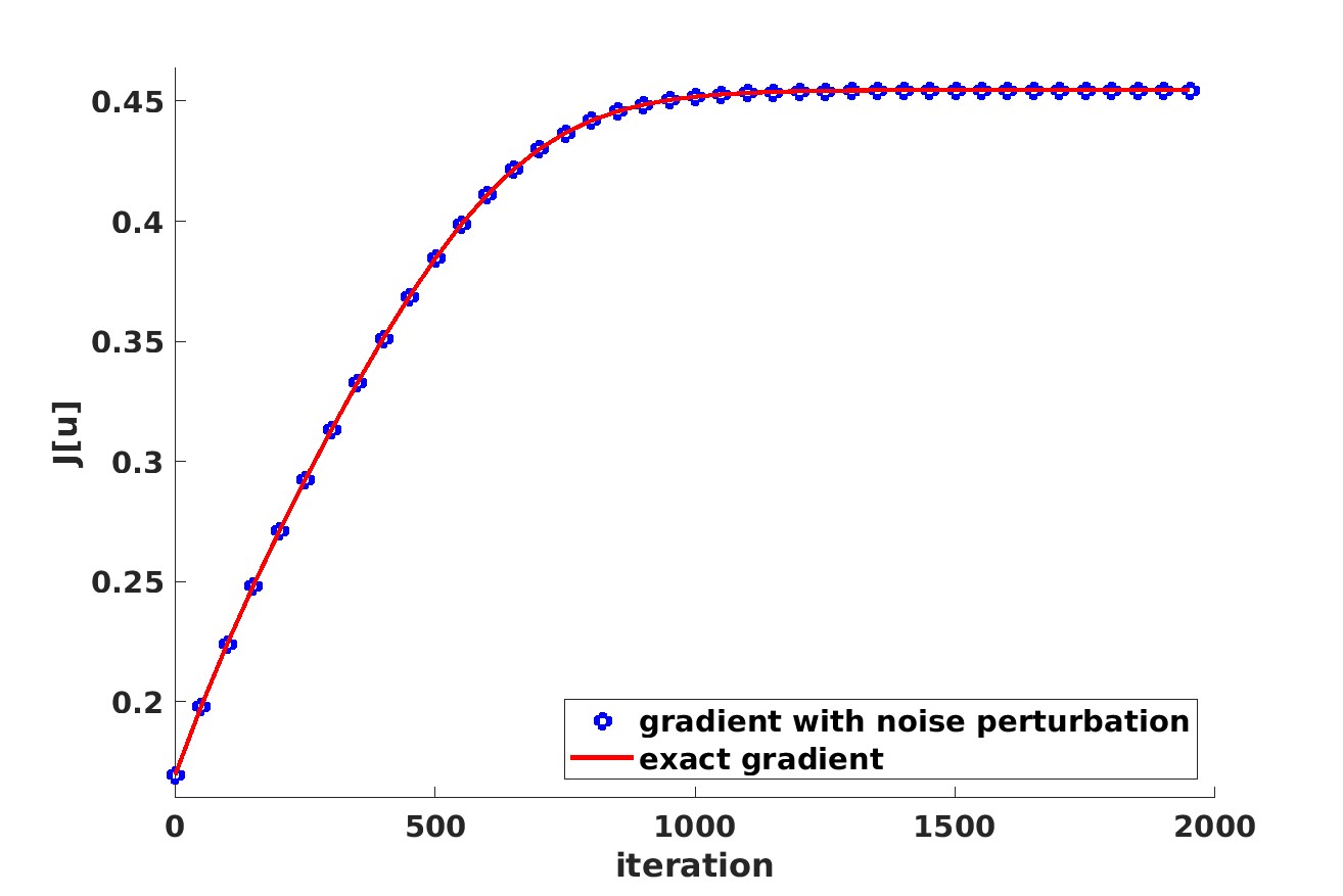
Figure 1: The loss function during 2000 iterations.

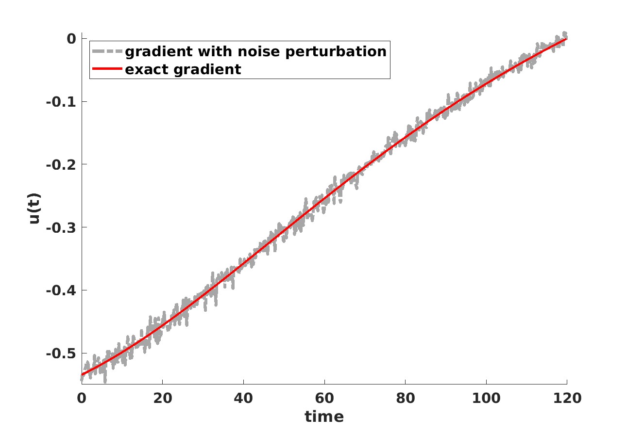
Figure 2: The control function after 2000 iterations.

6 Acknowledgements

We thank the anonymous reviewers for the valuable comments. We are also grateful to Wenhao He for pointing out a miscalculation of the gate complexity in an earlier version of this paper. XL’s research is supported by the National Science Foundation Grants DMS-2111221. CW acknowledges support from National Science Foundation grant CCF-2238766 (CAREER). Both XL and CW were supported by a seed grant from the Institute of Computational and Data Science (ICDS).

Appendix A The proof of Lemma 3.5

Proof.

To understand how the objective function $J$ depends on the control variables, we first explicitly write the piecewise-linear interpolating function using shape functions $b_{j}(t)$,

$$u_{I}(t)=\sum_{j}u_{j}b_{j}(t),$$

where $b_{j}(t)$’s are standard hat functions. We first examine the derivatives of $\ket{\psi(T)}$ with respect to the control variables. Following the TDSE in Eq. 1, we can write the derivative of $\psi(t)$ with respect to $u_{j}$, $\phi_{1}(t)\coloneqq\partial_{u_{j}}\psi(t),$ as follows,

$$i\partial_{t}\phi_{1}=H(t)\phi_{1}-\mu b_{j}(t)\psi(t).$$ (37)

Known as a variational equation [17], such an equation characterizes the dependence of the solution on the parameters in an evolution equation. By using variation-of-constant formula, we find

$$\phi_{1}(t)=i\int_{0}^{t}U(t,t^{\prime})\mu\psi(t^{\prime})b_{j}(t^{\prime})\,\differential t^{\prime},$$

where $U(t,t^{\prime})$ is the unitary operator generated by $H(t).$ A straightforward bound thus follows,

$$\norm{\phi(t)}\leq\norm{\mu}\delta,\;\forall 0\leq t\leq T.$$

Here we used the fact that

$$\int_{0}^{T}\absolutevalue{b_{j}(t)}\,\differential t\leq\delta.$$

We can continue with this calculation by letting $\phi_{2}(t)\coloneqq\partial_{u_{j}}\phi_{1}(t)$ for a second order derivative:

$$i\partial_{t}\phi_{2}=H(t)\phi_{2}-2\mu b_{j}(t)\phi_{1}(t).$$

Therefore, $\norm{\phi_{2}(t)}\leq 2(\delta\norm{\mu})^{2}.$ Mixed derivatives can be treated similarly and they follow a similar bound. By defining $\phi_{3}(t)\coloneqq\partial_{u_{j}}\phi_{2}(t)$, we obtain,

$$i\partial_{t}\phi_{3}=H_{0}\phi_{3}-3\mu b_{j}(t)\phi_{2}(t).$$

By repeating this argument for higher-order derivatives, we arrive at the inequality.

$$\norm{\frac{\partial^{\bm{\alpha}}}{\partial u_{\alpha_{1}}u_{\alpha_{2}}\cdots u_{\alpha_{k}}}\psi(T)}\leq k!\left(\delta\|\mu\|\right)^{k}.$$ (38)

Consequently, the function $\widetilde{J}_{1}$ has derivative bounds,

$$\norm{\frac{\partial^{\bm{\alpha}}\widetilde{J}_{1}}{\partial u_{\alpha_{1}}u_{\alpha_{2}}\cdots u_{\alpha_{k}}}}\leq\sum_{j=0}^{k}\binom{k}{j}(k-j)!j!\left(\delta\|\mu\|\right)^{k}\leq(k+1)!\left(\delta\|\mu\|\right)^{k}.$$ (39)

∎

Appendix B Proof of Lemma 3.7

Proof.

First observe that $\widetilde{J}_{1}(\bm{u})$ depends on $\bm{u}$ smoothly. By Lemma 3.5, we have

$$B=\absolutevalue{\nabla_{\bm{r}}^{2m+1}J}=\mathcal{O}((2m+1)!\delta^{2m+1}).$$ (40)

Therefore, according to Lemma 3.6, the query complexity to achieve the error bound in the spectral norm is

$$\widetilde{\mathcal{O}}\left(\frac{N}{\epsilon}\frac{B^{\frac{1}{2m}}N^{\frac{1}{4m}}}{\epsilon^{\frac{1}{2m}}}\right).$$ (41)

We notice that by Stirling’s approximation,

$$(2m+1)!\approx\left(\frac{2m+1}{e}\right)^{2m+1}.$$ (42)

Therefore, it suffices to choose

$$m=\mathcal{O}\left(\frac{\log(T^{1/2}/\epsilon^{3/4})}{\log\log(T^{1/2}/\epsilon^{3/4})}\right),$$ (43)

so that both $m$ and $(T^{1/2}/\epsilon^{3/4})^{1/(2m)}$ are poly-logarithmic factors. As a result, we have the claimed query complexity. ∎

Appendix C The function ascent property Eq. 32

We start by noticing that,

$$J(\bm{u}^{(k+1)}) \geq J(\bm{u}^{(k)})+\left(\nabla J(\bm{u}^{(k)}),\bm{u}^{(k+1)}-\bm{u}^{(k)}\right)-\frac{L}{2}\norm{\bm{u}^{(k+1)}-\bm{u}^{(k)}}^{2}$$

$$\geq J(\bm{u}^{(k)})+\eta\norm{\nabla J(\bm{u}^{(k)})}^{2}+\eta\left(\nabla J(\bm{u}^{(k)}),\bm{\zeta}_{k}+\bm{e}_{k}\right)-\frac{\eta}{2}\norm{\nabla J(\bm{u}^{(k)})+\bm{e}_{k}+\bm{\zeta}_{k}}^{2}$$

$$\geq J(\bm{u}^{(k)})+\frac{\eta}{2}\norm{\nabla J(\bm{u}^{(k)})}^{2}-\eta\norm{\bm{\zeta_{k}}}^{2}-\eta\norm{\bm{e}_{k}}^{2}.$$

The first line was obtained from the Lipschitz condition on the gradient. Eq. 31 is then used to arrive at the second line.

By a telescoping sum, we arrive at the desired function ascent property,

$$J(\bm{u}^{(k)})\geq J(\bm{u}^{(0)})+\frac{\eta}{2}\sum_{j=0}^{k-1}\norm{\nabla J(\bm{u}^{(j)})}^{2}$$ (44)

$$\quad-\eta\sum_{j=0}^{k-1}\norm{\bm{\zeta_{j}}}^{2}-\eta\sum_{j=0}^{k-1}\norm{\bm{e_{j}}}^{2}.$$

The noise term $\sum_{j=0}^{k-1}\norm{\bm{\zeta_{j}}}^{2}$ has been treated probabilistically in [29] using a concentration inequality [28], which provides a bound of $\frac{1}{8}k\epsilon^{2}$ with high probability. Meanwhile, we set a failure probability $\rho=\nu/k$ in the gradient estimation such that,

$$\mathbb{P}\big{(}\norm{\bm{e}_{j}}^{2}<\epsilon^{2}/8\big{)}\geq(1-\rho),$$

implying that

$$\mathbb{P}\big{(}\norm{\bm{e}_{j}}^{2}<\epsilon^{2}/8,\;\forall 1\leq j\leq k\big{)}\geq(1-\rho)^{k}\geq 1-\nu.$$ (45)

References

- [1] Francesca Albertini and Domenico D’Alessandro. The Lie algebra structure and controllability of spin systems. Linear Algebra and its Applications, 350(1-3):213–235, July 2002.
- [2] Leonardo Banchi and Gavin E Crooks. Measuring analytic gradients of general quantum evolution with the stochastic parameter shift rule. Quantum, 5:386, 2021.
- [3] Dominic W Berry, Andrew M Childs, Aaron Ostrander, and Guoming Wang. Quantum algorithm for linear differential equations with exponentially improved dependence on precision. Communications in Mathematical Physics, 356(3):1057–1081, 2017.
- [4] Dominic W Berry, Andrew M Childs, Yuan Su, Xin Wang, and Nathan Wiebe. Time-dependent Hamiltonian simulation with -norm scaling. Quantum, 4:254, 2020.
- [5] Constantin Brif, Raj Chakrabarti, and Herschel Rabitz. Control of quantum phenomena: past, present and future. New Journal of Physics, 12(7):075008, July 2010.
- [6] A. Castro, J. Werschnik, and E. K. U. Gross. Controlling the Dynamics of Many-Electron Systems from First Principles: A Combination of Optimal Control and Time-Dependent Density-Functional Theory. Physical Review Letters, 109(15), October 2012.
- [7] Alberto Castro, Miguel AL Marques, and Angel Rubio. Propagators for the time-dependent kohn–sham equations. The Journal of chemical physics, 121(8):3425–3433, 2004.
- [8] Marco Cerezo, Andrew Arrasmith, Ryan Babbush, Simon C Benjamin, Suguru Endo, Keisuke Fujii, Jarrod R McClean, Kosuke Mitarai, Xiao Yuan, Lukasz Cincio, et al. Variational quantum algorithms. Nature Reviews Physics, 3(9):625–644, 2021.
- [9] Shantanav Chakraborty, András Gilyén, and Stacey Jeffery. The power of block-encoded matrix powers: Improved regression techniques via faster Hamiltonian simulation. In Proceedings of the 46th International Colloquium on Automata, Languages, and Programming (ICALP 2019), 2019.
- [10] Andrew M Childs and Jin-Peng Liu. Quantum spectral methods for differential equations. arXiv preprint arXiv:1901.00961, 2019.
- [11] Alexandre Choquette, Agustin Di Paolo, Panagiotis Kl Barkoutsos, David Sénéchal, Ivano Tavernelli, and Alexandre Blais. Quantum-optimal-control-inspired ansatz for variational quantum algorithms. Physical Review Research, 3(2):023092, 2021.
- [12] G. Ciaramella, A. Borzì, G. Dirr, and D. Wachsmuth. Newton Methods for the Optimal Control of Closed Quantum Spin Systems. SIAM Journal on Scientific Computing, 37(1):A319–A346, January 2015.
- [13] Gavin E Crooks. Gradients of parameterized quantum gates using the parameter-shift rule and gate decomposition. arXiv preprint arXiv:1905.13311, 2019.
- [14] Domenico D’Alessandro. Topological properties of reachable sets and the control of quantum bits. Systems & Control Letters, 41(3):213–221, October 2000.
- [15] Domenico D’Alessandro. Introduction to quantum control and dynamics. Chapman & Hall/CRC applied mathematics and nonlinear science series. Chapman & Hall/CRC, Boca Raton, 2008. OCLC: ocn123539646.
- [16] Supriyo Datta. Quantum transport: Atom to transistor. Cambridge University Press, 2005.
- [17] Peter Deuflhard and Folkmar Bornemann. Scientific computing with ordinary differential equations, volume 42. Springer Science & Business Media, 2002.
- [18] W. E, J. Han, and Q. Li. A mean-field optimal control formulation of deep learning. Res. Math. Sci., 6:1–41, 2019.
- [19] Reuven Eitan, Michael Mundt, and David J. Tannor. Optimal control with accelerated convergence: Combining the Krotov and quasi-Newton methods. Physical Review A, 83(5), May 2011.
- [20] Edward Farhi, Jeffrey Goldstone, and Sam Gutmann. A quantum approximate optimization algorithm. arXiv preprint arXiv:1411.4028, 2014.
- [21] Xiaozhen Ge, Rebing Wu, and Herschel Rabitz. Optimization landscape of quantum control systems. Complex System Modeling and Simulation, 1(2):77–90, 2021.
- [22] D Geppert, L Seyfarth, and R de Vivie-Riedle. Laser control schemes for molecular switches. Appl. Phys. B, 79(8):987–992, 2004.
- [23] András Gilyén, Srinivasan Arunachalam, and Nathan Wiebe. Optimizing quantum optimization algorithms via faster quantum gradient computation. In Proceedings of the Thirtieth Annual ACM-SIAM Symposium on Discrete Algorithms, pages 1425–1444. SIAM, 2019.
- [24] András Gilyén, Yuan Su, Guang Hao Low, and Nathan Wiebe. Quantum singular value transformation and beyond: exponential improvements for quantum matrix arithmetics. In Proceedings of the 51st Annual ACM SIGACT Symposium on Theory of Computing, pages 193–204. ACM, 2019.
- [25] Steffen J. Glaser, Ugo Boscain, Tommaso Calarco, Christiane P. Koch, Walter Köckenberger, Ronnie Kosloff, Ilya Kuprov, Burkhard Luy, Sophie Schirmer, Thomas Schulte-Herbrüggen, Dominique Sugny, and Frank K. Wilhelm. Training Schrödinger’s cat: quantum optimal control: Strategic report on current status, visions and goals for research in Europe. The European Physical Journal D, 69(12), December 2015.
- [26] K. He, X. Zhang, S. Ren, and J. Sun. Deep residual learning for image recognition. In Proc. IEEE Comput. Soc. Conf. Comput. Vis. Pattern Recognit., pages 770–778, 2016.
- [27] Maria Hellgren, Esa Räsänen, and E. K. U. Gross. Optimal control of strong-field ionization with time-dependent density-functional theory. Physical Review A, 88(1), July 2013.
- [28] Chi Jin, Praneeth Netrapalli, Rong Ge, Sham M Kakade, and Michael I Jordan. A short note on concentration inequalities for random vectors with subgaussian norm. arXiv preprint arXiv:1902.03736, 2019.
- [29] Chi Jin, Praneeth Netrapalli, Rong Ge, Sham M Kakade, and Michael I Jordan. On nonconvex optimization for machine learning: Gradients, stochasticity, and saddle points. Journal of the ACM (JACM), 68(2):1–29, 2021.
- [30] Stephen P Jordan. Fast quantum algorithm for numerical gradient estimation. Physical Review Letters, 95(5):050501, 2005.
- [31] Mária Kieferová, Artur Scherer, and Dominic W Berry. Simulating the dynamics of time-dependent hamiltonians with a truncated dyson series. Physical Review A, 99(4):042314, 2019.
- [32] David Kincaid, David Ronald Kincaid, and Elliott Ward Cheney. Numerical analysis: mathematics of scientific computing, volume 2. American Mathematical Soc., 2009.
- [33] Oleksandr Kyriienko and Vincent E Elfving. Generalized quantum circuit differentiation rules. Physical Review A, 104(5):052417, 2021.
- [34] Martin Larocca, Piotr Czarnik, Kunal Sharma, Gopikrishnan Muraleedharan, Patrick J Coles, and Marco Cerezo. Diagnosing barren plateaus with tools from quantum optimal control. Quantum, 6:824, 2022.
- [35] Martin Larocca, Nathan Ju, Diego García-Martín, Patrick J Coles, and Marco Cerezo. Theory of overparametrization in quantum neural networks. arXiv preprint arXiv:2109.11676, 2021.
- [36] Jiaqi Leng, Yuxiang Peng, Yi-Ling Qiao, Ming Lin, and Xiaodi Wu. Differentiable analog quantum computing for optimization and control. In Advances in Neural Information Processing Systems, 2022.
- [37] Jun Li, Xiaodong Yang, Xinhua Peng, and Chang-Pu Sun. Hybrid quantum-classical approach to quantum optimal control. Physical review letters, 118(15):150503, 2017.
- [38] Guang Hao Low and Isaac L Chuang. Hamiltonian simulation by qubitization. Quantum, 3:163, 2019.
- [39] Guang Hao Low and Nathan Wiebe. Hamiltonian simulation in the interaction picture. arXiv preprint arXiv:1805.00675, 2018.
- [40] Shai Machnes, Elie Assémat, David Tannor, and Frank K Wilhelm. Tunable, flexible, and efficient optimization of control pulses for practical qubits. Physical review letters, 120(15):150401, 2018.
- [41] Yvon Maday and Gabriel Turinici. New formulations of monotonically convergent quantum control algorithms. The Journal of Chemical Physics, 118(18):8191–8196, May 2003.
- [42] Richard L McCreery, Haijun Yan, and Adam Johan Bergren. A critical perspective on molecular electronic junctions: there is plenty of room in the middle. Phys. Chem. Chem. Phys., 15(4):1065–1081, 2013.
- [43] Yurii Nesterov. Lectures on convex optimization, volume 137. Springer, 2018.
- [44] Michael A Nielsen and Isaac Chuang. Quantum Computation and Quantum Information. Cambridge University Press, 2010.
- [45] Yao Song, Junning Li, Yong-Ju Hai, Qihao Guo, and Xiu-Hao Deng. Optimizing quantum control pulses with complex constraints and few variables through autodifferentiation. Physical Review A, 105(1):012616, 2022.
- [46] J. Werschnik and E. K. U. Gross. Quantum Optimal Control Theory. arXiv:0707.1883 [quant-ph], July 2007. arXiv: 0707.1883.
- [47] David Wierichs, Josh Izaac, Cody Wang, and Cedric Yen-Yu Lin. General parameter-shift rules for quantum gradients. Quantum, 6:677, 2022.
- [48] Zhi-Cheng Yang, Armin Rahmani, Alireza Shabani, Hartmut Neven, and Claudio Chamon. Optimizing variational quantum algorithms using pontryagin’s minimum principle. Physical Review X, 7(2):021027, 2017.
- [49] Yi Zhou, Junjie Yang, Huishuai Zhang, Yingbin Liang, and Vahid Tarokh. Sgd converges to global minimum in deep learning via star-convex path. In International Conference on Learning Representations, 2018.
- [50] Wusheng Zhu and Herschel Rabitz. A rapid monotonically convergent iteration algorithm for quantum optimal control over the expectation value of a positive definite operator. J.Chem. Phys., 109(2):385–391, 1998.
- [51] Wusheng Zhu and Herschel Rabitz. A rapid monotonically convergent iteration algorithm for quantum optimal control over the expectation value of a positive definite operator. The Journal of Chemical Physics, 109(2):385–391, July 1998.