Efficient Gradient-based Optimization for Reconstructing Binary Images in Applications to Electrical Impedance Tomography

Abstract

A novel and highly efficient computational framework for reconstructing binary-type images suitable for models of various complexity seen in diverse biomedical applications is developed and validated. Efficiency in computational speed and accuracy is achieved by combining the advantages of recently developed optimization methods that use sample solutions with customized geometry and multiscale control space reduction, all paired with gradient-based techniques. The control space is effectively reduced based on the geometry of the samples and their individual contributions. The entire 3-step computational procedure has an easy-to-follow design due to a nominal number of tuning parameters making the approach simple for practical implementation in various settings. Fairly straightforward methods for computing gradients make the framework compatible with any optimization software, including black-box ones. The performance of the complete computational framework is tested in applications to 2D inverse problems of cancer detection by electrical impedance tomography (EIT) using data from models generated synthetically and obtained from medical images showing the natural development of cancerous regions of various sizes and shapes. The results demonstrate the superior performance of the new method and its high potential for improving the overall quality of the EIT-based procedures.

Keywords: binary-type images $\circ$ electrical impedance tomography $\circ$ cancer detection problem $\circ$ gradient-based optimization $\circ$ PDE-constrained optimal control $\circ$ control space parameterization $\circ$ noisy measurements

1 Introduction

In this paper, we propose a novel computational approach for the optimal reconstruction of biomedical images to assist with the recognition of cancer-affected regions while solving an inverse problem of cancer detection (IPCD). The main focus is on applying our new approach to be aligned with the electrical impedance tomography (EIT) technique. However, one could easily extend this methodology to a broad range of problems in biomedical sciences, physics, geology, chemistry, etc. EIT is a rapidly developing non-invasive imaging technique gaining popularity during the last few decades by enabling various medical applications to perform screening for cancer detection [33, 11, 3, 5, 28, 25, 1]. This technique uses a well-known fact that the electrical properties of different tissues, e.g., electrical conductivity or permittivity, are different if they are healthy or affected by cancer. This phenomenon allows EIT to produce images of biological tissues by interpreting their response to applied electrical voltages (potentials) or injected currents [11, 16, 5]. More specifically, the inverse EIT problem reconstructs the electrical conductivity by measuring voltages or currents at electrodes placed on the surface of the tested medium. This so-called Calderon-type inverse problem [15] is highly ill-posed; we refer the reader to Borcea’s topical review paper [10]. Since the 1980s, various computational techniques have been suggested to solve this highly nonlinear inverse problem computationally; see the recent review papers [4, 9, 31] on the current state of the art and existing open problems associated with EIT and its applications.

Our particular interest is in creating a robust and computationally efficient EIT-based optimization framework that is useful in various applications for medical practices dealing with models characterized by parameters close to binary-type distributions such as electrical conductivity. Recent papers [2, 23, 17] propose to convert the inverse EIT statement into a PDE-constrained optimal control framework and apply multilevel control space reduction at various scales to improve the quality of the obtained binary images. In [7, 6], the authors proposed a novel (although fairly simple) computing algorithm built around a derivative-free optimization supported by a set of sample solutions. These samples are generated synthetically with a geometry based on some prior knowledge of the simulated phenomena and the expected structure of obtained images. Although the ease of parallelization allows operations on very large sample sets, enabling the best approximations for the initial guess, practical applications may be limited to reconstructions of cancerous spots bearing simple geometry, e.g., with circular shapes. This algorithm also requires some prior knowledge of the simulated phenomena in the form of approximated properties (electrical conductivity) for healthy tissues and regions affected by cancer.

In the current work, we propose a generalized 3-step optimization procedure that removes these limitations, making the computational framework applicable to models of various levels of complexity. The superior performance of this generalized methodology is achieved by adding the following new computational components.

1. We designed new methods for computing gradients and validating their correctness to further enhance the computational performance at Step 2, as discussed in Section 3.3. These gradients are computed with respect to all control variables used in the main optimization cycle (all three steps).

2. We also discussed the applicability of various gradient-based methods (optimizers) to further enhance the optimization performance.

3. The limitations of our simplified 2-step approach presented in [7, 6] are overcome by the addition of a new (third) step in the current procedure, namely a binary tuning optimization, as discussed in Section 3.4. We applied the multiscale-based post-processing filtering [18, 17] at the coarse scale to further enhance the quality of images obtained as the final output of our new optimization procedure.

The proposed computational framework has an easy-to-follow design split into three phases and tuned by a nominal (meaning, minimal) number of computational parameters making the approach simple for practical implementation for various applications far beyond biomedical imaging. We tested the performance of our new algorithm computationally in applications to 2D inverse problems of cancer detection using noisy data generated synthetically and obtained from medical images showing cancerous regions of various sizes and shapes developed naturally in the human body.

This paper proceeds as follows. Section 2 presents a general mathematical description of the inverse EIT problem formulated as an optimal control problem. The entire computational procedure for solving this optimization problem is discussed in Section 3. Model descriptions and detailed computational results, including a discussion of chosen methods, are presented in Section 4. Concluding remarks are provided in Section 5.

2 Inverse EIT Problem

2.1 Mathematical Model for Optimization

As discussed at length in [2, 23, 7, 17], the inverse EIT problem is formulated as a PDE-constrained optimal control problem. Here, we note that while we refer to the control theory throughout the entire paper, in a very general sense, we can treat this formulation as an example of a PDE-constrained optimization problem defined for an open and bounded set (domain) $\Omega\subset\mathbb{R}^{n},\ n=2,3$, representing a body with electrical conductivity at point $x\in\Omega$ given by function $\sigma(x):\,\Omega\rightarrow\mathbb{R}_{+}$. In this paper, we use the so-called “voltage–to–current” model where voltages (electrical potentials) $U=(U_{\ell})_{\ell=1}^{m}\in\mathbb{R}^{m}$ are applied to $m$ electrodes $(E_{\ell})_{\ell=1}^{m}$ with contact impedances $(Z_{\ell})_{\ell=1}^{m}\in\mathbb{R}^{m}_{+}$ subject to the ground (zero potential) condition

$$\sum_{\ell=1}^{m}U_{\ell}=0.$$ (1)

These voltages initiate electrical currents $(I_{\ell})_{\ell=1}^{m}\in\mathbb{R}^{m}$ through the same electrodes $E_{\ell}$ placed at the periphery $\partial\Omega$ of domain $\Omega$. We compute the electrical currents

$$I_{\ell}=\int_{E_{\ell}}\sigma(x)\dfrac{\partial u(x)}{\partial n}\,ds,\quad\ell=1,\ldots,m$$ (2)

based on conductivity field $\sigma(x)$ and a distribution of electrical potential $u(x):\,\Omega\rightarrow\mathbb{R}$ obtained by solving the following elliptic problem

$$\bm{\nabla}\cdot\left[\sigma(x)\bm{\nabla}u(x)\right] =0, \quad x\in\Omega$$ (3a)

$$\dfrac{\partial u(x)}{\partial n} =0, \quad x\in\partial\Omega-\bigcup\limits_{\ell=1}^{m}E_{\ell}$$ (3b)

$$u(x)+Z_{\ell}\sigma(x)\dfrac{\partial u(x)}{\partial n} =U_{\ell}, \quad x\in E_{\ell},\ \ell=1,\ldots,m$$ (3c)

in which $n$ is an external unit normal vector on $\partial\Omega$. A complete description and analysis of electrode models used in electric current computed tomography may be found, e.g., in [26].

We set conductivity $\sigma(x)$ in (3) as a control variable (or optimization variable; see our remark at the beginning of this section) and formulate the inverse EIT (conductivity) problem [15] as a PDE-constrained optimal control problem [2] by considering least-square minimization of mismatches $\left(I_{\ell}-I_{\ell}^{*}\right)^{2}$, where $(I_{\ell}^{*})_{\ell=1}^{m}\in\mathbb{R}^{m}$ are measurements of electrical currents $I_{\ell}$. In addition, we have to mention a well-known fact that this inverse EIT problem to be solved in a discretized domain $\Omega$ is highly ill-posed. Therefore, we enlarge the data up to a size of $m^{2}$ by adding new measurements following the “rotation scheme” described in detail in [2] while keeping the size of the unknown parameters, i.e., elements in the discretized description for $\sigma(x)$, fixed. Having a new set of data $\mathcal{D}^{*}=\left\{I_{\ell}^{k*}\right\}_{\ell,k=1}^{m}$ and in light of the Robin condition (3c) used together with (2), we define a complete form of the cost functional

$$\mathcal{J}(\sigma)=\sum_{k=1}^{m}\sum_{\ell=1}^{m}\left[\int_{E_{\ell}}\dfrac{U^{k}_{\ell}-u^{k}(x;\sigma)}{Z_{\ell}}\,ds-I^{k*}_{\ell}\right]^{2}$$ (4)

for the optimal control problem

$$\hat{\sigma}(x)=\underset{\sigma}{\operatorname{argmin}}\ \mathcal{J}(\sigma)$$ (5)

subject to PDE constraint as each function $u^{k}(\cdot;\sigma),\ k=1,\ldots,m$, solves elliptic PDE (forward EIT) problem (3). Here, we assume that optimal solution $\hat{\sigma}(x)$ in (5) is unique. We also note that after applying (2) and adding some noise, these solutions may be used for generating various model examples (synthetic data) for inverse EIT problems to adequately mimic the presence of regions affected by cancer we mentioned above.

2.2 Solution by Sample-based Parameterization

In the view of the binary type of a solution we seek to reconstruct, we assume that the actual (true) electrical conductivity $\sigma_{true}(x)$ is represented by

$$\sigma_{true}(x)=\left\{\begin{aligned} \sigma_{c},&\quad x\in\Omega_{c},\\ \sigma_{h},&\quad x\in\Omega_{h},\end{aligned}\right.\quad\Omega_{c}\cap\Omega_{h}=\emptyset,$$ (6)

where $\sigma_{c}$ and $\sigma_{h}$ are some constants for the respective cancer-affected region $\Omega_{c}$ and the healthy tissue part $\Omega_{h}$. As such, we seek the solution of (5) in a form of the linear (convex) combination

$$\sigma(x)=\sum_{i=1}^{N_{s}}\alpha_{i}\bar{\sigma}_{i}(x),\qquad 0\leq\alpha_{i}\leq 1,\qquad\sum_{i=1}^{N_{s}}\alpha_{i}=1,$$ (7)

where $\bar{\sigma}_{i}(x)$, $i=1,\ldots,N_{s}$, are sample solutions generated synthetically based on a general assumption for the solution structure provided in (6); see Section 3.1 for details. The proposed computational algorithm for solving optimization problem (5) could be executed in three steps and requires a preprocessing phase (Step 0), as shown briefly below and detailed in Section 3.

• Preprocessing includes choosing (approximating) constants $\sigma_{c}$ and $\sigma_{h}$ in (6), deciding on the geometry of sample solutions $\bar{\sigma}_{i}$, and generating a collection $\mathcal{C}(N)$ of $N$ samples with corresponding “measurements” obtained by using (2)–(3); see Section 3.1 for details.

• The initial basis of samples

  $$\mathcal{B}^{0}=\left\{\bar{\sigma}_{i}(x)\right\}_{i=1}^{N_{s}}\subset\mathcal{C}(N)$$ (8)

  is defined by choosing the $N_{s}$ “best” samples out of $\mathcal{C}(N)$ that provide the best measurement fit in terms of cost functional (4) (we elaborate more on this initialization procedure in Section 3.2). This basis will serve as the initial guess for the fine-scale optimization performed in Step 2.

• All parameters in the description of basis $\mathcal{B}^{0}$ and weights $\alpha_{i}$ in (7)–(8) are set as controls to perform gradient-based optimization for solving problem (5) numerically to find the optimal solution $\hat{\sigma}(x)$ at a fine scale (i.e., using a fine mesh on which we reconstruct images for electrical conductivity $\sigma(x)$) via optimal control set $(\hat{\mathcal{B}},\hat{\alpha})$ as shown in Section 3.3.

• The fine-scale optimal solution $\hat{\sigma}(x)$ is then finally tuned to create an optimal binary image $\hat{\sigma}_{b}(x)$ by moving $\hat{\sigma}(x)$ from the fine to the coarse scale (where $\hat{\sigma}_{b}(x)$ leaves) using a multiscale optimization algorithm. Here, we use the “coarse scale” notation to refer to an upscaled (reduced-dimensional) control space containing just a few controls representing reconstructed values for high and low electrical conductivities inside each cancerous region and outside, respectively. In short, this step will tune the fine-scale solution obtained in Step 2 by recreating it as a piecewise constant reconstruction; refer to Section 3.4 for more details.

To comment more on the “philosophy” behind the entire approach, we would reiterate that the fine-scale optimization of Step 2 is used to approximate the location of regions with high and low values of electrical conductivity $\sigma(x)$, and projecting obtained solutions onto the coarse scale in Step 3 provides a dynamical (sharp-edge) filtering to the fine-scale images optimized to better represent the structure of the cancer-affected regions (i.e., their location and boundaries).

3 Gradient-based Optimization Framework

3.1 Step 0: Sample Preprocessing

Without loss of generality, in this paper, we discuss the application of the new algorithm to solving optimization problem (5) in the 2D ($n=2$) domain, e.g.,

$$\Omega=\left\{x\in\mathbb{R}^{2}:\ \|x\|^{2}<R^{2}\right\},$$ (9)

which is a disc of radius $R$. However, the same concept could be easily extended to 3D ($n=3$) regions of various complexity.

The entire collection of $N$ samples

$$\mathcal{C}(N)=\left\{\bar{\sigma}_{i}(x)\right\}_{i=1}^{N},\qquad N\gg N_{s}$$ (10)

could be generated based on various assumptions made for the (geometrical) structure of the reconstructed images with the binary type restriction. Here, we assume that flexibility in reconstructing images of various complexity and also convenient simplicity could be achieved by combining simple convex geometric shapes (elements) in 2D such as triangles, squares, circles, etc. For example, in this paper, the $i$th sample in $\mathcal{C}(N)$ consists of $N_{c}^{i}$ circles of various radii $r\in\mathbb{R}_{+}$ and centers $x^{0}=(x^{01},x^{02})\in\mathbb{R}^{2}$ located inside domain $\Omega$, i.e.,

$$\bar{\sigma}_{i}(x)=\left\{\begin{aligned} \tilde{\sigma}_{c},&\quad\mid x-x^{0}_{j}\mid^{2}\leq r^{2}_{j},\quad j=1,\ldots,N_{c}^{i}\\ \tilde{\sigma}_{h},&\quad{\rm otherwise}\end{aligned}\right.$$ (11)

where some approximations $\tilde{\sigma}_{c}$ and $\tilde{\sigma}_{h}$ for respective $\sigma_{c}$ and $\sigma_{h}$ in (6) are required and considered as a priori knowledge needed for applying the approach in practice. In (11), all $N_{c}^{i}$ circles (i.e., cancer-affected regions) are parameterized by the set of triplets

$$\mathcal{P}_{i}=\left\{(x^{01}_{j},x^{02}_{j},r_{j})\right\}_{j=1}^{N_{c}^{i}},\qquad i=1,\ldots,N$$ (12)

generated randomly subject to the following restrictions

$$\mid x^{0}_{j}\mid<R+r_{j},\qquad j =1,\ldots,N_{c}^{i},$$ (13)

$$1\leq N_{c}^{i}\leq N_{c,\max},\qquad i =1,\ldots,N.$$

Parameter $N_{c,\max}$ in (13) defines the maximum number of circles in the samples and, in fact, sets the highest level of complexity (resolution) for the reconstructed images (refer to [6, 7] for more details on technicalities of this preprocessing step).

Finalizing the preprocessing procedure requires solving forward problem (3) and evaluating cost functional (4) $N$ times for all samples in $\mathcal{C}(N)$. Using a fixed scheme of potentials $U$, the entire “measurement” data $\mathcal{D}=\left\{\mathcal{D}_{i}\right\}_{i=1}^{N}$, where $\mathcal{D}_{i}=I^{k}_{\ell}(\bar{\sigma}_{i})\in\mathbb{R}^{m^{2}}$, are precomputed by (2)–(3) and then stored for multiple uses with different models. In addition, this task may run in parallel with minimal computational overhead, which allows easy switching between various schemes for electrical potentials. Easy parallelization enables taking $N$ to be quite large, which helps better approximate the solution by the initial state of basis $\mathcal{B}$ during Step 1 before proceeding to Step 2.

3.2 Step 1: Initializing Sample Basis

We set the number of samples $N_{s}$ in the initial basis $\mathcal{B}^{0}$ as a hyper parameter of the algorithm and define it heuristically after making assumptions on the model complexity or after experimentation. We suggest $N_{s}$ be sufficiently large to properly support a local/global search for optimal solution $\hat{\sigma}(x)$ during Step 2. At the same time, while solving problem (5), this number should allow the total number of controls, to be comparable with the size of the data, namely $m^{2}$, for satisfying the well-posedness requirement for the solution of the optimization problem in the sense of Hadamard [21].

Considering models with highly complicated structures may require increasing the number of elements (in our case, circles) in every sample within the chosen basis $\mathcal{B}^{0}$. In this case, one could re-set parameters $N_{c}^{i},\ i=1,\ldots,N_{s}$, to higher values and add missing elements, for example, by generating randomly new circles. It will project the initial basis $\mathcal{B}^{0}$ onto a new control space of a higher dimension to minimize the loss in the quality of the initial solution $\sigma(\mathcal{B}^{0},\alpha^{0})$.

Step 1 will be completed after ranking all samples in $\mathcal{C}(N)$ in ascending order using computed cost functionals (4) while comparing the obtained data $\mathcal{D}$ with true data $\mathcal{D}^{*}$ available from the actual measurements. After ranking, the first $N_{s}$ samples create the initial basis $\mathcal{B}^{0}$ to construct solution $\sigma(\mathcal{B}^{0},\alpha^{0})$ used as the initial guess for optimization in Step 2.

3.3 Step 2: Fine-Scale Gradient-based Optimization

As discussed in Section 3.1, all elements (circles) in all samples of basis $\mathcal{B}^{0}$ obtained during the Step 1 ranking procedure are represented by a finite number of “sample-based” parameters associated with set $\left\{\mathcal{P}_{i}\right\}_{i=1}^{N_{s}}$. In general, solution $\sigma(x)=\sigma(\mathcal{P},\alpha)$ could be uniquely represented as a function of set $\mathcal{P}=\left\{\mathcal{P}_{i}\right\}_{i=1}^{N_{s}}$ and vector of weights $\alpha=(\alpha_{i})_{i=1}^{N_{s}}$. We substitute the continuous form of optimal control problem (5) with its new equivalent form

$$(\hat{\mathcal{P}},\hat{\alpha})=\underset{\mathcal{P},\alpha}{\operatorname{argmin}}\ \mathcal{J}(\mathcal{P},\alpha)$$ (14)

to be solved numerically subject to PDE constraint (3), linear constraints for $\alpha_{i}$ in (7), and suitably established bounds for all components of the combined control set $(\mathcal{P},\alpha)$. As naturally followed from the structure of this new control, a dimension of the parameterized solution space is bounded by

$$\dim(\mathcal{P},\alpha)\leq N_{s}\cdot[N_{c,\max}(n+1)+1].$$ (15)

To solve (14) iteratively, one may choose various criteria to terminate the optimization run at the $k$th iteration, e.g., comparing the relative decrease in the cost functional $\mathcal{J}^{k}$ evaluated after completing $k$ iterations

$$\dfrac{\mid\mathcal{J}^{k}-\mathcal{J}^{k-1}\mid}{\mathcal{J}^{k}}<\epsilon,\qquad k>0$$ (16)

with preset tolerance $\epsilon\in\mathbb{R}_{+}$.

The prior works on using sample-based parameterization [7, 6] employed the coordinate descent (CD) method to solve (14). While achieving a good performance when applied to simple models, CD obviously exhibits certain limitations as it optimizes over a single control at a time. Without proper parallelization, it requires enormous cost functional evaluations and, as such, a large amount of computational time to complete optimization with the reasonably small $\epsilon$. Instead, our new optimization framework operates with fairly straightforward methods for computing gradients derived with respect to all controls in the control set $(\mathcal{P},\alpha)$.

We start our derivation of gradients relative to both sample-based parameters in set $\mathcal{P}$ and weights $\alpha$ by referring to the known structure [17, 23, 2] of gradients $\mathcal{J}^{\prime}_{\sigma}$ obtained with respect to control $\sigma$

$$\mathcal{J}^{\prime}_{\sigma}=-\sum_{k=1}^{m}\bm{\nabla}\psi^{k}(x)\cdot\bm{\nabla}u^{k}(x)$$ (17)

computed based on solutions $\psi^{k}(\cdot;\sigma):\,\Omega\rightarrow\mathbb{R},\ k=1,\ldots,m$, of the following adjoint PDE problem

$$\bm{\nabla}\cdot\left[\sigma(x)\bm{\nabla}\psi(x)\right] =0, \quad x\in\Omega$$ (18)

$$\dfrac{\partial\psi(x)}{\partial n} =0, \quad x\in\partial\Omega-\bigcup\limits_{\ell=1}^{m}E_{\ell}$$

$$\psi(x)+Z_{\ell}\dfrac{\partial\psi(x)}{\partial n} =2\beta_{\ell}\left[\int_{E_{\ell}}\dfrac{u(x)-U_{\ell}}{Z_{\ell}}\,ds+I^{*}_{\ell}\right], \quad x\in E_{\ell},$$

$$\quad\ell=1,\ldots,m$$

First, we derive the gradient $\bm{\nabla}_{\alpha}\mathcal{J}$ of cost functional $\mathcal{J}$ with respect to control $\alpha$. Using connectivity of solution $\sigma(x)$ with individual sample $\bar{\sigma}_{i}$ weights $\alpha_{i}$ provided explicitly by (7), partial derivatives

$$\dfrac{\partial\sigma(x)}{\partial\alpha_{i}}=\bar{\sigma}_{i},\quad i=1,\ldots,N_{s}$$ (19)

are then used to construct the gradient

$$\bm{\nabla}_{\alpha}\sigma=\left[\bar{\sigma}_{1}\ \bar{\sigma}_{2}\ \ldots\bar{\sigma}_{N_{s}}\right]^{T}\triangleq\bar{\sigma}.$$ (20)

Then using the chain rule gives the sought gradient

$$\bm{\nabla}_{\alpha}\mathcal{J}=\bm{\nabla}_{\alpha}\sigma\cdot\mathcal{J}^{\prime}_{\sigma}=\bar{\sigma}\cdot\mathcal{J}^{\prime}_{\sigma}.$$ (21)

We also note that in the discretized settings (when domain $\Omega$ undergoes $N_{\Omega}$-component discretization), $\bar{\sigma}$ and $\mathcal{J}^{\prime}_{\sigma}$ are represented by $N_{s}\times N_{\Omega}$ matrix and $N_{\Omega}$-component column-vector, respectively.

Finally, the gradient $\bm{\nabla}_{\mathcal{P}}\mathcal{J}$ of cost functional $\mathcal{J}$ with respect to sample-based control $\mathcal{P}$ is derived in the same manner by using the chain rule and precomputed gradient $\mathcal{J}^{\prime}_{\sigma}$

$$\bm{\nabla}_{\mathcal{P}}\mathcal{J}=\bm{\nabla}_{\mathcal{P}}\sigma\cdot\mathcal{J}^{\prime}_{\sigma}.$$ (22)

Deriving $\bm{\nabla}_{\mathcal{P}}\sigma$ appears complicated due to the involved geometry of $\sigma(\mathcal{P},\alpha)$ that may neither have a straightforward structure nor be known due to the randomness of the process described in (11)–(13). However, recent studies [29, 24] suggest a flexible approach when some partial derivatives used as a part of the adjoint-based analysis are approximated by numerical perturbations. We could conveniently adapt this approach as, in the current framework, it will not require reevaluating cost functionals: only changes in the sample solution $\bar{\sigma}_{i}$ associated with its own parameter $\mathcal{P}_{i}$ should be assessed. Thus, we perturb every parameter $\mathcal{P}_{i}$ in control set $\mathcal{P}$

$$\dfrac{\partial\sigma}{\partial\mathcal{P}_{i}}\approx\dfrac{\Delta\sigma}{\Delta\mathcal{P}_{i}}=\alpha_{i}\dfrac{\Delta\bar{\sigma}_{i}}{\Delta\mathcal{P}_{i}},\quad i=1,\ldots,N_{s}$$ (23)

by setting all perturbations $\Delta\mathcal{P}_{i}$ to numerical values pursuing a trade-off between being reasonably small to ensure the accuracy of finite-difference (FD) estimations of ${\partial\sigma}/{\partial\mathcal{P}_{i}}$ and large enough to protect the numerator from being zero.

3.4 Step 3: Coarse-Scale Binary Tuning Optimization

For the last step, we employ a recently designed gradient-based approach to support multiscale optimization with multilevel control space reduction using principal component analysis (PCA) coupled with dynamical control space upscaling [23, 17]. As pointed out before, this step introduces projecting the fine-scale solutions $\hat{\sigma}(x)$ onto the coarse scale (i.e., new upscaled control space with a significantly reduced number of controls) to perform a dynamical (sharp-edge) filtering to the fine-scale images. New images represented by the coarse-scale solutions $\hat{\sigma}_{b}(x)$ are optimized to better represent the structure of the cancer-affected regions (i.e., their location and boundaries). From the entire approach presented in [23, 17], we adopt only the coarse-scale phase to be applied to the fine-scale solution $\hat{\sigma}(x)$ obtained during Step 2.

First, we must specify the maximum (expected) number of cancer-affected (high conductivity) regions $N_{\max}$. By considering the healthy part (low conductivity region $\Omega_{h}$) of domain $\Omega$ as a single region, partitioning the fine mesh elements representing $\Omega$ will create $N_{\zeta}=N_{\max}+1$ spatial subsets. To proceed with Step 3 optimization at the coarse scale, we define a new control vector $\zeta=(\zeta_{j})_{j=1}^{2N_{\max}+1}$ of significantly reduced dimensionality, in which the first entry is the low value of (binary) electrical conductivity $\sigma(x)$ associated with a healthy region $\Omega_{h}$. The next $N_{\max}$ controls are the high values of $\sigma(x)$ related to areas in $\Omega_{c}$ affected by cancer, i.e.,

$$\zeta_{1}=\sigma_{low},\quad\zeta_{2}=\sigma_{high,1},\quad\zeta_{3}=\sigma_{high,2},\quad\ldots,\quad\zeta_{N_{\max}+1}=\sigma_{high,N_{\max}}.$$ (24)

The rest $N_{\max}$ components

$$\zeta_{N_{\max}+2}=\sigma_{th,1},\quad\zeta_{N_{\max}+3}=\sigma_{th,2},\quad\ldots,\quad\zeta_{2N_{\max}+1}=\sigma_{th,N_{\max}}$$ (25)

take responsibility for the shape of those $N_{\max}$ cancerous regions. They are set as separation thresholds to define boundaries between the low and high-conductivity areas. The structure of control $\zeta$ allows the creation of the systematic representation of the coarse-scale solution $\zeta^{k}$ for control $\sigma^{k}$ at the $k$th iteration based on the current fine-scale parameterization $\sigma(\zeta^{k})=(\sigma_{i}(\zeta^{k}))_{i=1}^{N_{\Omega}}$, i.e,

$$\sigma^{k}_{i}=\left\{\begin{aligned} \sigma^{k}_{low},&\quad\sigma_{i}(\zeta^{k})<\sigma^{k}_{th,n},\\ \sigma^{k}_{high,n},&\quad\sigma_{i}(\zeta^{k})\geq\sigma^{k}_{th,n},\end{aligned}\right.\quad i=1,\ldots,N_{\Omega},\quad 1\leq n\leq N_{\max}.$$ (26)

Here, $n=n(i)$ denotes the number of a particular cancer-affected region defined subject to the partitioning map currently established and used for the $k$th iteration [17]. We also note that

$$0<\sigma^{k}_{low} <\underset{1\leq n\leq N_{\max}}{\min}\ \sigma^{k}_{high,n},$$ (27)

$$\underset{1\leq i\leq N_{\Omega}}{\min}\ \sigma_{i}(\zeta^{k})<\sigma^{k}_{th,n} <\underset{1\leq i\leq N_{\Omega}}{\max}\ \sigma_{i}(\zeta^{k}),\quad n=1,\ldots,N_{\max}.$$

Simply, (26) provides a rule for creating a fine–to–coarse partition of discretized fine-scale solution $\hat{\sigma}$ with all spatial elements $\hat{\sigma}_{i}$ belonging either to cancer affected region $\Omega_{c}$ ($\hat{\sigma}_{i}=\sigma_{high,n}$, $n=1,\ldots N_{\max}$) or the healthy tissue part $\Omega_{h}$ ($\hat{\sigma}_{i}=\sigma_{low}$) based on the current state of control $\zeta^{k}$ (at the $k$th iteration).

During the Step 3 (coarse-scale optimization) phase, control $\sigma^{k}$ is updated by solving the following ($2N_{\max}+1$)-dimensional optimization problem in the $\zeta$-space

$$\hat{\zeta}=\underset{\zeta}{\operatorname{argmin}}\ \mathcal{J}(\zeta)$$ (28)

subject to constraints (bounds) provided in (27) and optimal (binary) solution $\hat{\sigma}_{b}(x)=\sigma(\hat{\zeta})$. To solve (28) by any approaches that require computing gradients, their first $N_{\max}+1$ components could be easily obtained by using a gradient summation formula derived in [23] and upgraded in [17] for the case of multiple cancer-affected regions

$$\dfrac{\partial\mathcal{J}(\zeta)}{\partial\zeta_{j}}=\sum_{i=1}^{N_{\Omega}}P_{i,j}\mathcal{J}^{\prime}_{\sigma,i}\Delta_{i},\quad j=1,\ldots,N_{\max}+1.$$ (29)

Here, $\mathcal{J}^{\prime}_{\sigma,i}$ is the $i$th component of the discretized gradient $\mathcal{J}^{\prime}_{\sigma}$, and $P_{i,j}$ is the partitioning (indicator) function defined by

$$P_{i,j}=\left\{\begin{aligned} 1,\quad\sigma_{i}&\in C_{j},\\ 0,\quad\sigma_{i}&\notin C_{j},\end{aligned}\right.$$ (30)

after completing the partitioning map by employing (26). In (30), $C_{1}$ is the current representation of the healthy region $\Omega_{h}$, and $C_{n+1}$, $n=1,\ldots,N_{\max}$, are parts of the cancerous area $\Omega_{c}$.

The rest $N_{\max}$ components may be approximated by a finite difference scheme, e.g., of the first order:

$$\dfrac{\partial\mathcal{J}(\zeta)}{\partial\zeta_{j}} =\dfrac{1}{\delta_{\zeta}}\left[\mathcal{J}\left(\sigma^{k}(\ldots,\zeta_{j}+\delta_{\zeta},\ldots)\right)-\mathcal{J}\left(\sigma^{k}(\ldots,\zeta_{j},\ldots)\right)\right]+\mathcal{O}(\delta_{\zeta}),$$ (31)

$$n =1,\ldots,N_{\max},\quad j=n+N_{\max}+1$$

which requires at most $N_{\max}$ extra cost functional evaluations per optimization iteration. Following the same discussion as in Section 3.3, parameter $\delta_{\zeta}$ in (31) may be defined experimentally, pursuing a trade-off between being reasonably small to ensure accuracy and large enough to protect the numerator from being zero.

In fact, formulas (26)–(28) provide a complete description of Step 3 fine–to–coarse projection (or, as we call it before, coarse-scale binary tuning) for fine-scale optimal control $\hat{\sigma}(x)$ to obtain optimal (in terms of fitting to data $\mathcal{D}^{*}$) binary distribution $\hat{\sigma}_{b}(x)$. An import remark should be made here for the performance of the binary tuning optimization of Step 3. As shown in multiple examples in [23, 17], the “quality” of the coarse-scale solution $\hat{\sigma}_{b}$ is usually worse compared to the quality of the fine-scale images $\hat{\sigma}$ if evaluated in terms of fitting to the same data $\mathcal{D}^{*}$. This effect is expected as the coarse scale operates with significantly reduced number of parameters (components of Step 3 control variable $\zeta$), reconstructing in fact piecewise constant representation of electrical conductivity $\sigma(x)$ after applying sharp-edge filtering to better represent the structure of the cancer-affected regions in terms of their location and boundaries. Such solutions could lose even more “quality” if the used data contains noise.

The efficiency of the entire optimization framework is confirmed by extensive computational results for multiple models of different complexity presented in Section 4. A summary of the complete computational framework to perform our new optimization with sample-based parameterization and multiscale control-space reduction for binary tuning is provided in Algorithm 1.

  set parameters: $N$, $N_{c,\max}$, $N_{s}$

   Step 0 Sample Preprocessing

  for $i\leftarrow 1$ to $N$ do

     generate $\bar{\sigma}_{i}(x)$ by (11)–(13)

     obtain data $\mathcal{D}_{i}=I^{k}_{\ell}(\bar{\sigma}_{i})$ from sample $\bar{\sigma}_{i}$ by (2)–(3)

  end for

   Step 1 Initializing Sample Basis

  select model and obtain true data $\mathcal{D}^{*}$

  for $i\leftarrow 1$ to $N$ do

     compute $\mathcal{J}(\bar{\sigma}_{i})$ by (4)

  end for

  choose $N_{s}$ best samples from $\mathcal{C}(N)$ by values $\mathcal{J}(\bar{\sigma}_{i})$

  form initial basis $\mathcal{B}^{0}$

  set initial weights $\alpha^{0}$

  compute $\sigma^{0}(x)$ using $\mathcal{B}^{0}$ and $\alpha^{0}$ by (7)

   Step 2 Fine-Scale Optimization

  $k\leftarrow 0$

  repeat

     compute state $u^{k}$ by solving (3)

     compute adjoint state $\psi^{k}$ by solving (18)

     compute gradient $\mathcal{J}^{\prime}_{\sigma}$ using (17)

     obtain gradients $\bm{\nabla}_{\mathcal{P}}\mathcal{J}$ and $\bm{\nabla}_{\alpha}\mathcal{J}$ respectively by (22)–(23) and (19)–(21)

     update control set $(\mathcal{P},\alpha)$ using gradients $\bm{\nabla}_{\mathcal{P}}\mathcal{J}$ and $\bm{\nabla}_{\alpha}\mathcal{J}$

     $k\leftarrow k+1$

     update $\sigma^{k}(x)$ using new basis $\mathcal{B}^{k}=\mathcal{B}(\mathcal{P}^{k})$ and weights $\alpha^{k}$ by (7)

  until termination criterion (16) is satisfied to given tolerance $\epsilon$

  obtain optimal solution $\hat{\sigma}(x)=\sigma(\hat{\mathcal{B}},\hat{\alpha})$

   Step 3 Coarse-Scale Binary Tuning

  $k\leftarrow 0$

  $\sigma^{0}_{i}\leftarrow(\hat{\sigma}_{i})_{i=1}^{N_{\Omega}}$

  define $\zeta^{0}$ by (26)–(27)

  repeat

     compute gradient $\bm{\nabla}_{\zeta}\mathcal{J}$ using (29)–(31)

     update control $\zeta$ using gradient $\bm{\nabla}_{\zeta}\mathcal{J}$

     $k\leftarrow k+1$

     update $\sigma_{i}^{k}$ using (26)

  until termination criterion (16) is satisfied to given tolerance $\epsilon$

  obtain optimal solution $\hat{\sigma}_{b}=\sigma_{i}(\hat{\zeta})$

Algorithm 1 Computational workflow for gradient-based optimization in binary images reconstruction

4 Computational Results

4.1 2D Model Setup

Our optimization framework integrates computational facilities for solving forward PDE problem (3), adjoint PDE problem (18), evaluating cost functionals by (4), and constructing gradients according to (17), (21), (22), and (29)–(31). These facilities are incorporated using FreeFEM [22], an open-source, high-level integrated development environment for obtaining numerical solutions of PDEs based on the finite element method (FEM). For solving numerically forward PDE problem (3), spatial discretization is carried out by implementing FEM triangular finite elements: P2 piecewise quadratic (continuous) and P0 piecewise constant representations for electrical potential $u(x)$ and conductivity field $\sigma(x)$, respectively. Systems of algebraic equations obtained after such discretization are solved with UMFPACK, a solver for nonsymmetric sparse linear systems [19]. The same technique is used for numerical solutions of adjoint problems (18).

All computations are performed using a 2D domain (9) which is a disc of radius $R=0.1$ with $m=16$ equidistant electrodes $E_{\ell}$ with half-width $w=0.12$ rad covering approximately 61% of boundary $\partial\Omega$ as shown in Figure 1(a). Electrical potentials

$$(U_{\ell})_{\ell=1}^{16}=\left\{-3,+1,+2,-5,+4,-1,-3,+2,+4,+3,-3,+3,+2,-4,+1,-3\right\}$$

are applied to electrodes $E_{\ell}$ following the “rotation scheme” discussed in Section 2.1 and chosen to be consistent with the ground potential condition (1). Figure 1(b) shows an example of the distribution of flux $\sigma(x)\bm{\nabla}u(x)$ of electrical potential $u$ in the interior of domain $\Omega$ and measured currents $(I_{\ell}^{*})_{\ell=1}^{16}$ during the EIT procedure. Determining the Robin part of the boundary conditions in (3c), we equally set the electrode contact impedance $Z_{\ell}=0.1$.

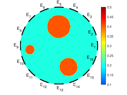
(a) model #1

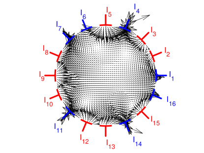
Figure 1: (a) EIT model #1: true electrical conductivity $\sigma_{true}(x)$ and equispaced geometry of electrodes $E_{\ell}$ placed over boundary $\partial\Omega$. (b) Electrical currents $I_{l}$ (positive in red, negative in blue) induced at electrodes $E_{\ell}$. Black arrows show the distribution of flux $\sigma(x)\bm{\nabla}u(x)$ of electrical potential $u$ in the interior of domain $\Omega$.

The actual (true) electrical conductivity $\sigma_{true}(x)$ we seek to reconstruct is defined analytically for each model in (6) by setting $\sigma_{c}=0.4$ and $\sigma_{h}=0.2$ unless stated otherwise. The initial guess for control $\mathcal{P}$ at Step 2 is provided by the parameterization of initial basis $\mathcal{B}^{0}$ obtained after completing Step 1. For control $\alpha$, the initial values are set to be equal, i.e., $\alpha^{0}_{i}=1/N_{s}$. The initial state of control $\zeta$ in Step 3 is approximated by

$$\sigma^{0}_{th,n} =\sigma_{ini}=\frac{1}{2}\left[\underset{1\leq i\leq N_{\Omega}}{\max}\ \sigma_{i}(\zeta^{0})+\underset{1\leq i\leq N_{\Omega}}{\min}\ \sigma_{i}(\zeta^{0})\right],$$ (32)

$$\sigma^{0}_{low} =\underset{1\leq i\leq N_{\Omega}}{\operatorname{mean}}\left\{\sigma_{i}(\zeta^{0}):\ \sigma_{i}(\zeta^{0})<\sigma_{ini}\right\},$$

$$\sigma^{0}_{high,n} =\underset{1\leq i\leq N_{\Omega}}{\operatorname{mean}}\left\{\sigma_{i}(\zeta^{0}):P_{i,n+1}=1,\ \sigma_{i}(\zeta^{0})\geq\sigma_{ini}\right\},$$

$$n =1,\ldots,N_{\max}.$$

Termination criteria are set by tolerance $\epsilon=10^{-9}$ in (16) and the total number of cost functional evaluations of 50,000, whichever is reached first.

For generating samples in $\mathcal{C}(N)$ collections discussed in Section 3.1, we use $N=10,000$ and $N_{c,max}=8$. This set is precomputed using a generator of uniformly distributed random numbers. Therefore, each sample $\bar{\sigma}_{i}(x)$ “contains” from one to eight “cancer-affected” areas with $\sigma_{c}=0.4$. Each area is located randomly within domain $\Omega$ and represented by a circle of randomly chosen radius $0<r\leq 0.3R$ as exemplified in Figure 2. Also, we fix the number of samples $N_{s}$ to 10 for all numerical experiments shown in this paper. Finally, the results of our previous research [7, 6] confirm that our sample-based parameterization enables high-level stability of the obtained results towards the noise present in measurements. Thus, for all numerical experiments shown in this paper, we use measurement data contaminated with $0.5\%$ normally distributed (Gaussian) noise.

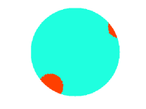
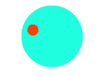
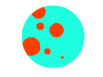
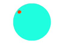
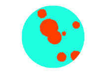
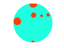
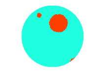
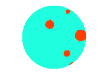
Figure 2: 8 first sample solutions $\bar{\sigma}_{i}(x),\,i=1,\ldots,8$, from the set $\mathcal{C}(10,000)$.

4.2 Optimization Framework Validation

To demonstrate the applicability of the proposed computational framework discussed in Section 3 and check its overall performance through a sequence of steps while solving the inverse EIT problem, we use model #1 featuring three circular-shaped cancerous regions of various sizes, as shown in Figure 1(a). We use this model to mimic a typical situation for a cancer-affected biological tissue containing several spots suspected of being tumorous and, as such, having elevated electrical conductivity.

4.2.1 Validating Gradients

The gradient-based concept is central to the proposed methodology; therefore, our first results demonstrate the consistency of the gradients computed for various controls (optimization variables), as discussed in Section 3.3. Figures 3 and 4 show the results of a diagnostic test ($\kappa$-test) commonly employed to verify the correctness of the discretized gradients; see, e.g., [14, 13, 17, 12]. It consists in computing the directional differential, e.g., $\mathcal{J}^{\prime}(\alpha;\delta\alpha)=\left\langle\bm{\nabla}_{\alpha}\mathcal{J},\delta\alpha\right\rangle_{L_{2}}$, for some selected variations (perturbations) $\delta\alpha$ in two different ways: namely, using a finite–difference approximation versus using (21) with (20) and (17), and then examining the ratio of the two quantities, i.e.,

$$\kappa_{\alpha}(\epsilon)=\dfrac{\frac{1}{\epsilon}\left[\mathcal{J}(\alpha+\epsilon\,\delta\alpha)-\mathcal{J}(\alpha)\right]}{\int_{\Omega}\bm{\nabla}_{\alpha}\mathcal{J}\delta\alpha\,dx}$$ (33)

for a range of values of $\epsilon$. If these gradients are computed correctly then for intermediate values of $\epsilon$, $\kappa_{\alpha}(\epsilon)$ will be close to the unity.

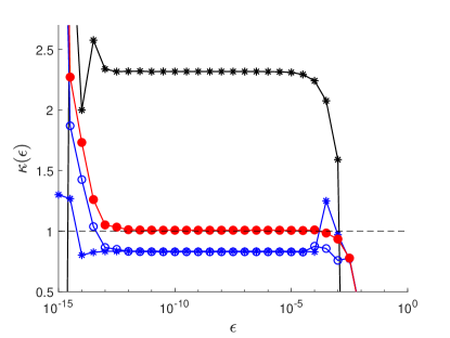
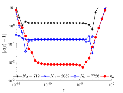
Figure 3: The behavior of (a) $\kappa(\epsilon)$ and (b) $\log_{10}\lvert\kappa(\epsilon)-1\rvert$ as functions of $\epsilon$ while checking the consistency of used gradients computed for model #1. In both graphs, red circles show results for $\kappa_{\alpha}(\epsilon)$ and $N_{\Omega}=7,726$, while the rest relates to the application of the $\kappa$-test to both controls $\alpha$ and $\mathcal{P}$ in domain $\Omega$ with different spatial discretizations.

Figure 3(a) demonstrates such behavior over a range of $\epsilon$ spanning about 10 orders of magnitude for $\bm{\nabla}_{\alpha}\mathcal{J}$ (in red) discretized in the same manner as domain $\Omega$, e.g., with $N_{\Omega}=7,726$. As can be expected, the quantity $\kappa(\epsilon)$ deviates from the unity for very small values of $\epsilon$ due to the subtractive cancelation (round–off) errors and also for large values of $\epsilon$ due to the truncation errors (both of which are well–known effects). In addition, the quantity $\log_{10}\lvert\kappa(\epsilon)-1\rvert$ plotted in Figure 3(b) shows how many significant digits of accuracy are captured in a given gradient evaluation.

Similarly, we apply the same $\kappa$-test to check the correctness of all steps involved in gradient computations associated with control $\mathcal{P}$, as given by (22) with (23) and (17). However, as discussed in Section 3.3, computing $\bm{\nabla}_{\mathcal{P}}\mathcal{J}$ involves FD estimations of $\bm{\nabla}_{\mathcal{P}}\sigma$ whose accuracy depends on the choice of perturbations $\Delta\mathcal{P}_{i}$. Figure 4(a) shows the obtained results after applying the $\kappa$-test when $\Delta\mathcal{P}_{i}$ are constant vectors with all components equal to $\delta\mathcal{P}$ ranging between $10^{-4}$ and $10^{-1}$. The expected “unity plateau” forms, confirming the correctness of all computations; however, its length is limited to about two orders of $\epsilon$ ($10^{-3}\div 10^{-1}$) values. In the same fashion, Figure 4(b) depicts significant digits of accuracy. We use the results of this test to “calibrate” our computational framework by setting $\delta\mathcal{P}$ to $10^{-3}$ for all experiments.

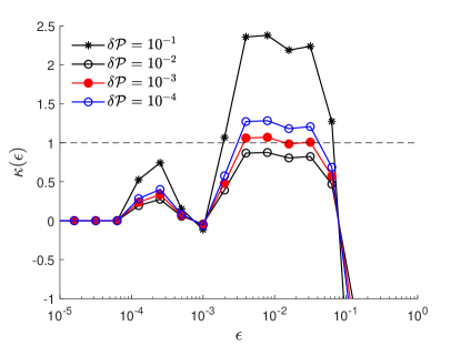
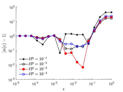
Figure 4: The behavior of (a) $\kappa_{\mathcal{P}}=\kappa(\epsilon)$ and (b) $\log_{10}\lvert\kappa(\epsilon)-1\rvert$ as functions of $\epsilon$ while checking the consistency of gradients $\bm{\nabla}_{\mathcal{P}}\mathcal{J}$ computed for model #1 with different values of parameter $\delta\mathcal{P}$.

Finally, we explore the results obtained by applying the $\kappa$-test to both controls (simultaneously to $\alpha$ and $\mathcal{P}$) to determine a proper discretization of domain $\Omega$ as an obviously better approximation of continuous gradients by finer spatial discretizations here is affected by the added FD approximations in $\bm{\nabla}_{\mathcal{P}}\mathcal{J}$ parts. Although the results provided in Figures 3(a) and 3(b) do not show a significant difference in using $N_{\Omega}=2,032$ and $N_{\Omega}=7,726$, we will use the latter as the number of FEM elements for all numerical experiments and all models in this paper to ensure better resolution for the reconstructed images.

4.2.2 Model #1: Validating Performance

In this section, we will prove the superior performance of the proposed computational framework supplied with the fine-scale gradient-based and coarse-scale binary tuning optimization algorithms, as detailed in Section 3. First, we refer to Figure 5; it shows the results of applying this methodology to our model #1 and a comparison of the computational performance observed while employing different optimizers, namely

• gradient-based sequential quadratic, nonlinear interior point, and sequential convex programming algorithms by respectively SNOPT [20], IPOPT [30], and MMA [27],

• previously used in [7, 6] derivative-free CD method customized to a predefined order of controls.

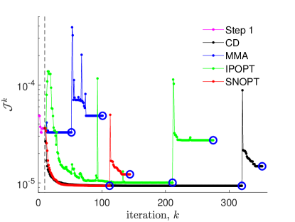
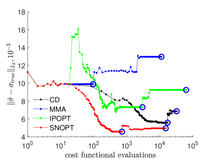
Figure 5: Optimization results for model #1: (a) cost functionals $\mathcal{J}^{k}$ as functions of iteration count $k$ and (b) solution errors $\|\sigma^{k}-\sigma_{true}\|_{L_{2}}$ as functions of a number of cost functional evaluations evaluated while employing different optimizers (CD, MMA, IPOPT, and SNOPT). Pink dots in (a) represent Step 1 solutions ($k=1,2,\ldots,10$), and empty blue circles in (a) and (b) show solutions obtained after Step 2 and 3 phases are complete.

Figure 5(a) clearly distinguishes gradient-based SNOPT from other methods by the best results provided by the cost functional $\mathcal{J}^{k}$ evaluated after all optimization stages (including fine-scale optimization and binary tuning at the coarse scale) are complete. We expected a comparable quality of the reconstructed images obtained by SNOPT and CD methods as they use the same core concept of utilizing sample solutions with customized geometry. On top of that, our new approach uses multiscale control space reduction for binary tuning, also paired with gradient-based techniques. It makes the gradient-based implementation (by SNOPT) more advantageous in both the accuracy of the final solutions and the computational speed, as demonstrated in Figure 5(b), by comparing solution errors $\|\hat{\sigma}-\sigma_{true}\|_{L_{2}}$ as functions of a total number of cost functional evaluations (including cases of evaluating cost functionals $\mathcal{J}$ to complete computations for constructing gradients, choosing optimal step size in the gradient-based methods, etc.). We see this measure to examine the overall performance of various approaches to be reasonable, as cost functional evaluations paired with numerical solutions for forward EIT problem (3) contribute to the major part of the computational load (all other parts, in fact, take fractions of a second of the CPU time to be completed).

We are particularly interested in the approach that allows fast and accurate fine-scale images at Step 2 and also accurate coarse-scale binary images to be of comparable quality after applying the Step 3 tuning procedure. The sequential quadratic optimizer SNOPT proves its superior suitability for this task while competing with its predecessor (CD) and other methods that use the same gradients. Figures 6(a-h) provide the results obtained by all used methods on both fine and coarse scales. Figure 6(g) confirms an almost ideal reconstruction of big spots (both for color and shape) and rather satisfactory (due to the size comparable with the size of the applied boundary electrodes) quality of the smallest spot image. Figure 6(i) contributes to this conclusion by comparing the reconstructed values of $\hat{\sigma}_{high}$ that are much closer to the “known” value $\sigma_{c}=0.4$ in the case of gradient-based SNOPT. Finally, we reiterate and conclude on the reasons for the improved computational speed (1,666 vs. 18,112 cost functional evaluations for SNOPT and CD, respectively). Evidently, gradient-based methods are faster as they change all (or, at least, many) controls while CD works only with one control at a time. In addition to this, as seen in Figures 6(j) and 6(k), CD spends some time “re-ranking” all $N_{s}$ samples used to update the reconstructed image by changing their weights $\alpha_{i}$. On the other hand, based on the sensitivity provided in $\bm{\nabla}_{\alpha}\mathcal{J}$, SNOPT sets the “ranks” at the beginning of Step 2 and focuses on their qualities afterward.

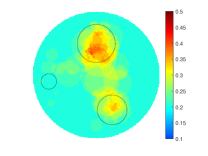
(a) MMA

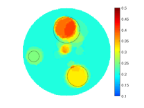
(b) IPOPT

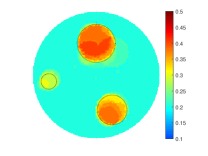
(c) SNOPT

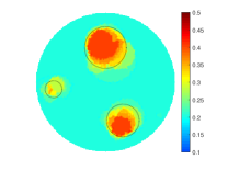
(d) CD

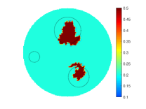
(e) MMA

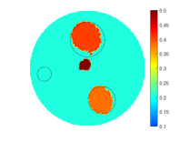
(f) IPOPT

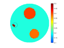
(g) SNOPT

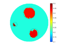
(h) CD

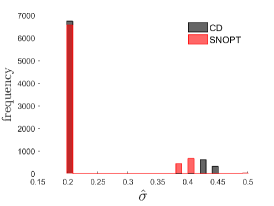
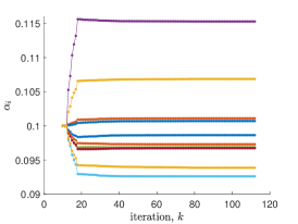
(i) SNOPT

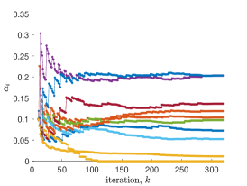
(j) CD

Figure 6: Model #1. (a-h) Solution images obtained by (a,e) MMA, (b,f) IPOPT, (c,g) SNOPT, and (d,h) CD after completing (a-d) Step 2 and (e-h) Step 3. (i) Histograms for solutions obtained by (black) CD and (red) SNOPT. The dashed circles are added to represent the location of cancer-affected regions taken from known $\sigma_{true}(x)$ in Figure 1(a). (j,k) History of changes in weights $\alpha_{i}$ when applying (j) SNOPT and (k) CD methods.

4.3 Validation on Complicated Models

Based on the results obtained for our model #1 and described in the previous section, we conclude on the superior performance brought to the proposed computational framework by employing a multiscale gradient-based search and control space reduction for binary tuning. As shown by practical experiments, the efficacy of the former is subject to a particular optimizer, and the suitability of the latter appears questionable for more complicated models. Therefore, in this section, we discuss the results obtained using this new framework now applied to models with a significantly increased level of complexity to explore any bounds for its applicability. So far, the new algorithm confirms its ability to accurately reconstruct circular-shaped cancerous regions of various sizes at multiple locations. Here, the added complications are non-circular shapes for those regions and their varied conductivities $\sigma_{c}$. The rest of our computational results will compare the performance of the SNOPT and CD optimizers based on data with 0.5% noise.

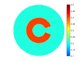
(a) model #2

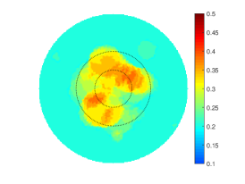
(b) SNOPT: Step 2

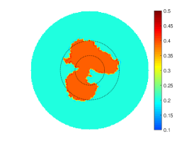
(c) SNOPT: Step 3

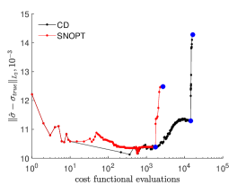
(d) solution error

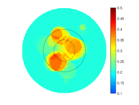
(e) CD: Step 2

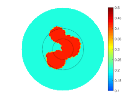
(f) CD: Step 3

Figure 7: (a) EIT model #2: true electrical conductivity $\sigma_{true}(x)$. (b,c,e,f) Solution images obtained by (b,c) SNOPT and (e,f) CD after completing (b,e) Step 2 and (c,f) Step 3. The dashed circles are added to represent the C-shape of the cancer-affected region taken from known $\sigma_{true}(x)$ in (a). (d) Solution errors $\|\sigma^{k}-\sigma_{true}\|_{L_{2}}$ as functions of a number of cost functional evaluations evaluated while employing (black) CD and (red) SNOPT optimizers. Blue dots represent solutions obtained after Step 2 and 3 phases are complete.

We create our next model (#2) to check the method’s performance when cancer-affected areas depart from circular shapes, e.g., as the one in Figure 7(a), showing an image with a C-shape region. Although using the same collection $\mathcal{C}(10,0000)$ of samples containing only circles of various radii does not assume such shapes, the reconstructions obtained by both SNOPT and CD seem acceptable; see Figures 7(c) and 7(f), respectively. Similar to model #1, gradient-based SNOPT shows significantly better performance for quality and computational speed at both Step 2 and 3 optimization phases; refer to Figure 7(d) showing the solution error and blue dots representing solutions obtained after both phases are complete. Images obtained after Step 2, in Figures 7(b) and 7(e), confirm the superior performance added by using gradients improved by the Step 3 tuning procedure that indicates its suitability for such shapes. As explored in [7, 6], this performance may be further enhanced, even in the presence of noise, once we increase the maximum number of circles $N_{c,max}$ in the samples. It proves the potential of the proposed methodology in applications with models bearing rather complex geometry.

To further experiment with the applicability and performance of various parts in the proposed computational algorithm, we modified our model #1 by changing the electrical conductivity (high values) inside the cancerous spots while keeping the same their mutual positioning and sizes. Figure 8(a) displays model #1 after this modification (model #3), where we set $\sigma_{c}$ to 0.3, 0.4, and 0.35 for the big, medium-size, and small spots, respectively.

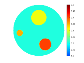
(a) model #3

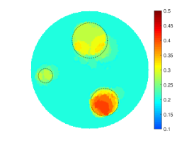
(b) SNOPT: Step 2

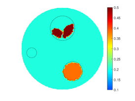
(c) SNOPT: Step 3

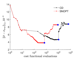
(d) solution error

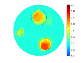
(e) CD: Step 2

(f) CD: Step 3

Figure 8: (a) EIT model #3: true electrical conductivity $\sigma_{true}(x)$. (b,c,e,f) Solution images obtained by (b,c) SNOPT and (e,f) CD after completing (b,e) Step 2 and (c,f) Step 3. The dashed circles are added to represent the location of cancer-affected regions taken from known $\sigma_{true}(x)$ in (a). (d) Solution errors $\|\sigma^{k}-\sigma_{true}\|_{L_{2}}$ as functions of a number of cost functional evaluations evaluated while employing (black) CD and (red) SNOPT optimizers. Blue dots represent solutions obtained after Step 2 and 3 phases are complete.

The visual analysis of the fine-scale solutions obtained using gradient-based (SNOPT) and derivative-free (CD) searches after completing Step 2 reveals good results in recovering the positions of all three spots and reconstructing their shapes for both methods; refer to Figures 8(b) and 8(e), respectively. As previously, SNOPT supplied by gradient information performs better for quality (better match for colors, especially for the two big spots) and computational speed (683 vs. 10,138 cost functional evaluations to complete Step 2), confirmed by the analysis of the solution error provided in Figure 8(d). It concludes with the applicability of the proposed methodology to differentiate between cancerous spots with varied conductivities even though the used samples are “unaware” of that, making this methodology less dependent on the prior knowledge of the simulated phenomena. The same analysis applied to the results for binary tuning during Step 3, Figures 8(c) and 8(f), concludes on the lower quality of obtained images for both methods. We explain it by the presence of noise (0.5%) in the supplied data – the known effect reported earlier – procedure in Step 2 has less sensitivity to noise [7, 6] than binary tuning in Step 3 [17]. Although the overall outcomes are rather satisfactory and promising, it leaves space for further development for the binary tuning phase and better “communication” between computational components while transitioning from Step 2 to Step 3.

4.4 Applications to Cancer Detection

In the last part of our numerical experiments with the proposed optimization framework, our particular interest is in applying it to cases seen in the medical practice during cancer-related screening procedures. We utilize our last two models (#4 and #5) based on the mammogram (X-ray) and magnetic resonance (MRI) images, respectively, of real breast cancer cases available in [8, 32]; refer to [17] for the details on creating these models by converting the actual images to their binary versions and obtaining synthetic data in place of the true measurements. Model #4 shows an invasive ductal carcinoma with an irregular shape and spiculated margins; see Figure 9(a). Our final model (#5) refers to even more complicated cases seen in the medical practice when multiple regions suspected of being cancerous are present and characterized by different sizes and nontrivial shapes; see Figure 10(a). This model shows multiple (three) spots also identified as invasive ductal carcinoma with irregular shapes and spiculated margins.

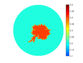
(a) model #4

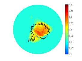
(b) SNOPT: Step 2

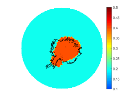
(c) SNOPT: Step 3

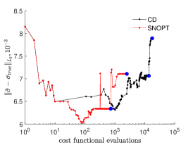
(d) solution error

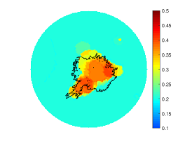
(e) CD: Step 2

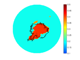
(f) CD: Step 3

Figure 9: (a) EIT model #4: true electrical conductivity $\sigma_{true}(x)$. (b,c,e,f) Solution images obtained by (b,c) SNOPT and (e,f) CD after completing (b,e) Step 2 and (c,f) Step 3. The black dots are added to represent the location of the cancer-affected region taken from known $\sigma_{true}(x)$ in (a). (d) Solution errors $\|\sigma^{k}-\sigma_{true}\|_{L_{2}}$ as functions of a number of cost functional evaluations evaluated while employing (black) CD and (red) SNOPT optimizers. Blue dots represent solutions obtained after Step 2 and 3 phases are complete.

Figures 9(b) and 9(e) demonstrate the images obtained while running fine-scale optimization driven by gradient-based SNOPT and derivative-free CD optimizers, respectively. Although the solution to the inverse EIT problem of model #4 is very challenging due to the nontrivial shape of the cancerous spot at the center, the quality of both images is rather good and further significantly improved after applying binary tuning in Step 3; refer to Figures 9(c) and 9(f). Here, consistent with the previous results, SNOPT conducts the reconstruction better in quality (better match for both color and shape) and computational speed (995 vs. 14,099 cost functional evaluations to complete both Steps 2 and 3), confirmed by the analysis based on the solution error; see Figure 9(d). The results obtained here by gradient-based SNOPT are apparently of much higher quality than those reported in [17] obtained by gradient- and PCA-based multiscale optimization paired with the added regularization.

Finally, we refer to the results obtained for the most complicated case by model #5. Figures 10(b,c) and 10(e,f) present the images produced by SNOPT and CD optimizers, respectively. We admit the same level of accuracy in reconstructing two spots and the biggest one after Steps 2 and 3, respectively, by both optimizers. Figure 10(d), showing the solution error, also confirms more or less the same performance for both. This model indeed sets the limits for the current implementation of the proposed computational framework due to the nontrivial shapes of the cancerous spots and their small sizes. Although the overall performance is fairly modest, the final results here are of much better quality than reported previously in [17], where extra data was added through applied regularization. It makes the application of our computational framework very promising, having enough space for future developments in both quality of the reconstructed images related to very complex medical cases and computational efficacy sought to help implement the approach for use in the medical practice.

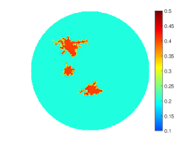
(a) model #5

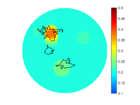
(b) SNOPT: Step 2

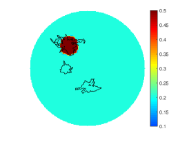
(c) SNOPT: Step 3

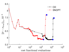
(d) solution error

(e) CD: Step 2

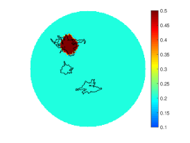
(f) CD: Step 3

Figure 10: (a) EIT model #5: true electrical conductivity $\sigma_{true}(x)$. (b,c,e,f) Solution images obtained by (b,c) SNOPT and (e,f) CD after completing (b,e) Step 2 and (c,f) Step 3. The black dots are added to represent the locations of cancer-affected regions taken from known $\sigma_{true}(x)$ in (a). (d) Solution errors $\|\sigma^{k}-\sigma_{true}\|_{L_{2}}$ as functions of a number of cost functional evaluations evaluated while employing (black) CD and (red) SNOPT optimizers. Blue dots represent solutions obtained after Step 2 and 3 phases are complete.

5 Concluding Remarks

In this work, we developed and validated a highly efficient computational framework for reconstructing images of near-binary types related to physical properties of various models used in biomedical applications, e.g., to assist with the recognition of cancer-affected regions while solving an inverse problem of cancer detection using the electrical impedance tomography technique. In particular, we explored the possibility of applying the proposed solution methodology to the IPCD problems to detect cancerous regions surrounded by healthy tissues, which also have small sizes and boundaries of irregular shapes that appeared to be vital for early cancer detection and easy control of the dynamics of cancer development or treatment progress. We also prove its suitability for models of various complexity seen in diverse applications for biomedical sciences, physics, geology, chemistry, etc. The efficiency of the new approach in both computational speed and accuracy is achieved by combining the advantages of recently developed optimization methods that use sample solutions with customized geometry and multiscale control space reduction, all paired with gradient-based techniques. A practical implementation of this approach has an easy-to-follow design tuned by a nominal number of parameters to govern the entire suite of computational and optimization facilities. We conclude on the high potential of the proposed computational methodology to minimize possibilities for false positive and false negative screening and improve the overall quality of EIT-based procedures.

Despite the superior performance of the proposed framework, there are many ways this optimization algorithm can be tested and further extended, e.g., by applying advanced minimization techniques to perform local and global searches, using adaptive schemes for a smooth transition of the obtained solutions between computational phases, flexible (efficient) termination criteria, and different metrics to evaluate the quality of the overall reconstruction. We plan further research on the measurement structure, e.g., considering 32-electrode schemes in 2D, shifting to 3D models, and improving sensitivity by optimizing the configuration of available data. We also expect to have more benefits for saving computational time from applying parallelization to the entire computational framework, including solving forward EIT problems. Finally, we are interested in other expansions leading to reliable and accurate results for near-real cases by using bimodal distributions and fully anisotropic models.

Acknowledgements

We wish to thank the anonymous reviewers for their valuable comments and suggestions to improve the clarity of the presented approach and the overall readability of this paper.

References

- [1] Abascal, J.F.P.J., Lionheart, W.R.B., Arridge, S.R., Schweiger, M., Atkinson, D., Holder, D.S.: Electrical impedance tomography in anisotropic media with known eigenvectors. Inverse Problems 27(6), 1–17 (2011)
- [2] Abdulla, U.G., Bukshtynov, V., Seif, S.: Cancer detection through electrical impedance tomography and optimal control theory: Theoretical and computational analysis. Mathematical Biosciences and Engineering 18(4), 4834–4859 (2021)
- [3] Adler, A., Arnold, J., Bayford, R., Borsic, A., Brown, B., Dixon, P., Faes, T.J., Frerichs, I., Gagnon, H., Gärber, Y., Grychtol, B., Hahn, G., Lionheart, W., Malik, A., Stocks, J., Tizzard, A., Weiler, N., Wolf, G.: GREIT: towards a consensus EIT algorithm for lung images. In: 9th EIT conference 2008, 16-18 June 2008, Dartmouth, New Hampshire. CiteSeerX, Pennsylvania State University (2008)
- [4] Adler, A., Gaburro, R., Lionheart, W.: Handbook of Mathematical Methods in Imaging, chap. Electrical Impedance Tomography, pp. 701–762. Springer New York, New York, NY (2015)
- [5] Adler, A., Holder, D.: Electrical Impedance Tomography. Methods, History, and Applications, 2nd edn. CRC Press, Boca Raton, FL (2022)
- [6] Arbic II, P.R.: Optimization Framework for Reconstructing Biomedical Images by Efficient Sample-based Parameterization. M.S. Thesis, Florida Institute of Technology, Scholarship Repository (2020). URL http://hdl.handle.net/11141/3220
- [7] Arbic II, P.R., Bukshtynov, V.: On reconstruction of binary images by efficient sample-based parameterization in applications for electrical impedance tomography. International Journal of Computer Mathematics 99(11), 2272–2289 (2022)
- [8] Bassett, L.W., Conner, K., IV, M.: The abnormal mammogram. In: Holland-Frei Cancer Medicine (2003)
- [9] Bera, T.K.: Applications of electrical impedance tomography (EIT): A short review. IOP Conference Series: Materials Science and Engineering 331, 012,004 (2018)
- [10] Borcea, L.: Electrical impedance tomography. Inverse Problems 18, 99–136 (2002)
- [11] Brown, B.: Electrical impedance tomography (EIT): A review. Journal of Medical Engineering and Technology 27(3), 97–108 (2003)
- [12] Bukshtynov, V.: Computational Optimization: Success in Practice. Chapman and Hall/CRC (2023). URL https://www.routledge.com/Computational-Optimization/Bukshtyn%ov/p/book/9781032229478
- [13] Bukshtynov, V., Protas, B.: Optimal reconstruction of material properties in complex multiphysics phenomena. Journal of Computational Physics 242, 889–914 (2013)
- [14] Bukshtynov, V., Volkov, O., Protas, B.: On optimal reconstruction of constitutive relations. Physica D: Nonlinear Phenomena 240(16), 1228–1244 (2011)
- [15] Calderon, A.P.: On an inverse boundary value problem. In: Seminar on Numerical Analysis and Its Applications to Continuum Physics, pp. 65–73. Soc. Brasileira de Mathematica, Rio de Janeiro (1980)
- [16] Cheney, M., Isaacson, D., Newell, J.: Electrical impedance tomography. SIAM Review 41(1), 85–101 (1999)
- [17] Chun, M.M., Edwards, B.L., Bukshtynov, V.: Multiscale optimization via enhanced multilevel PCA-based control space reduction for electrical impedance tomography imaging. Computers and Mathematics with Applications 157, 215–234 (2024)
- [18] Chun, M.M.F.M.: Multiscale Optimization via Multilevel PCA-based Control Space Reduction in Applications to Electrical Impedance Tomography. M.S. Thesis, Florida Institute of Technology, Scholarship Repository (2022). URL http://hdl.handle.net/11141/3558
- [19] Davis, T.A.: Algorithm 832: UMFPACK V4.3 – an unsymmetric-pattern multifrontal method. ACM Transactions on Mathematical Software (TOMS) 30(2), 196–199 (2004)
- [20] Gill, P., Murray, W., Saunders, M.: User’s Guide for SNOPT Version 7: Software for Large-Scale Nonlinear Programming. Stanford University, Stanford, CA (2008)
- [21] Hadamard, J.: Lectures on the Cauchy Problem in Linear Partial Differential Equations. Yale University Press, New Haven, CT (1923)
- [22] Hecht, F.: New development in FreeFem++. Journal of Numerical Mathematics 20(3-4), 251–265 (2012)
- [23] Koolman, P.M., Bukshtynov, V.: A multiscale optimization framework for reconstructing binary images using multilevel PCA-based control space reduction. Biomedical Physics & Engineering Express 7(2), 025,005 (2021)
- [24] Krogstad, S., Nilsen, H.: Efficient adjoint-based well-placement optimization using flow diagnostics proxies. Computational Geosciences 26, 883–896 (2022)
- [25] Lionheart, W.: EIT reconstruction algorithms: Pitfalls, challenges and recent developments. Physiological Measurement 25(1), 125–142 (2004)
- [26] Somersalo, E., Cheney, M., Isaacson, D.: Existence and uniqueness for electrode models for electric current computed tomography. SIAM Journal on Applied Mathematics 52(4), 1023–1040 (1992)
- [27] Svanberg, K.: The method of moving asymptotes — a new method for structural optimization. International Journal for Numerical Methods in Engineering 24(2), 359–373 (1987)
- [28] Uhlmann, G.: Electrical impedance tomography and Calderón’s problem. Inverse Problems 25(12), 123,011 (2009)
- [29] Volkov, O., Bellout, M.: Gradient-based constrained well placement optimization. Journal of Petroleum Science and Engineering 171, 1052–1066 (2018)
- [30] Wachter, A., Kawajir, Y.: Introduction to Ipopt: A tutorial for downloading, installing, and using Ipopt. COIN-OR, IBM Research (2010)
- [31] Wang, Z., Yue, S., Wang, H., Yanqiu: Data preprocessing methods for electrical impedance tomography: a review. Physiological Measurement 41(9), 09TR02 (2020)
- [32] Weinstein, S.P.: Evolving role of MRI in breast cancer imaging. PET Clinics 4(3), 241–253 (2009)
- [33] Zou, Y., Guo, Z.: A review of electrical impedance techniques for breast cancer detection. Medical Engineering and Physics 25(2), 79–90 (2003)