Bayesian neural networks via MCMC: a Python-based tutorial

Abstract

Bayesian inference provides a methodology for parameter estimation and uncertainty quantification in machine learning and deep learning methods. Variational inference and Markov Chain Monte-Carlo (MCMC) sampling techniques are used to implement Bayesian inference. In the past three decades, MCMC methods have faced a number of challenges in being adapted to larger models (such as in deep learning) and big data problems. Advanced proposals that incorporate gradients, such as a Langevin proposal distribution, provide a means to address some of the limitations of MCMC sampling for Bayesian neural networks. Furthermore, MCMC methods have typically been constrained to use by statisticians and are still not prominent among deep learning researchers. We present a tutorial for MCMC methods that covers simple Bayesian linear and logistic models, and Bayesian neural networks. The aim of this tutorial is to bridge the gap between theory and implementation via coding, given a general sparsity of libraries and tutorials to this end. This tutorial provides code in Python with data and instructions that enable their use and extension. We provide results for some benchmark problems showing the strengths and weaknesses of implementing the respective Bayesian models via MCMC. We highlight the challenges in sampling multi-modal posterior distributions in particular for the case of Bayesian neural networks, and the need for further improvement of convergence diagnosis.

1 Introduction

Bayesian inference provides a probabilistic approach for parameter estimation in a wide range of models used across the fields of machine learning, econometrics, environmental and Earth sciences [1, 2, 3, 1, 4, 5]. The term ’probabilistic’ refers to representation of unknown parameters as probability distributions rather than using fixed point estimates as in conventional optimisation methods and machine learning models where gradient-based methods are prominent [6]. The probability representation of unknown parameters requires a different approach to optimisation and, from the machine learning and computational statistics point-of-view, this is known as sampling.

Markov Chain Monte-Carlo (MCMC) sampling methods have been prominent for inference (estimation) of model parameters via the posterior distribution (probability distribution). In other words, Bayesian methods attempt to quantify the uncertainty in model parameters by marginalising over the predictive posterior distribution. Hence, in the case of neural networks, MCMC methods can be used to implement Bayesian neural networks that represent weights and biases as probability distributions [7, 8, 9, 10, 11, 7]. Probabilistic machine learning provides natural way of providing uncertainty quantification in predictions [12] since the uncertainties can be obtained by probabilistic representation of parameters. This inference procedure can be seen as a form of learning (optimisation) applied to the model parameters [8]. In this tutorial, we employ linear models and simple neural networks to demonstrate the use of MCMC sampling methods. The probabilistic representation of weights and biases in the respective models allows uncertainty quantification on model predictions.

We note that MCMC refers to a family of algorithms for implementing Bayesian inference for parameter and uncertainty estimation in models. The range of models to which Bayesian inference is applied, including statistical, graphical, and machine learning models; has led to the existence of a wide range of MCMC sampling algorithms. Some of the prominent ones are Metropolis Hastings algorithm [13, 14, 15], Gibbs sampling [16, 17, 18], Langevin MCMC [19, 20, 21], rejection sampling [22, 23], sequential MCMC [24], adaptive MCMC [25], parallel tempering (tempered) MCMC [26, 27, 28, 29], reversible-jump MCMC [30, 31], specialised MCMC methods for discrete time series models[32, 33, 34], constrained parameter and model settings [35, 36], and likelihood free MCMC [37]. MCMC sampling methods have also been used for data augmentation [38, 39], model fusion [40], model selection [41, 42], and interpolation [43]. Apart from this, we note that MCMC methods have been prominent in a wide range of applications that include geophysical inversions [44, 45, 46], geo-scientific models [5, 47, 48], environmental and hydrological modelling [49, 50], bio-systems modelling [51, 52, 53], and quantitative genetics [54, 55].

In the case of Bayesian neural networks, the large number of model parameters that emerge from large neural network architectures and deep learning models pose challenges for MCMC sampling methods. Hence, progress in the application of Bayesian approaches to big data and deep neural networks has been slow. Research in this space has included a number of methods that have been fused with MCMC such as gradient-based methods [56, 21, 57, 58, 59], and evolutionary (meta-heuristic) algorithms which include differential evolution, genetic algorithms, and particle swarm optimisation [60, 61, 62, 63].

This use of gradients in MCMC was initially known as Metropolis-adjusted Langevin dynamics [21] and has shown promising performance for linear models [58] and has also been extended to Bayesian neural networks [59]. Another direction has been the use of better exploration features in MCMC sampling such as parallel tempering MCMC with Langevin-gradients and parallel computing [59], providing a competitive alternative to stochastic gradient-descent [64] and Adam optimizers [6] with the addition of uncertainty quantification in predictions. These methods have also been applied to Bayesian deep learning models such as Bayesian autoencoders [65] and Bayesian graph convolutional neural networks (CNNs) [66] which require millions of trainable parameters to be represent as posterior distributions. Recently, Kapoor et al. [63] combined tempered MCMC with particle swarm optimisation-based proposal distribution in an parallel computing environment and showed that the hybrid approach samples posterior distribution more effectively when compared with the conventional approach.

Hamiltonian Monte Carlo (HMC) approach that uses gradient-based proposal distributions [57] and has been effectively applied to Bayesian neural networks [67]. In similar way, Langevin dynamics can be used to incorporate gradient-based stepping with Gaussian noise into the proposal distribution [58]. HMC avoids random walk behaviour using an auxiliary momentum vector and implementing Hamiltonian dynamics where the momentum samples are discarded after later. The samples are hence less correlated and tend converge to the target distribution more rapidly.

Variational inference (VI) provides an alternative approach to MCMC methods to approximate Bayesian posterior distribution [68, 69]. Bayes by backpropagation is a VI method that showed competitive results when compared to stochastic gradient descent and dropout methods used as approximate Bayesian methods [70]. Dropout is a regularisation technique that is relatively simple to implement and involves randomly dropping selected weights in forward-pass operation of backpropagation. This improves the generalization performance of neural networks and has been widely adopted [71]. Gal and Ghahramani [72] presented an approximate Bayesian methodology based on dropout-based regularisation which has been used for other deep learning models such as CNNs [73]. Later, Gal and Ghahramani [74] presented VI-based dropout technique for recurrent neural networks (RNNs); particularly, long-short term memory (LSTM) and gated recurrent unit (GRU) models for language modelling and sentiment analysis tasks.

We argue that the use of dropouts used for regularisation cannot be seen as a an alternative of MCMC sampling directly from the posterior distribution. In this case, we do not know the priors nor know much about the posterior distribution and there is little theoretical rigour, only computational efficacy or capturing noise and uncertainty during model training. Furthermore, in the Bayesian methodology, a probabilistic representation using priors is needed which is questionable in the dropout methodology for Bayesian computation. Given that VI methods are seen as approximate Bayesian methods, we need to invest more effort in directly sampling from the posterior distribution in case of Bayesian deep learning models. This can only be possible if both communities (i.e., statistics and machine learning) are aware about the strengths and weaknesses of MCMC methods for sampling Bayesian neural networks that span hundreds to thousands of parameters, and go orders of magnitude higher when looking at Bayesian deep learning models. The progress of MCMC for deep learning has been slow due to lack of implementation details, libraries and tutorials that provide that balance of theory and implementation.

In this paper, we present a Python-based tutorial for MCMC methods that covers simple Bayesian linear models and Bayesian neural networks. We provide code in Python with data and instructions that enable their use and extension. We provide results for some benchmark problems showing the strengths and weaknesses of implementing the respective Bayesian models via MCMC with detailed instructions for every code sample in a related Github repository so that it is easy to clone and run. Our tutorial is simple, and relies on basic Python libraries such as numpy. We do not use advanced libraries as the goal is to serve as a go-to document for beginners who have basic knowledge of machine learning models, and need to get hands on experience with MCMC sampling. Hence, this is a code-based computational tutorial with theoretical background. Finally, we highlight the challenges in sampling multi-modal posterior distributions in the case of Bayesian neural networks and shed light on the use of convergence diagnostics.

The rest of the paper is organised as follows. In Section 2, we present a background and literature review of related methods. Section 3 presents the proposed methodology, followed by experiments and results in Section 4. Section 5 provides a discussion and Section 6 concludes the paper with directions of future work.

2 Background

2.1 Bayesian inference

We recall that Bayesian methods account for the uncertainty in prediction and decision making via the posterior distribution [75]. Note that the posterior is the conditional probability determined after taking into account the prior distribution and the relevant evidence or data via sampling methods. Thomas Bayes (1702 – 1761) presented and proved a special case of the Bayes’ theorem [76, 77] which is the foundation of Bayesian inference. However, it was Pierre-Simon Laplace (1749 – 1827) who introduced a general version of the theorem and used it to approach problems [78]. Figure 1 gives an overview of the Bayesian inference framework that uses data with a prior and likelihood to construct to sample from the posterior distribution. This is the building block of the rest of the lessons that will feature Bayesian logistic regression and Bayesian neural networks.

Bayesian inference estimates unknown parameters using prior information or belief about the variable. Prior information is captured in the form of a distribution. A simple example of a prior belief is a distribution that has a positive real-valued number in some range. This essentially would imply a belief that our result or posterior distribution would likely be a distribution of positive numbers in some range which would be similar to the prior but not the same. If the posterior and prior both follow the same type of distribution, this is known as a conjugate prior [79]. If the prior provides useful information about the variable, rather than very loose constraints, it is known as informative prior. The prior distribution is based on expert knowledge (opinion) and is also dependent on the domain for different types of models [80, 81].

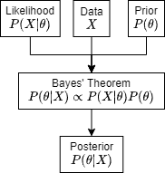
Figure 1: The relationship of the likelihood with data and prior distribution is shown for sampling the posterior distribution.

The need for efficient sampling methods to implement Bayesian inference has been a significant focus of research in computational statistics. This is especially true in the case of multi-modal and irregular posterior distributions [82, 83, 29] which tend to dominate in Bayesian neural network problems [10, 84]. MCMC sampling methods are used to update the probability for a hypothesis (proposal $\Theta$) as more information becomes available. The hypothesis is given by a prior probability distribution that expresses one’s belief about a quantity (or free parameter in a model) before some data ($\bf{d}$) are observed. MCMC methods use sampling to construct the posterior distribution ($P(\Theta|\bf{x})$), iteratively using a proposal distribution, prior distribution $P(\Theta)$, and likelihood function.

$$P(\Theta|\bf{x})=\frac{P(\bf{d}|\Theta)\times P(\Theta)}{P(d)}$$ (1)

We note that $P(\bf{d}|\Theta)$ could be seen as the likelihood distribution in disguise. $P(\bf{d})$ is the marginal distribution of the data and is often seen as a normalising constant and ignored. Hence, ignoring it, we can also express the above in this way

$$P(\Theta|\bf{x})\propto P(\bf{x}|\Theta)\times P(\bf{\Theta})$$ (2)

The likelihood function is a function of the parameters of a given model provided specific observed data [85]. The likelihood function can be seen as a measure of fit to the data for the proposals which are drawn from the proposal distribution. Hence, from an optimisation perspective, the likelihood function can be seen as a fitness or error function. The posterior distribution is constructed after taking into account the relevant evidence (data) and prior distribution, with the likelihood that considers the proposal and the model. MCMC methods essentially implement Bayesian inference via a numerical approach that marginalizes or integrates over the posterior distribution [86]. Note that probability and likelihood are not the same in the field of statistics, while in everyday language they are used as if they are the same. The term ”probability” refers to the possibility of something happening in relation to a given distribution of data. The likelihood refers to the likelihood function that provides a measure of fit in relation to a distribution. The likelihood function indicates which parameter (data) values are more likely than others in relation to a distribution. Further and detailed explanations regarding Bayesian inference and MCMC sampling is given here [87, 88].

2.2 Probability distributions

2.2.1 Gaussian (Normal) Distribution

A normal probability density or distribution, also known as the Gaussian distribution, is described by two parameters, mean ($\mu$) around which the distribution is centered and the standard deviation ($\sigma$) which describes the spread (sometimes described instead by the variance, $\sigma^{2}$). Using these two parameters, we can fit a probability (normal) distribution to data from some source. In similar way, given a probability distribution, we can generate data and this process is known as sampling from the distribution. In sampling the distribution we simply present random data points (uniform) to the distribution and get data that is, in a way, transformed by the distribution. These parameters determine the shape of the probability distribution, e.g., if it is peaked or spread. Note that the normal distribution is symmetrical in nature and caters for negative and positive numbers of real data.

Equation 3 presents the Gaussian distribution probability density function (PDF) for parameters $\mu$ and $\sigma$.

$$f(x)=\frac{1}{\sqrt{2\pi\sigma^{2}}}exp\left({-\frac{1}{2}\left(\frac{x-\mu}{\sigma}\right)^{2}}\right)$$ (3)

We will sample from this distribution in Python via the NumPy library [89] to sample from the various distributions discussed in this tutorial and SciPy library [90] to get a representation of the PDF i.e., the probability distribution. The associated github repository contains the code to generate Figures 2 to 5 using the Seaborn and Matplotlib Python libraries.

⬇

1import numpy as np

2from numpy import random

3from scipy import stats

4

5# 10 random draws from a standard Gaussian distribution - N(0,1)

6samples = random.randn(10)

7# Gaussian distribution PDF with mean of 4 and standard deviation of 0.5

8x = np.linspace(0, 8, 100)

9pdf = stats.norm.pdf(x, loc=4, scale=0.5)

Listing 1: Random number generation for a Gaussian distribution

We note that the mean and standard deviation are purely based on the data and it will change depending on the dataset. Let us visualise what happens when standard deviation changes and mean remains the same for the distribution as shown in Figure 2.

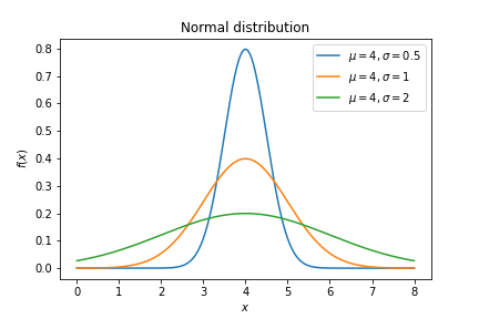
Figure 2: Normal distributions with the same mean and different standard deviations.

We can review some more examples where changes to the mean and standard deviation gives us different shapes of the PDF as shown in Figure 3.

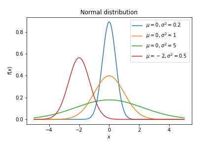
Figure 3: Normal distributions with different parameters, i.e mean and the standard deviation.

2.2.2 Multivariate Normal distribution

The multivariate normal distribution or joint normal distribution generalises univariate normal distribution to more variables or higher dimensions as shown in the PDF in Equation 4.

$$f(x_{1},\ldots,x_{M})=\frac{1}{\sqrt{(2\pi)^{M}|\boldsymbol{\Sigma}|}}\exp\left(-\frac{1}{2}({\mathbf{x}}-{\boldsymbol{\mu}})^{\mathrm{T}}{\boldsymbol{\Sigma}}^{-1}({\mathbf{x}}-{\boldsymbol{\mu}})\right)$$ (4)

where $\mathbf{x}$ is a real $M$-dimensional column vector and $|\Sigma|$ is the determinant of symmetric covariance matrix which is positive definite.

2.2.3 Gamma distribution

A gamma distribution is defined by the parameters shape ($\alpha$) and rate ($\beta$) as shown below.

$$f(x;\alpha,\beta)=\frac{\beta^{\alpha}x^{\alpha-1}e^{-\beta x}}{\Gamma(\alpha)}$$ (5)

for $x>0\quad\alpha,\beta>0$; where $\Gamma(n)=(n-1)!$. Figure 4 presents the Gamma distribution for various parameter combinations, with corresponding Python code given below.

⬇

1# 10 (size) random draws from a Gamma distribution with a shape parameter of 2 and scale (1/rate) of 2

2samples = random.gamma(2,scale=2,size=10)

3# Gamma distribution PDF with a shape parameter of 2 and scale (1/rate) of 2

4x = np.linspace(0, 10, 100)

5pdf = stats.gamma.pdf(x, a=2, scale=2)

6

7# Inverse Gamma distribution PDF with a shape parameter of 2 and scale of 1

8x = np.linspace(0, 5, 100)

9pdf = stats.invgamma.pdf(x, a=2, scale=1)

Listing 2: Random number generation for the Gammma and inverse Gamma distributions

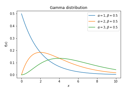
Figure 4: Gamma distributions with different shape and rate parameters ($\alpha$ and $\beta$).

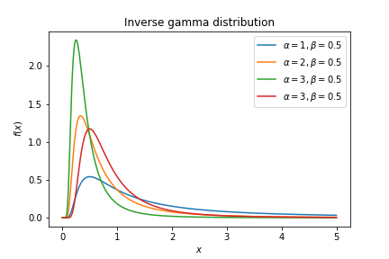
Figure 5: Inverse gamma distributions with different shape and rate parameters ($\alpha$ and $\beta$).

The corresponding inverse-Gamma (IG) distribution takes the same parameters with examples given in Figure 5 and is more appropriate for real positive numbers.

2.2.4 Binomial distribution

So far, we have only addressed real numbers with respective probability distributions; however, we need to also consider discrete numbers. The Bernoulli distribution is a discrete probability distribution typically used for modelling binary classification problems. We begin with an example where a variable $x$ takes the value 1 with probability $p$ and the value 0 with probability $q=1-p$. The probability mass function for this distribution over the possible outcomes ($x$) is given by Equation 6.

$$f(x;p)=p^{x}(1-p)^{1-x}$$ (6)

for $x\in{0,1}$. The probability of getting exactly $k$ successes ($x=1$) in $n$ independent Bernoulli trials ($f(k,n,p)$) is given as $\Pr(k;n,p)$ in Equation 7.

$$\Pr(k;n,p)=\binom{n}{k}p^{k}(1-p)^{n-k}$$ (7)

for $k=0,1,2,...,n$, where $\binom{n}{k}=\frac{n!}{k!(n-k)!}$. Listing 3 below shows the implementation in Python.

⬇

1# 10 (size) random draws from a Binomial distribution with a shape parameter of 2 and scale (1/rate) of 2

2samples = random.gamma(2,scale=2,size=10)

3# Binomial distribution PDF with a shape parameter of 2 and scale (1/rate) of 2

4x = np.linspace(0, 10, 100)

5pdf = stats.gamma.pdf(x, a=2, scale=2)

Listing 3: Random number generation for the Binomial distributions

2.2.5 Multinomial distribution

Previously, we catered for the case of two outcomes; however, we can consider the case of more than two outcomes. Suppose a single trial can result in $k\ (k\geq 2)$ possible outcomes numbered $1,2,\ldots,k$ and let $p_{i}=\mathbb{P}(\text{a single trial results in outcome i})$ $(\sum_{i=1}^{k}p_{i}=1)$. For $n$ independent trials, let $X_{i}$ denote the number of trials resulting in outcome $i$ (then $\sum_{i=1}^{k}X_{i}=n$). Then we say that the distribution of $(X_{1},X_{2},\ldots,X_{k})\sim\text{Multinomial}(n;p_{1},p_{2},\ldots,p_{k})$ and it holds

$$\mathbb{P}(X_{1}=x_{1},X_{2}=x_{2},\ldots,X_{k}=x_{k})=\frac{n!}{x_{1}!x_{2}!\ldots x_{k}!}p_{1}^{x_{1}}p_{2}^{x_{2}}\ldots p_{k}^{x_{k}},\ 0<p_{i}<1,\ \sum_{i=1}^{k}p_{i}=1.$$ (8)

3 MCMC

We begin by noting that a Markov process is uniquely defined by its transition probabilities $P(x^{\prime}|x)$ which defines the probability of transitioning from any given state $x$ to another given state $x^{\prime}$. The Markov process has a unique stationary distribution $\pi(x)$ given the following two conditions are met.

1. There must exist a stationary distribution $\pi$ which solves the detailed balance equations, and therefore requires that each transition $x\to x^{\prime}$ is reversible. This implies that for every pair of states $x,x^{\prime}$, the probability of being in state $x$ and moving to state $x^{\prime}$, must be equal to the probability of being in state $x^{\prime}$ and moving to state $x$; hence, $\pi(x)P(x^{\prime}\mid x)=\pi(x^{\prime})P(x\mid x^{\prime})$.

2. The stationary distribution must be unique which is guaranteed by ergodicity of the Markov process [91, 92, 93]. Ergodicity is guaranteed when every state is aperiodic (i.e., the system does not return to the same state at fixed intervals) and positive recurrent (i.e., the expected number of steps for returning to the same state is finite). An ergodic system is one that mixes well, in other words you get the same result whether you average its values over time or over space.

Given that $\pi(x)$ is chosen to be $P(x)$, the condition of detailed balance becomes $P(x^{\prime}\mid x)P(x)=P(x\mid x^{\prime})P(x^{\prime})$ which is re-written as shown in Equation 9.

$$\frac{P(x^{\prime}\mid x)}{P(x\mid x^{\prime})}=\frac{P(x^{\prime})}{P(x)}$$ (9)

Algorithm 1 presents a basic MCMC sampler with random-walk proposal distribution that runs until a maximum number of samples ($N_{max}$) is reached for training data, $\mathbf{d}$.

Data: Training data, $\mathbf{d}$

Result: $N_{max}$ samples from the posterior distribution

- Initialise $x_{0}$ ;

for $i=1$ until $N_{max}$ do

       1. Propose a value $x^{\prime}|x_{i}\sim q(x_{i})$, where $q(.)$ is the proposal distribution;

       2. Given $x^{\prime}$, execute the model $f(x^{\prime},\mathbf{d})$ to compute the predictions (output $y$) and the likelihood;

       3. Calculate the acceptance probability $\alpha=\min\left(1,\frac{P(x^{\prime})}{P(x_{i})}\frac{q(x_{i}\mid x^{\prime})}{q(x^{\prime}\mid x_{i})}\right)$

       4. Generate a random value from a uniform distribution $u\sim U(0,1)$;

       5. Accept or reject proposed value $x^{\prime}$;

       if $u<\alpha$ then

             accept the sample, $x_{i}=x^{\prime}$

      else

             reject current and retain previous sample, $x_{i}=x_{i-1}$

       end if

      

end for

Algorithm 1 A basic MCMC sampler leveraging the Metropolis-Hastings algorithm

Algorithm 1 proceeds by proposing new values of the parameter $x$ (Step 1) from the selected proposal distribution $q(.)$, in this case a uniform distribution between 0 and 1. Conditional on these proposed values, the model $f(x^{\prime},\mathbf{d})$ computes or predicts an output using proposal x’ and data $\mathbf{d}$ (Step 2). We computer the likelihood using the prediction, and employ a Metropolis-Hasting criterion (Step 3) to determine whether to accept or reject the proposal (Step 5). We compare the acceptance ratio $\alpha$ with $u\sim U(0,1)$, this enforces that the proposal is accepted with probability $\alpha$. If the proposal is accepted, the chain moves to this proposed value. If rejected, the chain stays at the current value. The process is repeated until the convergence criterion is met, which in this case is the maximum number of samples ($N_{max}$) defined by the user.

3.1 Priors

The prior distribution is generally based on belief, expert opinion or other information without viewing the data [8, 94]. Information to construct the prior can be based on past experiments or the posterior distribution of the model for related datasets. There are no hard rules for how much information should be encoded in the prior distribution; hence, we can take multiple approaches.

An informative prior gives specific and definite information about a variable. If we consider the prior distribution for the temperature tomorrow evening, it would be reasonable to use a normal distribution with an expected value (as mean) of today’s evenings temperature with a standard deviation of the temperature each evening for the entire season. A weakly informative prior expresses partial information about a variable. In the case of the prior distribution of evening temperature, a weakly informative prior would consider day time temperature of the day (as mean) with a standard deviation of day time temperature for the whole year. An uninformative prior or diffuse prior expresses vague information about a variable, such as the variable is positive or has some limit range. A number of studies have been done regarding priors for linear models [95, 96] and Bayesian neural networks and deep learning models [97]. Hobbs et al. [98] presented a study for Bayesian priors in generalised linear models for clinical trials. We note that incorporation of prior knowledge in deep learning models [99], is different from selecting or defining priors in Bayesian deep learning models. Due to the similarity of terms, we caution the readers that these can be often confused and mixed up.

3.2 MCMC sampler in Python

We begin with an example with a deliberately simple example in which we are only sampling one parameter from a binomial distribution in order to demonstrate a simple MCMC implementation in Python. Looking at a simple binomial (e.g., coin flipping) likelihood (we will explore the likelihood later) problem and given the data of $k$ successes in $n$ trials, we will calculate the posterior probability of the parameter $p$ which defines the chance of success for any given trial. MCMC sampling requires a prior distribution along with a likelihood function that is used to evaluate a set of parameters proposed for the given data and model. In other words, the likelihood is a measure of the quality of proposals obtained from a defined proposal distribution using MCMC sampling. We first need to define our prior.

Listing 4 presents an implementation of this simple MCMC sampling exercise in Python of Algorithm 1.

In this example, we adopt a uniform distribution as an uninformative prior, only constraining the $p$ to be between the values of 0 and 1 ($p\in[0,1]$).

⬇

1# First define our likelihood function which will be dependent on provided ‘data‘

2# in this case we will choose k = 50, n = 100

3def likelihood(query_prob):

4 ’’’

5 Given the data of k successes in n trials, return a likelihood function which

6 evaluates the probability that a single success (p) is query_prob for any given

7 query_prob (between 0 and 1).

8 ’’’

9 k = 50

10 n = 100

11 return stats.binom.pmf(k, n, query_prob)

12

13## MCMC Settings and Setup

14n_samples = 10000 # number of samples to draw from the posterior

15burn_in = 500 # number of samples to discard before recording draws from the posterior

16

17x = random.uniform(0, 1) # initialise a value of x0

18

19# create an array of NaNs to fill with our samples

20p_posterior = np.full(n_samples, np.nan)

21

22print(’Generating {} MCMC samples from the posterior:’.format(n_samples))

23

24# now we can start the MCMC sampling loop

25for ii in np.arange(n_samples):

26 # Sample a value uniformly from 0 to 1 as a proposal

27 x_new = random.uniform(0, 1)

28

29 # Calculate the Metrpolis-Hastings acceptance probability based on the prior

30 # (can be ignored in this case) and likelihood

31 prior_ratio = 1 # for this simple example as discussed above

32 likelihood_ratio = likelihood_function(x_new) / likelihood_function(x)

33 alpha = np.min([1, likelihood_ratio * prior_ratio])

34

35 # Here we use a random draw from a uniform distribution between 0 and 1 as a

36 # method of accepting the new proposal with a probability of alpha

37 # (i.e., accept if u < alpha)

38 u = random.uniform(0, 1)

39 if u < alpha:

40 x = x_new # then update the current sample to the propoal for the next iteration

41

42 # Store the current sample

43 p_posterior[ii] = x

Listing 4: Python implementation of Algorithm 1

An important note, however, in MCMC, a certain portion of the initial samples are discarded. The discarded samples are known as the burn-in or warmup period. The burn-in can range depending on the sampling problem, but here we will use 25 % to 50 % depending on the complexity of the model. If you use MCMC for large neural network architectures, 50 % burn-in will likely be required. Note that burn-in could be seen as an optimisation stage. Essentially you are discarding material that is not part of the posterior distribution. Your posterior distribution should feature good predictions, and that is what you get after your sampler goes towards convergence.

In order to visualise the MCMC results, typically histograms of the posterior distribution and the trace plot are used. The histogram of the posterior distribution allows us to examine the mean and variance visually, while the trace plot shows the value of samples at each iteration, allowing us to examine the behaviour and convergence of the MCMC.

Although it is necessary to exclude the burn-in samples in the posterior distribution, it can be helpful to include them in the trace plots so that we can examine where the model started and how well it converged. The following plots provide a visualisation of the results from Listing 4, where a normal distribution is produced by a simple MCMC. Since this is a relatively simple model, a small burn-in proportion is used. The histogram of posterior shows a normally distributed shape, and the trace plot shows that the samples are distributed around the convergence value, as well as the burn-in samples which are in red. We also note that the value of the posterior is usually taken as the mean of the distribution, and in this case our mean value is $0.0413$.

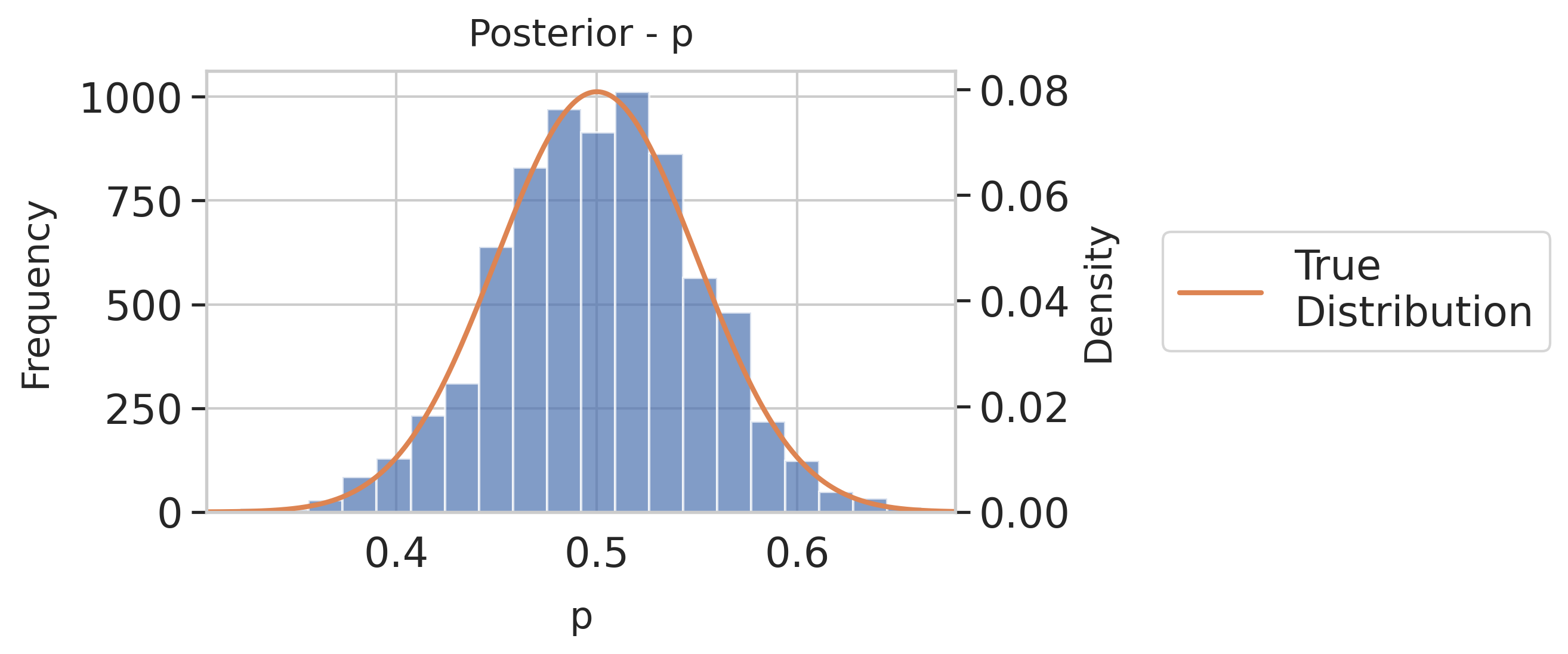
(a) Posterior distribution

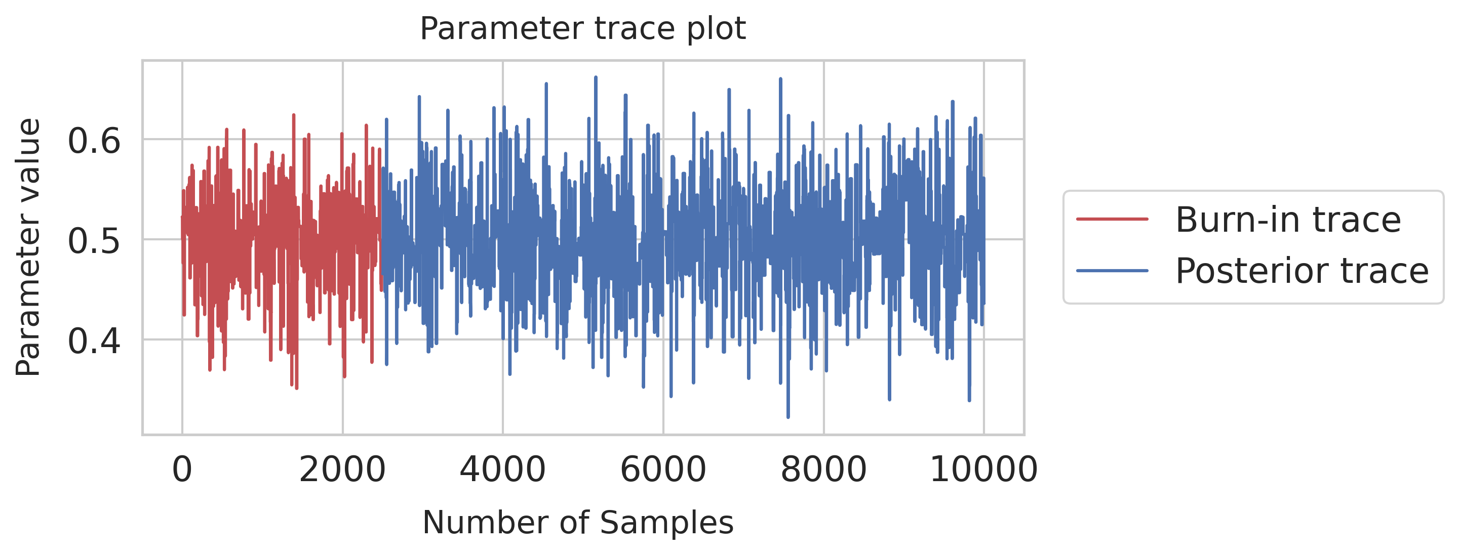
(b) Trace plot

Figure 6: Posterior and trace plot for the basic MCMC sampler example.

4 Bayesian linear models via MCMC

We give details of implementing Bayesian logistic regression that uses Metropolis-Hastings MCMC with random-walk proposal distribution.

We wish to model a univariate timeseries consisting of observed data points with inputs $X=(\mathbf{x}_{1},\ldots,\mathbf{x}_{S})^{\prime}$. We assume that the relationship between inputs and outputs is a signal plus noise model where the signal depends upon a set of parameters $\theta$, denoted by $f(\mathbf{x},\theta)$. We assume the noise to be Gaussian with a mean of zero and a variance of $\tau^{2}$, so that

$$y=f(\mathbf{x},\theta)+e\qquad e\sim\mathcal{N}(0,\tau^{2})$$ (10)

or equivalently,

$$p(y|x,\theta,\tau^{2})\sim\mathcal{N}\left(f(\mathbf{x},\theta),\tau^{2}\right)$$ (11)

We have adopt above form to generalise to the neural network model later; hence, Equation 12 expresses the case of a linear model.

$$f(\mathbf{x},\theta)=\theta\mathbf{X}^{T}$$ (12)

In this linear regression problem, we then have the parameters $\theta$ (that represents all weights and biases) and $\tau$ (that represents a single noise parameter). We sample the parameters using MCMC to find their posterior distributions. Note that from an optimisation perspective, the case of sampling can be seen as a form of optimisation, eg. using gradient-based methods [100] for learning the parameters of linear models or neural networks, i.e similar to the case of training a perceptron model [101] in the machine learning and neural networks literature. The additional aspect of a MCMC sampler is their ability to sample a posterior probability distribution that represents the parameters of a model rather than a fixed point estimate given by optimisation methods.

4.1 Likelihood

As detailed above in Section 2.1, our Bayesian treatment of the problem of finding the posterior $p(\theta\mid y)$ requires the definition of both a likelihood $p(\theta\mid\mathbf{x})$ and prior distribution $p(\theta)$. We begin by defining the likelihood. The likelihood, i.e probability of the data given the model is given by the product of the likelihood for each of our data points ($S$ total) as shown in Equation 13.

$$p(y\mid x,\theta,\tau^{2})=\prod_{t=1}^{S}p(y_{t}\mid x_{t},\theta,\tau^{2})$$ (13)

We note that for MCMC implementation, we would be using log-likelihood (i.e taking the log of the likelihood function) to eliminate numerical instabilities which can occur since we multiple probabilities together which grows with the size of the data. It is also more convenient to maximize the log of the likelihood function since the logarithm is monotonically increasing function of its argument, maximization of the log of a function is equivalent to maximization of the function itself. In order to transform a likelihood function into a log-likelihood, we will use the log product rule as given below.

$$log_{b}(x\times y)=log_{b}(x)+log_{b}(y)$$ (14)

The log-likelihood simplifies the subsequent mathematical analysis and also helps avoid numerical instabilities due to the product of a large number of small probabilities. In the log-likelihood, Equation 13 is much simplified by computing the sum of the log probabilities as given in Equation 15.

$$\ln p(y\mid x,\theta,\tau^{2})=\sum_{t=1}^{S}\ln p(y_{t}\mid x_{t},\theta,\tau^{2})$$ (15)

In order to construct the likelihood function, we use our definition of the probability for each data point given the model as shown in Equation 11, and the form of the Gaussian distribution as defined in Equation 3. We use a set of weights and biases as the model parameters $\boldsymbol{\theta}$ in our model $f(x,\theta)$ for $S$ training data instances and variance $\tau^{2}$. Our assumption of normally distributed errors leads to a likelihood given in Equation 16.

$$p(y\mid x,\theta,\tau^{2})=\frac{1}{(2\pi\tau^{2})^{S/2}}\times\exp\left(-\frac{1}{2\tau^{2}}\sum_{t=1}^{S}\left(y_{t}-f(x_{t},\theta)\right)^{2}\right)$$ (16)

4.2 Prior

We note that a linear model transforms into a Bayesian linear model with the use of a prior distribution, and a likelihood function to sample the posterior distribution via MCMC. In Section 3.2, we discussed the need to define a prior distribution for our model parameters $\theta$ and $\tau$. In the case where the prior distribution comes from the same probability distribution family as the posterior distribution, the prior and posterior are then called conjugate distributions [102, 103]. The prior is called a conjugate prior for the likelihood function of the Bayesian model.

To implement conjugate priors in our linear model, we will assume a multivariate Gaussian prior for $theta$ (Equation 17) and an inverse Gamma distribution (IG) for $\tau^{2}$ (Equation 18) . We use an IG prior distribution since we require positive real numbers to represent $\tau^{2}$. We use the multivariate Gaussian distribution to represent the parameters such as weights and bias of the linear models. These parameters feature negative and positive real number values and we are involving a model with more than one parameter, hence the multivariate Gaussian distribution is most appropriate for the prior.

$$\theta\sim\mathcal{N}(0,\sigma^{2})$$ (17)

$$\tau^{2}\sim IG(\nu_{1},\nu_{2})$$ (18)

In this example, we choose parameter values of $\sigma=5$, $\nu_{1}=0$, and $\nu_{2}=0$ to define the prior distributions. These values are based on expert opinion who consider trained models.

First, lets revisit multivariate normal distribution from Equation 4, used here to define the prior distribution for our weights and biases. Suppose that our $\mathbf{x}$ is our set of $M$ weights and biases, $(\theta_{1},\ldots,\theta_{M})$. Suppose our $\mathbf{\mu}$ is a vector of zeros (as defined above), then we get:

$$f(\theta_{1},\ldots,\theta_{M})=\frac{1}{\sqrt{(2\pi)^{M}|\boldsymbol{\Sigma}|}}\exp\left(-\frac{1}{2}({\boldsymbol{\theta}})^{\mathrm{T}}{\boldsymbol{\Sigma}}^{-1}({\boldsymbol{\theta}})\right)$$ (19)

The covariance matrix $\mathbf{\Sigma}$ in this case is just a diagonal matrix with all values equal to $\sigma^{2}$ (scalar), ${\mathbf{\Sigma}}^{-1}$ will become $I/\sigma^{2}$ where $I$ is an identity matrix (diagonal elements which are all ones). Hence, the numerator in above equation

$$({\boldsymbol{\theta}})^{\mathrm{T}}{\boldsymbol{\Sigma}}^{-1}({\boldsymbol{\theta}})$$ (20)

becomes

$$\frac{({\boldsymbol{\theta}})^{\mathrm{T}}{\mathbf{I}}({\boldsymbol{\theta}})}{\sigma^{2}}$$ (21)

We note that multiplying identity matrix with any other matrix is the matrix itself, hence finally we get ${\mathbf{\theta}}^{2}$ in numerator. We can now move to the IG distribution used to define the prior for our model variance ($\tau^{2}$).

$$f(\tau^{2})=\frac{\nu_{1}^{\nu_{2}}}{\Gamma(\nu_{1})}\left(\frac{1}{\tau^{2}}\right)^{\nu_{1}+1}\exp\left(\frac{-\nu_{2}}{\tau^{2}}\right)$$ (22)

We note that $\nu_{1}^{\nu_{2}}/\Gamma(\nu_{1})$ is a constant which can be dropped considering proportionality.

Equation 23 takes into account the product of all our MCMC parameters to define the overall prior.

$$p(\boldsymbol{\theta})\propto\frac{1}{(2\pi\sigma^{2})^{M/2}}\times\exp\Bigg{\{}-\frac{1}{2\sigma^{2}}\bigg{(}\sum_{i=1}^{M}\theta^{2}\bigg{)}\Bigg{\}}\times\tau^{-2(1+\nu_{1})}\exp\left(\frac{-\nu_{2}}{\tau^{2}}\right)$$ (23)

4.3 Python Implementation

The following code presented in Listing LABEL:lst:linar-reg-model implements a model in the form outlined above. First, we will define our simple linear model as in Equation 12.

⬇

1class LinearModel:

2 ’’’

3 Simple linear model with a single output (y) given the covariates x_1...x_M of the form:

4 y = w_1 * x_1 + ... + w_M * x_M + b

5 where M = number of features, w are the weights, and b is the bias.

6 ’’’

7 # Initialise values of model parameters

8 def __init__(self):

9 self.w = None

10 self.b = None

11

12 # Function to take in data and parameter sample and return the prediction

13 def evaluate_proposal(self, data, theta):

14 ’’’

15 Encode the proposed parameters and then use the model to predict

16 Input:

17 data: (N x M) array of data

18 theta: (M + 1) vector of parameters. The last element of theta consitutes the bias term (giving M + 1 elements)

19 ’’’

20 self.encode(theta) # method to encode w and b

21 prediction = self.predict(data) # predict and return

22 return prediction

23

24 # Linear model prediction

25 def predict(self, x_in):

26 y_out = x_in.dot(self.w) + self.b

27 return y_out

28

29 # Helper function to split the parameter vector into w and band store in the model

30 def encode(self, theta):

31 self.w = theta[0:-1]

32 self.b = theta[-1]

Listing 5: Python implementation of a simple linear regression model

Now that we have a class for our model, we should next define the functions that will allow us to carry out MCMC sampling over our model parameters. First we will need to define our likelihood function (Equation 16) which, when taking the log becomes:

$$logp(y\mid x,\theta,\tau^{2})=-log((2\pi\tau^{2})^{S/2})-\frac{1}{2\tau^{2}}\sum_{t=1}^{S}\left(y_{t}-f(x_{t},\theta)\right)^{2}$$ (24)

and prior likelihood (Equation 23), again taking the log giving:

$$logp(\boldsymbol{\theta})\propto\frac{1}{(2\pi\sigma^{2})^{M/2}}\times\exp\Bigg{\{}-\frac{1}{2\sigma^{2}}\bigg{(}\sum_{i=1}^{M}\theta^{2}\bigg{)}\Bigg{\}}\times\tau^{-2(1+\nu_{1})}\exp\left(\frac{-\nu_{2}}{\tau^{2}}\right)$$ (25)

⬇

1# Define the likelihood function

2def likelihood_function(self, theta, tausq):

3 ’’’

4 Calculate the likelihood of the data given the parameters

5 Input:

6 theta: (M + 1) vector of parameters. The last element of theta consitutes the bias term (giving M + 1 elements)

7 tausq: variance of the error term

8 Output:

9 log_likelihood: log likelihood of the data given the parameters

10 model_prediction: prediction of the model given the parameters

11 accuracy: accuracy (RMSE) of the model given the parameters

12 ’’’

13 # first make a prediction with parameters theta

14 model_prediction = self.model.evaluate_proposal(self.x_data, theta)

15 accuracy = self.rmse(model_prediction, self.y_data) #RMSE error metric

16 # now calculate the log likelihood

17 log_likelihood = np.sum(-0.5 * np.log(2 * np.pi * tausq) - 0.5 * np.square(self.y_data - model_prediction) / tausq)

18 return [log_likelihood, model_prediction, accuracy]

19

20# Define the prior

21def prior_likelihood(self, sigma_squared, nu_1, nu_2, theta, tausq):

22 ’’’

23 Calculate the prior likelihood of the parameters

24 Input:

25 sigma_squared: variance of normal prior for theta

26 nu_1: parameter nu_1 of the inverse gamma prior for tau^2

27 nu_2: parameter nu_2 of the inverse gamma prior for tau^2

28 theta: (M + 1) vector of parameters. The last element of theta consitutes the bias term (giving M + 1 elements)

29 tausq: variance of the error term

30 Output:

31 log_prior: log prior likelihood

32 ’’’

33 n_params = self.theta_size # number of parameters in model

34 part1 = -1 * (n_params / 2) * np.log(sigma_squared)

35 part2 = 1 / (2 * sigma_squared) * (sum(np.square(theta)))

36 log_prior = part1 - part2 - (1 + nu_1) * np.log(tausq) - (nu_2 / tausq)

37 return log_prior

Listing 6: Python implementation of likelihood and prior functions for linear regression model to be incorporated into the MCMC sampling class

Before running MCMC, we need to set up the sampler. First we generate an initial sample for our parameters, and initialise arrays to capture the samples that form the posterior distribution, the accuracy, and the model predictions. Then we proceed with sampling as per the MCMC sampling algorithm detailed in Algorithm 1. This algorithm uses a Gaussian random walk for the parameter proposals ($\theta_{p}$ and $\tau^{2}_{p}$), perturbing the previous proposed value with Gaussian noise as shown in Equations 26 and 27, respectively.

$$\theta_{p}\sim\theta_{p-1}+\mathcal{N}(0,\sigma_{\theta})$$ (26)

$$\tau^{2}_{p}\sim\tau^{2}_{p-1}+\mathcal{N}(0,\sigma_{\tau^{2}})$$ (27)

We then accept/reject the proposed value according to the Metropolis-Hastings acceptance ratio. Note that the log-likelihood is used and hence the ratio of previous and current likelihood will need to consider log laws (rules), i.e we note the log product rule in Equation 28 and the quotient rule in Equation 29.

$$log_{b}(x\times y)=log_{b}(x)+log_{b}(y)$$ (28)

$$log_{b}(x/y)=log_{b}(x)-log_{b}(y)$$ (29)

⬇

1# MCMC sampler

2def sampler(self):

3 ’’’

4 Run the sampler for a defined linear model

5 ’’’

6 ## Define empty arrays to store the sampled posterior values

7 # posterior of all weights and bias over all samples

8 pos_theta = np.ones((self.n_samples, self.theta_size))

9 # posterior defining the variance of the noise in predictions

10 pos_tau = np.ones((self.n_samples, 1))

11

12 # record output f(x) over all samples

13 pred_y = np.ones((self.n_samples, self.x_data.shape[0]))

14 # record the RMSE of each sample

15 rmse_data = np.zeros(self.n_samples)

16

17 ## Initialisation

18 # initialise theta - the model parameters

19 theta = np.random.randn(self.theta_size)

20 # make initial prediction

21 pred_y[0,] = self.model.evaluate_proposal(self.x_data, theta)

22

23 # initialise eta - we sample eta as a gaussian random walk in the log space of tau^2

24 eta = np.log(np.var(pred_y[0,] - self.y_data))

25 tausq_proposal = np.exp(eta)

26

27 # calculate the prior likelihood

28 prior_likelihood = self.prior_likelihood(self.sigma_squared, self.nu_1, self.nu_2, theta, tausq_proposal)

29 # calculate the likelihood considering observations

30 [likelihood, pred_y[0,], _, rmse_data[0]] = self.likelihood_function(theta, tausq_proposal)

31

32 n_accept = 0

33 ## Run the MCMC sample for n_samples

34 for ii in np.arange(1,self.n_samples):

35 # Sample new values for theta and tau using a Gaussian random walk

36 theta_proposal = theta + np.random.normal(0, self.step_theta, self.theta_size)

37 eta_proposal = eta + np.random.normal(0, self.step_eta, 1) # sample tau^2 in log space

38 tausq_proposal = np.exp(eta_proposal)

39

40 # calculate the prior likelihood

41 prior_proposal = self.prior_likelihood(

42 self.sigma_squared, self.nu_1, self.nu_2, theta_proposal, tausq_proposal

43 )

44 # calculate the likelihood considering observations

45 [likelihood_proposal, pred_y[ii,], _, rmse_data[ii]] = self.likelihood_function(

46 theta_proposal, tausq_proposal

47 )

48

49 # Noting that likelihood_function and prior_likelihood return log likelihoods,

50 # we can use log laws to calculate the acceptance probability

51 diff_likelihood = likelihood_proposal - likelihood

52 diff_priorlikelihood = prior_proposal - prior_likelihood

53

54 mh_prob = min(1, np.exp(diff_likelihood + diff_priorlikelihood))

55

56 # sample to accept or reject the proposal according to the acceptance probability

57 u = np.random.uniform(0, 1)

58 if u < mh_prob:

59 # accept and update the values

60 n_accept += 1

61 likelihood = likelihood_proposal

62 prior_likelihood = prior_proposal

63 theta = theta_proposal

64 eta = eta_proposal

65 # store to make up the posterior

66 pos_theta[ii,] = theta_proposal

67 pos_tau[ii,] = tausq_proposal

68 else:

69 # reject move and store the old values

70 pos_theta[ii,] = pos_theta[ii-1,]

71 pos_tau[ii,] = pos_tau[ii-1,]

72

73 # calculate the acceptance rate as a check

74 accept_rate = (n_accept / self.n_samples) * 100

75 print(’{:.3f}% were accepted’.format(accept_rate))

76

77 # store the posterior (samples after burn in) in a pandas dataframe and return

78 self.pos_theta = pos_theta[self.n_burnin:, ]

79 self.pos_tau = pos_tau[self.n_burnin:, ]

80 self.rmse_data = rmse_data[self.n_burnin:]

81

82 # split theta into w and b

83 results_dict = {’w{}’.format(_): self.pos_theta[:, _].squeeze() for _ in range(self.theta_size-1)}

84 results_dict[’b’] = self.pos_theta[:, -1].squeeze()

85 results_dict[’tau’] = self.pos_tau.squeeze()

86 results_dict[’rmse’] = self.rmse_data.squeeze()

87

88 results_df = pd.DataFrame.from_dict(

89 results_dict

90 )

91 return results_df

Listing 7: Python implementation of an MCMC sampler for the linear model

Now that we have the sampler, we can create an MCMC class that brings together the model, data, hyperparameters and sampling algorithm.

⬇

1class MCMC:

2 def __init__(self, n_samples, n_burnin, x_data, y_data):

3 self.n_samples = n_samples # number of MCMC samples

4 self.n_burnin = n_burnin # number of burn-in samples

5 self.x_data = x_data # (N x M)

6 self.y_data = y_data # (N x 1)

7 self.theta_size = x_data.shape[1] + 1 # weights for each feature and a bias term (M+1)

8

9 # MCMC parameters - defines the variance term in our Gaussian random walk

10 self.step_theta = 0.02;

11 self.step_eta = 0.01; # note eta is used as tau in the sampler to consider log scale.

12

13 # model hyperparameters

14 # considered by looking at distribution of similar trained models - i.e distribution of weights and bias

15 self.sigma_squared = 5

16 self.nu_1 = 0

17 self.nu_2 = 0

18

19 # initisalise the linear model class

20 self.model = LinearModel()

21

22 # store output

23 self.pos_theta = None

24 self.pos_tau = None

25 self.rmse_data = None

26

27 # functions defined above - this is poor practice, but done for readability

28 # and clarity

29 self.likelihood_function = MethodType(likelihood_function, self)

30 self.prior_likelihood = MethodType(prior_likelihood, self)

31 self.sampler = MethodType(sampler, self)

32

33 def model_draws(self, num_samples = 10):

34 ’’’

35 Simulate new model predictions (mu) under the assumption that our posteriors are

36 Gaussian.

37 ’’’

38 # num_samples x num_data_points

39 pred_y = np.zeros((num_samples,self.x_data.shape[0]))

40 sim_y = np.zeros((num_samples,self.x_data.shape[0]))

41

42 for ii in range(num_samples):

43 theta_drawn = np.random.normal(self.pos_theta.mean(axis=0), self.pos_theta.std(axis=0), self.theta_size)

44 tausq_drawn = np.random.normal(self.pos_tau.mean(), self.pos_tau.std())

45

46 [_, pred_y[ii,:], sim_y[ii,:],_] = self.likelihood_function(

47 theta_drawn, tausq_drawn

48 )

49 return pred_y, sim_y

50

51 # Additional error metric

52 def rmse(self, predictions, targets):

53 return np.sqrt(((predictions - targets) ** 2).mean())

Listing 8: Python implementation of an MCMC class for fitting a linear regression model

We can then run the MCMC sampler.

⬇

1## MCMC Settings and Setup

2n_samples = 20000 # number of samples to draw from the posterior

3burn_in = int(n_samples* 0.25) # number of samples to discard before recording draws from the posterior

4

5# Generate toy data

6n_data = 100

7n_features = 1

8x_data = np.repeat(np.expand_dims(np.linspace(0, 1, n_data),axis=-1),n_features,axis=1)

9y_data = 3 * x_data[:,0] + 4 + np.random.randn(n_data) * 0.5

10

11# Initialise the MCMC class

12mcmc = MCMC(n_samples, burn_in, x_data, y_data)

13# Run the sampler

14results = mcmc.sampler()

15# Draw sample models from the posterior

16pred_y, sim_y = mcmc.model_draws(num_samples=100)

Listing 9: Code to call the MCMC sampling class and fit a model to some toy data

After the code runs, we can see the predictions of the trained Bayesian linear model and simulated values (model fit with added variance according to $\tau^{2}$), such as below in Figure 7.

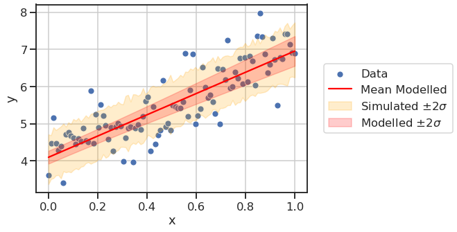
Figure 7: Bayesian linear regression model fitting a toy dataset.

5 Bayesian neural networks via MCMC

5.1 Neural networks

We utilise a simple neural network, also known as a multilayer perceptron to demonstrate the process of training a Bayesian neural network via MCMC. A neural network model $f(x)$ is made up of a series of lower level computations which can be used to transform inputs to their corresponding outputs $\{\bf\bar{x}_{t},\bf{y}_{t}\}$. Neural networks are structured as layers of neurons whose value is determined based on a linear combination of inputs from the previous layer, with an activation function used to introduce nonlinearity. In this case, we consider a neural network with one hidden layer and one output, as shown in Figure 8.

As an example, we can calculate the output value of the jth neuron in the first hidden layer of a network ($h,j$) using a weighted combination of the $m$ inputs ($\bar{x}_{t}$) as shown in Equation 30.

$$g\bigg{(}\delta_{h,j}+\sum_{i=1}^{m}w_{i,j}\bar{x}_{t,i}\bigg{)}$$ (30)

where, the bias ($\delta_{h,j}$) and weights ($w_{i}$ for each of the $m$ inputs) are parameters to be estimated (trained), and $g(.)$ is the activation function that can be used to perform a nonlinear transformation. In our case, the function $g(.)$ is the sigmoid activation function, used for the hidden and output layers of the neural network model with a single hidden layer as shown in Figure 8.

We train the model to approximate the function $f$ such that $f(\bf\bar{x}_{t})=\bf{y}_{t}$ for all pairs. We extend our previous calculation a single neuron in the hidden layer to calculate the output $f(\bf\bar{x}_{t})$ as shown in Equation 31.

$$f({\bf\bar{x}}_{t})=g\bigg{(}\delta_{o}+\sum_{j=1}^{H}v_{h}\times g\bigg{(}\delta_{h}+\sum_{i=1}^{m}w_{i,j}\bar{x}_{t,i}\bigg{)}\bigg{)},$$ (31)

where $H$ is the number of neurons in the hidden layer, $\delta_{o}$ is the bias for the output, and $v_{h}$ are the weights from the hidden layer to the output neuron. The complete set of parameters for the neural network model, shown in Figure 8, is made up of $\theta=(\mathbf{\tilde{w}},\mathbf{\tilde{v}},{\boldsymbol{\delta}})$, where ${\boldsymbol{\delta}}=({\boldsymbol{\delta}_{o}},{\boldsymbol{\delta}_{h}})$. $\mathbf{\tilde{w}}$ are the weights transforming the input to hidden layer. $\mathbf{\tilde{v}}$ are the weights transforming the hidden to output layer. ${\boldsymbol{\delta}_{h}}$ is the bias for the hidden layer, and ${\boldsymbol{\delta}_{o}}$ is the bias for the output layer.

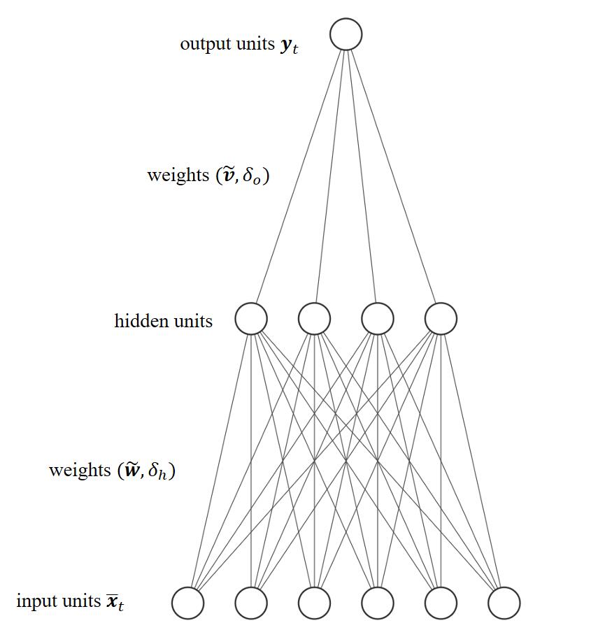
Figure 8: Simple neural network with a single hidden layer. The information is passed and processed from the input to hidden and then finally to the output layer as shown.

5.2 Bayesian neural networks

A Bayesian neural network is a probabilistic implementation of a standard neural network with the key difference being that the weights and biases are represented via the posterior probability distributions rather than single point values as shown in Figure 9. Similar to canonical neural networks [104], Bayesian neural networks also have universal continuous function approximation capabilities. However, the posterior distribution of the network parameters allows uncertainty quantification on the predictions.

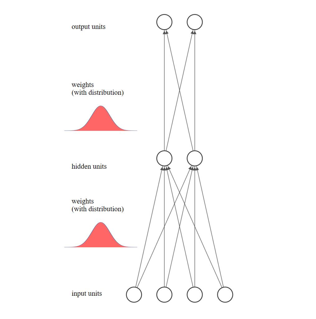
(a) Bayesian neural network

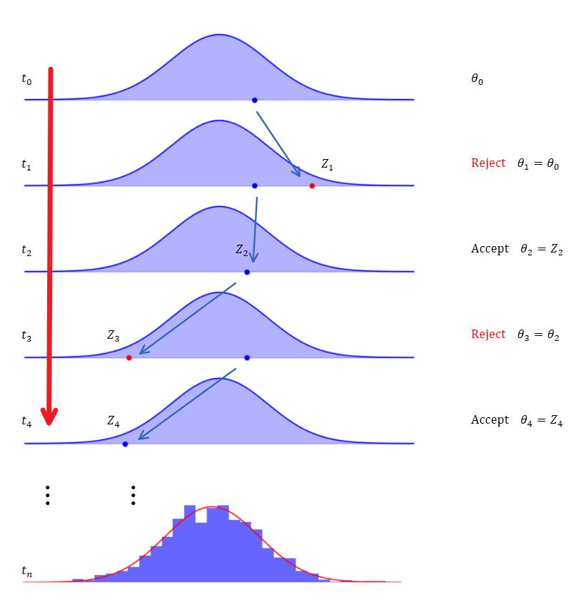
(b) MCMC sampling

Figure 9: Bayesian neural network and MCMC sampling. Adapted from [105].

The task for MCMC sampling is to learn (sample) the posterior distributions representing the weights and biases of the neural network that best fit the data. As in the previous examples, we begin inference with prior distributions over the weights and biases of the network and use a sampling scheme to find the posterior distributions given training data. Since non-linear activation functions exist in the network, the conjugacy of prior and posterior is lost, and therefore we must employ an MCMC sampling scheme and make assumptions about the distribution of errors.

We specify the model similar to the Bayesian linear regression, assuming a Gaussian error as given in Equation 32.

$$y=f(\mathbf{x},\theta)+e\qquad e\sim\mathcal{N}(0,\tau^{2})$$ (32)

This leads to the same likelihood function as presented in logarithmic form in Equation 24. As in Section 4.2, we adopt Gaussian priors for all parameters of the model ($\theta$), with zero mean and a user-defined variance ($\sigma^{2}$), and an IG distribution for the variance of the error model ($\tau^{2}$), with parameters $\nu_{1}$ and $\nu_{2}$. The likelihood function and prior likelihood function, therefore remain unchanged from their definition in Listing 6.

5.3 Training neural networks via backpropagation

We note that typically random-walk proposal distributions are used for small scale-models; however, neural network models features a large number of parameters. The choice of a proposal distribution is essential for models with large number of parameters. To better guide the sampling, we can incorporate gradients to our proposals and we will start by examining how gradients are incorporated in non-probabilistic deep learning problems.

Gradient based methods are widely used in deep learning alongside backpropagation to train models with various neural network architectures [106]. Stochastic gradient descent (SGD) involves stepping through the parameter space iteratively, guided by gradients, to optimize a differentiable objective function. The method has prominently featured in the training of various neural networks architectures including deep learning models. SGD is combined with backpropagation when training neural networks [107, 108, 109]. Backpropagation involves a forward pass which propagates information forward to get prediction (decision) at the output layer and a backward pass to compute the local gradients for each of the parameters. These gradients are then used to inform the update of the model parameters in an interative process, where the weights and biases are updated at each step. Training neural networks also can be considered as solving a non-convex optimization problem $\arg\!\min{L(\theta)}$; where, $\theta\in R^{n}$ is the set of parameters and $L$ is the loss function. The parameter (weight) update for an iteration (epoch) of SGD is shown in Equation 33.

$$\theta_{k}=\theta_{k-1}-a_{k-1}\nabla L(\theta_{k-1})$$ (33)

where, $\theta_{k}$ denotes the $k^{th}$ iteration, $a_{k}$ is the learning rate, and $\nabla L(\theta_{k})$ denotes the gradient.

We note that the learning rate is user defined hyperparameter which depends on the problem and data at hand. It is typically determined through tuning using cross-validation or trial and error. A number of extensions of the backgropagation algorithm employing SGD have been proposed to address limitations. These include use of weight decay regularization during training to improve generalisation ability [110], a momentum mechanism for faster training [111, 112], adaptive learning rate [112], and second order gradient methods [113] which, although efficient, have problems in scaling up computationally with larger models. In the last decade, with the deep learning revolution, further attempts have been made to ensure that enhanced backpropagation algorithms, not only improve training accuracy, but can also scale well computationally for large deep learning models. Hence, the development of methods such as the adaptive gradient algorithm (AdaGrad) [114], ada-delta [115], and Adam (adaptive moment estimation) [116]. These advanced algorithms are generally based on the idea of adapting the learning rate automatically during the training, taking into account the recent history of the optimisation process.

5.3.1 Langevin gradient-based proposal distribution

We mentioned earlier that random-walk proposal distributions are suited for small scale models and better proposal distributions would be required for neural network models. Although simple neural networks have much lower number of parameters, when compared to deep learning models, training simple neural networks with MCMC sampling is a challenge with random-walk proposal distribution. We need to utilise the properties of backpropagation algorithm and the mechanism of weight update using gradients. Hence, we utilise stochastic gradient Langevin dynamics [58] for the proposal distribution which features the addition of noise to the stochastic gradients. The method has shown to be effective for linear models [58] which motivated its use in Bayesian neural networks. In our previous work, Langevin-gradient MCMC has been very promising for simple and deep neural networks [59, 66, 65]. Hence, we draw the proposed values for the parameters ($\boldsymbol{\theta}^{p}$) according to a one-step (epoch) gradient as shown in Equation 34.

$$\boldsymbol{\theta}^{p}\sim\mathcal{N}(\bar{\boldsymbol{\theta}}^{[s]},\Sigma_{\theta})$$ (34)

A Gaussian distribution with a standard deviation of $\Sigma_{\theta}$, and mean ($\bar{\boldsymbol{\theta}}^{[s]}$) calculated using a gradient based update (Equation 35 of the parameter values from the previous step (${\boldsymbol{\theta}}^{[s]}$).

$$\bar{\boldsymbol{\theta}}^{[s]}=\boldsymbol{\theta}^{[s]}+r\times\nabla E(\boldsymbol{\theta^{[s]}})$$ (35)

with learning rate $r$ (a user-defined hyperparameter) and gradient update ($\nabla E(\boldsymbol{\theta}^{[s]})$) according to the model residuals.

$$E(\boldsymbol{\theta}^{[s]})=\sum_{t\in{\mathcal{T}}}(y_{t}-F({\bf x}_{i},\boldsymbol{\theta^{[s]}}))^{2}$$ (36)

$$\nabla E(\boldsymbol{\theta}^{[s]})=\left(\frac{\partial{E}}{\partial{\theta_{1}}},\ldots,\frac{\partial{E}}{\partial{\theta_{L}}}\right).$$

Hence, the Langevin gradient-based proposal consists of 2 parts:

1. Gradient descent-based weight update

2. Addition of Gaussian noise from $\mathcal{N}(0,\Sigma_{\theta})$

We need to ensure that the detailed balance is maintained since the Langevin-gradient proposals are not symmetric. We note that MCMC implementation with relaxed detailed balance condition for some applications also exist [117]. Therefore, a combined update is used as a proposal in a Metropolis-Hastings step, which accepts the proposal $\boldsymbol{\theta}^{p}$ for a position $s$ with the probability $\alpha$ as shown in Equation 37.

$$\alpha=\min\left\{1,\frac{p(\boldsymbol{\theta}^{p}|\mathbf{y})q(\boldsymbol{\theta}^{[s]}|\boldsymbol{\theta}^{p})}{p(\boldsymbol{\theta}^{[s]}|\mathbf{y})q(\boldsymbol{\theta}^{p}|\boldsymbol{\theta}^{[s]})}\right\}$$ (37)

where, $p(\boldsymbol{\theta}^{p}|\mathbf{y})$ and $p(\boldsymbol{\theta}^{[s]}|\mathbf{y})$ can be computed using the likelihood from Equation (16), and priors given by Equation (23). The ratio of the proposed and the current $q(\boldsymbol{\theta}^{p}|\boldsymbol{\theta}^{[s]})$, is given by Equation 38 which is based on a one-step (epoch) gradient $\nabla E_{\bf y}[\boldsymbol{\theta}^{[s]}$ with user-defined learning rate $r$ given in Equation 39.

$$q(\boldsymbol{\theta}^{[s]}|\boldsymbol{\theta}^{p})\sim N(\bar{\boldsymbol{\theta}}^{[s]},\Sigma_{\boldsymbol{\theta}})$$ (38)

$$\bar{\boldsymbol{\theta}}^{[s]}=\boldsymbol{\theta}^{[s]}+r\times\nabla E_{\bf y}[\boldsymbol{\theta}^{[s]}]$$ (39)

Thus, this ensures that the detailed balance condition holds and the sequence ${\boldsymbol{\theta}}^{[s]}$ converges to draws from the posterior $p(\boldsymbol{\theta}|\bf y)$. Since our implementation is in the log-scale, the log posterior is given by 40.

$$\log\left(p(\boldsymbol{\theta}|{\bf y})\right)=\log\left(p(\boldsymbol{\theta})\right)+\log\left(p({\bf y}|\boldsymbol{\theta})\right)+log(q(\boldsymbol{\theta}|\boldsymbol{\theta^{*}}))$$ (40)

Algorithm 2 gives a full description of the Langevin-gradient MCMC sampling scheme, bringing together all the steps outlined above. User defined parameters are present for the maximum number of samples ($S_{max}$), rate of Langevin-gradient proposals ($L_{prob}$) compared to simple random walk proposals, and learning rate $r$ for Langevin-gradient proposals. We note that in a standard Langevin MCMC approach, the rate of it being used ($L_{prob}$) is 1 and Gaussian noise is already part of Langevin gradients. However, in our implementation, we use a combination of random-walk proposal distribution with Langevin gradients, as this seem to be computationally more efficient than Langevin gradients alone which consume extra computational time when computing gradients, especially in larger models.

We begin by drawing initial values for the $\theta$ from the prior distribution given in Equation (23) (Stage 1.1). A new proposal is drawn for $\theta^{p}$ (which incorporates the model weights and biases and $\tau^{2}$ from either a Langevin-gradient or random-walk proposal distribution (Stage 1.2). The proposal is evaluated using the Bayesian neural network (BNN) model with the likelihood function in Equation 16 (Stage 1.4). We also evaluate the likelihood for the prior given in Equation (23) (Stage 1.3). Using these likelihoods, we can check if the proposal should be accepted using Metropolis-Hastings condition (Stage 1.5 and 1.6). If accepted, the proposal becomes part of the chain, else we retain previous the last accepted state of the chain. We repeat the procedure until the maximum samples are reached ($S_{max}$). Finally, we execute post-sampling stage where we obtain the posterior distribution by concatenating the history of the samples in the chain.

Data: Dataset

Result: Posterior distribution of model parameters (weights and biases)

- Stage 1.0: Metropolis Transition

- 1.1 Draw initial values $\theta_{0}$ from the prior

for each $s$ until $S_{max}$ do

      

      1.2 Draw $\kappa$ from a Uniform-distribution [0,1]

       if $\kappa\leq L_{prob}$ then

             Use Langevin-gradient proposal distribution: $\boldsymbol{\theta}^{p}\sim\mathcal{N}(\bar{\boldsymbol{\theta}}^{[s]},\Sigma_{\theta})$

       end if

      else

             Use random-walk proposal distribution: $\boldsymbol{\theta}^{p}\sim\mathcal{N}(\boldsymbol{\theta}^{[s]},\Sigma_{\theta})$

       end if

      1.3 Evaluate prior given in Equation 23

       1.4 Evaluate log-likelihood given in Equation 16

       1.5 Compute the posterior probability for Metropolis-Hastings condition - Equation 40

       1.6 Draw $u$ from a Uniform-distribution [0,1]

       if $\log(u)\leq log(p({\bf y}|\boldsymbol{\theta}))$ then

             Accept replica state: $\theta^{[s+1]}\leftarrow\theta^{p}$

       end if

      else

             Reject and retain previous state: $\theta^{[s+1]}\leftarrow\theta^{[s]}$

       end if

      

end for

Algorithm 2 Bayesian neural network framework using Langevin-based MCMC sampling.

5.4 Python Implementation

We first define and implement the simple neural network module (class), and implement methods (functions) for the forward and backward pass to calculate the output of the network given a set of inputs. We need to compute the gradients, and update the model parameters given a model prediction and observations, respectively. Listings 10, 11 and 12 present an implementation of the Bayesian Neural Network and associated Langevin-gradient MCMC sampling scheme.

⬇

1# NN prediction

2def forward_pass(self, X):

3 ’’’

4 Take an input X and return the output of the network

5 Input:

6 - X: (N x num_features) array of input data

7 Output:

8 - self.l2_output: (N) array of output data f(x) which can be

9 compared to observations (Y)

10 ’’’

11 # Hidden layer

12 l1_z = np.dot(X, self.l1_weights) + self.l1_biases

13 self.l1_output = self.sigmoid(l1_z) # activation function g(.)

14 # Output layer

15 l2_z = np.dot(self.l1_output, self.l2_weights) + self.l2_biases

16 self.l2_output = self.sigmoid(l2_z)

17 return self.l2_output

18

19def backward_pass(self, X, Y):

20 ’’’

21 Compute the gradients using a backward pass and undertake Langevin-gradient updating of parameters

22 Input:

23 - X: (N x num_features) array of input data

24 - Y: (N) array of target data

25 ’’’

26 # dE/dtheta

27 l2_delta = (Y - self.l2_output) * (self.l2_output * (1 - self.l2_output))

28 l2_weights_delta = np.outer(

29 self.l1_output,

30 l2_delta

31 )

32 # backprop of l2_delta and same as above

33 l1_delta = np.dot(l2_delta,self.l2_weights.T) * (self.l1_output * (1 - self.l1_output))

34 l1_weights_delta = np.outer(

35 X,

36 l1_delta

37 )

38

39 # update for output layer

40 self.l2_weights += self.lrate * l2_weights_delta

41 self.l2_biases += self.lrate * l2_delta

42 # update for hidden layer

43 self.l1_weights += self.lrate * l1_weights_delta

44 self.l1_biases += self.lrate * l1_delta

Listing 10: Python implementation of Neural Network forward and backward passes

Next, we implement the model for a single hidden layer neural network with multiple input neurons and a single output neuron (one step ahead prediction).

⬇

1class NeuralNetwork:

2 ’’’

3 Neural Network model with a single hidden layer and a single output (y)

4 ’’’

5 def __init__(self, layer_sizes,learning_rate=0.01):

6 ’’’

7 Initialize the model

8 Input:

9 - layer_sizes (input, hidden, output): array specifying the number of

10 nodes in each layer

11 - learning_rate: learning rate for the gradient update

12 ’’’

13 # Initial values of model parameters

14 self.input_num = layer_sizes[0]

15 self.hidden_num = layer_sizes[1]

16 self.output_num = layer_sizes[2]

17

18 # total number of parameters from weights and biases

19 self.n_params = (self.input_num * self.hidden_num) + (self.hidden_num * self.output_num) +\

20 self.hidden_num + self.output_num

21 # learning params

22 self.lrate = learning_rate

23

24 # Initialize network structure

25 self.initialise_network()

26

27 # functions defined above - this is poor practice, but done for readability

28 # and clarity

29 self.forward_pass = MethodType(forward_pass, self)

30 self.backward_pass = MethodType(backward_pass, self)

31

32 def initialise_network(self):

33 ’’’

34 Initialize network structure - weights and biases for the hidden layer

35 and output layer

36 ’’’

37 # hidden layer

38 self.l1_weights = np.random.normal(

39 loc=0, scale=1/np.sqrt(self.input_num),

40 size=(self.input_num, self.hidden_num))

41 self.l1_biases = np.random.normal(

42 loc=0, scale=1/np.sqrt(self.hidden_num),

43 size=(self.hidden_num,))

44 # placeholder for storing the hidden layer values

45 self.l1_output = np.zeros((1, self.hidden_num))

46

47 # output layer

48 self.l2_weights = np.random.normal(

49 loc=0, scale=1/np.sqrt(self.hidden_num),

50 size=(self.hidden_num, self.output_num))

51 self.l2_biases = np.random.normal(

52 loc=0, scale=1/np.sqrt(self.hidden_num),

53 size=(self.output_num,))

54 # placeholder for storing the model outputs

55 self.l2_output = np.zeros((1, self.output_num))

56

57 def evaluate_proposal(self, x_data, theta):

58 ’’’

59 A helper function to take the input data and proposed parameter sample

60 and return the prediction

61 Input:

62 data: (N x num_features) array of data

63 theta: (w,v,b_h,b_o) vector of parameters with weights and biases

64 ’’’

65 self.decode(theta) # method to decode w into W1, W2, B1, B2.

66 size = x_data.shape[0]

67

68 fx = np.zeros(size)

69

70 for i in range(0, size): # to see what fx is produced by your current weight update

71 fx[i] = self.forward_pass(x_data[i,])

72

73 return fx

74

75 def langevin_gradient(self, x_data, y_data, theta, depth):

76 ’’’

77 Compute the Langevin gradient based proposal distribution

78 Input:

79 - x_data: (N x num_features) array of input data

80 - y_data: (N) array of target data

81 - theta: (w,v,b_h,b_o) vector of proposed parameters.

82 - depth: SGD depth

83 Output:

84 - theta_updated: Updated parameter proposal

85

86 ’’’

87 self.decode(theta) # method to decode w into W1, W2, B1, B2.

88 size = x_data.shape[0]

89 # Update the parameters based on LG

90 for _ in range(0, depth):

91 for ii in range(0, size):

92 self.forward_pass(x_data[ii,])

93 self.backward_pass(x_data[ii,], y_data[ii])

94 theta_updated = self.encode()

95 return theta_updated

96

97 # Helper functions

98 def sigmoid(self, x):

99 ’’’

100 Implentation of the sigmoid function

101 ’’’

102 return 1 / (1 + np.exp(-x))

103

104 def encode(self):

105 ’’’

106 Encode the model parameters into a vector

107 Output:

108 - theta: vector of parameters.

109 ’’’

110 w1 = self.l1_weights.ravel()

111 w2 = self.l2_weights.ravel()

112 theta = np.concatenate([w1, w2, self.l1_biases, self.l2_biases])

113 return theta

114

115 def decode(self, theta):

116 ’’’

117 Decode the model parameters from a vector

118 Input:

119 - theta: vector of parameters.

120 ’’’

121 w_layer1size = self.input_num * self.hidden_num

122 w_layer2size = self.hidden_num * self.output_num

123

124 w_layer1 = theta[0:w_layer1size]

125 self.l1_weights = np.reshape(w_layer1, (self.input_num, self.hidden_num))

126

127 w_layer2 = theta[w_layer1size:w_layer1size + w_layer2size]

128 self.l2_weights = np.reshape(w_layer2, (self.hidden_num, self.output_num))

129 self.l1_biases = theta[w_layer1size + w_layer2size:w_layer1size + w_layer2size + self.hidden_num]

130 self.l2_biases = theta[w_layer1size + w_layer2size + self.hidden_num:w_layer1size + w_layer2size + self.hidden_num + self.output_num]

Listing 11: Python implementation of the Neural Network class

Finally, we implement an MCMC sampler following the Langevin-gradient MCMC sampling scheme. As discussed above, the prior and likelihood functions remain the same as in the linear regression model case, as presented in Listing 6.

⬇

1# MCMC sampler

2def sampler(self):

3 ’’’

4 Run the sampler for a defined Neural Network model

5 ’’’

6 # define empty arrays to store the sampled posterior values

7 # posterior of all weights and bias over all samples

8 pos_theta = np.ones((self.n_samples, self.theta_size))

9 # posterior defining the variance of the noise in predictions

10 pos_tau = np.ones((self.n_samples, 1))

11

12 # record output f(x) over all samples

13 pred_y = np.ones((self.n_samples, self.x_data.shape[0]))

14 # record simulated values f(x) + error over all samples

15 sim_y = np.ones((self.n_samples, self.x_data.shape[0]))

16 # record the RMSE of each sample

17 rmse_data = np.zeros(self.n_samples)

18

19 ## Initialisation

20 # initialise theta

21 theta = np.random.randn(self.theta_size)

22 # make initial prediction

23 pred_y[0,] = self.model.evaluate_proposal(self.x_data, theta)

24

25 # initialise eta

26 eta = np.log(np.var(pred_y[0,] - self.y_data))

27 tau_proposal = np.exp(eta)

28

29 # Hyperpriors - considered by looking at distribution of similar trained models - i.e distribution of weights and bias

30 sigma_squared = self.sigma_squared

31 nu_1 = self.nu_1

32 nu_2 = self.nu_2

33

34 # calculate the prior likelihood

35 prior_likelihood = self.prior_likelihood(sigma_squared, nu_1, nu_2, theta, tau_proposal)

36 # calculate the likelihood considering observations

37 [likelihood, pred_y[0,], sim_y[0,], rmse_data[0]] = self.likelihood_function(theta, tau_proposal)

38

39 n_accept = 0

40 n_langevin = 0

41 # Run the MCMC sample for n_samples

42 for ii in tqdm(np.arange(1,self.n_samples)):

43 # Sample new values for theta and tau

44 theta_proposal = theta + np.random.normal(0, self.step_theta, self.theta_size)

45

46 lx = np.random.uniform(0,1,1)

47 if (self.use_langevin_gradients is True) and (lx < self.l_prob):

48 theta_gd = self.model.langevin_gradient(self.x_data, self.y_data, theta.copy(), self.sgd_depth)

49 theta_proposal = np.random.normal(theta_gd, self.step_theta, self.theta_size)

50 theta_proposal_gd = self.model.langevin_gradient(self.x_data, self.y_data, theta_proposal.copy(), self.sgd_depth)

51

52 # for numerical reasons, we will provide a simplified implementation that simplifies

53 # the MVN of the proposal distribution

54 wc_delta = (theta - theta_proposal_gd)

55 wp_delta = (theta_proposal - theta_gd)

56

57 sigma_sq = self.step_theta

58

59 first = -0.5 * np.sum(wc_delta * wc_delta) / sigma_sq # this is wc_delta.T * wc_delta /sigma_sq

60 second = -0.5 * np.sum(wp_delta * wp_delta) / sigma_sq

61

62 diff_prop = first - second

63 n_langevin += 1

64 else:

65 diff_prop = 0

66 theta_proposal = np.random.normal(theta, self.step_theta, self.theta_size)

67

68 # eta proposal

69 eta_proposal = eta + np.random.normal(0, self.step_eta, 1)

70 tau_proposal = np.exp(eta_proposal)

71

72 # calculate the prior likelihood

73 prior_proposal = self.prior_likelihood(

74 sigma_squared, nu_1, nu_2, theta_proposal, tau_proposal

75 ) # takes care of the gradients

76 # calculate the likelihood considering observations

77 [likelihood_proposal, pred_y[ii,], sim_y[ii,], rmse_data[ii]] = self.likelihood_function(

78 theta_proposal, tau_proposal

79 )

80

81 # since we using log scale: based on https://www.rapidtables.com/math/algebra/Logarithm.html

82 diff_likelihood = likelihood_proposal - likelihood

83 diff_priorlikelihood = prior_proposal - prior_likelihood

84

85 mh_prob = min(1, np.exp(diff_likelihood + diff_priorlikelihood + diff_prop))

86

87 u = np.random.uniform(0, 1)

88

89 # Accept/reject

90 if u < mh_prob:

91 # Update position

92 n_accept += 1

93 # update

94 likelihood = likelihood_proposal

95 prior_likelihood = prior_proposal

96 theta = theta_proposal

97 eta = eta_proposal

98 # and store

99 pos_theta[ii,] = theta_proposal

100 pos_tau[ii,] = tau_proposal

101 else:

102 # store

103 pos_theta[ii,] = pos_theta[ii-1,]

104 pos_tau[ii,] = pos_tau[ii-1,]

105

106 # print the % of times the proposal was accepted

107 accept_ratio = (n_accept / self.n_samples) * 100

108 print(accept_ratio, ’% was accepted’)

109

110 # store the posterior of theta and tau, as well as the RMSE of these samples

111 self.pos_theta = pos_theta[self.n_burnin:, ]

112 self.pos_tau = pos_tau[self.n_burnin:, ]

113 self.rmse_data = rmse_data[self.n_burnin:]

114

115 # Create a pandas dataframe to store the posterior samples of theta and tau, the

116 # associated RMSE

117 results_dict = {’w{}’.format(_): self.pos_theta[:, _].squeeze() for _ in range(self.theta_size-2)}

118 results_dict[’b0’] = self.pos_theta[:, self.theta_size-2].squeeze()

119 results_dict[’b1’] = self.pos_theta[:, self.theta_size-1].squeeze()

120 results_dict[’tau’] = self.pos_tau.squeeze()

121 results_dict[’rmse’] = self.rmse_data.squeeze()

122

123 results_df = pd.DataFrame.from_dict(

124 results_dict

125 )

126 return results_df

Listing 12: Python implementation MCMC sampler - Langevin proposal distribution

5.5 Results

We use the Sunspot time series data and Abalone datasets for regression problems. The Abalone dataset provides the ring age for Abalone based on eight features that represent physical properties such as length, width, and weight and associated target feature, i.e., the ring age. Determining the age of Abalone is difficult as requires cutting the shell and counting the number of rings using a microscope. However, other physical measurements can be used to predict the age and a model can be developed to use the physical features to determine the ring age. Sunspots are regions of reduced surface temperature in the Sun’s photosphere caused by concentrations of magnetic field flux, and appear as spots darker than the surrounding areas. The Sunspot cycles are about every eleven years and over the solar cycle, the number of occurrence of Sunspot change more rapidly. Sunspot activities are monitored since they have an include on Earth’s climate and weather systems. We obtain the Abalone dataset from the University of California (UCI) Machine Learning Repository and keep a processed version of all the datasets in our repository. We also obtain datasets for classification problems from the same repository that features a number of datasets, but we only close Iris and Ionosphere classification data. The Iris classification dataset contains 4 features (sepal length, sepal width, petal length, petal with) of three types of Iris flower species, featuring 50 instances for each case. This dataset is one of the most prominent datasets used for machine learning. In the Ionosphere dataset, there are 34 continuous features and the target is either ”good” or ”bad”, a binary classification task with 351 instances. The task is to filter the radio signals where the ”good” radar refers certain structure in the ionosphere and ”bad” imply that signals pass through the ionosphere.

In the Sunspot time series problem, we employ a one-step ahead prediction and hence use one output neuron. We process the Sunspot dataset (univariate time series) using Taken’s embedding theorem [118] to construct a state-space vector, i.e., the standard approach for using neural networks for time series prediction [59]. This is essentially using a sliding window approach of size $D$ overlapping $T$ time lags. The window size $D$ determines the number of input neurons in the Bayesian neural network and Bayesian linear model. We used $D=4$ and $T=2$ for our data reconstruction for the Sunspot time series, as these values have given good performance in our previous works [59].

We created a train and test set for all the datasets by selecting 2/3 of the dataset for training and remaining for testing. In the Bayesian linear model and neural network, we choose the number of samples to be 25,000 for all problems, distributed across 5 chains and excluding burn-in. In the Bayesian linear model, we choose the learning rate $r=0.1$, and the step sizes for $\theta=0.02$ and $\tau=0.01$,respectively. Additionally, for the Gaussian prior distribution, we choose the parameters $\sigma^{2}=5,\nu_{1}=0$ and $\nu_{2}=0$, respectively. In the Bayesian neural network models, we choose the learning rate $r=0.01$, and the step sizes for $\theta=0.025$ and $\tau=0.2$, respectively. In the Gaussian prior distribution, we choose the parameters $\sigma^{2}=25,\nu_{1}=0$ and $\nu_{2}=0$, respectively. We also use a burn in rate of 0.5 for both the Bayesian linear and the Bayesian neural network models. This indicates the proportion of the MCMC samples that are discarded. We report the mean and standard deviation (std) of the accuracy for respective problems (RMSE or classification performance), obtained from the posterior distribution after discarding the burn-in samples. We note that although only random walk proposal distribution can be used, we show results where both random walk and Langevin gradient proposals are used at a rate of 0.5.

We first present the results of Bayesian regression with the sunspot (time series) and Abalone (regression) datasets. We evaluate the model performance using the root mean squared error (RMSE) which is a standard metric for time series prediction and regression problems. We present the results obtained by the Bayesian linear model and Bayesian neural network model for regression problems in Table 1. In Table 1, we observe that Bayesian neural network performs better for the Sunspot time series prediction problem as it achieves a lower RMSE on both the training and testing set. This can also be seen in Figures LABEL:sunspot_result_plot_blr and 11. In the case of Abalone problem, Table 1 shows that both models obtain similar classification performance, but Bayesian neural network has better test performance. However, we note that in both problems, Bayesian neural networks has a much lower acceptance rate; we prefer roughly a 23 % acceptance rate [119] that implies that the posterior distribution has been effectively sampled.

Method	Problem	Train (RMSE)	Test (RMSE)	Accept. rate
Bayesian linear model	Sunspot	0.025	0.022	13.5%
		(0.013)	(0.012)
Bayesian neural network	Sunspot	0.027	0.026	7.4%
		(0.007)	(0.007)
Bayesian linear model	Abalone	0.085	0.086	5.8%
		(0.005)	(0.005)
Bayesian neural network	Abalone	0.080	0.080	3.8%
		(0.002)	(0.002)

Table 1: Regression results using Bayesian linear model and Bayesian neural networks via MCMC. 100 samples are drawn from the parameter posteriors and the RMSE calculated with the mean and standard deviation (in brackets) reported.

Table 2 presents results for the classification problems in the Iris and Ionosphere datasets. We notice that that both models have similar test and training classification performance for the Iris classification problem, and Bayesian neural networks give better results for the test dataset for the Ionosphere problem. The acceptance rate is much higher for Bayesian neural networks, the Bayesian linear model gets a suitable acceptance rate when compared to literature.

Method	Problem	Train Accuracy	Test Accuracy	Accept. rate
Bayesian linear model	Iris	90.392%	90.844%	83.5%
		(2.832)	(3.039)
Bayesian neural network	Iris	97.377%	98.116%	97.0%
		(0.655)	(1.657)
Bayesian linear model	Ionosphere	89.060%	85.316%	58.8%
		(1.335)	(2.390)
Bayesian neural network	Ionosphere	99.632%	92.668%	94.5%
		(0.356)	(1.890)

Table 2: Classification accuracy with Bayesian linear model and Bayesian neural networks via MCMC. We show results for the posterior mean and standard deviation (in brackets).

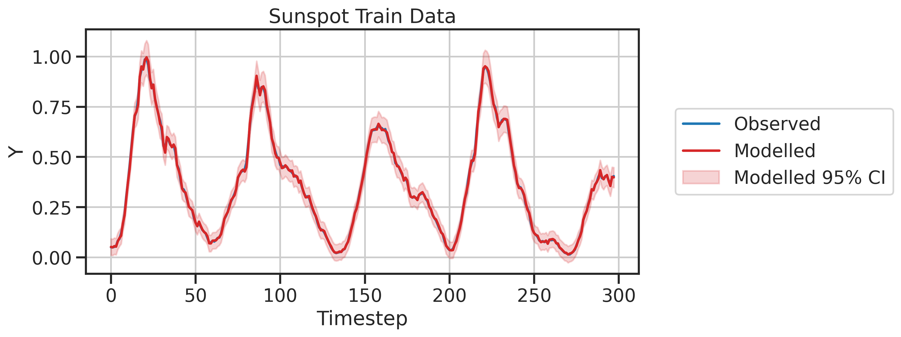
(a) Predictions and actual train dataset for Sunspot

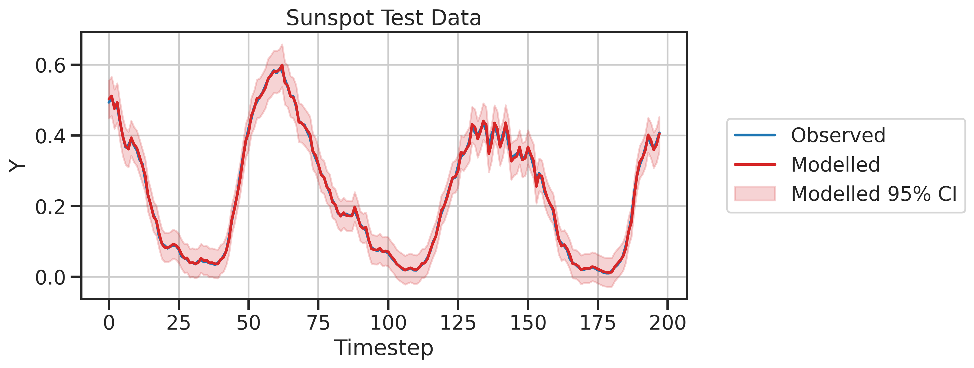
(b) Predictions and actual test dataset for Sunspot

Figure 10: Bayesian linear regression model - Sunspot dataset

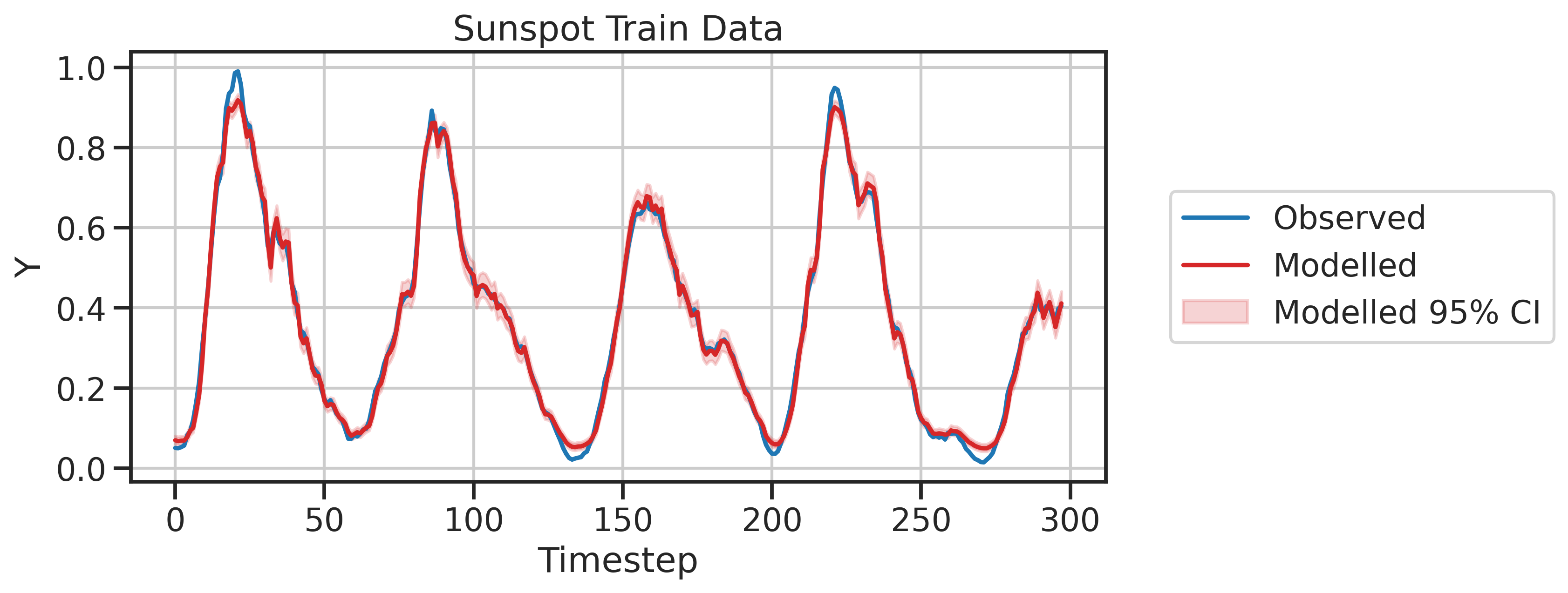
(a) Predictions and actual train dataset for Sunspot

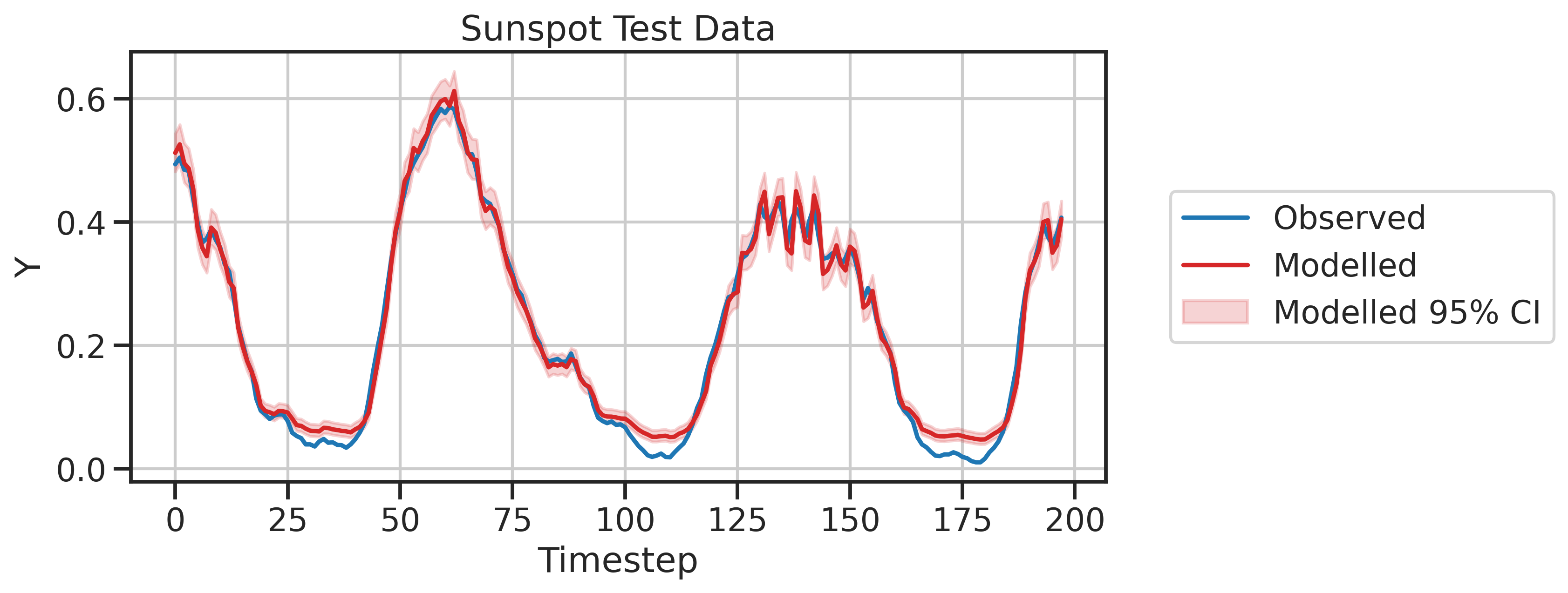
(b) Predictions and actual test dataset for Sunspot

Figure 11: Bayesian neural network model - Sunspot dataset

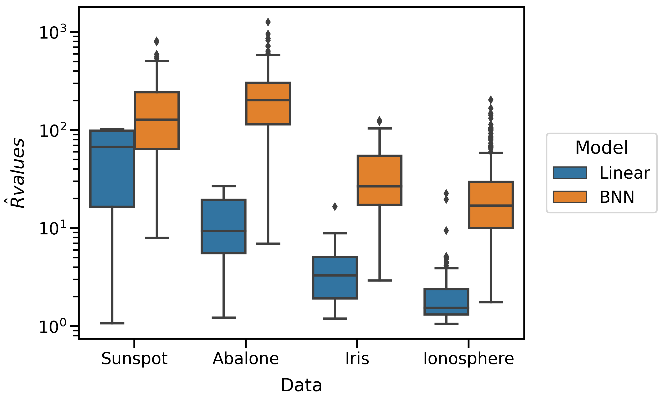
Figure 12: Distribution of $\hat{R}$ values for our Bayesian linear model and Bayesian neural network.

6 Convergence diagnosis

It is important to ensure that the MCMC sampling is adequately exploring the parameter space and constructing an accurate picture of the posterior distribution. One method of monitoring the performance of the adopted MCMC sampler is to examine convergence diagnostic to monitor the extent to which the Markov chains have become a stationary distribution. Practitioners routinely apply the Gelman-Rubin (GR) convergence diagnostic to this end [120]. This diagnostic is developed using sampling from multiple MCMC chains whereby the variance of each chain is assessed independently (within-chain variance) and then compared to the variance between the multiple chains (between-chain variance) for each parameter. Large differences between these two variances would indicate the at the chains have not converged on the same stationary distribution.

For our examples above, we will therefore run a number of independent experiments and compare the MCMC chains using the convergence diagnostic. This measure of convergence is calculated as the potential scale reduction factor (PSRF or $\hat{R}$), where values of PSRF close to 1 indicate convergence. The PSRF is obtained by first calculating the between-chain variance

$$B=\frac{n}{m-1}\sum_{j=1}^{m}(\bar{\theta_{j}}-\bar{\bar{\theta}})^{2}$$ (41)

and within-chain variance

$$W=\frac{1}{m}\sum_{j=1}^{m}s_{j}^{2}$$ (42)

where $n$ is the number of samples, $m$ is the number of chains,

$$\bar{\theta_{j}}=\frac{1}{n}\sum_{i=1}^{n}\theta_{ij}$$

$$\bar{\bar{\theta}}=\frac{1}{m}\sum_{j=1}^{m}\bar{\theta_{j}}$$

and

$$s_{j}^{2}=\frac{1}{n-1}\sum_{j=1}^{n}\theta_{ij}-\bar{\theta_{j}}$$

After observing these estimates, we may then estimate the target variance $\sigma^{2}$ with

$$\hat{\sigma}^{2}=\frac{n-1}{n}W+\frac{B}{n}$$

Then what is known about $\theta$ can be estimated and the result is an approximate Student t’s distribution for $\theta$ with centre $\bar{\bar{\theta}}$, scale $\sqrt{\hat{V}}=\sqrt{\hat{\sigma}^{2}+\frac{B}{mn}}$ and degrees of freedom $d=\frac{2\hat{V}}{\hat{\text{var}}(\hat{V})}$. Here

$$\hat{\text{var}}(\hat{V}) =\left(\frac{n-1}{n}\right)^{2}\frac{1}{m}\hat{\text{var}}(s_{i}^{2})+\left(\frac{m+1}{mn}\right)^{2}\frac{2}{m-1}B^{2}$$

$$+2\frac{(m+1)(n-1)}{mn^{2}}$$

$$\cdot\frac{n}{m}[\hat{\text{cov}}(s_{i}^{2},\bar{\theta_{i}^{2}})-2\bar{\bar{\theta}}\hat{\text{cov}}(s_{i}^{2},\bar{\theta_{i}})].$$

Finally, we calculate the PSRF given by $\hat{R}$ as

$$\sqrt{\hat{R}}=\sqrt{\frac{\hat{V}}{W}\frac{d}{d-2}}$$ (43)

Listing 13 gives further details of the Python implementation .

⬇

1def gelman_rubin(data):

2 """

3 Apply Gelman-Rubin convergence diagnostic to a bunch of chains.

4 :param data: np.array of shape (Nchains, Nsamples, Npars)

5 """

6 Nchains, Nsamples, Npars = data.shape

7 B_on_n = data.mean(axis=1).var(axis=0) # variance of in-chain means

8 W = data.var(axis=1).mean(axis=0) # mean of in-chain variances

9

10 sig2 = (Nsamples/(Nsamples-1))*W + B_on_n

11 Vhat = sig2 + B_on_n/Nchains

12 Rhat = Vhat/W

13

14 # advanced version that accounts for ndof

15 m, n = np.float(Nchains), np.float(Nsamples)

16 si2 = data.var(axis=1)

17 xi_bar = data.mean(axis=1)

18 xi2_bar = data.mean(axis=1)**2

19 var_si2 = data.var(axis=1).var(axis=0)

20 allmean = data.mean(axis=1).mean(axis=0)

21 cov_term1 = np.array([np.cov(si2[:,i], xi2_bar[:,i])[0,1]

22 for i in range(Npars)])

23 cov_term2 = np.array([-2*allmean[i]*(np.cov(si2[:,i], xi_bar[:,i])[0,1])

24 for i in range(Npars)])

25 var_Vhat = ( ((n-1)/n)**2 * 1.0/m * var_si2

26 + ((m+1)/m)**2 * 2.0/(m-1) * B_on_n**2

27 + 2.0*(m+1)*(n-1)/(m*n**2)

28 * n/m * (cov_term1 + cov_term2))

29 df = 2*Vhat**2 / var_Vhat

30 Rhat *= df/(df-2)

31

32 return Rhat

Listing 13: Python implementation Gelman-Rubin diagnostic

6.1 Results

We show results for Gelman-Rubin diagnosis for Bayesian linear regression and Bayesian neural networks using the the Sunspot problem. We test five chains for each model, each with 5,000 samples of weights excluding burn-in samples and evaluating the $\hat{R}$ values for each weight. Figure 12 shows the distribution of the $\hat{R}$ values on a log-scale, and we observe that the $\hat{R}$ values of the weights for Bayesian linear regression model are all much smaller than Bayesian neural network. We can conclude that the Bayesian neural network shows poor convergence based on the Gelman-Rubin diagnostics presented.

By closely examining each weight individually, we observe that the problem of non-convergence mainly arises from multi-modality of the posterior. In Figure 13 we look at samples from a single chain of 25,000 samples excluding 50% burn-in. In Figure 13a and 13b, we present a visualisation for a selected weight from the Bayesian linear model. In Figure 13c and 13d, we present a visualisation for a selected weight from the Bayesian neural network model. We observe potential multi-modal distributions in both cases, with a high degree of auto-correlation and poor convergence. To examine the impact of longer MCMC chains in achieving convergence, an additional test was run taking 400,000 samples excluding 20% burn-in and then thinning the chain by a factor of 50. These thinned results are shown for the Iris dataset in Figure 14. We can see that the chains exhibit more desirable properties and (particularly in the case of the linear model as shown in Figure 14a,b) convergence diagnostics were improved as expected when removing some of the auto-correlation through thinning. We can see in Figure 14c,d that the Bayesian neural network still exhibits a multi-model posterior for this parameter.

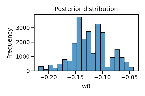
(a) Linear model parameter Posterior

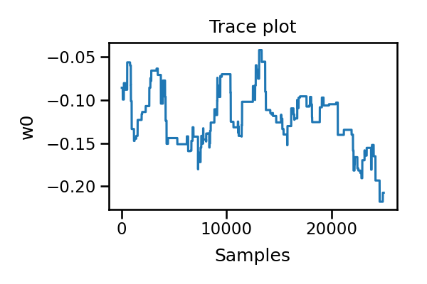
(b) Linear model parameter Trace-plot

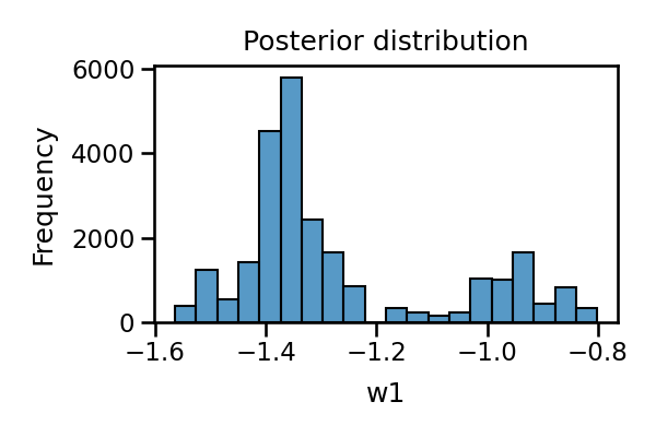
(c) BNN parameter Posterior

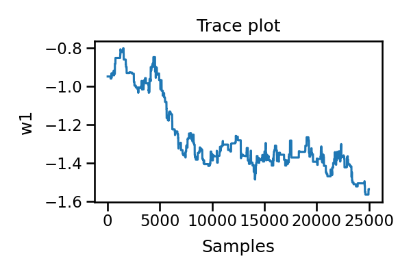
(d) BNN parameter Trace-plot

Figure 13: Posterior and trace-plot for a paramater in each of the Bayesian linear and Bayesian Neural Net models - Sunspot data. For this example, 25,000 samples were taken excluding 20% burn-in with the chain thinned by a factor of 50.

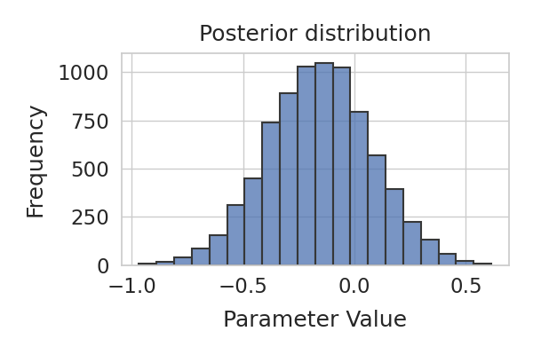
(a) Linear mdoel parameter Posterior

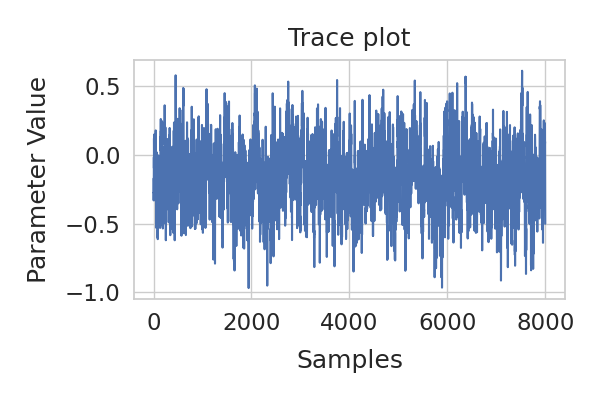
(b) Linear model parameter Trace-plot

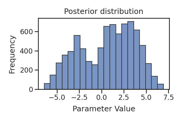
(c) BNN parameter Posterior

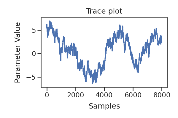
(d) BNN parameter Trace-plot

Figure 14: Posterior and trace-plot for a paramater in each of the Bayesian linear and Bayesian Neural Net models - Iris data. For this example, 400,000 samples were taken excluding 50% burn-in with no thinning.

7 Discussion

Overall, this highlights the problem of applying Gelman-Rubin diagnostics on the weights of Bayesian neural networks. We observe that the Bayesian neural network performs better than the Bayesian linear regression in most prediction problems, despite showing no indications of convergence. This is due to the challenge of attaining MCMC convergence in the weights of Bayesian neural networks, as they are influenced by the problem of multi-modality. Hence, we conclude that for a Bayesian neural network, a poor performance in the Gelman-Rubin diagnostics does not necessarily imply a poor performance in prediction tasks. We revisit the principle of equifinality [121, 122] that states that in open systems, a given end state can be reached by many potential means. In our case, the system is a neural network model and many solutions exist that represent a trained model displaying some level of performance accuracy. Despite this, we note that the goal of Bayesian models are to offer uncertainty quantification in predictions, and proper convergence is required. The original Gelman-Rubin diagnosis [120] motivated a number of enhancements for different types of problems [123, 124, 125]; and we may need to develop better diagnosis for Bayesian neural networks. Nonetheless, in our case comparing Bayesian logistic regression (converged) and Bayesian neural networks (not converged), but achieved good accuracy, we can safely state that so our our Bayesian neural network can only provide a means for uncertainty quantification but is not mature enough to qualify as a robust Bayesian model.

We also revisit convergence issue in the case of Bayesian linear model as shown in Panel (a) - Figure 13, which shows a multi-modal distribution that has not well converged. In the case of linear models, we can have certain features that are not contributing much to the decision making process (predictions) and the weights associated (coefficients) with those features may not converge since they are not really contributing. This is similar to the case of neural networks, where certain weight links are not needed and can be pruned.

We note that we attach much higher acceptance rate in Bayesian neural networks for classification problems (Table 2) when compared to regression problems(Table 2). We note that multinomial likelihood is used for the classification, and Gaussian likelihood is used for the regression problems, and both use Langevin-gradient proposal distributions that account for detailed balanced condition. Hence, we need to fine tune the hyper-parameters associated with the proposal distribution to ensure we get higher acceptance rate for the regression problems. Although 23 % acceptance rate [119] has been prominently used as a ”golden rule”, the optimal acceptance rate depends on the nature of the problem. The number of parameters, Langevin-based proposal distribution, and type of model would raise questions about the established acceptance rate [126]. Hence, more work needs to be done to establish what acceptance rates are appropriate for simple neural networks and deep learning models.

A way to address the issue of convergence would be to develop an ensemble of linear models that can complete with the accuracy of neural networks or deep learning models. In ensemble methods such as bagging and boosting, we can use linear models that have attained convergence as per Gelman-Rubin diagnosis and then combine results of the ensemble using averaging and voting, as done in ensemble methods. Furthermore, we note that Langevin-based MCMC is a way ahead but not the only way ahead. A number of works have utilised the Hamiltonian MCMC which provides another approach to incorporate gradients in MCMC methods that can provide advantages over Langevin-based methods; however, we need comprehensive evaluation studies to check how both methods work for deep learning models such as CNN and LSTM.

Our previous work has shown that despite the challenges, the combination of Langevin-gradients with parallel tempering MCMC [59], presents opportunities for sampling larger neural network architectures [66, 65]. The need to feature a robust methodology for uncertainty quantification in CNNs will make them more suitable for applications where uncertainty in decision making poses major risks, such as medical image analysis [127] and human security [128]. Recently, CNNs have been considered for modelling temporal sequences, they have proven to be successful for time series classification [129, 130], and time series forecasting problems [131, 132]. Our recent work has shown that one dimensional CNNs provide better prediction performance than LSTM-based models for multi-step time series prediction problems [133]. Leveraging CNNs within a Bayesian framework can provide better uncertainty quantification in predictions and make them useful for cutting-edge real-world applications.

We envision that this tutorial will enable statisticians and machine learners to utilise MCMC sampling in a more effective way when developing new models and also developing a Bayesian framework for existing deep learning models. The tutorial has introduced basic concepts with code and provides an overview of challenges, when it comes to convergence of Bayesian neural networks.

8 Code and Data

All code (for implementation, results and figures) and data presented in this paper are available in the associated github repository. This repository presents the implementations in separate Jupyter notebooks in the base directory, with sub-directories containing data, convenient functions and details of the environment setup.

References

- [1] G. E. Box, G. C. Tiao, Bayesian inference in statistical analysis, Vol. 40, John Wiley & Sons, 2011.
- [2] G. Chamberlain, G. W. Imbens, Nonparametric applications of bayesian inference, Journal of Business & Economic Statistics 21 (1) (2003) 12–18.
- [3] J. Geweke, Bayesian inference in econometric models using monte carlo integration, Econometrica: Journal of the Econometric Society (1989) 1317–1339.
- [4] R. Chandra, R. D. Müller, D. Azam, R. Deo, N. Butterworth, T. Salles, S. Cripps, Multicore parallel tempering Bayeslands for basin and landscape evolution, Geochemistry, Geophysics, Geosystems 20 (11) (2019) 5082–5104.
- [5] J. Pall, R. Chandra, D. Azam, T. Salles, J. M. Webster, R. Scalzo, S. Cripps, Bayesreef: A bayesian inference framework for modelling reef growth in response to environmental change and biological dynamics, Environmental Modelling & Software (2020) 104610.
- [6] D. P. Kingma, J. Ba, Adam: A method for stochastic optimization, arXiv preprint arXiv:1412.6980 (2014).
- [7] D. J. MacKay, Probable networks and plausible predictions—a review of practical bayesian methods for supervised neural networks, Network: Computation in Neural Systems 6 (3) (1995) 469–505.
- [8] R. M. Neal, Bayesian learning for neural networks, Vol. 118, Springer Science & Business Media, 2012.
- [9] D. F. Specht, Probabilistic neural networks, Neural networks 3 (1) (1990) 109–118.
- [10] M. D. Richard, R. P. Lippmann, Neural network classifiers estimate bayesian a posteriori probabilities, Neural computation 3 (4) (1991) 461–483.
- [11] E. A. Wan, Neural network classification: A bayesian interpretation, IEEE Transactions on Neural Networks 1 (4) (1990) 303–305.
- [12] Z. Ghahramani, Probabilistic machine learning and artificial intelligence, Nature 521 (7553) (2015) 452–459.
- [13] S. Chib, E. Greenberg, Understanding the Metropolis-Hastings algorithm, The american statistician 49 (4) (1995) 327–335.
- [14] C. P. Robert, G. Casella, The Metropolis—Hastings algorithm, in: Monte Carlo statistical methods, Springer, 1999, pp. 231–283.
- [15] D. B. Hitchcock, A history of the Metropolis–Hastings algorithm, The American Statistician 57 (4) (2003) 254–257.
- [16] G. Casella, E. I. George, Explaining the Gibbs sampler, The American Statistician 46 (3) (1992) 167–174.
- [17] C. K. Carter, R. Kohn, On Gibbs sampling for state space models, Biometrika 81 (3) (1994) 541–553.
- [18] G. O. Roberts, A. F. Smith, Simple conditions for the convergence of the Gibbs sampler and Metropolis-Hastings algorithms, Stochastic processes and their applications 49 (2) (1994) 207–216.
- [19] P. J. Rossky, J. D. Doll, H. L. Friedman, Brownian dynamics as smart Monte Carlo simulation, The Journal of Chemical Physics 69 (10) (1978) 4628–4633.
- [20] G. O. Roberts, R. L. Tweedie, Exponential convergence of langevin distributions and their discrete approximations, Bernoulli (1996) 341–363.
- [21] G. O. Roberts, J. S. Rosenthal, Optimal scaling of discrete approximations to langevin diffusions, Journal of the Royal Statistical Society: Series B (Statistical Methodology) 60 (1) (1998) 255–268.
- [22] B. D. Flury, Acceptance–rejection sampling made easy, Siam Review 32 (3) (1990) 474–476.
- [23] W. R. Gilks, P. Wild, Adaptive rejection sampling for Gibbs sampling, Journal of the Royal Statistical Society: Series C (Applied Statistics) 41 (2) (1992) 337–348.
- [24] A. Brockwell, P. Del Moral, A. Doucet, Sequentially interacting Markov chain Monte Carlo methods, The Annals of Statistics (2010) 3387–3411.
- [25] C. Andrieu, J. Thoms, A tutorial on adaptive MCMC, Statistics and computing 18 (4) (2008) 343–373.
- [26] R. H. Swendsen, J.-S. Wang, Replica monte carlo simulation of spin-glasses, Physical review letters 57 (21) (1986) 2607.
- [27] K. Hukushima, K. Nemoto, Exchange monte carlo method and application to spin glass simulations, Journal of the Physical Society of Japan 65 (6) (1996) 1604–1608.
- [28] D. J. Earl, M. W. Deem, Parallel tempering: Theory, applications, and new perspectives, Physical Chemistry Chemical Physics 7 (23) (2005) 3910–3916.
- [29] M. Sambridge, A parallel tempering algorithm for probabilistic sampling and multimodal optimization, Geophysical Journal International 196 (1) (2014) 357–374.
- [30] Y. Fan, S. A. Sisson, Reversible jump MCMC, Handbook of Markov Chain Monte Carlo (2011) 67–92.
- [31] S. P. Brooks, P. Giudici, G. O. Roberts, Efficient construction of reversible jump Markov chain Monte Carlo proposal distributions, Journal of the Royal Statistical Society: Series B (Statistical Methodology) 65 (1) (2003) 3–39.
- [32] C. Tarantola, Mcmc model determination for discrete graphical models, Statistical Modelling 4 (1) (2004) 39–61.
- [33] F. Liang, C. Liu, Efficient MCMC estimation of discrete distributions, Computational statistics & data analysis 49 (4) (2005) 1039–1052.
- [34] G. Zanella, Informed proposals for local mcmc in discrete spaces, Journal of the American Statistical Association 115 (530) (2020) 852–865.
- [35] W. J. Browne, MCMC algorithms for constrained variance matrices, Computational Statistics & Data Analysis 50 (7) (2006) 1655–1677.
- [36] A. R. Gallant, H. Hong, M. P. Leung, J. Li, Constrained estimation using penalization and MCMC, Journal of Econometrics 228 (1) (2022) 85–106.
- [37] S. A. Sisson, Y. Fan, Likelihood-free MCMC, Chapman & Hall/CRC, New York.[839], 2011.
- [38] D. A. Van Dyk, X.-L. Meng, The art of data augmentation, Journal of Computational and Graphical Statistics 10 (1) (2001) 1–50.
- [39] L. L. Duan, J. E. Johndrow, D. B. Dunson, Scaling up data augmentation MCMC via calibration, The Journal of Machine Learning Research 19 (1) (2018) 2575–2608.
- [40] J. Zobitz, A. Desai, D. Moore, M. Chadwick, A primer for data assimilation with ecological models using Markov Chain Monte Carlo (MCMC), Oecologia 167 (3) (2011) 599–611.
- [41] C. Andrieu, P. Djurić, A. Doucet, Model selection by MCMC computation, Signal Processing 81 (1) (2001) 19–37.
- [42] C. Andrieu, A. Doucet, Joint Bayesian model selection and estimation of noisy sinusoids via reversible jump MCMC, IEEE Transactions on Signal Processing 47 (10) (1999) 2667–2676.
- [43] A. S. Mugglin, B. P. Carlin, L. Zhu, E. Conlon, Bayesian areal interpolation, estimation, and smoothing: an inferential approach for geographic information systems, Environment and Planning A 31 (8) (1999) 1337–1352.
- [44] M. Sambridge, Geophysical inversion with a neighbourhood algorithm—ii. appraising the ensemble, Geophysical Journal International 138 (3) (1999) 727–746.
- [45] M. Sambridge, K. Mosegaard, Monte carlo methods in geophysical inverse problems, Reviews of Geophysics 40 (3) (2002).
- [46] R. Scalzo, D. Kohn, H. Olierook, G. Houseman, R. Chandra, M. Girolami, S. Cripps, Efficiency and robustness in Monte Carlo sampling for 3-D geophysical inversions with Obsidian v0. 1.2: Setting up for success, Geoscientific Model Development 12 (7) (2019) 2941–2960.
- [47] R. Chandra, D. Azam, R. D. Müller, T. Salles, S. Cripps, Bayeslands: A Bayesian inference approach for parameter uncertainty quantification in badlands, Computers & Geosciences 131 (2019) 89–101.
- [48] H. K. Olierook, R. Scalzo, D. Kohn, R. Chandra, E. Farahbakhsh, C. Clark, S. M. Reddy, R. D. Müller, Bayesian geological and geophysical data fusion for the construction and uncertainty quantification of 3D geological models, Geoscience Frontiers 12 (1) (2021) 479–493.
- [49] L. Marshall, D. Nott, A. Sharma, A comparative study of Markov chain Monte Carlo methods for conceptual rainfall-runoff modeling, Water Resources Research 40 (2) (2004).
- [50] J. A. Vrugt, C. J. Ter Braak, M. P. Clark, J. M. Hyman, B. A. Robinson, Treatment of input uncertainty in hydrologic modeling: Doing hydrology backward with Markov chain Monte Carlo simulation, Water Resources Research 44 (12) (2008).
- [51] G. I. Valderrama-Bahamóndez, H. Fröhlich, MCMC techniques for parameter estimation of ODE based models in systems biology, Frontiers in Applied Mathematics and Statistics 5 (2019) 55.
- [52] Y. Nishiyama, Y. Saikawa, N. Nishiyama, Interaction between the immune system and acute myeloid leukemia: A model incorporating promotion of regulatory T cell expansion by leukemic cells, Biosystems 165 (2018) 99–105.
- [53] B. Rannala, Identifiability of parameters in MCMC Bayesian inference of phylogeny, Systematic biology 51 (5) (2002) 754–760.
- [54] D. Sorensen, D. Gianola, D. Gianola, Likelihood, Bayesian and MCMC methods in quantitative genetics (2002).
- [55] A. J. Drummond, M. A. Suchard, D. Xie, A. Rambaut, Bayesian phylogenetics with beauti and the beast 1.7, Molecular biology and evolution 29 (8) (2012) 1969–1973.
- [56] M. Girolami, B. Calderhead, Riemann manifold langevin and hamiltonian monte carlo methods, Journal of the Royal Statistical Society: Series B (Statistical Methodology) 73 (2) (2011) 123–214.
- [57] R. M. Neal, et al., Mcmc using hamiltonian dynamics, Handbook of Markov Chain Monte Carlo 2 (11) (2011).
- [58] M. Welling, Y. W. Teh, Bayesian learning via stochastic gradient langevin dynamics, in: Proceedings of the 28th International Conference on Machine Learning (ICML-11), 2011, pp. 681–688.
- [59] R. Chandra, K. Jain, R. V. Deo, S. Cripps, Langevin-gradient parallel tempering for bayesian neural learning, Neurocomputing 359 (2019) 315 – 326.
- [60] M. M. Drugan, D. Thierens, Evolutionary Markov chain Monte Carlo, in: International Conference on Artificial Evolution (Evolution Artificielle), Springer, 2004, pp. 63–76.
- [61] C. J. Ter Braak, A Markov Chain Monte Carlo version of the genetic algorithm differential evolution: easy Bayesian computing for real parameter spaces, Statistics and Computing 16 (3) (2006) 239–249.
- [62] C. J. Ter Braak, J. A. Vrugt, Differential evolution markov chain with snooker updater and fewer chains, Statistics and Computing 18 (4) (2008) 435–446.
- [63] A. Kapoor, E. Nukala, R. Chandra, Bayesian neuroevolution using distributed swarm optimization and tempered MCMC, Applied Soft Computing 129 (2022) 109528.
- [64] L. Bottou, Large-scale machine learning with stochastic gradient descent, in: Proceedings of COMPSTAT’2010, Springer, 2010, pp. 177–186.
- [65] R. Chandra, M. Jain, M. Maharana, P. N. Krivitsky, Revisiting Bayesian autoencoders with MCMC, IEEE Access 10 (2022) 40482–40495.
- [66] R. Chandra, A. Bhagat, M. Maharana, P. N. Krivitsky, Bayesian graph convolutional neural networks via tempered MCMC, IEEE Access 9 (2021) 130353–130365.
- [67] L. Li, A. Holbrook, B. Shahbaba, P. Baldi, Neural network gradient hamiltonian monte carlo, Computational statistics 34 (1) (2019) 281–299.
- [68] D. M. Blei, A. Kucukelbir, J. D. McAuliffe, Variational inference: A review for statisticians, Journal of the American Statistical Association 112 (518) (2017) 859–877.
- [69] A. Graves, Practical variational inference for neural networks, in: Advances in Neural Information Processing Systems 24, 2011, pp. 2348–2356.
- [70] C. Blundell, J. Cornebise, K. Kavukcuoglu, D. Wierstra, Weight uncertainty in neural network, in: Proceedings of The 32nd International Conference on Machine Learning, 2015, pp. 1613–1622.
- [71] N. Srivastava, G. Hinton, A. Krizhevsky, I. Sutskever, R. Salakhutdinov, Dropout: A simple way to prevent neural networks from overfitting, The Journal of Machine Learning Research 15 (1) (2014) 1929–1958.
- [72] Y. Gal, Z. Ghahramani, Dropout as a bayesian approximation: Representing model uncertainty in deep learning, in: international conference on machine learning, 2016, pp. 1050–1059.
- [73] K. Shridhar, F. Laumann, M. Liwicki, A comprehensive guide to bayesian convolutional neural network with variational inference (2019). arXiv:1901.02731.
- [74] Y. Gal, Z. Ghahramani, A theoretically grounded application of dropout in recurrent neural networks, Advances in neural information processing systems 29 (2016).
- [75] J. M. Bernardo, A. F. Smith, Bayesian theory, Vol. 405, John Wiley & Sons, 2009.
- [76] G. A. Barnard, T. Bayes, Studies in the history of probability and statistics: IX. Thomas Bayes’s essay towards solving a problem in the doctrine of chances, Biometrika 45 (3/4) (1958) 293–315.
- [77] A. I. Dale, A history of inverse probability: From Thomas Bayes to Karl Pearson, Springer Science & Business Media, 2012.
- [78] P. S. Laplace, Memoir on the probability of the causes of events, Statistical science 1 (3) (1986) 364–378.
- [79] S. R. Johnson, G. A. Tomlinson, G. A. Hawker, J. T. Granton, B. M. Feldman, Methods to elicit beliefs for Bayesian priors: a systematic review, Journal of clinical epidemiology 63 (4) (2010) 355–369.
- [80] K. M. Banner, K. M. Irvine, T. J. Rodhouse, The use of Bayesian priors in ecology: The good, the bad and the not great, Methods in Ecology and Evolution 11 (8) (2020) 882–889.
- [81] R. van de Schoot, S. Depaoli, R. King, B. Kramer, K. Märtens, M. G. Tadesse, M. Vannucci, A. Gelman, D. Veen, J. Willemsen, et al., Bayesian statistics and modelling, Nature Reviews Methods Primers 1 (1) (2021) 1–26.
- [82] W. Li, G. Lin, An adaptive importance sampling algorithm for bayesian inversion with multimodal distributions, Journal of Computational Physics 294 (2015) 173–190.
- [83] S. Hu, D. S. Poskitt, X. Zhang, Bayesian adaptive bandwidth kernel density estimation of irregular multivariate distributions, Computational Statistics & Data Analysis 56 (3) (2012) 732–740.
- [84] R. Rojas, A short proof of the posterior probability property of classifier neural networks, Neural Computation 8 (1) (1996) 41–43.
- [85] H. Akaike, Likelihood and the bayes procedure, in: Selected Papers of Hirotugu Akaike, Springer, 1998, pp. 309–332.
- [86] D. J. MacKay, Hyperparameters: Optimize, or integrate out?, in: Maximum entropy and Bayesian methods, Springer, 1996, pp. 43–59.
-
[87]
A. Gelman, J. B. Carlin, H. S. Stern, D. B. Rubin,