Borel resummation of secular divergences in stochastic inflation

Abstract

We make use of Borel resummation to extract the exact time dependence from the divergent series found in the context of stochastic inflation. Correlation functions of self-interacting scalar fields in de Sitter spacetime are known to develop secular IR divergences via loops, and the first terms of the divergent series have been consistently computed both with standard techniques for curved spacetime quantum field theory and within the framework of stochastic inflation. We show that Borel resummation can be used to interpret the divergent series and to correctly infer the time evolution of the correlation functions. In practice, we adopt a method called Borel–Padé resummation where we approximate the Borel transformation by a Padé approximant. We also discuss the singularity structures of Borel transformations and mention possible applications to cosmology.

YITP-23-43, RIKEN-iTHEMS-Report-23, RESCEU-7/23

1 Introduction

Cosmic inflation, an era of quasi de Sitter expansion of the early Universe, is now the leading paradigm to describe the earliest cosmological history. In addition to solving the horizon and flatness problems of the standard hot Big Bang model 10.1093/mnras/195.3.467 ; PhysRevD.23.347 ; Starobinsky:1980te ; Linde:1981mu ; PhysRevLett.48.1220 ; Linde:1983gd , inflation provides an explanation for the origin of structures in our Universe. Vacuum fluctuations are generated deep inside the horizon and then stretched to cosmological scales by the accelerated expansion, thus seeding Cosmic Microwave Background (CMB) anisotropies and the Large-Scale Structure (LSS). The simplest model of inflation, a slowly-rolling scalar field, predicts nearly scale-invariant, adiabatic, and sufficiently small cosmological scalar fluctuations, being consistent with the current large-scale observations Planck2018VI ; Planck2018X .

Although the physics of inflation is rather constrained at the largest cosmological scales emerging from vacuum fluctuations during an epoch deep inside the inflationary era, much remains to be understood about the remaining of the inflationary evolution through small-scale observations. For example, if fluctuations at small cosmological scales are sufficiently enhanced compared to those at the CMB ones, a significant amount of primordial black holes (PBHs) could be produced when primordial perturbations re-enter the Hubble horizon in the radiation- and matter-dominated eras 1967SvA….10..602Z ; 10.1093/mnras/152.1.75 ; 10.1093/mnras/168.2.399 ; 1975ApJ…201….1C . In those scenarios, it may happen that fluctuations at small scales are so large that standard perturbation theory breaks down and that one needs a non-perturbative formalism to describe them. Stochastic inflation Starobinsky:1986fx precisely enables one to treat such large fluctuations in a non-perturbative way, and correctly infer the statistical properties of primordial fluctuations in this regime. Actually, it is now believed that the formation of primordial black holes is mostly sensitive to very large over-densities, rather than an overall increase of the root mean square density. These rare events, located in the tails of the distribution of fluctuations, cannot be described by the usual perturbation theory, even without an amplification mechanism at a specific scale. For example, the stochastic formalism has been used to prove that exponential tails can typically develop away from the center of the distribution, potentially leading to many more primordial black holes than a Gaussian distribution with the same power spectrum Pattison_2017 ; Pattison_2021 ; Vennin:2020kng ; Ezquiaga_2020 ; PhysRevLett.127.101302 ; Achucarro:2021pdh . Other than their implication in terms of primordial black holes, small-scale amplification mechanisms are also investigated for their potential to lead to secondary gravitational waves at horizon re-entry (see Domenech:2021ztg for a recent review), as well as to spectral distortions in the CMB at intermediates scales (see, e.g. Kogut:2019vqh for a recent update on the status and prospects of these observables).

In the stochastic inflation framework (see the seminal works STAROBINSKY1982175 ; Starobinsky:1986fx ; NAMBU1988441 ; NAMBU1989240 ; Kandrup:1988sc ; Nakao:1988yi ; Nambu:1989uf ; Mollerach:1990zf ; Linde:1993xx ; Starobinsky:1994bd ), the long-wavelength modes of the scalar field are driven by an effectively classical, yet stochastic dynamics. The source of the stochasticity stems from the quantum nature of the vacuum fluctuations of this bosonic field. When these microphysical fluctuations are stretched on super-Hubble scales, they join the infrared sector of the scalar field. One can therefore see the coarse-grained, long-wavelength modes, as an open system subject to a constant interaction with a bath of ultra-violet modes. This interaction is most notably described as a noise term in a stochastic differential equation for the infrared system, called a Langevin equation. Correspondingly, from the Langevin equation (and given a time discretisation scheme), one can consider the associated Fokker–Planck equation for the probability density function (PDF) of coarse-grained modes. Although the dynamics may be exactly solvable for some classes of systems, it is in general difficult to obtain the full behaviour without numerical calculations. However, important analytical results have been derived with the stochastic formalism, at least in three directions.

• The first one, which is also the main focus of this work, is the series expansion of the field’s correlation functions in terms of $\log a$, where $a$ is the scale factor. Excellent agreement has been shown between the stochastic approach and various quantum field theory techniques, mostly in the paradigmatic setup of $\lambda\phi^{4}$ theory, for the first orders of the series expansion Starobinsky:1994bd ; Prokopec:2007ak ; Finelli:2008zg ; Finelli:2010sh ; Garbrecht:2013coa ; Garbrecht:2014dca ; Onemli:2015pma ; Cho:2015pwa (see also Pinol:2018euk ; Pinol:2020cdp for the first such predictions in the context of multifield stochastic inflation with curved field space). As these time series are divergent, an effect known as secular divergences, the expansion is reputed trustworthy at early times only; in this work we precisely revisit this question and extend the validity of these results up to sufficiently late time.

• The second direction concerns the opposite, late-time expansion of the correlation functions and the related PDF. These results (see, e.g. Seery:2007we ; Enqvist:2008kt ; 2009JCAP…05..021S ; Burgess:2009bs ; Seery:2010kh ; Gautier:2013aoa ; Guilleux:2015pma ; Gautier:2015pca ; Hardwick:2017fjo ; Markkanen:2017rvi ; LopezNacir:2019ord ; Gorbenko:2019rza ; Mirbabayi:2019qtx ; Adshead:2020ijf ; Moreau:2020gib ; Cohen:2020php ), are impressive as they somehow encompass the late-time resummation of the IR secular divergences previously mentioned.

• A third direction, more directly related to cosmology and inflation, concerns the application of the stochastic formalism to the derivation of primordial correlation functions for the curvature perturbation. The so-called stochastic $\delta N$-formalism, enables one to derive those statistics from the fluctuations of the duration of inflation in uncorrelated patches of the universe Salopek:1990jq ; Sasaki:1995aw ; Sasaki:1998ug ; Lyth:2004gb ; Fujita:2013cna ; Fujita:2014tja ; Vennin:2015hra ; Kawasaki:2015ppx ; Assadullahi:2016gkk ; Vennin:2016wnk , proving notably useful for predicting the abundance of primordial black holes Kawasaki:2015ppx ; Pattison:2017mbe ; Ezquiaga:2018gbw ; Biagetti:2018pjj ; Ezquiaga:2019ftu ; Panagopoulos:2019ail ; Achucarro:2021pdh .

In this work, we bridge the gap between the early- and late-time expansions of the stochastic formalism (the first and second points), by providing a way to resum the IR secular divergences at any finite of infinite time,

Borel resummation ASENS_1899_3_16__9_0 is one of the standard methods to resum formally divergent series. It not only makes sense out of divergent series, but also gives us information on non-perturbative effects through analytic structures in the Borel plane via resurgence relations SC_1977__17_1_A5_0 . While Borel resummation and resurgence have long history of applications to quantum mechanics Bender:1969si ; Bender:1973rz ; Balian:1978et ; AIHPA_1983__39_3_211_0 ; ZinnJustin:2004ib ; ZinnJustin:2004cg ; Jentschura:2010zza ; Jentschura:2011zza ; Dunne:2013ada ; Basar:2013eka ; Dunne:2014bca ; Escobar-Ruiz:2015nsa ; Escobar-Ruiz:2015rfa ; Misumi:2015dua ; Behtash:2015zha ; Behtash:2015loa ; Gahramanov:2015yxk ; Dunne:2016qix ; Kozcaz:2016wvy ; Fujimori:2016ljw ; Dunne:2016jsr ; Serone:2016qog ; Basar:2017hpr ; Alvarez:2017sza ; Behtash:2018voa ; Duan:2018dvj ; Raman:2020sgw ; Sueishi:2019xcj ; Sueishi:2020rug ; Sueishi:2021xti , currently there are many applications to various other physics such as quantum field theory (QFT), hydrodynamics Aniceto:2015mto ; Basar:2015ava ; Casalderrey-Solana:2017zyh ; Behtash:2017wqg ; Heller:2018qvh ; Heller:2020uuy ; Aniceto:2018uik ; Behtash:2020vqk and string theory Marino:2008vx ; Garoufalidis:2010ya ; Chan:2010rw ; Chan:2011dx ; Schiappa:2013opa ; Marino:2006hs ; Marino:2007te ; Marino:2008ya ; Pasquetti:2009jg ; Aniceto:2011nu ; Santamaria:2013rua ; Couso-Santamaria:2014iia ; Grassi:2014cla ; Couso-Santamaria:2015wga ; Couso-Santamaria:2016vcc ; Couso-Santamaria:2016vwq ; Kuroki:2019ets ; Kuroki:2020rgg ; Dorigoni:2020oon . In particular, QFT recently has a variety of applications of Borel resummation and resurgence, including 2d QFTs Dunne:2012ae ; Dunne:2012zk ; Cherman:2013yfa ; Cherman:2014ofa ; Misumi:2014jua ; Nitta:2014vpa ; Nitta:2015tua ; Behtash:2015kna ; Dunne:2015ywa ; Buividovich:2015oju ; Demulder:2016mja ; Sulejmanpasic:2016llc ; Okuyama:2018clk ; Abbott:2020qnl ; Abbott:2020mba ; Ishikawa:2019tnw ; Ishikawa:2020eht , the Chern-Simons theory Gukov:2016njj ; Gang:2017hbs ; Wu:2020dhl ; Fuji:2020ltq ; Ferrari:2020avq ; Gukov:2019mnk ; Garoufalidis:2020nut , 4d non-supersymmetric QFTs Argyres:2012vv ; Dunne:2015eoa ; Yamazaki:2017ulc ; Mera:2018qte ; Itou:2018wkm ; Canfora:2018clt ; Ashie:2019cmy ; Ishikawa:2019oga ; Unsal:2020yeh ; Ashie:2020bvw ; Morikawa:2020agf , and supersymmetric gauge theories in diverse dimensions Russo:2012kj ; Aniceto:2014hoa ; Aniceto:2015rua ; Honda:2016mvg ; Honda:2016vmv ; Gukov:2016tnp ; Honda:2017qdb ; Gukov:2017kmk ; Dorigoni:2017smz ; Honda:2017cnz ; Fujimori:2018nvz ; Grassi:2019coc ; Dorigoni:2019kux ; Dorigoni:2021guq ; Fujimori:2021oqg . However, there are only few applications so far in the cosmological or astrophysical contexts, and mainly for quasi-normal modes of a black hole Hatsuda:2021gtn ; Hatsuda:2019eoj ; Matyjasek:2019eeu ; Eniceicu:2019npi . The aim of the present paper is to present a new cosmological application of Borel resummation; from a truncated series at some finite order, we reconstruct the long-time evolution of the correlation function from transient to equilibrium regimes. To make the setup as simple as possible, we mainly restrict ourselves to a spectator field in a quartic potential. In order to make contrast with exactly solvable systems, we also discuss a spectator in a quadratic potential in a parallel way.

The organization of the paper is as follows. In Sec. 2, we review the framework of stochastic inflation, focusing on the distribution and correlation functions of a test (spectator) scalar field in the presence of a quadratic or a quartic potential. There we perform a perturbative expansion of the correlation functions and see how it leads to a divergent behaviour in the $\lambda\phi^{4}$ theory. In Sec. 3 we introduce Padé approximants and Borel resummation to recover the correct behaviour of the correlation functions in time. In the application of the Borel resummation, we specifically use a method called Borel–Padé resummation where we approximate Borel transformation (rather than the correlation functions themselves) by the Padé approximant. Section 4 is devoted to discussion and conclusions. In Appendix A, we discuss technicalities of the Borel–Padé resummation technique.

2 Stochastic spectator, its PDF, and the Fokker–Planck equation

The stochastic formalism for inflation Starobinsky:1986fx aims at dealing directly with the super-Hubble part of the quantum fields present during inflation. It is derived as an effective field theory for the long-wavelength modes of scalar fields, after the short-wavelength modes have been integrated out. The quantum properties of these small-scales degrees of freedom are imprinted in the statistical properties of a stochastic noise. This noise then acts as a driving force on the effectively classical dynamics of the so-called coarse-grained fields on super-Hubble scales (see, e.g. Refs. Polarski:1995jg ; Lesgourgues:1996jc ; Polarski:2001yn ; Kiefer:2008ku ; Burgess:2014eoa ; Martin:2015qta , about the quantum-to-classical transition during inflation). The resulting Langevin equations can then be translated into the Fokker–Planck equation, which describes the convection-diffusion of the probability distribution function for the coarse-grained fields. The convection term is given by the usual background dynamics of the fields, and is often dictated by the derivative of a scalar potential (see also Refs. Pinol:2018euk ; Pinol:2020cdp for the incorporation of non-minimal kinetic couplings between scalar fields in the context of stochastic inflation). The diffusion term comes from the noise in the Langevin equation and describes the effect of the small-scale quantum modes crossing the cut-off scale and joining the open system made of super-Hubble fields. In the following, in order to keep the discussion simple, we adopt the simpler approach of stochastic inflation from the point of view of the equations of motion. The stochastic formalism can also be found from the theoretically robust path integral derivation, see Refs. Morikawa:1989xz ; Calzetta:1999zr ; Matarrese:2003ye ; Levasseur:2013ffa ; Moss:2016uix ; Tokuda:2017fdh ; Prokopec:2017vxx ; Pinol:2020cdp .

Throughout this paper, we consider the dynamics of a spectator field $\phi$ during inflation. In practice, we will work at leading order in the slow-roll parameters, which amounts to approximating the quasi-de Sitter background as an exact de Sitter one with a constant Hubble parameter $H=\dot{a}/a$, maintained by another scalar field playing the role of the inflaton. Here, a dot means a derivative with respect to the cosmic time $t$, and $a=a(t)$ is the scale factor with exponential time-dependence. In the following, rather than the cosmic time, we will use the convenient and deterministic (see Ref. Finelli:2008zg ) variable $N=\log a$ called the number of $e$-folds, as a time variable. We decompose the scalar field $\phi$ into UV modes ($\phi_{>}$ for $k>k_{\sigma}(N)$) and IR ones ($\phi_{<}$ for $k<k_{\sigma}(N)$), as

$$\phi(N,{\bf\it x})=\underbrace{\int\frac{\differential^{3}k}{(2\pi)^{3}}\,\Theta(k-k_{\sigma}(N))\tilde{\phi}(N,{\bf\it k})e^{i{\bf\it k}\cdot{\bf\it x}}}_{\equiv\phi_{>}(N,{\bf\it x})}+\underbrace{\int\frac{\differential^{3}k}{(2\pi)^{3}}\,\Theta(-k+k_{\sigma}(N))\tilde{\phi}(N,{\bf\it k})e^{i{\bf\it k}\cdot{\bf\it x}}}_{\equiv\phi_{<}(N,{\bf\it x})}\,\,.$$ (2.1)

We introduced a time-dependent cut-off $k_{\sigma}(N)\equiv\sigma a(N)H$, with $\sigma\ll 1$ a bookkeeping parameter representing the ratio between the physical size of the Hubble radius and the cut-off length. Physically, it is chosen such that modes with wavelength larger than the cut-off scale can be well approximated as classical random variables, rather than fully quantum operators. The fact that the cut-off is time dependent is crucial as time derivatives of the full field $\phi$ will also hit the window function $\Theta$, giving rise to terms absent in the corresponding deterministic, background theory (for which $k_{\sigma}(N)\rightarrow 0$). Here we also defined $\Theta$ as the Heaviside step function, which amounts to a hard cut-off separating the UV sector from the IR one. The choice of the window function is not irrelevant, as our choice of a hard cut-off will result in a white noise, while a smooth window function would have resulted in a colored noise with different statistical properties, see Winitzki:1999ve ; Matarrese:2003ye ; Liguori:2004fa .

The dynamics of the full field $\phi$, before the decomposition into IR and UV modes, is described by the Klein-Gordon equation

$$\partialderivative[2]{\phi}{N}+3\partialderivative{\phi}{N}-\frac{\gradient^{2}\phi}{a^{2}H^{2}}+\frac{1}{H^{2}}\derivative{V}{\phi}=0\,\,,$$ (2.2)

where $V=V(\phi)$ is the scalar potential. Inserting the decomposition (2.1) into Eq. (2.2), and assuming that the quantum fluctuations $\phi_{>}$ behave as in the usual linear perturbation theory, one finds the Langevin equation for the coarse-grained fields:

$$\partialderivative{\phi}{N}=-\frac{1}{3H^{2}}\derivative{V}{\phi}+\xi\,\,.$$ (2.3)

Here and in the following we simply write the long-wavelength field $\phi_{<}$ as $\phi$ since the stochastic formalism gives an effective description of $\phi_{<}$ only. We have also assumed an overdamped approximation for the dyamics of the IR fields, that is that the acceleration term is negligible compared to the other ones. This approximation is well motivated in situations where the scalar field is (at the classical, deterministic level), slowly rolling down the slope of its potential (see Nakao:1988yi ; Habib:1992ci for the first works on stochastic inflation beyond slow roll). The first term in the right hand side of Eq. (2.3) describes the effect of the classical drift, while the second is the classical noise of quantum micro-physical origin, with correlation properties

$$\expectationvalue{\xi(N,{\bf\it x})\xi(N^{\prime},{\bf\it x}^{\prime})}=\frac{H^{2}}{4\pi^{2}}\,\mathrm{sinc}(k_{\sigma}r)\,\delta_{\mathrm{D}}(N-N^{\prime})\,\,.$$ (2.4)

Here $r\equiv\absolutevalue{{\bf\it x}-{\bf\it x}^{\prime}}$ is the comoving distance between the two points. In the following, we will be interested only in the one-point statistics of the fields, and therefore focus effectively on $r=0$ (and therefore $\mathrm{sinc}(k_{\sigma}r)\rightarrow 1$), although in practice our results will be more generally valid for any two points within a patch of the early universe with comoving size $r<k_{\sigma}^{-1}$. We can interpret the presence of the Dirac $\delta$-distribution in time, $\delta_{\mathrm{D}}(N-N^{\prime})$, as the fact that the stochastic dynamics is derived from a white noise. The amplitude of the noise corresponds in general to the power spectrum of the quantum fluctuations $\phi_{>}$ when they cross the cut-off scale and correspond to the transfer of energy from the UV sector to the IR one. In Eq. (2.4), we have assumed that those fluctuations were behaving as being effectively massless, which yields a spectrum of amplitude $[H/(2\pi)]^{2}$. In practice our amplitude for the noise can be thought of as the leading-order term in an expansion in $m_{\mathrm{eff}}^{2}/H^{2}$, where $m_{\mathrm{eff}}$ is the effective mass of the fluctuations $\phi_{>}$ at horizon crossing. A technical assumption of this formalism is therefore that no non-perturbative mass will develop due to stochastic effects (see Tokuda:2017fdh for the first-order correction taking into account the backreaction of the stochastic dynamics on the amplitude of the noise, through the development of a mass term due to stochasticity). It is also important to note the independence on $\sigma$ of the final Langevin equations for massless fields, at leading order and in the limit of $\sigma\ll 1$, see, e.g. Refs. Grain:2017dqa ; Pinol:2020cdp ; Ballesteros:2020sre for discussions about a realistic choice of $\sigma$ for light — but not massless — fields.

The Langevin equation (2.3) can be translated into the Fokker–Planck equation for the probability density function (PDF) of $\phi$, $f(\phi,N)$, as

$$\partialderivative{f}{N}=\frac{1}{3H^{2}}\partialderivative{\phi}\quantity(\derivative{V}{\phi}f)+\frac{H^{2}}{8\pi^{2}}\partialderivative[2]{f}{\phi}\,\,,\qquad f=f(\phi,\,N)\,\,.$$ (2.5)

The stationary solution of Eq. (2.5), $\partial f_{\infty}/\partial N=0$, can be obtained for an arbitrary potential PhysRevD.50.6357 ,

$$f_{\infty}(\phi)\equiv\lim_{N\to\infty}f(\phi,N)=C\exp\quantity[-\frac{8\pi^{2}}{3H^{4}}V(\phi)]\,\,,\qquad C^{-1}\equiv\int\differential\phi\,\exp\quantity[-\frac{8\pi^{2}}{3H^{4}}V(\phi)]\,\,.$$ (2.6)

For the initial condition, we assume that $\phi$ is deterministically located at a local minimum of $V(\phi$), $\phi=\phi_{0}$, at $N=0$,

$$f_{0}(\phi)\equiv f(\phi,\,N=0)=\delta_{\mathrm{D}}(\phi-\phi_{0})\,\,.$$ (2.7)

Starting from $\phi_{0}$, the spectator field evolves according to Eq. (2.3) with the classical drift and the quantum noise. As time passes by, the distribution of $\phi$ equilibrates to the stationary distribution given by Eq. (2.6). The stationary correlation functions read

$$\expectationvalue{\phi^{n}}_{\infty}\equiv\lim_{N\to\infty}\expectationvalue{\phi^{n}}(N)=\int\differential\phi\,\phi^{n}f_{\infty}(\phi)\,\,.$$ (2.8)

While the equilibrium distribution and correlation functions are in general easy to obtain, it is often challenging to calculate the time evolution of the PDF and the correlations of $\phi$ without the help of numerical calculations. In order to study the time evolution of the correlators in an analytic way, we expand them in terms of $N$,

$$\expectationvalue{\phi^{n}}(N)\equiv\int\differential\phi\,\phi^{n}f(\phi,\,N)=\sum_{k=0}^{\infty}a_{n,k}N^{k}\,\,.$$ (2.9)

Note that the right hand side is a formal perturbative series and is not guaranteed to converge. Also, the coefficients $a_{n,k}$ have a mass dimension $n$ for any value of $k$. The correlation functions $\expectationvalue{\phi^{n}}$ can be shown to verify recurrence relations by using the integral definition Eq. (2.9) together with the Fokker–Planck equation (2.5), after integration by parts:

$$\partialderivative{\expectationvalue{\phi}}{N} =-\frac{1}{3H^{2}}\expectationvalue{\derivative{V}{\phi}}\,\,,$$

$$\partialderivative{\expectationvalue{\phi^{n}}}{N} =-\frac{1}{3H^{2}}n\expectationvalue{\derivative{V}{\phi}\phi^{n-1}}+\frac{H^{2}}{8\pi^{2}}n(n-1)\expectationvalue{\phi^{n-2}}\quad\text{for}\quad n\geq 2\,\,.$$ (2.10)

One can already anticipate the difficulty about recovering exact expressions for $\expectationvalue{\phi^{n}}$: Eq. (2.10) may not represent a closed system of differential equations, depending on the choice of the scalar potential $V(\phi)$. For the coefficients $a_{n,k}$, the initial and boundary conditions are set as follows. From $\expectationvalue{\phi^{0}}=1$, we should set $a_{0,k}=\delta_{0k}$ for $k\in\mathbb{Z}_{\geq 0}$ with $\delta_{ij}$ being the Kronecker delta. We also set $a_{n,0}=\delta_{n0}$ for $n\in\mathbb{Z}_{\geq 0}$ from the deterministic initial condition $\phi=\phi_{0}$ (we consider $\phi_{0}=0$ for simplicity). We will also assume here that the system has a $\mathbb{Z}_{2}$-symmetry, $\phi\leftrightarrow-\phi$, which further sets $a_{n=2m+1,k}=0$ for $m\in\mathbb{Z}_{\geq 0}$. These assumptions are only technical and our formalism can also be applied to more diverse potentials and initial conditions. Once the potential $V(\phi)$ is specified, and as long as it is a polynomial of a finite order, the coefficients $a_{n,k}$ can be recursively obtained from these conditions and Eq. (2.10), as we will see through two specific examples below.

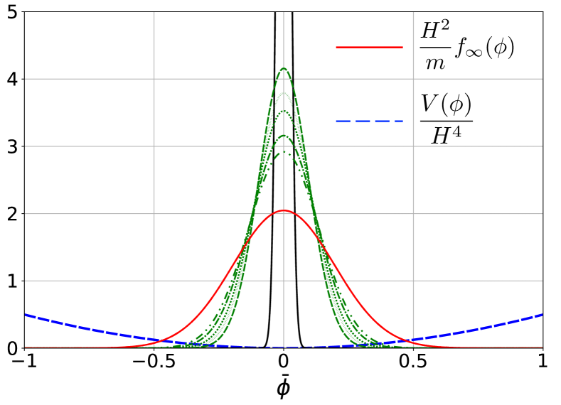
(a) PDF in time for $V(\phi)=m^{2}\phi^{2}/2$.

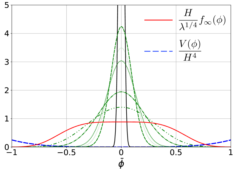
(b) PDF in time for $V(\phi)=\lambda\phi^{4}/4$.

Figure 1: Time evolution of the PDFs for $V(\phi)=m^{2}\phi^{2}/2$ (left) and $V(\phi)=\lambda\phi^{4}/4$ (right). The black, red, and green lines represent respectively the initial, stationary, and transient distributions. The blue lines correspond to the scalar potentials. The narrow Gaussian function, $f_{0}(\phi)=e^{-\phi^{2}/2\sigma^{2}}/\sqrt{2\pi}\,\sigma$, is used as the initial distribution where $\sigma=0.02$, in order to mimick the idealized $\delta$-function, Eq. (2.7). Here, the Crank–Nicolson scheme was used to numerically solve the Fokker–Planck equation (2.5).

Throughout this paper, we consider a scalar field in a quadratic or quartic potential,

$$V(\phi)=\begin{cases}\displaystyle\frac{m^{2}}{2}\phi^{2}&(\text{quadratic})\,\,,\\[8.61108pt] \displaystyle\,\,\frac{\lambda}{4}\,\,\phi^{4}&(\text{quartic})\,\,.\end{cases}$$ (2.11)

Figure 1 shows the time evolution of the PDFs obtained by a numerical resolution of the Fokker–Planck equation (2.5) for each potential. The stationary PDFs are obtained from Eq. (2.6),

$$f_{\infty}(\phi)=\begin{cases}\displaystyle\frac{m}{H^{2}}\sqrt{\frac{4\pi}{3}}\exp\quantity[-\frac{4\pi^{2}}{3}\quantity(\frac{m}{H^{2}}\phi)^{2}]&(\text{quadratic})\,\,,\\[8.61108pt] \displaystyle\frac{\lambda^{1/4}}{H}\frac{2}{\Gamma(1/4)}\quantity(\frac{2\pi^{2}}{3})^{1/4}\exp\quantity[-\frac{2\pi^{2}}{3}\quantity(\frac{\lambda^{1/4}}{H}\phi)^{4}]&(\text{quartic})\,\,.\end{cases}$$ (2.12)

For $V(\phi)=m^{2}\phi^{2}/2$, the system conserves at late times an exactly Gaussian behaviour (actually, the distribution can be shown analytically to be Gaussian at any time, and the time-dependent standard deviation can be computed exactly), while for $V(\phi)=\lambda\phi^{4}/4$ a negative kurtosis develops. The two-point function at equilibrium reads

$$\expectationvalue{\phi^{2}}_{\infty}\equiv\lim_{N\to\infty}\expectationvalue{\phi^{2}}(N)=\begin{cases}\displaystyle\frac{3}{8\pi^{2}}\quantity(\frac{H^{2}}{m})^{2}&(\text{quadratic})\,\,,\\[8.61108pt] \displaystyle\sqrt{\frac{3}{2\pi^{2}}}\frac{\Gamma(3/4)}{\Gamma(1/4)}\quantity(\frac{H}{\lambda^{1/4}})^{2}&(\text{quartic})\,\,,\end{cases}$$ (2.13)

and

$$\expectationvalue{\phi^{4}}_{\infty}=\begin{cases}\displaystyle\frac{27}{64\pi^{4}}\quantity(\frac{H^{2}}{m})^{4}&(\text{quadratic})\,\,,\\[8.61108pt] \displaystyle\frac{3}{8\pi^{2}}\quantity(\frac{H}{\lambda^{1/4}})^{4}&(\text{quartic})\,\,.\end{cases}$$ (2.14)

It is also possible to compute analytically the higher-order stationary correlation functions, e.g. in the quartic case one can compute the kurtosis, $\expectationvalue{\phi^{4}}_{\infty}/\expectationvalue{\phi^{2}}_{\infty}^{2}-3\approx-0.812$, showing that the $\lambda\phi^{4}$ theory is platykurtic in the equilibrium state PhysRevD.50.6357 .

For the time evolution of the correlation functions, recurrence relations for $a_{n,k}$ are obtained by substituting the expansion Eq. (2.9) into Eq. (2.10). For the two potentials, we find

$$(k+1)a_{n,k+1} =\displaystyle-\frac{m^{2}}{3H^{2}}na_{n,k}+\frac{H^{2}}{8\pi^{2}}n(n-1)a_{n-2,k} \text{(quadratic)}\,\,,$$ (2.15)

$$(k+1)a_{n,k+1} =\displaystyle-\frac{\lambda}{3H^{2}}na_{n+2,k}+\frac{H^{2}}{8\pi^{2}}n(n-1)a_{n-2,k} \text{(quartic)}\,\,.$$ (2.16)

In the following, we will focus for definiteness on the two-point function, the power spectrum (and the corresponding $a_{2,k}$). We will also apply the same tools, following the same steps, to the four-point function, the trispectrum (and the corresponding $a_{4,k}$). In principle, the time dependence of correlation functions of any order $n$ can be studied by these means.

$n\backslash k$	$0$	$1$	$2$	$3$	$4$	$5$	$6$	$\cdots$
$0$	$\pagecolor{blue!25}1$	$\pagecolor{blue!25}0$	$\pagecolor{blue!25}0$	$\pagecolor{blue!25}0$	$\pagecolor{blue!25}0$	$\pagecolor{blue!25}0$	$\pagecolor{blue!25}0$	$\pagecolor{blue!25}\cdots$
$1$	$\pagecolor{blue!25}0$	$\pagecolor{yellow!25}0$	$\pagecolor{yellow!25}0$	$\pagecolor{yellow!25}0$	$\pagecolor{yellow!25}0$	$\pagecolor{yellow!25}0$	$\pagecolor{yellow!25}0$	$\pagecolor{yellow!25}\cdots$
$2$	$\pagecolor{blue!25}0$	$\pagecolor{red!25}1/4\pi^{2}$	$-1/12\pi^{2}$	$1/54\pi^{2}$	$-1/324\pi^{2}$	$1/2430\pi^{2}$	$-1/21870\pi^{2}$	$\cdots$
$3$	$\pagecolor{blue!25}0$	$\pagecolor{yellow!25}0$	$\pagecolor{yellow!25}0$	$\pagecolor{yellow!25}0$	$\pagecolor{yellow!25}0$	$\pagecolor{yellow!25}0$	$\pagecolor{yellow!25}0$	$\pagecolor{yellow!25}\cdots$
$4$	$\pagecolor{blue!25}0$	$\pagecolor{yellow!25}0$	$\pagecolor{red!25}3/16\pi^{4}$	$-1/8\pi^{4}$	$7/144\pi^{4}$	$-1/72\pi^{4}$	$31/9720\pi^{4}$	$\cdots$
$5$	$\pagecolor{blue!25}0$	$\pagecolor{yellow!25}0$	$\pagecolor{yellow!25}0$	$\pagecolor{yellow!25}0$	$\pagecolor{yellow!25}0$	$\pagecolor{yellow!25}0$	$\pagecolor{yellow!25}0$	$\pagecolor{yellow!25}\cdots$
$6$	$\pagecolor{blue!25}0$	$\pagecolor{yellow!25}0$	$\pagecolor{yellow!25}0$	$\pagecolor{red!25}15/64\pi^{6}$	$-15/64\pi^{6}$	$25/192\pi^{6}$	$-5/96\pi^{6}$	$\cdots$
$\vdots$	$\pagecolor{blue!25}\vdots$	$\pagecolor{yellow!25}\vdots$	$\pagecolor{yellow!25}\vdots$	$\pagecolor{yellow!25}\vdots$	$\vdots$	$\vdots$	$\vdots$	$\ddots$

Table 1: The coefficients $\bar{a}_{n,k}$ for $V(\phi)=m^{2}\phi^{2}/2$. The colored entries are immediately determined from the initial and boundary conditions as well as the recurrence relations.

Quadratic case

For $V(\phi)=m^{2}\phi^{2}/2$, the recurrence relation can be solved analytically to give

$$\bar{a}_{2,k}=\begin{cases}\displaystyle 0&(k=0)\\[8.61108pt] \displaystyle-\frac{3}{8\pi^{2}}\frac{(-)^{k}}{k!}\quantity(\frac{2}{3})^{k}&(k\geq 1)\end{cases}\,\,,\qquad a_{n,k}=\bar{a}_{n,k}\frac{m^{2k}}{m^{n}}\frac{H^{2n}}{H^{2k}}\,\,,$$ (2.17)

where we introduced the rescaled coefficients $\bar{a}_{n,k}$ so that the recurrence relation reduces to $(k+1)\bar{a}_{n,k+1}=-(1/3)n\bar{a}_{n,k}+(1/8\pi^{2})n(n-1)\bar{a}_{n-2,k}$ for $n\geq 2$ and $k\geq 0$. From Eq. (2.17), the time dependence of the two-point function reads

$$\expectationvalue{\phi^{2}}(N)=\sum_{k=0}^{\infty}a_{2,k}N^{k}=\frac{3H^{4}}{8\pi^{2}m^{2}}\quantity[1-\exp\quantity(-\frac{2m^{2}}{3H^{2}}N)]\,\,,$$ (2.18)

and $\expectationvalue{\phi^{4}}=3\expectationvalue{\phi^{2}}^{2}$. The same expression can be obtained without expanding $\expectationvalue{\phi^{2}}$ in terms of $N$, by directly solving Eq. (2.10), the last term in the right hand side being a constant for $n=2$. Our conclusion regarding the expansion of $\expectationvalue{\phi^{2}}$ in terms of $N$, is that it results in a convergent series as it should be, therefore giving the exact formula Eq. (2.18). Any higher order correlation function can be computed this way for the quadratic case (another option is to compute them from the Gaussian density function $f(\phi,N)$), see Table 1 for a few other values of the $\bar{a}_{n,k}$.

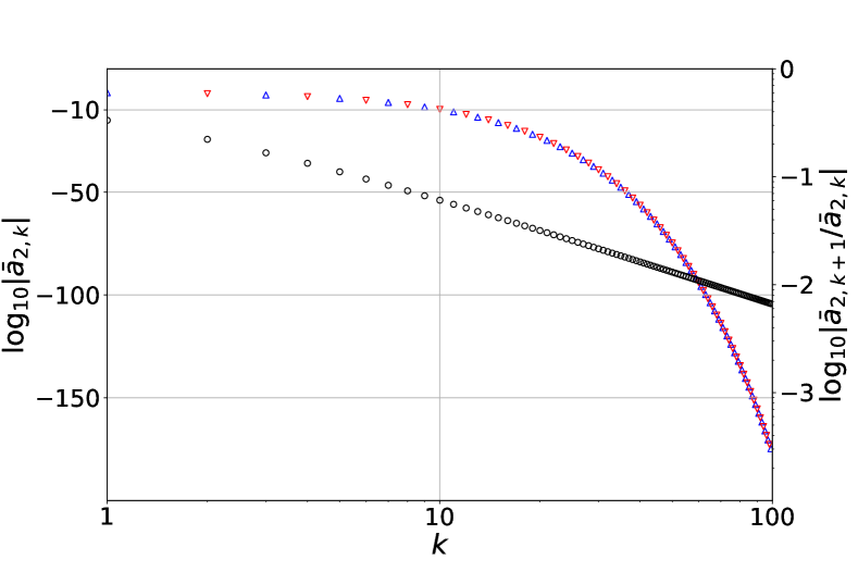
(a) Coefs. for $V(\phi)=m^{2}\phi^{2}/2$.

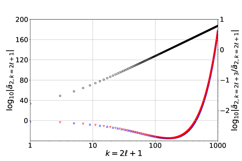
(b) Coefs. for $V(\phi)=\lambda\phi^{4}/4$.

Figure 2: The coefficients $\bar{a}_{2,k}$ and their ratio to the previous order, for the quadratic (left) and quartic (right) potentials. The upward and downward triangles indicate the sign of $\bar{a}_{2,k}$, and their absolute values can be read off from the left vertical axis. The circles are the ratio between neighboring two nonzero coefficients and can be read off from the right vertical axis.

The left panel of Fig. 2 shows the behaviour of the coefficients $\bar{a}_{2,k}$ and their ratio $\bar{a}_{2,k+1}/\bar{a}_{2,k}$ as $k$ increases. Noting that the ratio is related to the convergence radius $r_{c}$ of the series by

$$\frac{1}{r_{c}}=\lim_{k\to\infty}\absolutevalue{\frac{\bar{a}_{2,k+1}}{\bar{a}_{2,k}}}\,\,,$$ (2.19)

the plot implies that the expansion (2.18) indeed has an infinite convergence radius. The same holds for the equivalent expressions for $\expectationvalue{\phi^{4}}$. For convenience, we introduce dimensionless variables,

$$\expectationvalue{\bar{\phi}^{2}}=\sum_{k=0}^{\infty}\bar{a}_{2,k}\bar{N}^{k}\,\,;\qquad\bar{\phi}\equiv\frac{m}{H^{2}}\phi\,\,,\qquad\bar{N}\equiv\frac{m^{2}}{H^{2}}N\,\,,$$ (2.20)

then $a_{2,k}/a_{2,k+1}=(H^{2}/m^{2})\,\bar{a}_{2,k}/\bar{a}_{2,k+1}$. The top panels of Fig. 3 compares the series truncation of $\expectationvalue{\bar{\phi}^{2}}(\bar{N})$ and $\expectationvalue{\bar{\phi}^{4}}(\bar{N})$ at different orders with their exact results. We easily see that the series truncated at higher orders give better approximations over the whole region, as expected from the fact that the series (2.20) has an infinite radius of convergence.

$n\backslash k$	$0$	$1$	$2$	$3$	$4$	$5$	$6$	$\cdots$
$0$	$\pagecolor{blue!25}1$	$\pagecolor{blue!25}0$	$\pagecolor{blue!25}0$	$\pagecolor{blue!25}0$	$\pagecolor{blue!25}0$	$\pagecolor{blue!25}0$	$\pagecolor{blue!25}0$	$\pagecolor{blue!25}\cdots$
$1$	$\pagecolor{blue!25}0$	$\pagecolor{yellow!25}0$	$\pagecolor{yellow!25}0$	$\pagecolor{yellow!25}0$	$\pagecolor{yellow!25}0$	$\pagecolor{yellow!25}0$	$\pagecolor{yellow!25}0$	$\pagecolor{yellow!25}\cdots$
$2$	$\pagecolor{blue!25}0$	$\pagecolor{red!25}1/4\pi^{2}$	$0$	$-1/24\pi^{4}$	$0$	$1/80\pi^{6}$	$0$	$\cdots$
$3$	$\pagecolor{blue!25}0$	$\pagecolor{yellow!25}0$	$\pagecolor{yellow!25}0$	$\pagecolor{yellow!25}0$	$\pagecolor{yellow!25}0$	$\pagecolor{yellow!25}0$	$\pagecolor{yellow!25}0$	$\pagecolor{yellow!25}\cdots$
$4$	$\pagecolor{blue!25}0$	$\pagecolor{yellow!25}0$	$\pagecolor{red!25}3/16\pi^{4}$	$0$	$-3/32\pi^{6}$	$0$	$53/960\pi^{8}$	$\cdots$
$5$	$\pagecolor{blue!25}0$	$\pagecolor{yellow!25}0$	$\pagecolor{yellow!25}0$	$\pagecolor{yellow!25}0$	$\pagecolor{yellow!25}0$	$\pagecolor{yellow!25}0$	$\pagecolor{yellow!25}0$	$\pagecolor{yellow!25}\cdots$
$6$	$\pagecolor{blue!25}0$	$\pagecolor{yellow!25}0$	$\pagecolor{yellow!25}0$	$\pagecolor{red!25}15/64\pi^{6}$	$0$	$-15/64\pi^{8}$	$0$	$\cdots$
$\vdots$	$\pagecolor{blue!25}\vdots$	$\pagecolor{yellow!25}\vdots$	$\pagecolor{yellow!25}\vdots$	$\pagecolor{yellow!25}\vdots$	$\vdots$	$\vdots$	$\vdots$	$\ddots$

Table 2: The coefficients $\bar{a}_{n,k}$ for $V(\phi)=\lambda\phi^{4}/4$. The colored entries are immediately determined from the initial and boundary conditions as well as the recurrence relations.

Quartic case

For $V(\phi)=\lambda\phi^{4}/4$, the coefficients of $N^{k}$ can be rescaled as $a_{n,k}=\bar{a}_{n,k}H^{n}\lambda^{(2k-n)/4}$, and the recurrence relation reduces to $(k+1)\bar{a}_{n,k+1}=-(n/3)\bar{a}_{n+2,k}+(1/8\pi^{2})n(n-1)\bar{a}_{n-2,k}$. The closed form for general $\bar{a}_{2,k}$ is too complicated for practical use but again can be obtained. For even indices $k=0,\,2,\,\cdots$ the coefficient $\bar{a}_{2,k}$ vanishes, while for odd $k=1,\,3,\,\cdots$ it starts with $\bar{a}_{2,k=1}=1$ and

$$\bar{a}_{2,k}=\quantity(\frac{3}{2\pi^{2}})^{1/2}\frac{(-)^{(k-1)/2}}{k!}\quantity(\frac{1}{24\pi^{2}})^{k/2}\prod_{j=0}^{\frac{k-3}{2}}\sum_{p_{j}=j+2}^{p_{j+1}}(2p_{j}-2j-2)(2p_{j}-2j-1)(2p_{j}-2j)\,\,,$$ (2.21)

for $k=3,\,5\,\cdots$. In this expression, $p_{(k-1)/2}$ is given by $p_{(k-1)/2}=(k+1)/2$. This closed form is obtained for the first time to the best of the authors’ knowledge. Table 2 shows the first few terms of $\bar{a}_{n,k}$ for the quartic case. The coefficients for $n=2$ can be obtained from Eq. (2.21) or iteratively from Eq. (2.16), and the first terms are in precise agreement with the result from more detailed field theoretical calculations (see TSAMIS2005295 ; PhysRevD.79.044007 for the same recursive calculations and PhysRevD.76.043512 for field theoretical derivations). Although one may expect from Table 2 that the $e$-folding expansion of $\expectationvalue{\phi^{2}}$ is again convergent, it is not the case. In order to see this, we introduce dimensionless variables similar to Eq. (2.20),

$$\expectationvalue{\bar{\phi}^{2}}=\sum_{k=0}^{\infty}\bar{a}_{2,k}\bar{N}^{k}\,\,;\qquad\bar{\phi}\equiv\frac{\lambda^{1/4}}{H}\phi\,\,,\qquad\bar{N}\equiv\lambda^{1/2}N\,\,.$$ (2.23)

The right panel of Fig. 2 shows $\bar{a}_{2,k=2\ell+1}$ and $\bar{a}_{2,k=2\ell+3}/\bar{a}_{2,k=2\ell+1}$ for the case of the quartic potential. We see that the ratio exhibits a power-law growth with a positive exponent, which is typical of factorially divergent series that appear in various systems in physics. Therefore the plot implies that the convergent radius of the expansion Eq. (2.23) is zero in contrast to the quadratic case. Behaviour consistent with this can be seen in the bottom panels of Fig. 3, which compare truncated series with the numerical results. We see that higher order truncations start to blow up for smaller $\bar{N}$. This is typical behaviour of a series with a vanishing radius of convergence, and its naive summation to the infinite order does not make sense; we just get infinity everywhere except $\bar{N}=0$. This calls for some resummation prescription in order to recover the correct time evolution.

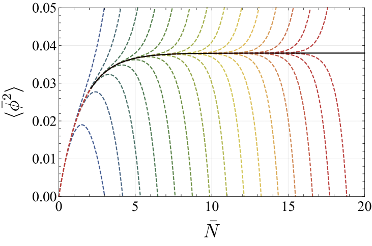
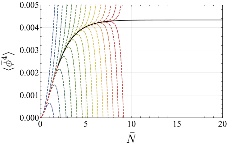
(a) Truncation for $V(\phi)=m^{2}\phi^{2}/2$.	(b) Truncation for $V(\phi)=m^{2}\phi^{2}/2$.
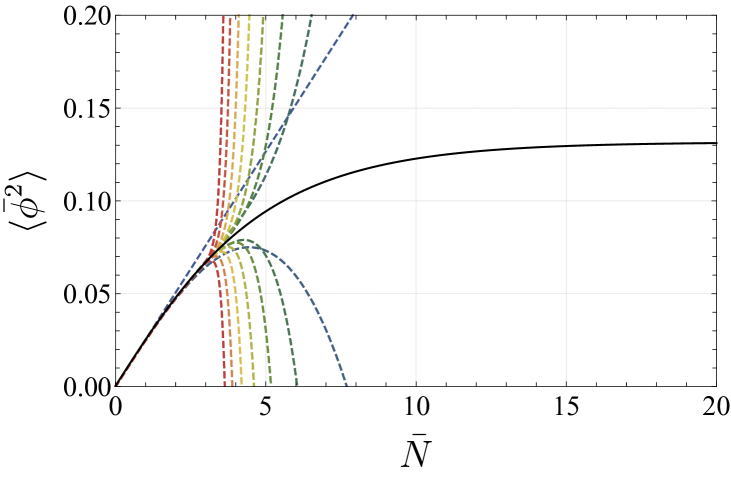
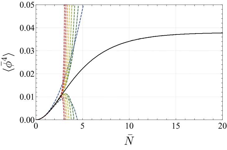
(c) Truncation for $V(\phi)=\lambda\phi^{4}/4$.	(d) Truncation for $V(\phi)=\lambda\phi^{4}/4$.

Figure 3: Series truncation of the correlations $\expectationvalue{\bar{\phi}^{2}}(\bar{N})$ (left) and $\expectationvalue{\bar{\phi}^{4}}(\bar{N})$ (right), for the quadratic (top) and quartic (bottom) potentials. The truncation orders $k_{\rm T}$ are set to be $k_{\rm T}=2,\,3,\,\dots,\,30$, and $k_{\rm T}$ increases from blue to red.

3 Time evolution of the correlation function from resummation

The closed form of $\bar{a}_{2,k}$ obtained in Eq. (2.21) for the quartic potential gives the information on all orders, and thus in principle gives the exact correlation function $\expectationvalue{\bar{\phi}^{n}}$. As mentioned in Sec. 2, however, it is practically difficult to obtain all the coefficients analytically, and so is the time evolution of the correlation function. To make matters worse, its $e$-folding expansion is a formal perturbative series that deviates more and more from its original behaviour as the order of truncation increases, as shown in the bottom panels of Fig. 3. In order to tame the divergence, we consider two kinds of resummation methods in this section, namely the Padé approximant and the Borel–Padé resummation.

3.1 Padé approximant: Approximating the exact behaviour by a rational function

The Padé approximant baker1996pade approximates a function by a rational function, in such a way that its power series agrees with that of the original function up to a given order. It often gives a better approximation of the original function than the naïvely truncated series, and it can be used even when the power series of the original function is divergent. We apply this procedure to the correlation functions of the spectator field.

The Padé approximant is constructed as follows. With a pair of integers $m,\,n\in\mathbb{Z}_{\geq 0}$, a smooth function $f(z)$ is approximated by a rational function called the Padé approximant,

$$f(z)=\sum_{k=0}^{\infty}a_{k}z^{k}\quad\longrightarrow\quad f^{[m|n]}_{\mathrm{P}}(z)\equiv\frac{\displaystyle\sum_{k=0}^{m}b_{k}z^{k}}{\displaystyle\sum_{k=0}^{n}c_{k}z_{k}}=\frac{b_{0}+b_{1}z+b_{2}z^{2}+\cdots+b_{m}z^{m}}{c_{0}+c_{1}z+c_{2}z^{2}+\cdots+c_{n}z^{n}}\,\,.$$ (3.1)

We require that $f(z)$ and $f_{\mathrm{P}}^{[m|n]}(z)$ be related by $f(z)=f_{\mathrm{P}}^{[m|n]}(z)+\mathcal{O}(z^{m+n+1})$. Thus we need the first $m+n+1$ coefficients of the Taylor expansion of $f(z)$ around $z=0$, and the coefficients $b_{k}$ and $c_{k}$ in Eq. (3.1) are uniquely determined by

$$\evaluated{\derivative[\ell]{f(z)}{z}}_{z=0}=\evaluated{\derivative[\ell]{f_{\mathrm{P}}^{[m|n]}(z)}{z}}_{z=0}\,\,,\qquad\ell=0,\,1,\,\dots,\,m+n\,\,.$$ (3.2)

The set of conditions (3.2) can be translated into

$$\sum_{k=0}^{\ell}a_{k}c_{\ell-k}-b_{\ell}=0\,\,,\qquad\ell=0,\,1,\,\dots,\,m+n\,\,.$$ (3.3)

It is clear that $f^{[m|n]}_{\mathrm{P}}(z)$ reduces to the $m$-th order of the Taylor expansion of $f(z)$ when $n=0$. The special case, $m=n$, is called the diagonal Padé approximant, and it is known to often give a better approximation than the ones with $m\neq n$ called non-diagonal Padé approximants. In the following, however, we restrict ourselves to the non-diagonal choice with $m=p-1$ and $n=p+1$ for a positive integer $p$. This choice is made for the purpose of using the same order for the Padé approximants consistently throughout the paper: since the order of the Padé approximants used in Borel–Padé resummation, as we see in Sec. 3.2, is required to satisfy $m<n$ from the viewpoint of convergence, we use the same choice here. For completeness, in Appendix A we also show the result of diagonal Padé for $\expectationvalue{\phi^{2}}$ and $\expectationvalue{\phi^{4}}$.

Padé approximants have several important properties essentially coming from the fact that they are rational functions. First, Padé approximants cannot have branch cuts while they can have poles. This implies that when we try to approximate a function with branch cuts, Padé approximants cannot reproduce exactly the same analytic structure as the original function has. Instead, higher-order Padé approximants typically develop a bunch of poles and/or zeros around the location of the branch cut of the original function. For this reason, Padé approximants typically give better approximations for meromorphic functions than for functions with branch cuts. Second, the series expansion of a Padé approximant with a finite order around the origin is always convergent. This means that, when the original function has a divergent series around the origin, Padé approximants with a finite order cannot share this property. Thus, if we know some of the properties of the original function a priori, it is better to adopt an approximation scheme that correctly captures these properties. If otherwise, Padé approximants are usually a good first step to probe some of the properties.

From the above considerations, we construct the Padé approximants of the correlation functions as

$$\expectationvalue{\phi^{2}}(N)=\sum_{k=0}^{\infty}a_{2,k}N^{k}\quad\longrightarrow\quad\expectationvalue{\phi^{2}}_{\mathrm{P}}^{[p-1|p+1]}(N)=\frac{\displaystyle\sum_{k=0}^{p-1}b_{k}N^{k}}{\displaystyle\sum_{k=0}^{p+1}c_{k}N^{k}}\,\,,$$ (3.4)

and similarly for $\expectationvalue{\phi^{4}}$. Figure 4 shows the Padé approximant for both the quadratic and quartic potentials. Compared to Fig. 3, those indeed give improved behaviour compared to the naïvely truncated cases. Not only does the Padé approximant reproduce the transient regime around $\bar{N}\sim 10$, but it also gives the correct stationary behaviour, especially for the quadratic case. However, quantitatively, we see a difference in accuracy between the quadratic and quartic cases. In the quartic case, the approximation is relatively worse despite it uses higher order information, though it is still much better than the truncated series. In the quadratic case, the exact results are entire functions and the Padé approximant is good at approximating such functions. As mentioned above, the quartic case has a divergent perturbative series and its Padé approximant with a finite order cannot have such a property. Therefore the Padé approximant is likely worse at approximating functions having divergent series compared to analytic functions. This motivates us to consider another resummation scheme that efficiently takes the properties of the series into account.

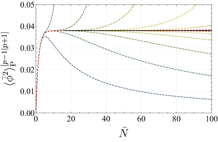
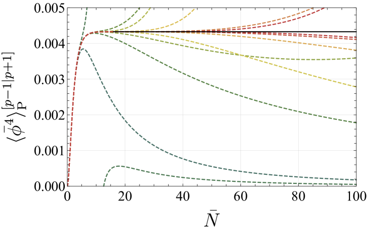
(a) Direct Padé for $V(\phi)=m^{2}\phi^{2}/2$.	(b) Direct Padé for $V(\phi)=m^{2}\phi^{2}/2$.
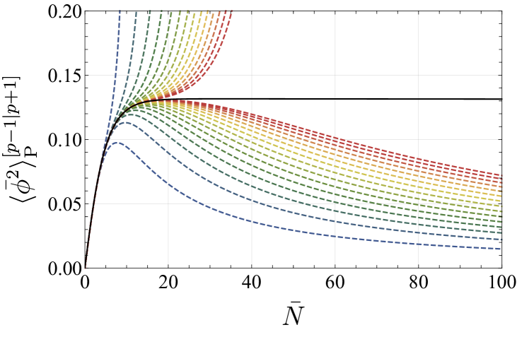
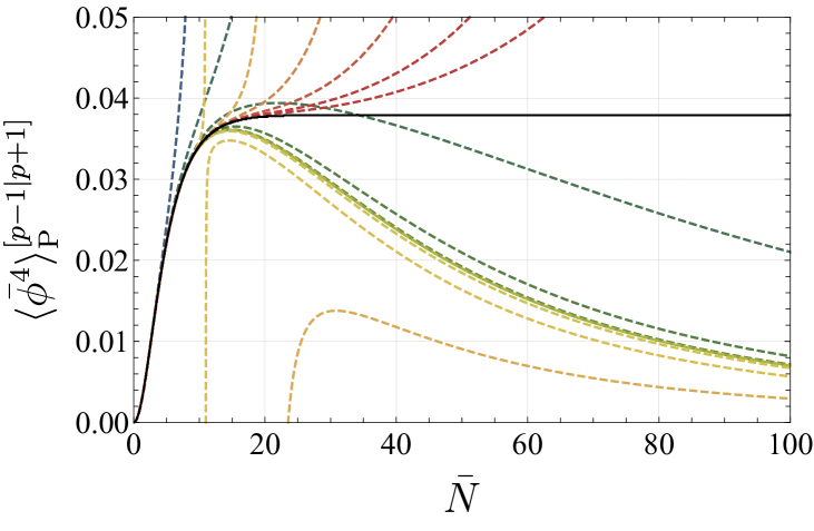
(c) Direct Padé for $V(\phi)=\lambda\phi^{4}/4$.	(d) Direct Padé for $V(\phi)=\lambda\phi^{4}/4$.

Figure 4: Direct Padé approximants $\expectationvalue{\bar{\phi}^{2}}_{\textrm{P}}^{[p-1|p+1]}(\bar{N})$ (left) and $\expectationvalue{\bar{\phi}^{4}}_{\textrm{P}}^{[p-1|p+1]}(\bar{N})$ (right), for the quadratic (top, up to $p=15$) and quartic (bottom, up to $p=30$) potentials. The order $p$ increases from blue to red.

One may wonder what if we use diagonal Padé, since in the diagonal case the highest orders of the numerator and denominator in Eq. (3.1) are the same, and thus the asymptotic stationary behavior of the correlation functions is guaranteed. Interestingly, however, this improvement applies only to some of the correlation functions (more specifically, $\expectationvalue{\phi^{4}}$, $\expectationvalue{\phi^{8}}$, $\cdots$). We illustrate this point in Appendix A.

3.2 Borel resummation: Extracting the correct information from a formal series

In the last subsection we saw how the Padé approximant reproduces the original correlation functions up to some moderate $e$-folding number, even when the original power series is divergent and defined only formally. However, we also found that in the quartic case the approximation is relatively worse presumably because this case has a divergent perturbative series and the Padé approximant is likely worse at approximating such functions than analytic functions. Here we take another strategy: Borel–Padé resummation. It is a combination of Borel resummation and Padé approximation, and there are also other motivations beyond the above to use it in the present context. Here, we take another strategy: Borel resummation (or practically Borel–Padé resummation, use of Padé approximation in Borel summation.) There are also other motivations beyond the above to use it in the present context. First, correlation functions in de Sitter spacetime are expected to reach asymptotic values for sufficiently large $N$. As we see below, the Borel transformation of such functions in general converges to zero in the Borel plane. This property makes it easier to approximate the function with the Padé approximation, and thus we expect that the behaviour of the divergent series is improved even more with Borel–Padé resummation. Second, Borel transformation contains information about possible non-perturbative aspects of the system through the singularity structure in the Borel plane, and thus is physically interesting to investigate. In the following we illustrate how this method works for the correlation functions in de Sitter space.

Borel resummation ASENS_1899_3_16__9_0 ; bender78:AMM ; SPT:KT is defined through the Borel transformation of the original series. For an infinite series with respect to $z$ and $\alpha\notin\mathbb{Z}_{\leq 0}$,

$$f(z)=\sum_{k=0}^{\infty}a_{k}z^{k+\alpha}\,\,,$$ (3.5)

we define the Borel transformation of $f(z)$ by

$$f_{\mathrm{B}}(t)\equiv\sum_{k=0}^{\infty}\frac{a_{k}}{\Gamma(k+\alpha)}t^{k+\alpha-1}\,\,.$$ (3.6)

Then the Borel resummation of $f(z)$ is defined as

$$f_{\mathrm{S}}(z)\equiv\int_{0}^{\infty}\differential t\,e^{-t/z}\widetilde{f_{\mathrm{B}}}(t)\,\,,$$ (3.7)

where $\widetilde{f_{\rm B}}(t)$ is a simple analytic continuation of the series (3.6). The Borel resummation (3.7) has the following important properties. First, it has the same asymptotic behavior around $z=0$ as the original one (3.5) (up to exponentially suppressed corrections that may appear). One can easily check this by expanding $\widetilde{f_{\rm B}}(t)$ around $t=0$ as in Eq. (3.6) and then exchanging the order of the $t$-integration and the expansion. Second, the Borel resummation can be finite for finite and non-zero $z$ under some conditions (explained later), even if the original perturbative series (3.5) is divergent. Because of these reasons, the Borel resummation may correctly capture the true properties of the original function and has turned out to be the most standard way to resum divergent perturbative series.

Let us emphasize the contexts in which Borel resummation works. The Borel resummation, Eq. (3.7), reproduces the original function $f(z)$ when $f(z)$ is analytic as demonstrated below in the quadratic case. In this case, $f(z)$ is the same as a simple analytic continuation of the perturbative series summed inside its convergence radius, and correspondingly the Borel transformation, Eq. (3.6), has an infinite radius of convergence allowing us to exchange the order of the integral and series expansion in Eq. (3.7). On the other hand, if $f(z)$ gives a divergent series but its Borel resummation is convergent, then $f_{\mathrm{S}}(z)$ is a function that has the same asymptotic behaviour as $f(z)$ and is convergent (in some angular domain in $z$-plane). In this sense, the Borel resummation endows the original formal series with an analytical meaning. However, one or more singular points may appear along the contour of the integral (i.e. the real $t$ axis), and in such cases uncertainties arise as to how to avoid them. These ambiguities are typically related to non-perturbative aspects of the physical system. However, we will see below that the correlation functions considered in the present paper have no such singularities and thus are free from uncertainties, allowing for unambiguous resummation.

Before applying Borel resummation to the divergent series of the quartic potential, let us demonstrate how it works for an exactly solvable case, the stochastic spectator in the quadratic potential. One starts with the original series (2.18),

$$\expectationvalue{\bar{\phi}^{2}}(\bar{N})=\sum_{k=0}^{\infty}\bar{a}_{2,k}\bar{N}^{k}=\sum_{k=1}^{\infty}\bar{a}_{2,k}\bar{N}^{k}=\sum_{k=0}^{\infty}\bar{a}_{2,k+1}\bar{N}^{k+1}\,\,,$$ (3.8)

where we used $\bar{a}_{2,0}=0$, then the Borel transformation of Eq. (2.18) is obtained as

$$\expectationvalue{\bar{\phi}^{2}}_{\mathrm{B}}(t)=\sum_{k=0}^{\infty}\frac{a_{2,k+1}}{\Gamma(k+1)}t^{k}=\evaluated{\frac{1}{2\pi^{2}}\frac{I_{1}(2s)}{2s}}_{s^{2}=-2t/3}\,\,,$$ (3.9)

where $I_{\nu}(z)$ is the modified Bessel function of the first kind, and we used

$$I_{\nu}(z)=\sum_{k=0}^{\infty}\frac{1}{k!\Gamma(\nu+k+1)}\quantity(\frac{z}{2})^{\nu+2k}\,\,.$$ (3.10)

Note that $t$ appearing in Eq. (3.9) is just an auxiliary variable and has nothing to do with the time variable. The absence of singularity in the Borel transformation (3.9) in $t\in[0,\,\infty)$ implies that the system is free from non-perturbative effects and that the succeeding Laplace integral can be performed without any ambiguity. One sees that the Borel transformation (3.9) vanishes as $t\to\infty$, and this behaviour guarantees the relaxation of the correlators of the stochastic field that obeys the Langevin equation. From Eq. (3.9) we obtain the Borel resummation of $\expectationvalue{\phi^{2}}$ as

$$\expectationvalue{\bar{\phi}^{2}}_{\mathrm{S}}(\bar{N})=\int_{0}^{\infty}\differential t\,e^{-t/\bar{N}}\expectationvalue{\bar{\phi}^{2}}_{\mathrm{B}}(t)=\frac{3}{8\pi^{2}}\quantity[1-\exp\quantity(-\frac{2}{3}\bar{N})]\,\,.$$ (3.11)

Here we used the identity Gradshteyn:1702455 ,

$$\int_{0}^{\infty}\differential z\,e^{-\alpha z^{2}}I_{\nu}(\beta z)=\frac{1}{2}\sqrt{\frac{\pi}{\alpha}}\exp\quantity(\frac{\beta^{2}}{8\alpha})I_{\nu/2}\quantity(\frac{\beta^{2}}{8\alpha})\,\,,\quad\real\nu>-1\,\,,\quad\real\alpha>0\,\,.$$ (3.12)

As we see from this example, when the original function is an entire function (more generally analytic function), the Borel transformation is free from singularities everywhere and we can safely perform the Laplace integral to reproduce the original function exactly.

3.3 Borel–Padé resummation for a stochastic spectator in the quartic potential

Let us apply Borel resummation to the spectator in the quartic potential. Since the expansion coefficients $\bar{a}_{2,k}$ for even $k$’s vanish, we may remove these coefficients,

$$\expectationvalue{\bar{\phi}^{2}}(\bar{N})=\sum_{k=0}^{\infty}\bar{a}_{2,k}\bar{N}^{k}=\sum_{\ell=0}^{\infty}\bar{a}_{2,2\ell+1}\bar{N}^{2\ell+1}\,\,.$$ (3.13)

In order to apply Eq. (3.5) with $\bar{N}^{2}$ being the expansion parameter, we regard Eq. (3.13) as

$$\bar{N}\expectationvalue{\bar{\phi}^{2}}(\bar{N})=\sum_{\ell=0}^{\infty}\bar{a}_{2,2\ell+1}(\bar{N}^{2})^{\ell+1}\,\,.$$ (3.14)

Borel transformation is applied to Eq. (3.14),

$$\quantity[\bar{N}\expectationvalue{\bar{\phi}^{2}}]_{\mathrm{B}(\bar{N}^{2})}(t)=\sum_{k=0}^{\infty}\frac{\bar{a}_{2,2k+1}}{k!}t^{k}\,\,.$$ (3.15)

Note that the subscript $\mathrm{B}(\bar{N}^{2})$ indicates that we perform Borel transformation with $\bar{N}^{2}$ being the expansion parameter. The Laplace integral of Eq. (3.15) gives the Borel summation of $\bar{N}\expectationvalue{\bar{\phi}^{2}}$. Then, the Borel summed correlator reads

$$\expectationvalue{\bar{\phi}^{2}}_{\mathrm{S}(\bar{N}^{2})}(\bar{N})=\frac{1}{\bar{N}}\int_{0}^{\infty}\differential t\,e^{-t/\bar{N}^{2}}\quantity[\bar{N}\expectationvalue{\bar{\phi}^{2}}]_{\mathrm{B}(\bar{N}^{2})}(t)\,\,.$$ (3.16)

The above procedure gives the Borel resummation for the formal series (2.23) if all the coefficients $\bar{a}_{2,k}$ are available. However, in the present case, it is practically impossible to have all of them as we saw in Sec. 2. In this situation, one of the standard prescription is to approximate the Borel transformation with a Padé approximant and then perform Laplace transformation. This method is called Borel–Padé resummation. First, the original series is truncated at a finite order, and from it the (truncated) Borel transformation is constructed. The Padé approximant is used here giving the Borel–Padé transformation of $\bar{N}\expectationvalue{\bar{\phi}^{2}}(\bar{N})$,

$$\quantity[\bar{N}\expectationvalue{\bar{\phi}^{2}}]_{\mathrm{BP}(\bar{N}^{2})}^{[p-1|p+1]}(t)=\quantity[\sum_{k=0}^{\infty}\frac{\bar{a}_{2,2k+1}}{k!}t^{k}]_{\mathrm{P}}^{[p-1|p+1]}\,\,,$$ (3.17)

and we finally obtain the Borel–Padé resummation,

$$\expectationvalue{\bar{\phi}^{2}}_{\mathrm{SP}(\bar{N}^{2})}^{[p-1|p+1]}(\bar{N})=\frac{1}{\bar{N}}\int_{0}^{\infty}\differential t\,e^{-t/\bar{N}^{2}}\quantity[\bar{N}\expectationvalue{\bar{\phi}^{2}}]_{\mathrm{BP}(\bar{N}^{2})}^{[p-1|p+1]}(t)\,\,.$$ (3.18)

In general, a Padé approximant has one or more poles since it is a rational function by definition. Some of them are apparent ones that can (dis)appear depending on the choice of the order $p$, while others are manifestation of the singularities that the exact Borel transformation has. As we will see in Sec. 3.4, the Borel–Padé transformations have no poles on the positive real axis (except for some apparent ones, see for example the blue curves in Fig. 5). Hence, whenever the Borel–Padé transformations $\quantity[\bar{N}\expectationvalue{\bar{\phi}^{2}}]_{\mathrm{BP}(\bar{N}^{2})}^{[p-1|p+1]}(t)$ and $\expectationvalue{\bar{\phi}^{4}}_{\mathrm{BP}(\bar{N}^{2})}^{[p-1|p+1]}(t)$ at some order $p$ have those apparent poles on the integration contour, we evaluate the Laplace integral (3.18) taking the principal values at these poles.

Figure 5 shows the Borel–Padé transformation at different orders $p$ in the Laplace space (i.e. as a function of $t$). The left and right panels are $\quantity[\bar{N}\expectationvalue{\bar{\phi}^{2}}]_{\mathrm{BP}(\bar{N}^{2})}^{[p-1|p+1]}(t)$ and $\expectationvalue{\bar{\phi}^{4}}_{\mathrm{BP}(\bar{N}^{2})}^{[p-1|p+1]}(t)$, respectively. Figure 6 shows the result of the Borel–Padé resummation, with the left and right panel being $\expectationvalue{\bar{\phi}^{2}}_{\mathrm{SP}(\bar{N}^{2})}^{[p-1|p+1]}(\bar{N})$ and $\expectationvalue{\bar{\phi}^{4}}_{\mathrm{SP}(\bar{N}^{2})}^{[p-1|p+1]}(\bar{N})$, respectively. For comparison, we also show the result of the direct Padé in grey. We see that both the transient and stationary behaviour are nicely reproduced, and that the Borel–Padé improves the approximation compared to the direct Padé in Fig. 4. This is the main result of this paper.

Note that Eq. (3.14) regards $\bar{N}^{2}$ as the expansion parameter rather than $\bar{N}$. When the initial condition for the spectator field is taken arbitrary, one cannot necessarily regard the former to be the expansion parameter since the coefficients $\bar{a}_{n,k}$ may have non-zero entries for both odd and even orders of $k$. We show in Appendix A that Borel–Padé transformation works even in such cases.

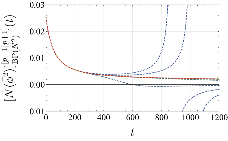
(a) Borel–Padé transf. for $V(\phi)=\lambda\phi^{4}/4$.

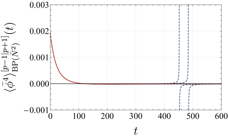
(b) Borel–Padé transf. for $V(\phi)=\lambda\phi^{4}/4$.

Figure 5: Borel–Padé transformation $\quantity[\bar{N}\expectationvalue{\bar{\phi}^{2}}]_{\mathrm{BP}(\bar{N}^{2})}^{[p-1|p+1]}(t)$ (left) and $\expectationvalue{\bar{\phi}^{4}}_{\mathrm{BP}(\bar{N}^{2})}^{[p-1|p+1]}(t)$ (right) for $V=\lambda\phi^{4}/4$. The orders are $p=2,\,3,\,\dots,\,30$, and $p$ increases from blue to red. Some of the curves are degenerate.

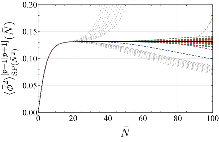
(a) Borel–Padé resummation for $V(\phi)=\lambda\phi^{4}/4$.

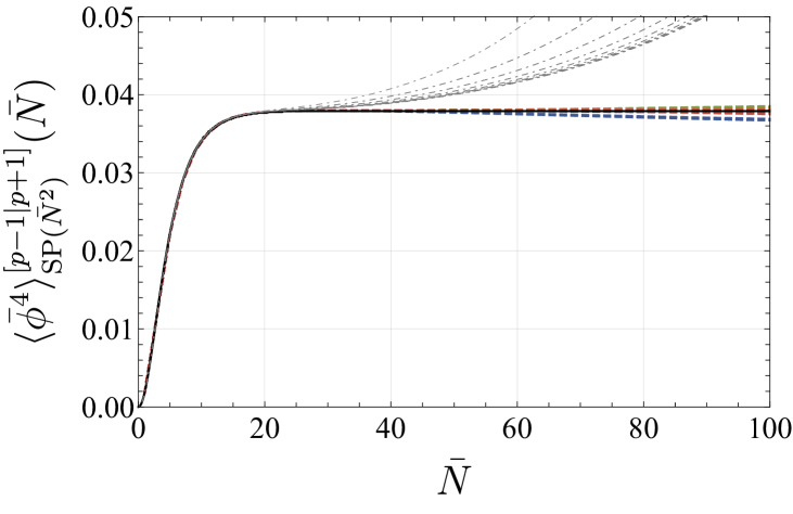
(b) Borel–Padé resummation for $V(\phi)=\lambda\phi^{4}/4$.

Figure 6: The Borel–Padé resummation $\expectationvalue{\bar{\phi}^{2}}_{\mathrm{SP}(\bar{N}^{2})}^{[p-1|p+1]}(\bar{N})$ (left) and $\expectationvalue{\bar{\phi}^{4}}_{\mathrm{SP}(\bar{N}^{2})}^{[p-1|p+1]}(\bar{N})$ (right) for $V=\lambda\phi^{4}/4$. The orders are $p=16,\,\dots,\,50$, and $p$ increases from blue to red, while the black solid lines correspond to the numerically calculated behaviour. In the right panel, most of all the curves are degenerate. The direct Padé approximants for $p=30,\,\dots,\,50$ are also plotted with grey dotted-dashed curves for comparison.

3.4 Singularity structure in the Borel plane

In this subsection we finally study the singularity structure in the Borel plane for $V(\phi)=\lambda\phi^{4}/4$. The singularity structure is important for the following reasons. First, the location of the singularities affects whether the Borel resummation is well-defined: the integral contour of the Laplace transformation may hit the singularities and hence we should check if it happens. Second, it is known that singularities of the Borel transformation are typically related to non-perturbative effects and Stokes phenomena. While we do not have an exact expression for the Borel transformation in the current problem, it is natural to expect that the Borel–Padé transformation reflects the original singularity structure to some extent. Thus in the following we estimate it through the Borel–Padé transformation.

Figure 7 shows how the poles (red crosses) and zeros (blue circles) in the Borel–Padé transformation of $\bar{N}\expectationvalue{\bar{\phi}^{2}}(\bar{N})$ and $\expectationvalue{\bar{\phi}^{4}}(\bar{N})$ change as the order $p$ increases. We observe several clusters in which poles and zeros appear alternately: one is located along the negative real axis, and the others form curves in the left half of the $t$-plane. In all the three curves the poles and zeros appear alternately, and the three curves are relatively stable against the change in the order of the Padé approximant. These facts suggest that these poles and zeros inherit the branch cuts that the exact Borel transformation has yamada2014numerical . One of the cuts lies along the negative real axis, and it starts from $t=t_{0}\simeq-80$. The starting point $t=t_{0}$ determines the convergence radius of the series expansion of the exact Borel transformation. The others extend to the real negative axis as the order $p$ increases. The existence of the cuts signals that there are Stokes phenomena when we extend $\bar{N}^{2}$ to complex region. However, practically this is not of much importance: what is important here is that we do not have cuts extended to the real and positive axis nor isolated poles on it, and thus the succeeding Laplace integral has no ambiguity arising from the way to circumvent the branch cuts or poles on the integration contour. This also suggests the absence of non-perturbative effects in the present system.

Other structures include isolated zeros that appear in all the panels in Fig. 7. However, zeros do not mean any singularities and thus they do not have much importance in the current analysis. Also, in identifying the location of the poles and zeros, care must be taken with numerical precision since the coefficients of the perturbative series are calculated with a finite numerical precision. Insufficient precision can lead to the emergence of ghost pairs in a characteristic way yamada2014numerical , and we explain this phenomenon in Appendix B.

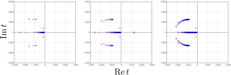
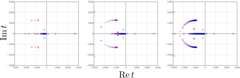
Figure 7: Distribution of the poles and zeros in the Borel–Padé transformation, $\quantity[\bar{N}\expectationvalue{\bar{\phi}^{2}}]_{\mathrm{BP}(\bar{N}^{2})}^{[p-1|p+1]}(t)$ (top) and $\expectationvalue{\bar{\phi}^{4}}_{\mathrm{BP}(\bar{N}^{2})}^{[p-1|p+1]}(t)$ (bottom), for $V=\lambda\phi^{4}/4$. Plots are made for $p=50$ (left), $p=150$ (middle), and $p=500$ (right). The appearance of alternating poles (red crosses) and zeros (blue circles) along the curves imply the existence of branch cuts in the exact Borel transformation.

4 Discussion and conclusions

In this paper, we discussed the application of the Padé approximation and Borel–Padé resummation in the context of the stochastic formalism of inflation, focusing on the dynamics of a spectator field. In the stochastic formalism, coarse-grained fields follow the Langevin equation and their distributions correspondingly follow the Fokker-Planck equation. In de Sitter spacetime, it is intuitively easy to understand that this is a system leading to an equilibrium state. In fact, the equilibrium distribution (2.6) and (2.8) can be easily calculated for an arbitrary potential, and the relaxation process is not difficult to obtain numerically (see Fig. 1). However, it is hard to grasp an analytical understanding of the out-of-equilibrium transition. One way is to perturbatively expand the correlation functions in terms of the $e$-folding number $N$. But the series are dangerously diverging for a wide class of potentials and can only be interpreted as formal series. They are therefore reputed to be trustworthy at early times only.

To investigate the properties of the correlation functions in stochastic inflation and the usefulness of the Padé approximation or the Borel–Padé resummation, we focused on the dynamics of spectator field in the paradigmatic $\lambda\phi^{4}$ setup in de Sitter spacetime. First, we confirmed that the expansion coefficients of the correlation functions increase more or less factorially with an alternating sign, suggesting that the radius of convergence of the series is zero (see the right panel of Fig. 2 and the bottom panels of Fig. 3). This is in contrast to the case of a quadratic drift, in which the system is analytically solvable and the coefficients monotonically decrease (see the left panel of Fig. 2). The Padé approximants may be useful in taming such diverging behaviour, and we first explored this possibility. They approximate a function by a rational function in such a way that the coefficients are determined so that the power series of the latter successively matches that of the former, and in many cases they reproduce the original function better than the naively truncated series. While the naively truncated series gets worse as the truncation order increases, the Padé approximants indeed reproduce the original functions better as the order increases, up to a certain $e$-folding, and not only around the transient regime but also until the equilibrium is reached (see Fig. 4).

While the Padé approximants are useful, we saw that they perform relatively worse in the quartic case presumably because this case has a divergent perturbative series and the Padé approximant is likely worse at approximating such functions than analytic functions as appeared in the quadratic case. This motivates us to apply the Borel–Padé resummation, where the Borel transformation is approximated by the Padé approximant. There are two other reasons to use this method. One is that the present system is an equilibrating one in which the correlation functions are expected to reach constant values, and in such a case, the Borel transformation converges to zero in the Borel plane as its argument $t$ goes to infinity. Due to this property, we expect good accuracy of the Padé approximant in Borel plane and the resulting Borel–Padé resummation. In fact, we confirmed that Borel–Padé resummation reproduces very well the behavior of the original correlation functions from the transient regime to the equilibrium regime (see Fig. 6). Another reason is the general expectation that the singularity structure in Borel plane tells us about non-perturbative properties of the original system. Although the singularity structure of the Borel transformation is not strictly known until all the expansion coefficients are available, its Padé approximation often inherits the original singularity structure. We found several clusters of the poles and zeros in the Borel–Padé transformations: one is along the real negative axis, and it stems from the convergence boundary. It has poles and zeros appearing in an alternate way, hence implying the existence of a branch cut. The others are located on curves, and again have poles and zeros appearing alternately, thus signalling other branch cuts. However, as these singularities do not appear on the positive real axis, we do not expect any non-perturbative effects present in the current setup. Therefore, the Laplace integral, the final step of the Borel(–Padé) resummation, can be performed without ambiguity.

We conclude by mentioning several possible applications of the analysis presented in this paper. First, it would be straightforward to extend the currents results to higher order $n$-point correlation functions within the same setup. A natural direction would then be to investigate to which extent one may reconstruct the full PDF in the relaxation process, from the time-dependent correlation functions. Second, in our analysis, the spectator field was assumed to start from the global minimum of $\mathbb{Z}_{2}$-symmetric potentials, which greatly simplified the recurrence structure. It would be interesting to study more general initial conditions, in which case those simplifications could not occur. Third, another possibility would be to study more nontrivial potentials such as the double well potential leading to phase transitions in the early universe, and to investigate the relation between the singularity structure and non-perturbative effects. Indeed, the one-loop correction to the instanton contribution to the correlation function can be seen in the stochastic framework.

Last but not least, the case of the stochastic field being the inflaton field and therefore leading the expansion of the universe, would be of great importance. For this purpose one should take the field dependence of the Hubble parameter into account, as given by the Friedmann equation in the slow-roll approximation, $3H^{2}M_{\mathrm{Pl}}^{2}\simeq V(\phi)$. One can already anticipate several other complications, such as the fact that the discretisation of the time scheme of the Langevin equations could affect the final result. Then, since fluctuations of the inflaton can be converted to those of the curvature perturbation through the stochastic $\delta N$ formalism, one can treat the latter within the stochastic framework in a non-perturbative way. One of the interesting consequences of this approach is that the PDF of the curvature perturbation typically develops an exponential tail, which can be expected to lead to a more efficient PBH formation scenario than the same setup investigated with the conventional linear perturbation theory. Understanding the exponential tail from the viewpoint of singularities in the Borel space is definitely a thrilling future direction. We leave such considerations for future work.

Appendix A Different choices for Padé approximant and Borel–Padé summation

Direct Padé

In the main text we used the non-diagonal Padé $[p-1|p+1]$ for the direct Padé approximation. However, since one knows that the correlators approach constant values for $N\to\infty$, one may wonder if diagonal Padé performs better. Actually this is true for $\expectationvalue{\phi^{4}},\expectationvalue{\phi^{8}},\cdots$ while not for $\expectationvalue{\phi^{2}},\expectationvalue{\phi^{6}},\cdots$. In Fig. 8 we show the results for the direct diagonal Padé. The left panel is for $\expectationvalue{\phi^{2}}_{\textrm{P}}^{[p|p]}$ while the right panel is for $\expectationvalue{\phi^{4}}_{\textrm{P}}^{[p|p]}$. The former does not show significant improvement compared to the left panel of Fig. 4, while the latter improves drastically from the right panel of Fig. 4.

The reason for the behavior of the correlators $\expectationvalue{\phi^{2}},\expectationvalue{\phi^{6}},\cdots$ can be explained in the following way. Consider $\tanh x$, which approaches a constant for $x\to\infty$ and has only odd powers of the argument when expanded around zero:

$$\tanh x =x-\frac{1}{3}x^{3}+\frac{2}{15}x^{5}-\frac{17}{315}x^{7}+\cdots.$$ (A.1)

Applying diagonal Padé approximation, one obtains

$$[\tanh x]_{\mathrm{P}}^{[1|1]} =x\,\,,\quad[\tanh x]_{\mathrm{P}}^{[2|2]}=\frac{x}{\displaystyle 1+\frac{x^{2}}{3}}\,\,,\quad[\tanh x]_{\mathrm{P}}^{[3|3]}=\frac{\displaystyle x+\frac{x^{3}}{15}}{\displaystyle 1+\frac{2x^{2}}{5}}\,\,,\quad\cdots\,\,.$$ (A.2)

As clear from these expressions, diagonal Padé does not necessary mean that the highest order terms for the numerator and/or denominator are nonzero. According to table 2, this class of correlators has only terms with odd powers of $N$ and thus cannot improved by the diagonal choice for the Padé approximants.

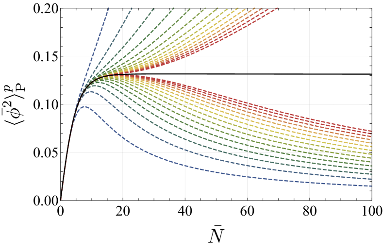
(a) $V(\phi)=\lambda\phi^{4}/4$.

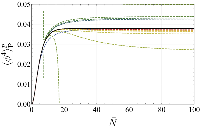
(b) $V(\phi)=\lambda\phi^{4}/4$.

Figure 8: Direct diagonal Padé approximation $\expectationvalue{\bar{\phi}^{2}}_{\textrm{P}}^{[p|p]}(\bar{N})$ (left) and $\expectationvalue{\bar{\phi}^{4}}_{\textrm{P}}^{[p|p]}(\bar{N})$ (right) for $V=\lambda\phi^{4}/4$. The orders are $p=2,\,\cdots,\,30$ and $p$ increases from blue to red.

Borel–Padé resummation

In Sec. 3, we applied Borel transformation with $\bar{N}^{2}$ being the fundamental expansion parameter, see Eq. (3.14). However, we may not always do this since the coefficients $a_{n,k}$ may have full entries depending on the initial condition for the spectator field. In this appendix, therefore, we show how the results change for Borel–Padé resummation with $\bar{N}$ being the expansion parameter.

We first show in Fig. 9 the Borel–Padé transformation with $\bar{N}$ being the expansion parameter, using the same orders for the approximants as Sec. 3.3. This corresponds to using the full coefficients $\bar{a}_{2,k+1}$, not $\bar{a}_{2,2k+1}$, and $[m|n]=[p-1|p+1]$,

$$\expectationvalue{\bar{\phi}^{2}}_{\mathrm{BP}(\bar{N})}^{[p-1|p+1]}(t) =\quantity[\sum_{k=0}^{\infty}\frac{\bar{a}_{2,k+1}}{k!}t^{k}]_{\mathrm{P}}^{[p-1|p+1]}\,\,,$$ (A.3)

$$\expectationvalue{\bar{\phi}^{4}}_{\mathrm{BP}(\bar{N})}^{[p-1|p+1]}(t) =\quantity[\sum_{k=0}^{\infty}\frac{\bar{a}_{4,k+1}}{k!}t^{k}]_{\mathrm{P}}^{[p-1|p+1]}\,\,.$$ (A.4)

The Borel–Padé transformation develops high peaks at large $t$ values, though the exact Borel transformation is expected to damp with oscillations (see also Fig. 10). These high peaks tend to spoil the asymptotic values of the Borel–Padé summation when we go back to the $\bar{N}$-space via Laplace integral.

To avoid this issue, one may consider increasing the hierarchy between the orders of the numerator and denominator in the Padé approximant, as the high peaks arise from insufficient suppression of the Borel–Padé transformation for large $t$. In Fig. 10 we show the Borel–Padé transformation using $[m|n]=[p/2|p]$,

$$\expectationvalue{\bar{\phi}^{2}}_{\mathrm{BP}(\bar{N})}^{[p/2|p]}(t) =\quantity[\sum_{k=0}^{\infty}\frac{\bar{a}_{2,k+1}}{k!}t^{k}]_{\mathrm{P}}^{[p/2|p]}\,\,,$$ (A.5)

$$\expectationvalue{\bar{\phi}^{4}}_{\mathrm{BP}(\bar{N})}^{[p/2|p]}(t) =\quantity[\sum_{k=0}^{\infty}\frac{\bar{a}_{4,k+1}}{k!}t^{k}]_{\mathrm{P}}^{[p/2|p]}\,\,.$$ (A.6)

The high peaks now disappear. The corresponding Borel–Padé resummation,

$$\expectationvalue{\bar{\phi}^{2}}_{\mathrm{SP}(\bar{N})}^{[p/2|p]}(\bar{N})=\int_{0}^{\infty}\differential t\,e^{-t/\bar{N}}\expectationvalue{\bar{\phi}^{2}}_{\mathrm{BP}(\bar{N})}^{[p/2|p]}(t)\,\,,$$ (A.7)

$$\expectationvalue{\bar{\phi}^{4}}_{\mathrm{SP}(\bar{N})}^{[p/2|p]}(\bar{N})=\int_{0}^{\infty}\differential t\,e^{-t/\bar{N}}\expectationvalue{\bar{\phi}^{4}}_{\mathrm{BP}(\bar{N})}^{[p/2|p]}(t)\,\,,$$ (A.8)

is plotted in Fig. 11. We see that the lines nicely reproduce the exact result.

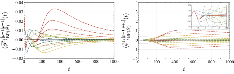
Figure 9: Borel–Padé transformation $\expectationvalue{\bar{\phi}^{2}}_{\mathrm{BP}(\bar{N})}^{[p-1|p+1]}(t)$ (left) and $\expectationvalue{\bar{\phi}^{4}}_{\mathrm{BP}(\bar{N})}^{[p-1|p+1]}(t)$ (right) for $V=\lambda\phi^{4}/4$ with $\bar{N}$ being the expansion parameter. The orders are $p=1,\,\dots,\,30$ and $p$ increases from blue to red.

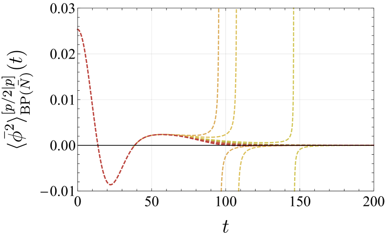
(a) $V(\phi)=\lambda\phi^{4}/4$.

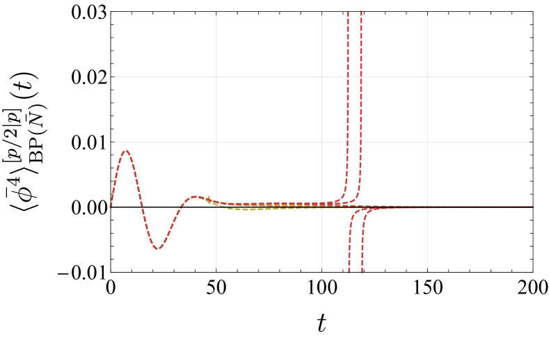
(b) $V(\phi)=\lambda\phi^{4}/4$.

Figure 10: Borel–Padé transformation $\expectationvalue{\bar{\phi}^{2}}_{\mathrm{BP}(\bar{N})}^{[p/2|p]}(t)$ (left) and $\expectationvalue{\bar{\phi}^{4}}_{\mathrm{BP}(\bar{N})}^{[p/2|p]}(t)$ (right) for $V=\lambda\phi^{4}/4$ with $\bar{N}$ being the expansion parameter. The orders are $p=16,\,18,\,\dots,\,30$ and $p$ increases from blue to red.

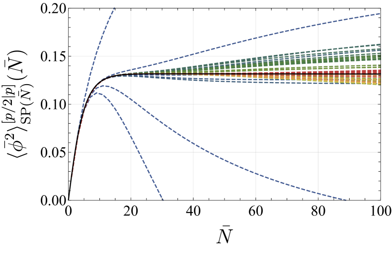
(a) $V(\phi)=\lambda\phi^{4}/4$.

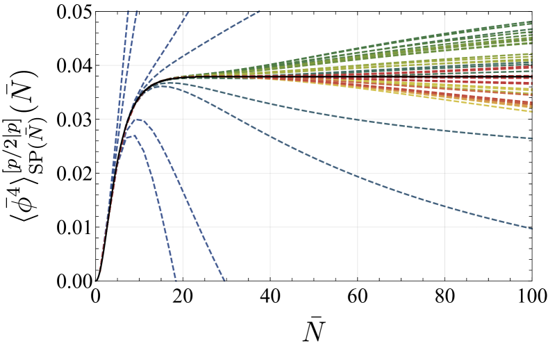
(b) $V(\phi)=\lambda\phi^{4}/4$.

Figure 11: Borel–Padé summation $\expectationvalue{\bar{\phi}^{2}}_{\mathrm{SP}(\bar{N})}^{[p/2|p]}(\bar{N})$ (left) and $\expectationvalue{\bar{\phi}^{4}}_{\mathrm{SP}(\bar{N})}^{[p/2|p]}(\bar{N})$ (right) for $V=\lambda\phi^{4}/4$ with $\bar{N}$ being the expansion parameter. The orders are $p=2,\,4,\,\dots,\,100$ and $p$ increases from blue to red.

Appendix B Numerical precision in Borel–Padé transformation

As mentioned in Sec. 3.4, special care is needed when identifying the location of the poles and zeros in the Borel plane. Figure 12 shows how the location of the poles and zeros change depending on the numerical precision. Note that the plot range is totally different from the main text: Figure 12 corresponds to a zoom-in of Fig. 7 around the origin, calculated with different numerical precisions. In this figure, the order of the Borel–Padé transformation is fixed to $p=200$, and the precision is changed as $100$, $200$, and $300$ from left to right. For precision below some threshold, poles and zeros start to appear along the circle of convergence $\absolutevalue{t}=\absolutevalue{t_{0}}\simeq 80$. These poles and zeros appear in pairs at the same locations, and they are called zero-pole ghost pairs yamada2014numerical (see also a recent progress Costin:2022hgc ). This property helps to identify them as numerical artifacts, and indeed they disappear as the precision increases.

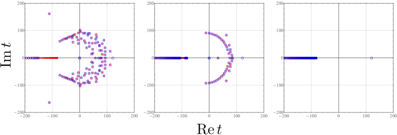
Figure 12: Precision dependence of the distribution of the poles and zeros in the Borel–Padé transformation $\expectationvalue{\bar{\phi}^{2}}_{\mathrm{BP}(\bar{N}^{2})}^{[p-1|p+1]}(t)$ (top) and $\expectationvalue{\bar{\phi}^{4}}_{\mathrm{BP}(\bar{N}^{2})}^{[p-1|p+1]}(t)$ (bottom) for $V=\lambda\phi^{4}/4$. In all the panels, the order $p$ of the Borel–Padé transformation is fixed to $p=200$, and the numerical precision is changed as $100$ (left), $200$ (middle), and $300$ (right). The cluster along the horizontal axis implies a branch cut (with the poles and zeros appearing alternately), while the one along the circle for lower precisions indicates ghost pairs (with the poles and zeros appearing at the same locations).

References

- (1) K. Sato, First-order phase transition of a vacuum and the expansion of the Universe, Monthly Notices of the Royal Astronomical Society 195 (1981) 467.
- (2) A.H. Guth, Inflationary universe: A possible solution to the horizon and flatness problems, Phys. Rev. D 23 (1981) 347.
- (3) A.A. Starobinsky, A New Type of Isotropic Cosmological Models Without Singularity, Phys. Lett. B 91 (1980) 99.
- (4) A.D. Linde, A New Inflationary Universe Scenario: A Possible Solution of the Horizon, Flatness, Homogeneity, Isotropy and Primordial Monopole Problems, Phys. Lett. B 108 (1982) 389.
- (5) A. Albrecht and P.J. Steinhardt, Cosmology for grand unified theories with radiatively induced symmetry breaking, Phys. Rev. Lett. 48 (1982) 1220.
- (6) A.D. Linde, Chaotic Inflation, Phys. Lett. B 129 (1983) 177.
- (7) Planck Collaboration, Aghanim, N., Akrami, Y., Ashdown, M., Aumont, J., Baccigalupi, C. et al., Planck 2018 results - vi. cosmological parameters, A&A 641 (2020) A6.
- (8) Planck Collaboration, Akrami, Y., Arroja, F., Ashdown, M., Aumont, J., Baccigalupi, C. et al., Planck 2018 results - x. constraints on inflation, A&A 641 (2020) A10.
- (9) Y.B. Zel’dovich and I.D. Novikov, The Hypothesis of Cores Retarded during Expansion and the Hot Cosmological Model, Soviet Ast. 10 (1967) 602.
- (10) S. Hawking, Gravitationally Collapsed Objects of Very Low Mass, Monthly Notices of the Royal Astronomical Society 152 (1971) 75 [https://academic.oup.com/mnras/article-pdf/152/1/75/9360899/mnras152-0075.pdf].
- (11) B.J. Carr and S.W. Hawking, Black Holes in the Early Universe, Monthly Notices of the Royal Astronomical Society 168 (1974) 399 [https://academic.oup.com/mnras/article-pdf/168/2/399/8079885/mnras168-0399.pdf].
- (12) B.J. Carr, The primordial black hole mass spectrum., ApJ 201 (1975) 1.
- (13) J. Kristiano and J. Yokoyama, Ruling Out Primordial Black Hole Formation From Single-Field Inflation, 2211.03395.
- (14) J. Kristiano and J. Yokoyama, Response to criticism on ”Ruling Out Primordial Black Hole Formation From Single-Field Inflation”: A note on bispectrum and one-loop correction in single-field inflation with primordial black hole formation, 2303.00341.
- (15) A. Riotto, The Primordial Black Hole Formation from Single-Field Inflation is Not Ruled Out, 2301.00599.
- (16) A. Riotto, The Primordial Black Hole Formation from Single-Field Inflation is Still Not Ruled Out, 2303.01727.
- (17) K. Ando and V. Vennin, Power spectrum in stochastic inflation, Journal of Cosmology and Astroparticle Physics 2021 (2021) 057.
- (18) K. Inomata, M. Braglia and X. Chen, Questions on calculation of primordial power spectrum with large spikes: the resonance model case, 2211.02586.
- (19) S. Choudhury, M.R. Gangopadhyay and M. Sami, No-go for the formation of heavy mass Primordial Black Holes in Single Field Inflation, 2301.10000.
- (20) S. Choudhury, S. Panda and M. Sami, No-go for PBH formation in EFT of single field inflation, 2302.05655.
- (21) S. Choudhury, S. Panda and M. Sami, Quantum loop effects on the power spectrum and constraints on primordial black holes, 2303.06066.
- (22) H. Firouzjahi, One-loop Corrections in Power Spectrum in Single Field Inflation, 2303.12025.
- (23) H. Motohashi and Y. Tada, Squeezed bispectrum and one-loop corrections in transient constant-roll inflation, 2303.16035.
- (24) A.A. Starobinsky, STOCHASTIC DE SITTER (INFLATIONARY) STAGE IN THE EARLY UNIVERSE, Lect. Notes Phys. 246 (1986) 107.
- (25) C. Pattison, V. Vennin, H. Assadullahi and D. Wands, Quantum diffusion during inflation and primordial black holes, Journal of Cosmology and Astroparticle Physics 2017 (2017) 046.
- (26) C. Pattison, V. Vennin, D. Wands and H. Assadullahi, Ultra-slow-roll inflation with quantum diffusion, Journal of Cosmology and Astroparticle Physics 2021 (2021) 080.
- (27) V. Vennin, Stochastic inflation and primordial black holes, Ph.D. thesis, U. Paris-Saclay, 6, 2020. 2009.08715.
- (28) J.M. Ezquiaga, J. García-Bellido and V. Vennin, The exponential tail of inflationary fluctuations: consequences for primordial black holes, Journal of Cosmology and Astroparticle Physics 2020 (2020) 029.
- (29) D.G. Figueroa, S. Raatikainen, S. Räsänen and E. Tomberg, Non-gaussian tail of the curvature perturbation in stochastic ultraslow-roll inflation: Implications for primordial black hole production, Phys. Rev. Lett. 127 (2021) 101302.
- (30) A. Achucarro, S. Cespedes, A.-C. Davis and G.A. Palma, The hand-made tail: non-perturbative tails from multifield inflation, JHEP 05 (2022) 052 [2112.14712].
- (31) G. Domènech, Scalar Induced Gravitational Waves Review, Universe 7 (2021) 398 [2109.01398].
- (32) A. Kogut, M.H. Abitbol, J. Chluba, J. Delabrouille, D. Fixsen, J.C. Hill et al., CMB Spectral Distortions: Status and Prospects, 1907.13195.
- (33) A. Starobinsky, Dynamics of phase transition in the new inflationary universe scenario and generation of perturbations, Physics Letters B 117 (1982) 175 .
- (34) Y. Nambu and M. Sasaki, Stochastic stage of an inflationary universe model, Physics Letters B 205 (1988) 441 .
- (35) Y. Nambu and M. Sasaki, Stochastic approach to chaotic inflation and the distribution of universes, Physics Letters B 219 (1989) 240 .
- (36) H.E. Kandrup, STOCHASTIC INFLATION AS A TIME DEPENDENT RANDOM WALK, Phys. Rev. D 39 (1989) 2245.
- (37) K.-i. Nakao, Y. Nambu and M. Sasaki, Stochastic Dynamics of New Inflation, Prog. Theor. Phys. 80 (1988) 1041.
- (38) Y. Nambu, Stochastic Dynamics of an Inflationary Model and Initial Distribution of Universes, Prog. Theor. Phys. 81 (1989) 1037.
- (39) S. Mollerach, S. Matarrese, A. Ortolan and F. Lucchin, Stochastic inflation in a simple two field model, Phys. Rev. D 44 (1991) 1670.
- (40) A.D. Linde, D.A. Linde and A. Mezhlumian, From the Big Bang theory to the theory of a stationary universe, Phys. Rev. D 49 (1994) 1783 [gr-qc/9306035].
- (41) A.A. Starobinsky and J. Yokoyama, Equilibrium state of a selfinteracting scalar field in the De Sitter background, Phys. Rev. D50 (1994) 6357 [astro-ph/9407016].
- (42) T. Prokopec, N. Tsamis and R. Woodard, Stochastic Inflationary Scalar Electrodynamics, Annals Phys. 323 (2008) 1324 [0707.0847].
- (43) F. Finelli, G. Marozzi, A.A. Starobinsky, G.P. Vacca and G. Venturi, Generation of fluctuations during inflation: Comparison of stochastic and field-theoretic approaches, Phys. Rev. D 79 (2009) 044007 [0808.1786].
- (44) F. Finelli, G. Marozzi, A. Starobinsky, G. Vacca and G. Venturi, Stochastic growth of quantum fluctuations during slow-roll inflation, Phys. Rev. D 82 (2010) 064020 [1003.1327].
- (45) B. Garbrecht, G. Rigopoulos and Y. Zhu, Infrared correlations in de Sitter space: Field theoretic versus stochastic approach, Phys. Rev. D 89 (2014) 063506 [1310.0367].
- (46) B. Garbrecht, F. Gautier, G. Rigopoulos and Y. Zhu, Feynman Diagrams for Stochastic Inflation and Quantum Field Theory in de Sitter Space, Phys. Rev. D 91 (2015) 063520 [1412.4893].
- (47) V. Onemli, Vacuum Fluctuations of a Scalar Field during Inflation: Quantum versus Stochastic Analysis, Phys. Rev. D 91 (2015) 103537 [1501.05852].
- (48) G. Cho, C.H. Kim and H. Kitamoto, Stochastic Dynamics of Infrared Fluctuations in Accelerating Universe, in 2nd LeCosPA Symposium: Everything about Gravity, Celebrating the Centenary of Einstein’s General Relativity, pp. 162–167, 2017, DOI [1508.07877].
- (49) L. Pinol, S. Renaux-Petel and Y. Tada, Inflationary stochastic anomalies, Class. Quant. Grav. 36 (2019) 07LT01 [1806.10126].
- (50) L. Pinol, S. Renaux-Petel and Y. Tada, A manifestly covariant theory of multifield stochastic inflation in phase space: solving the discretisation ambiguity in stochastic inflation, JCAP 04 (2021) 048 [2008.07497].
- (51) D. Seery, One-loop corrections to a scalar field during inflation, JCAP 11 (2007) 025 [0707.3377].
- (52) K. Enqvist, S. Nurmi, D. Podolsky and G. Rigopoulos, On the divergences of inflationary superhorizon perturbations, JCAP 04 (2008) 025 [0802.0395].
- (53) D. Seery, A parton picture of de Sitter space during slow-roll inflation, J. Cosmology Astropart. Phys. 2009 (2009) 021 [0903.2788].
- (54) C. Burgess, L. Leblond, R. Holman and S. Shandera, Super-Hubble de Sitter Fluctuations and the Dynamical RG, JCAP 03 (2010) 033 [0912.1608].
- (55) D. Seery, Infrared effects in inflationary correlation functions, Class. Quant. Grav. 27 (2010) 124005 [1005.1649].
- (56) F. Gautier and J. Serreau, Infrared dynamics in de Sitter space from Schwinger-Dyson equations, Phys. Lett. B 727 (2013) 541 [1305.5705].
- (57) M. Guilleux and J. Serreau, Quantum scalar fields in de Sitter space from the nonperturbative renormalization group, Phys. Rev. D 92 (2015) 084010 [1506.06183].
- (58) F. Gautier and J. Serreau, Scalar field correlator in de Sitter space at next-to-leading order in a 1/N expansion, Phys. Rev. D 92 (2015) 105035 [1509.05546].
- (59) R.J. Hardwick, V. Vennin, C.T. Byrnes, J. Torrado and D. Wands, The stochastic spectator, JCAP 10 (2017) 018 [1701.06473].
- (60) T. Markkanen, Renormalization of the inflationary perturbations revisited, JCAP 05 (2018) 001 [1712.02372].
- (61) D. López Nacir, F.D. Mazzitelli and L.G. Trombetta, To the sphere and back again: de Sitter infrared correlators at NTLO in 1/N, JHEP 08 (2019) 052 [1905.03665].
- (62) V. Gorbenko and L. Senatore, in dS, 1911.00022.
- (63) M. Mirbabayi, Infrared dynamics of a light scalar field in de Sitter, 1911.00564.
- (64) P. Adshead, L. Pearce, J. Shelton and Z.J. Weiner, Stochastic evolution of scalar fields with continuous symmetries during inflation, Phys. Rev. D 102 (2020) 023526 [2002.07201].
- (65) G. Moreau, J. Serreau and C. Noûs, The expansion for stochastic fields in de Sitter spacetime, 2004.09157.
- (66) T. Cohen and D. Green, Soft de Sitter Effective Theory, 2007.03693.
- (67) D.S. Salopek and J.R. Bond, Nonlinear evolution of long wavelength metric fluctuations in inflationary models, Phys. Rev. D42 (1990) 3936.
- (68) M. Sasaki and E.D. Stewart, A General analytic formula for the spectral index of the density perturbations produced during inflation, Prog. Theor. Phys. 95 (1996) 71 [astro-ph/9507001].
- (69) M. Sasaki and T. Tanaka, Super-horizon scale dynamics of multi-scalar inflation, Prog. Theor. Phys. 99 (1998) 763 [gr-qc/9801017].
- (70) D.H. Lyth, K.A. Malik and M. Sasaki, A General proof of the conservation of the curvature perturbation, JCAP 0505 (2005) 004 [astro-ph/0411220].
- (71) T. Fujita, M. Kawasaki, Y. Tada and T. Takesako, A new algorithm for calculating the curvature perturbations in stochastic inflation, JCAP 12 (2013) 036 [1308.4754].
- (72) T. Fujita, M. Kawasaki and Y. Tada, Non-perturbative approach for curvature perturbations in stochastic formalism, JCAP 10 (2014) 030 [1405.2187].
- (73) V. Vennin and A.A. Starobinsky, Correlation Functions in Stochastic Inflation, Eur. Phys. J. C 75 (2015) 413 [1506.04732].
- (74) M. Kawasaki and Y. Tada, Can massive primordial black holes be produced in mild waterfall hybrid inflation?, JCAP 08 (2016) 041 [1512.03515].
- (75) H. Assadullahi, H. Firouzjahi, M. Noorbala, V. Vennin and D. Wands, Multiple Fields in Stochastic Inflation, JCAP 06 (2016) 043 [1604.04502].
- (76) V. Vennin, H. Assadullahi, H. Firouzjahi, M. Noorbala and D. Wands, Critical Number of Fields in Stochastic Inflation, Phys. Rev. Lett. 118 (2017) 031301 [1604.06017].
- (77) C. Pattison, V. Vennin, H. Assadullahi and D. Wands, Quantum diffusion during inflation and primordial black holes, JCAP 10 (2017) 046 [1707.00537].
- (78) J.M. Ezquiaga and J. García-Bellido, Quantum diffusion beyond slow-roll: implications for primordial black-hole production, 1805.06731.
- (79) M. Biagetti, G. Franciolini, A. Kehagias and A. Riotto, Primordial Black Holes from Inflation and Quantum Diffusion, JCAP 07 (2018) 032 [1804.07124].
- (80) J.M. Ezquiaga, J. García-Bellido and V. Vennin, The exponential tail of inflationary fluctuations: consequences for primordial black holes, JCAP 03 (2020) 029 [1912.05399].
- (81) G. Panagopoulos and E. Silverstein, Primordial Black Holes from non-Gaussian tails, 1906.02827.
- (82) E. Borel, Mémoire sur les séries divergentes, Annales scientifiques de l’École Normale Supérieure 3e série, 16 (1899) 9.
- (83) J. Ecalle, Un analogue des fonctions automorphes : les fonctions résurgentes, Séminaire Choquet. Initiation à l’analyse 17 (1977-1978) .
- (84) O. Costin, Asymptotics and Borel summability, Monographs and Surveys in Pure and Applied Mathematics, CRC Press, Hoboken, NJ (2008).
- (85) M. Marino, Lectures on non-perturbative effects in large N gauge theories, matrix models and strings, 1206.6272.
- (86) D. Dorigoni, An Introduction to Resurgence, Trans-Series and Alien Calculus, Annals Phys. 409 (2019) 167914 [1411.3585].
- (87) I. Aniceto, G. Başar and R. Schiappa, A primer on resurgent transseries and their asymptotics, Physics Reports 809 (2019) 1.
- (88) D. Sauzin, Introduction to 1-summability and resurgence, 1405.0356.
- (89) C.M. Bender and T.T. Wu, Anharmonic oscillator, Phys. Rev. 184 (1969) 1231.
- (90) C.M. Bender and T.T. Wu, Anharmonic oscillator. 2: A Study of perturbation theory in large order, Phys. Rev. D 7 (1973) 1620.
- (91) R. Balian, G. Parisi and A. Voros, QUARTIC OSCILLATOR, in Mathematical Problems in Feynman Path Integral, 5, 1978.
- (92) A. Voros, The return of the quartic oscillator. the complex wkb method, Annales de l’I.H.P. Physique théorique 39 (1983) 211.
- (93) J. Zinn-Justin and U.D. Jentschura, Multi-instantons and exact results I: Conjectures, WKB expansions, and instanton interactions, Annals Phys. 313 (2004) 197 [quant-ph/0501136].
- (94) J. Zinn-Justin and U.D. Jentschura, Multi-instantons and exact results II: Specific cases, higher-order effects, and numerical calculations, Annals Phys. 313 (2004) 269 [quant-ph/0501137].
- (95) U.D. Jentschura, A. Surzhykov and J. Zinn-Justin, Multi-instantons and exact results. III: Unification of even and odd anharmonic oscillators, Annals Phys. 325 (2010) 1135 [1001.3910].
- (96) U.D. Jentschura and J. Zinn-Justin, Multi-instantons and exact results. IV: Path integral formalism, Annals Phys. 326 (2011) 2186.
- (97) G.V. Dunne and M. Unsal, Generating nonperturbative physics from perturbation theory, Phys. Rev. D89 (2014) 041701 [1306.4405].
- (98) G. Basar, G.V. Dunne and M. Unsal, Resurgence theory, ghost-instantons, and analytic continuation of path integrals, JHEP 10 (2013) 041 [1308.1108].
- (99) G.V. Dunne and M. Unsal, Uniform WKB, Multi-instantons, and Resurgent Trans-Series, Phys. Rev. D89 (2014) 105009 [1401.5202].
- (100) M.A. Escobar-Ruiz, E. Shuryak and A.V. Turbiner, Three-loop Correction to the Instanton Density. I. The Quartic Double Well Potential, Phys. Rev. D 92 (2015) 025046 [1501.03993].
- (101) M.A. Escobar-Ruiz, E. Shuryak and A.V. Turbiner, Three-loop Correction to the Instanton Density. II. The Sine-Gordon potential, Phys. Rev. D 92 (2015) 025047 [1505.05115].
- (102) T. Misumi, M. Nitta and N. Sakai, Resurgence in sine-Gordon quantum mechanics: Exact agreement between multi-instantons and uniform WKB, JHEP 09 (2015) 157 [1507.00408].
- (103) A. Behtash, G.V. Dunne, T. Schäfer, T. Sulejmanpasic and M. Ünsal, Complexified path integrals, exact saddles and supersymmetry, Phys. Rev. Lett. 116 (2016) 011601 [1510.00978].
- (104) A. Behtash, G.V. Dunne, T. Schaefer, T. Sulejmanpasic and M. Unsal, Toward Picard-Lefschetz Theory of Path Integrals, Complex Saddles and Resurgence, 1510.03435.
- (105) I. Gahramanov and K. Tezgin, Remark on the Dunne-Ünsal relation in exact semiclassics, Phys. Rev. D 93 (2016) 065037 [1512.08466].
- (106) G.V. Dunne and M. Unsal, WKB and Resurgence in the Mathieu Equation, 1603.04924.
- (107) C. Kozcaz, T. Sulejmanpasic, Y. Tanizaki and M. Unsal, Cheshire Cat resurgence, Self-resurgence and Quasi-Exact Solvable Systems, 1609.06198.
- (108) T. Fujimori, S. Kamata, T. Misumi, M. Nitta and N. Sakai, Nonperturbative contributions from complexified solutions in models, Phys. Rev. D94 (2016) 105002 [1607.04205].
- (109) G.V. Dunne and M. Unsal, Deconstructing zero: resurgence, supersymmetry and complex saddles, JHEP 12 (2016) 002 [1609.05770].
- (110) M. Serone, G. Spada and G. Villadoro, Instantons from Perturbation Theory, Phys. Rev. D 96 (2017) 021701 [1612.04376].
- (111) G. Basar, G.V. Dunne and M. Unsal, Quantum Geometry of Resurgent Perturbative/Nonperturbative Relations, JHEP 05 (2017) 087 [1701.06572].
- (112) G. Álvarez and H.J. Silverstone, A new method to sum divergent power series: educated match, J. Phys. Comm. 1 (2017) 025005 [1706.00329].
- (113) A. Behtash, G.V. Dunne, T. Schaefer, T. Sulejmanpasic and M. Ünsal, Critical Points at Infinity, Non-Gaussian Saddles, and Bions, JHEP 06 (2018) 068 [1803.11533].
- (114) Z. Duan, J. Gu, Y. Hatsuda and T. Sulejmanpasic, Instantons in the Hofstadter butterfly: difference equation, resurgence and quantum mirror curves, JHEP 01 (2019) 079 [1806.11092].
- (115) M. Raman and P.N. Bala Subramanian, Chebyshev wells: Periods, deformations, and resurgence, Phys. Rev. D 101 (2020) 126014 [2002.01794].
- (116) N. Sueishi, problem in resurgence, PTEP 2021 (2021) 013B01 [1912.03518].
- (117) N. Sueishi, S. Kamata, T. Misumi and M. Ünsal, On exact-WKB analysis, resurgent structure, and quantization conditions, JHEP 12 (2020) 114 [2008.00379].
- (118) N. Sueishi, S. Kamata, T. Misumi and M. Ünsal, Exact-WKB, complete resurgent structure, and mixed anomaly in quantum mechanics on , 2103.06586.
- (119) I. Aniceto and M. Spaliński, Resurgence in Extended Hydrodynamics, Phys. Rev. D 93 (2016) 085008 [1511.06358].
- (120) G. Basar and G.V. Dunne, Hydrodynamics, resurgence, and transasymptotics, Phys. Rev. D 92 (2015) 125011 [1509.05046].
- (121) J. Casalderrey-Solana, N.I. Gushterov and B. Meiring, Resurgence and Hydrodynamic Attractors in Gauss-Bonnet Holography, JHEP 04 (2018) 042 [1712.02772].
- (122) A. Behtash, C.N. Cruz-Camacho and M. Martinez, Far-from-equilibrium attractors and nonlinear dynamical systems approach to the Gubser flow, Phys. Rev. D 97 (2018) 044041 [1711.01745].
- (123) M.P. Heller and V. Svensson, How does relativistic kinetic theory remember about initial conditions?, Phys. Rev. D 98 (2018) 054016 [1802.08225].
- (124) M.P. Heller, A. Serantes, M. Spaliński, V. Svensson and B. Withers, The hydrodynamic gradient expansion in linear response theory, 2007.05524.
- (125) I. Aniceto, B. Meiring, J. Jankowski and M. Spaliński, The large proper-time expansion of Yang-Mills plasma as a resurgent transseries, JHEP 02 (2019) 073 [1810.07130].
- (126) A. Behtash, S. Kamata, M. Martinez, T. Schäfer and V. Skokov, Transasymptotics and hydrodynamization of the Fokker-Planck equation for gluons, Phys. Rev. D 103 (2021) 056010 [2011.08235].
- (127) M. Marino, R. Schiappa and M. Weiss, Multi-Instantons and Multi-Cuts, J. Math. Phys. 50 (2009) 052301 [0809.2619].
- (128) S. Garoufalidis, A. Its, A. Kapaev and M. Marino, Asymptotics of the instantons of Painlevé I, Int. Math. Res. Not. 2012 (2012) 561 [1002.3634].
- (129) C.-T. Chan, H. Irie and C.-H. Yeh, Stokes Phenomena and Non-perturbative Completion in the Multi-cut Two-matrix Models, Nucl. Phys. B 854 (2012) 67 [1011.5745].
- (130) C.-T. Chan, H. Irie and C.-H. Yeh, Stokes Phenomena and Quantum Integrability in Non-critical String/M Theory, Nucl. Phys. B 855 (2012) 46 [1109.2598].
- (131) R. Schiappa and R. Vaz, The Resurgence of Instantons: Multi-Cut Stokes Phases and the Painleve II Equation, Commun. Math. Phys. 330 (2014) 655 [1302.5138].
- (132) M. Marino, Open string amplitudes and large order behavior in topological string theory, JHEP 03 (2008) 060 [hep-th/0612127].
- (133) M. Marino, R. Schiappa and M. Weiss, Nonperturbative Effects and the Large-Order Behavior of Matrix Models and Topological Strings, Commun. Num. Theor. Phys. 2 (2008) 349 [0711.1954].
- (134) M. Marino, Nonperturbative effects and nonperturbative definitions in matrix models and topological strings, JHEP 12 (2008) 114 [0805.3033].
- (135) S. Pasquetti and R. Schiappa, Borel and Stokes Nonperturbative Phenomena in Topological String Theory and c=1 Matrix Models, Annales Henri Poincare 11 (2010) 351 [0907.4082].
- (136) I. Aniceto, R. Schiappa and M. Vonk, The Resurgence of Instantons in String Theory, Commun. Num. Theor. Phys. 6 (2012) 339 [1106.5922].
- (137) R. Couso-Santamaría, J.D. Edelstein, R. Schiappa and M. Vonk, Resurgent Transseries and the Holomorphic Anomaly, Annales Henri Poincare 17 (2016) 331 [1308.1695].
- (138) R. Couso-Santamaría, J.D. Edelstein, R. Schiappa and M. Vonk, Resurgent Transseries and the Holomorphic Anomaly: Nonperturbative Closed Strings in Local , Commun. Math. Phys. 338 (2015) 285 [1407.4821].
- (139) A. Grassi, M. Marino and S. Zakany, Resumming the string perturbation series, JHEP 05 (2015) 038 [1405.4214].
- (140) R. Couso-Santamaría, R. Schiappa and R. Vaz, Finite N from Resurgent Large N, Annals Phys. 356 (2015) 1 [1501.01007].
- (141) R. Couso-Santamaría, R. Schiappa and R. Vaz, On asymptotics and resurgent structures of enumerative Gromov–Witten invariants, Commun. Num. Theor. Phys. 11 (2017) 707 [1605.07473].
- (142) R. Couso-Santamaría, M. Marino and R. Schiappa, Resurgence Matches Quantization, J. Phys. A 50 (2017) 145402 [1610.06782].
- (143) T. Kuroki and F. Sugino, Resurgence of one-point functions in a matrix model for 2D type IIA superstrings, JHEP 05 (2019) 138 [1901.10349].
- (144) T. Kuroki, Two-point functions at arbitrary genus and its resurgence structure in a matrix model for 2D type IIA superstrings, JHEP 07 (2020) 118 [2004.13346].
- (145) D. Dorigoni and A. Kleinschmidt, Resurgent expansion of Lambert series and iterated Eisenstein integrals, Commun. Num. Theor. Phys. 15 (2021) 1 [2001.11035].
- (146) G.V. Dunne and M. Unsal, Resurgence and Trans-series in Quantum Field Theory: The CP(N-1) Model, JHEP 11 (2012) 170 [1210.2423].
- (147) G.V. Dunne and M. Unsal, Continuity and Resurgence: towards a continuum definition of the (N-1) model, Phys. Rev. D87 (2013) 025015 [1210.3646].
- (148) A. Cherman, D. Dorigoni, G.V. Dunne and M. Unsal, Resurgence in Quantum Field Theory: Nonperturbative Effects in the Principal Chiral Model, Phys. Rev. Lett. 112 (2014) 021601 [1308.0127].
- (149) A. Cherman, D. Dorigoni and M. Unsal, Decoding perturbation theory using resurgence: Stokes phenomena, new saddle points and Lefschetz thimbles, JHEP 10 (2015) 056 [1403.1277].
- (150) T. Misumi, M. Nitta and N. Sakai, Neutral bions in the model, JHEP 06 (2014) 164 [1404.7225].
- (151) M. Nitta, Fractional instantons and bions in the O model with twisted boundary conditions, JHEP 03 (2015) 108 [1412.7681].
- (152) M. Nitta, Fractional instantons and bions in the principal chiral model on with twisted boundary conditions, JHEP 08 (2015) 063 [1503.06336].
- (153) A. Behtash, T. Sulejmanpasic, T. Schäfer and M. Ünsal, Hidden topological angles and Lefschetz thimbles, Phys. Rev. Lett. 115 (2015) 041601 [1502.06624].
- (154) G.V. Dunne and M. Unsal, Resurgence and Dynamics of O(N) and Grassmannian Sigma Models, JHEP 09 (2015) 199 [1505.07803].
- (155) P.V. Buividovich, G.V. Dunne and S.N. Valgushev, Complex Path Integrals and Saddles in Two-Dimensional Gauge Theory, Phys. Rev. Lett. 116 (2016) 132001 [1512.09021].
- (156) S. Demulder, D. Dorigoni and D.C. Thompson, Resurgence in -deformed Principal Chiral Models, JHEP 07 (2016) 088 [1604.07851].
- (157) T. Sulejmanpasic, Global Symmetries, Volume Independence, and Continuity in Quantum Field Theories, Phys. Rev. Lett. 118 (2017) 011601 [1610.04009].
- (158) K. Okuyama and K. Sakai, Resurgence analysis of 2d Yang-Mills theory on a torus, JHEP 08 (2018) 065 [1806.00189].
- (159) M.C. Abbott, Z. Bajnok, J. Balog, A. Hegedús and S. Sadeghian, Resurgence in the O(4) sigma model, 2011.12254.
- (160) M.C. Abbott, Z. Bajnok, J. Balog and A. Hegedús, From perturbative to non-perturbative in the O(4) sigma model, 2011.09897.
- (161) K. Ishikawa, O. Morikawa, A. Nakayama, K. Shibata, H. Suzuki and H. Takaura, Infrared renormalon in the supersymmetric model on , PTEP 2020 (2020) 023B10 [1908.00373].
- (162) K. Ishikawa, M. Okuto, K. Shibata and H. Suzuki, Vacuum energy of the supersymmetric model on in the expansion, PTEP 2020 (2020) 063B02 [2001.07302].
- (163) S. Gukov, M. Marino and P. Putrov, Resurgence in complex Chern-Simons theory, 1605.07615.
- (164) D. Gang and Y. Hatsuda, S-duality resurgence in SL(2) Chern-Simons theory, JHEP 07 (2018) 053 [1710.09994].
- (165) D.H. Wu, Resurgent analysis of SU(2) Chern-Simons partition function on Brieskorn spheres , JHEP 21 (2020) 008 [2010.13736].
- (166) H. Fuji, K. Iwaki, H. Murakami and Y. Terashima, Witten-Reshetikhin-Turaev function for a knot in Seifert manifolds, 2007.15872.
- (167) F. Ferrari and P. Putrov, Supergroups, q-series and 3-manifolds, 2009.14196.
- (168) S. Gukov and C. Manolescu, A two-variable series for knot complements, 1904.06057.
- (169) S. Garoufalidis, J. Gu and M. Marino, The resurgent structure of quantum knot invariants, 2007.10190.
- (170) P. Argyres and M. Unsal, A semiclassical realization of infrared renormalons, Phys. Rev. Lett. 109 (2012) 121601 [1204.1661].
- (171) G.V. Dunne, M. Shifman and M. Unsal, Infrared Renormalons versus Operator Product Expansions in Supersymmetric and Related Gauge Theories, Phys. Rev. Lett. 114 (2015) 191601 [1502.06680].
- (172) M. Yamazaki and K. Yonekura, From 4d Yang-Mills to 2d model: IR problem and confinement at weak coupling, JHEP 07 (2017) 088 [1704.05852].
- (173) H. Mera, T.G. Pedersen and B.K. Nikolić, Fast summation of divergent series and resurgent transseries from Meijer- G approximants, Phys. Rev. D 97 (2018) 105027 [1802.06034].
- (174) E. Itou, Fractional instanton of the SU() gauge theory in weak coupling regime, JHEP 05 (2019) 093 [1811.05708].
- (175) F. Canfora, M. Lagos, S.H. Oh, J. Oliva and A. Vera, Analytic (3+1)-dimensional gauged Skyrmions, Heun, and Whittaker-Hill equations and resurgence, Phys. Rev. D 98 (2018) 085003 [1809.10386].
- (176) M. Ashie, O. Morikawa, H. Suzuki, H. Takaura and K. Takeuchi, Infrared renormalon in QCD(adj.) on , PTEP 2020 (2020) 023B01 [1909.05489].
- (177) K. Ishikawa, O. Morikawa, K. Shibata, H. Suzuki and H. Takaura, Renormalon structure in compactified spacetime, PTEP 2020 (2020) 013B01 [1909.09579].
- (178) M. Ünsal, Strongly coupled QFT dynamics via TQFT coupling, 2007.03880.
- (179) M. Ashie, O. Morikawa, H. Suzuki and H. Takaura, More on the infrared renormalon in U(N) QCD(adj.) on , PTEP 2020 (2020) 093B02 [2005.07407].
- (180) O. Morikawa and H. Takaura, Identification of perturbative ambiguity canceled against bion, Phys. Lett. B 807 (2020) 135570 [2003.04759].
- (181) J.G. Russo, A Note on perturbation series in supersymmetric gauge theories, JHEP 06 (2012) 038 [1203.5061].
- (182) I. Aniceto, J.G. Russo and R. Schiappa, Resurgent Analysis of Localizable Observables in Supersymmetric Gauge Theories, JHEP 03 (2015) 172 [1410.5834].
- (183) I. Aniceto, The Resurgence of the Cusp Anomalous Dimension, J. Phys. A 49 (2016) 065403 [1506.03388].
- (184) M. Honda, Borel Summability of Perturbative Series in 4D and 5D =1 Supersymmetric Theories, Phys. Rev. Lett. 116 (2016) 211601 [1603.06207].
- (185) M. Honda, How to resum perturbative series in 3d N=2 Chern-Simons matter theories, Phys. Rev. D94 (2016) 025039 [1604.08653].
- (186) S. Gukov, RG Flows and Bifurcations, Nucl. Phys. B 919 (2017) 583 [1608.06638].
- (187) M. Honda, Role of Complexified Supersymmetric Solutions, 1710.05010.
- (188) S. Gukov, D. Pei, P. Putrov and C. Vafa, BPS spectra and 3-manifold invariants, J. Knot Theor. Ramifications 29 (2020) 2040003 [1701.06567].
- (189) D. Dorigoni and P. Glass, The grin of Cheshire cat resurgence from supersymmetric localization, SciPost Phys. 4 (2018) 012 [1711.04802].
- (190) M. Honda and D. Yokoyama, Resumming perturbative series in the presence of monopole bubbling effects, Phys. Rev. D 100 (2019) 025012 [1711.10799].
- (191) T. Fujimori, M. Honda, S. Kamata, T. Misumi and N. Sakai, Resurgence and Lefschetz thimble in three-dimensional supersymmetric Chern–Simons matter theories, PTEP 2018 (2018) 123B03 [1805.12137].
- (192) A. Grassi, J. Gu and M. Mariño, Non-perturbative approaches to the quantum Seiberg-Witten curve, JHEP 07 (2020) 106 [1908.07065].
- (193) D. Dorigoni and P. Glass, Picard-Lefschetz decomposition and Cheshire Cat resurgence in 3D = 2 field theories, JHEP 12 (2019) 085 [1909.05262].
- (194) D. Dorigoni, M.B. Green and C. Wen, Exact properties of an integrated correlator in SYM, 2102.09537.
- (195) T. Fujimori, M. Honda, S. Kamata, T. Misumi, N. Sakai and T. Yoda, Quantum phase transition and resurgence: Lessons from three-dimensional supersymmetric quantum electrodynamics, PTEP 2021 (2021) 103B04 [2103.13654].
- (196) Y. Hatsuda and M. Kimura, Spectral Problems for Quasinormal Modes of Black Holes, Universe 7 (2021) 476 [2111.15197].
- (197) Y. Hatsuda, Quasinormal modes of black holes and Borel summation, Phys. Rev. D 101 (2020) 024008 [1906.07232].
- (198) J. Matyjasek and M. Telecka, Quasinormal modes of black holes. II. Padé summation of the higher-order WKB terms, Phys. Rev. D 100 (2019) 124006 [1908.09389].
- (199) D.S. Eniceicu and M. Reece, Quasinormal modes of charged fields in Reissner-Nordström backgrounds by Borel-Padé summation of Bender-Wu series, Phys. Rev. D 102 (2020) 044015 [1912.05553].
- (200) D. Polarski and A.A. Starobinsky, Semiclassicality and decoherence of cosmological perturbations, Class. Quant. Grav. 13 (1996) 377 [gr-qc/9504030].
- (201) J. Lesgourgues, D. Polarski and A.A. Starobinsky, Quantum to classical transition of cosmological perturbations for nonvacuum initial states, Nucl. Phys. B 497 (1997) 479 [gr-qc/9611019].
- (202) D. Polarski, Classicality of primordial fluctuations and primordial black holes, Int. J. Mod. Phys. D 10 (2001) 927 [astro-ph/0109388].
- (203) C. Kiefer and D. Polarski, Why do cosmological perturbations look classical to us?, Adv. Sci. Lett. 2 (2009) 164 [0810.0087].
- (204) C.P. Burgess, R. Holman, G. Tasinato and M. Williams, EFT Beyond the Horizon: Stochastic Inflation and How Primordial Quantum Fluctuations Go Classical, JHEP 03 (2015) 090 [1408.5002].
- (205) J. Martin and V. Vennin, Quantum Discord of Cosmic Inflation: Can we Show that CMB Anisotropies are of Quantum-Mechanical Origin?, Phys. Rev. D 93 (2016) 023505 [1510.04038].
- (206) M. Morikawa, Dissipation and Fluctuation of Quantum Fields in Expanding Universes, Phys. Rev. D42 (1990) 1027.
- (207) E.A. Calzetta, B.L. Hu and F.D. Mazzitelli, Coarse grained effective action and renormalization group theory in semiclassical gravity and cosmology, Phys. Rept. 352 (2001) 459 [hep-th/0102199].
- (208) S. Matarrese, M.A. Musso and A. Riotto, Influence of superhorizon scales on cosmological observables generated during inflation, JCAP 0405 (2004) 008 [hep-th/0311059].
- (209) L. Perreault Levasseur, Lagrangian formulation of stochastic inflation: Langevin equations, one-loop corrections and a proposed recursive approach, Phys. Rev. D88 (2013) 083537 [1304.6408].
- (210) I. Moss and G. Rigopoulos, Effective long wavelength scalar dynamics in de Sitter, JCAP 1705 (2017) 009 [1611.07589].
- (211) J. Tokuda and T. Tanaka, Statistical nature of infrared dynamics on de Sitter background, JCAP 02 (2018) 014 [1708.01734].
- (212) T. Prokopec and G. Rigopoulos, Functional renormalization group for stochastic inflation, JCAP 08 (2018) 013 [1710.07333].
- (213) K. Enqvist, R.N. Lerner, O. Taanila and A. Tranberg, Spectator field dynamics in de Sitter and curvaton initial conditions, JCAP 10 (2012) 052 [1205.5446].
- (214) S. Winitzki and A. Vilenkin, Effective noise in stochastic description of inflation, Phys. Rev. D61 (2000) 084008 [gr-qc/9911029].
- (215) M. Liguori, S. Matarrese, M. Musso and A. Riotto, Stochastic inflation and the lower multipoles in the CMB anisotropies, JCAP 0408 (2004) 011 [astro-ph/0405544].
- (216) S. Habib, Stochastic inflation: The Quantum phase space approach, Phys. Rev. D 46 (1992) 2408 [gr-qc/9208006].
- (217) J. Grain and V. Vennin, Stochastic inflation in phase space: Is slow roll a stochastic attractor?, JCAP 05 (2017) 045 [1703.00447].
- (218) G. Ballesteros, J. Rey, M. Taoso and A. Urbano, Stochastic inflationary dynamics beyond slow-roll and consequences for primordial black hole formation, JCAP 08 (2020) 043 [2006.14597].
- (219) A.A. Starobinsky and J. Yokoyama, Equilibrium state of a self-interacting scalar field in the de sitter background, Phys. Rev. D 50 (1994) 6357.
- (220) N. Tsamis and R. Woodard, Stochastic quantum gravitational inflation, Nuclear Physics B 724 (2005) 295.
- (221) F. Finelli, G. Marozzi, A.A. Starobinsky, G.P. Vacca and G. Venturi, Generation of fluctuations during inflation: Comparison of stochastic and field-theoretic approaches, Phys. Rev. D 79 (2009) 044007.
- (222) E.O. Kahya and V.K. Onemli, Quantum stability of a phase of cosmic acceleration, Phys. Rev. D 76 (2007) 043512.
- (223) G. Baker, G. Baker, P. Graves-Morris and S. Baker, Pade Approximants: Encyclopedia of Mathematics and It’s Applications, Vol. 59 George A. Baker, Jr., Peter Graves-Morris, Encyclopedia of Mathematics and its Applications, Cambridge University Press (1996).
- (224) H.S. Yamada and K.S. Ikeda, A numerical test of pade approximation for some functions with singularity, 1308.4453.
- (225) A. Sen, S-duality Improved Superstring Perturbation Theory, JHEP 11 (2013) 029 [1304.0458].
- (226) C. Beem, L. Rastelli, A. Sen and B.C. van Rees, Resummation and S-duality in N=4 SYM, JHEP 04 (2014) 122 [1306.3228].
- (227) M. Honda, On Perturbation theory improved by Strong coupling expansion, JHEP 12 (2014) 019 [1408.2960].
- (228) M. Honda and D.P. Jatkar, Interpolating function and Stokes Phenomena, Nucl. Phys. B 900 (2015) 533 [1504.02276].
- (229) L.F. Alday and A. Bissi, Modular interpolating functions for N=4 SYM, JHEP 07 (2014) 007 [1311.3215].
- (230) A. Chowdhury, M. Honda and S. Thakur, S-duality invariant perturbation theory improved by holography, JHEP 04 (2017) 137 [1607.01716].
- (231) O. Costin and G.V. Dunne, Physical Resurgent Extrapolation, Phys. Lett. B 808 (2020) 135627 [2003.07451].
- (232) O. Costin and G.V. Dunne, Uniformization and Constructive Analytic Continuation of Taylor Series, 2009.01962.
- (233) O. Costin and G.V. Dunne, Conformal and uniformizing maps in Borel analysis, Eur. Phys. J. ST 230 (2021) 2679 [2108.01145].
- (234) O. Costin, G.V. Dunne and M. Meynig, Noise effects on Padé approximants and conformal maps ∗, J. Phys. A 55 (2022) 464007 [2208.02410].
- (235) C.M. Bender and S.A. Orszag, Advanced Mathematical Methods for Scientists and Engineers, McGraw-Hill (1978).
- (236) T. Kawai and Y. Takei, Algebraic analysis of singular perturbation theory * (translations of mathematical monographs 227) * by takahiro kawai and yoshitsugu takei (translated by goro kato): * 130 pp., us$29.00 isbn 0-8218-3547-5 * (american mathematical society, providence, ri, 2005), .
- (237) I.S. Gradshteyn, I.M. Ryzhik, D. Zwillinger and V. Moll, Table of integrals, series, and products; 8th ed., Academic Press, Amsterdam (2015), 0123849330.