Higher genus meanders and Masur–Veech volumes

Abstract.

A classical meander is a pair consisting of a straight line in the plane and of a smooth closed curve transversally intersecting the line, where the pair is considered up to an isotopy preserving the straight line. The number $\operatorname{M}(N)$ of meanders with $2N$ intersections grows exponentially with $N$, but asymptotics still remains conjectural.

A meander defines a pair of transversally intersecting simple closed curves on a 2-sphere. In this paper we consider pairs of transversally intersecting simple closed curves on a closed oriented surface of arbitrary genus $g$. The number of such higher genus meanders still admits exponential upper and lower bounds as the number of intersections grows. Fixing the number $n$ of bigons in the complement to the union of the two curves, we compute the precise asymptotics of genus $g$ meanders with $n$ bigons and with at most $2N$ intersections and show that this asymptotics is polynomial in $N$ as $N\to\infty$. We obtain a similar result for the number of positively intersecting pairs of oriented simple closed curves on a surface of genus $g$. We also compute the asymptotic probability of getting a meander from a random braid on a surface of genus $g-1$ with two boundary components.

In order to effectively count meanders we identify them with integer points represented by certain square-tiled surfaces in the moduli spaces of Abelian and quadratic differentials and make use of recent advances in the geometry of these moduli spaces combined with asymptotic properties of Witten–Kontsevich $2$-correlators on moduli spaces of complex curves.

1. Introduction

1.1. Classical meanders

A meander is a topological configuration of an oriented straight line in the plane and of a smooth simple closed curve intersecting transversally the straight line considered up to an isotopy of the plane preserving the straight line. Meanders can be traced back to H. Poincaré [Po] and naturally appear in various areas of mathematics, theoretical physics and computational biology (in particular, they provide a model of polymer folding [DiGG1]).

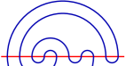
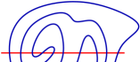
Figure 1. Equivalent meanders with 10 crossings

The asymptotic count of the number $\operatorname{M}(N)$ of meanders with exactly $2N$ crossings as $N$ tends to infinity is one of the oldest open questions in the study of meanders. The problem was popularized by V. I. Arnold (see Problem 1986-7 in [Arn] and later comments by M. Kontsevich and S. Lando in the same book). Exponential upper and lower bounds for this number were obtained by S. Lando and A. Zvonkin in [LZv1] and in [LZv2]. They conjectured that there exist constants $const,R,\alpha$ such that

(1.1) $$\operatorname{M}(N)\overset{?}{\sim}const\cdot R^{2N}\cdot N^{\alpha}\quad\text{as}\quad N\to\infty\,.$$

The conjecture was sharpened by P. Di Francesco, O. Golinelli, E. Guitter [DiGG1], [DiGG2], who described the generating function of meandric numbers $\operatorname{M}(N)$. They suggested in [DiGG2] a conjectural exact value $\alpha=-\frac{29+\sqrt{145}}{12}\approx-3.42$ interpreted as the corresponding critical exponent $\alpha$ in a two-dimensional conformal field theory with central charge $c=-4$ coupled to gravity. The conjectural approximate value $R^{2}\approx 12.26$ was suggested by I. Jensen [Jen] through computer simulations. The best known rigorous bounds for the constant $R^{2}$ are $11.380\leq R^{2}\leq 12.901$, as proved in [AlP]. However, all elements of this conjecture stated thirty years ago are still open.

Mathematical literature devoted to meanders is vast and varies from representation theory, see [DeKi], [DuYu], [ElJ], [D], and theory of PDEs [FiRo] to theoretical physics [DiDGG] and more recently to Schramm–Loewner evolution curves on a Liouville quantum gravity surface [BGS]. Meanders are particular cases of more general meandric systems, recently studied in [CuKST], [FeT] [FuNe], [GnNP], [Kg]. We recommend a beautiful recent survey [Zv] on meanders for further details and references.

One can organize meanders into groups and count them group by group. For example, one can fix the number $n$ of minimal arcs (marked by black color in Figure 2) and count separately the number $\operatorname{M}^{+}_{0,n}(N)$ (respectively $\operatorname{M}^{-}_{0,n}(N)$) of meanders with at most $2N$ crossings, exactly $n$ minimal arcs and having (respectively not having) a maximal arc.

Figure 2. Meanders with and without maximal arcs. Both meanders have $5$ minimal arcs.

We proved in [DGZZ2] that the counting functions $\operatorname{M}^{+}_{0,n}(N)$ and $\operatorname{M}^{-}_{0,n}(N)$ admit the following asymptotics as $N\to+\infty$:

$$\operatorname{M}^{+}_{0,n}(N) =\frac{2}{n!\,(n-3)!}\left(\frac{2}{\pi^{2}}\right)^{n-2}\cdot\binom{2n-2}{n-1}^{2}\cdot\frac{N^{2n-4}}{4n-8}\ +\ o(N^{2n-4})\,.$$

$$\operatorname{M}^{-}_{0,n}(N) =\frac{4}{n!\,(n-4)!}\left(\frac{2}{\pi^{2}}\right)^{n-3}\cdot\binom{2n-4}{n-2}^{2}\cdot\frac{N^{2n-5}}{4n-10}\ +\ o(N^{2n-5})\,.$$

This restricted count giving polynomial asymptotics for $\operatorname{M}^{\pm}_{0,n}(N)$ versus exponential asymptotics for $\operatorname{M}(N)$ neither contradicts nor corroborates conjecture (1.1). A meander with $2N$ crossings can have from $3$ to $2N-1$ minimal arcs, so $\operatorname{M}(N)=\sum_{n=3}^{2N-1}\operatorname{M}^{+}_{0,n}(N)+\sum_{n=4}^{2N-2}\operatorname{M}^{-}_{0,n}(N)$. However, the sum of asymptotic expressions on the right-hand sides of the above formulas for $\operatorname{M}^{\pm}_{0,n}$ has no relation to $\operatorname{M}(N)$. The problem is that, conjecturally, roughly half of the arcs of a typical meander with large number of crossings are minimal, while in the asymptotic formulas for $\operatorname{M}^{\pm}_{0,n}(N)$ we fix $n$ and only then let $N\to+\infty$, so our asymptotic formulas make sense only in the regime when $n\ll N$.

Meanders with a fixed number $n$ of minimal arcs are related to simple closed geodesics on a hyperbolic sphere with $n$ cusps. When the number of intersections $2N$ is large, this number gives a reasonable approximation of the length of a simple closed geodesic in this correspondence. M. Mirzakhani proved in [Mi2] that the number of simple closed hyperbolic geodesics of bounded length $L$ has exact polynomial asymptotics with respect to $L$, while, by classical results of Delsarte, Huber and Selberg, the total number of closed geodesics of length bounded by $L$ grows exponentially as $e^{L}/L$.

1.2. Higher genus meanders

Meanders can be considered as configurations of ordered pairs of simple closed curves on a 2-sphere, where the first curve, corresponding to the straight line, is endowed with a marked point distinct from intersection points with the second curve. Applying an appropriate diffeomorphism of the sphere we can send the first curve to a large circle on a round sphere; postcomposing this diffeomorphism with the stereographic projection from the marked point to the plane we get a classical meander.

In this paper, we count higher genus meanders represented by ordered pairs of transversally intersecting smooth simple closed curves on a higher genus surface. As before, two pairs are considered as equivalent if there exists an orientation preserving diffeomorphism of the surface (not necessarily homotopic to identity) which sends one ordered pair of curves to another pair respecting the ordering of curves. We do not distinguish any point of the first curve in the higher genus case.

Denote by $\mathcal{G}$ be the embedded graph defined by a transverse pair of multicurves on a surface $S$. Vertices of $\mathcal{G}$ are the intersection points of the pair of multicurves. The boundary components of the complement $S-\mathcal{G}$ correspond to closed broken lines formed by edges of $\mathcal{G}$.

Definition 1.1.

The boundary components of the complement $S-\mathcal{G}$ formed by two edges of $\mathcal{G}$ are called bigons. A bigon is called filling when it bounds a topological disc and non-filling otherwise.

In the genus zero case, bigons correspond to minimal arcs and are always filling. In higher genera a bigon might bound a connected component of $S-\mathcal{G}$ having nontrivial topology; it can also represent just one of several boundary components of a connected component of $S-\mathcal{G}$. However, we will see in Section 4 that when the number of bigons is fixed, while the number of intersections grows, for all but a vanishing part (as $N\to+\infty$) of meanders all bigons are filling, and, more generally, for most of meanders all connected components of $S-\mathcal{G}$ are topological discs.

We count higher genus meanders in two settings. In the first setting we study asymptotics of the number $\operatorname{M}_{g,n}(N)$ of meanders with exactly $n$ bigons (generalizing minimal arcs) on a surface of genus $g$ with at most $2N$ crossings, as the bound $2N$ for the number of crossings tends to infinity.

In the second setting we study asymptotics of the number $\operatorname{M}^{+}_{g}(N)$ of oriented meanders, for which the curves are oriented and have only positive transverse intersections. Oriented meanders do not exist on a sphere. In the second setting we fix only the genus $g$ of the surface and let the bound $N$ for the number of crossings tend to infinity.

Remark 1.2.

Note that a higher genus meander might have odd number of intersections (unlike spherical meanders, which always have even number of intersections). We will see that the number of meanders with $n$ bigons on a surface of genus $g$ with at most $2N-1$ crossings has the same asymptotics as $\operatorname{M}_{g,n}(N)$ and the number of meanders with at most $N$ crossings has asymptotics $2^{-(6g-6+2n)}\operatorname{M}_{g,n}(N)$. It is convenient to keep notation $\operatorname{M}_{g,n}(N)$ for the number of meanders with at most $2N$ (and not $N$) crossings to include the genus zero case and to have better correspondence with count of square-tiled surfaces. However, in the count $\operatorname{M}^{+}_{g}(N)$ of oriented meanders we assume that the bound for the number of crossings is $N$ and not $2N$.

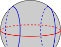
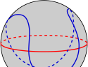
Figure 3. Identifying a pair of hemispheres, each endowed with $k$ disjoint arcs, by a common equator we sometimes get a meander and sometimes — not.

Consider now a collection of $k$ disjoint arcs on the northern hemisphere and a collection of the same number of disjoint arcs on the southern hemisphere. Assume that the endpoints of the arcs are equidistant on the equators. Denote by $n$ the total number of minimal arcs (the ones, for which the endpoints are neighbors on the equator) on two hemispheres. We computed in [DGZZ2] the asymptotic probability $\operatorname{P}_{0,n}$ that a random gluing of a random pair of arcs as above with $k\leq N$ gives a meander, see Figure 3. As in the other problems, the asymptotics is computed for a fixed $n$ letting $N\to+\infty$. In the current paper we derive general formulas for probabilities to get a meander under analogous identification of endpoints of compatible random collections of disjoint arcs on a surface of any genus $g$ with two boundary components. We consider this problem in various settings and under various asymptotic regimes.

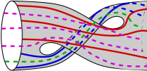
Figure 4. Collection of disjoint strands joining two boundary components of a surface of genus $1$

We also consider random collections of disjoint strands on a connected surface of genus $g-1$ with two boundary components. Assuming that each strand goes from one component to another, as in Figure 4, we compute asymptotic probability $\operatorname{P}^{+}_{g}$ that upon a random gluing of two boundary components matching the endpoints of strands one gets a single connected closed curve, or, in other words, an oriented meander. For genus $g=1$ the surface of genus $g-1$ with boundary is a cylinder and the problems reduces to computation of asymptotic probability that random positive integers $(k,m)$, such that $m\leq k$, are coprime. In this case the answer $\operatorname{P}^{+}_{1}=\frac{6}{\pi^{2}}$ is elementary. However, already for genus $g=2$ as in Figure 4 we do not know any way to compute $\operatorname{P}^{+}_{2}=\frac{45}{2\pi^{4}}$ other than applying technique involving the Masur–Veech volume $\operatorname{Vol}\mathcal{H}_{2}$ of the moduli spaces $\mathcal{H}_{2}$ of Abelian differentials. This technique allows us to produce a list of exact values of $\operatorname{P}^{+}_{g}$ up to $g=1000$ in several seconds. For large $g$ we prove the asymptotic formula $\operatorname{P}^{+}_{g}=\frac{1}{4g}\left(1+\frac{12+\pi^{2}}{24g}+O\left(\frac{1}{g^{2}}\right)\right)$.

One more open problem of Arnold, asking what is the probability that the decomposition of a random “interval exchange permutation” into disjoint cycles contains a single cycle, is closely related to evaluation of $\operatorname{P}^{+}_{g}$. This problem admits a solution by methods developed below, but we will treat it separately to avoid overloading the paper.

1.3. Technique of the proofs

We start with an idea from our work [DGZZ2] on meander count in genus $0$, namely, we translate the problem into the language of count of square-tiled surfaces closely related to evaluation of the Masur–Veech volumes of moduli spaces of meromorphic quadratic differentials. However, while in [DGZZ2] this translation, basically, completes the solution of the problem, in the current paper it serves as a starting point. Combinatorics of graphs on a sphere is in certain aspects much simpler than on higher genus surfaces. In particular, the count of single-band square-tiled surfaces is simple only in the case of genus $0$. Furthermore, by work of J. Athreya, A. Eskin and A. Zorich [AEZ2] the Masur–Veech volume of any stratum in genus $0$ is given by a simple closed formula, while in higher genera an efficient algorithm providing explicit volumes of general strata, different from the principal one, is not known yet beyond strata of dimension $12$. (Volumes of all low-dimensional strata of quadratic differentials were evaluated by E. Goujard [Gj] based on the general algorithm developed by A. Eskin and A. Okounkov [EO2].) By these reasons the results of the current paper were out of reach at the time when [DGZZ2] was written.

In order to study higher genus meanders, we apply recent technique of evaluation of Masur–Veech volumes of moduli spaces of Abelian and quadratic differentials. More concretely, we use most of spectacular advances in the study of Masur–Veech volumes obtained by A. Aggarwal in [Ag1], [Ag2], and by D. Chen, M. Möller, A. Sauvaget, D. Zagier in [CMSZ], [CMS], [Svg1], [Svg2]. We also use developments of these results by M. Kazarian [Kz] and by D. Yang, D. Zagier, Y. Zhang [YZZ]; see also a related work of J. Guo and of D. Yang [GY]. Finally, we also actively use our own recent results on Masur–Veech volumes of the principal strata of quadratic differentials [DGZZ3], [DGZZ4] and the count of square-tiled surfaces [DGZZ1], developed, in particular, in view of applications to meanders count. One of the main technical tools of the current paper consists in the count of square-tiled surfaces through Witten–Kontsevich correlators (intersection numbers of $\psi$-classes) obtained in [DGZZ3]. In the context of meanders we need only $1$- and $2$-correlators. The $1$-correlators admit a closed formula [Wi], and the $2$-correlators admit a linear recursion [Zog1] and precise estimates [DGZZ3].

While for general genus $g$ meanders we obtain only a restricted count corresponding to a fixed number $n$ of bigons, for oriented meanders we solve the enumeration problem completely. We also obtain a precise large genus asymptotic count of oriented meanders.

Remark 1.3.

Count of square-tiled surfaces through Witten–Kontsevich correlators, performed in our paper [DGZZ3], is closely related to the count of asymptotic frequencies of simple closed geodesics on a hyperbolic surface performed by M. Mirzakhani [Mi2]. As a byproduct of the count of genus $g$ meanders, we compare in the current paper the frequencies of separating versus non separating simple closed geodesics on surfaces of a large genus $g$ with $n$ cusps. Numerous quantities responsible for geometry of a hyperbolic surface of a large genus $g$ with $n$ cusps are very sensitive to the growth rate of the number of cusps compared to the growth rate of the genus, see results [Ag2] of A. Aggarwal on Witten–Kontsevich correlators or results by W. Hide [Hi], W. Hide and M. Magee [HiM], W. Hide and J. Thomas [HiT], of N. Anantharaman and L. Monk [AnMo], T. Budzinski, N. Curien, B. Petri [BCP], M. Lipnowski and A. Wright [LiWr], Yunhui Wu and Yuhao Xue [WuXue], Yang Shen and Yunhui Wu [ShWu], and of P. Zograf [Zog2] on the spectral gap and on the Cheeger constant of hyperbolic surfaces of large genus with cusps. We show in this paper that the frequencies of separating versus non separating simple closed geodesics have very limited dependence on number of cusps in large genus.

1.4. Structure of the paper

Section 2 provides accurate definitions of higher genus meanders and arc systems, and presents the main counting results. All the results follow from the correspondence between meanders and square-tiled surfaces. The latter represent integer points in moduli spaces of quadratic or Abelian differentials. Section 3 recalls necessary facts on the count of square-tiled surfaces; Section 4 describes the above mentioned correspondence.

Having established this count we complete the proofs of those results stated in Section 2 which concern fixed genus $g$ and fixed number of bigons $n$.

Section 6 is devoted to analysis of the resulting count in two complementary asymptotic regimes: when the number $n$ of bigons is fixed and the genus $g$ grows and when the genus is fixed and the number $n$ of bigons grows. Here we transpose recent advances in asymptotics of the Masur–Veech volumes of moduli spaces of Abelian and quadratic differentials mentioned above to asymptotic count of meanders. As an application we compute the asymptotic probability that a random simple closed geodesic on a hyperbolic surface of genus $g$ with $n$ cusps is separating in the regime when the number of cusps $n$ is fixed and the genus $g$ tends to infinity and in the regime when the genus $g$ is fixed while the number of cusps $n$ tends to infinity stated in Section 2.3.

We complete the paper with two Appendices. Consider the graph $\mathcal{G}$ formed by a meander on a surface of genus $g$. For a fixed number $n$ of bigons, the total number of boundary components of $S-\mathcal{G}$ formed by $6$ and more edges is bounded above by $4g-4+n$ independently of the number $2N$ of intersections of a meander. All the remaining boundary components are bounded by exactly $4$ edges. In appendix A we perform a restricted count of the asymptotic number of meanders with at most $2N$ intersections on a surface of genus $g$ imposing to a meander not only a fixed number $n$ of bigons in $S-\mathcal{G}$, but also fixing the numbers of $6$-gons, $8$-gons, etc.

Appendix B might represent an independent interest with no relation to meanders. Namely, we compute asymptotics of the sum of the form $\sum_{k}\cfrac{\binom{a_{1}n+b_{1}}{c_{1}k+d_{1}}\cdots\binom{a_{l}n+b_{l}}{c_{l}k+d_{l}}}{\binom{s_{1}n+t_{1}}{u_{1}k+v_{1}}\cdots\binom{s_{m}n+t_{m}}{u_{1}k+v_{m}}}$ under assumptions that $\frac{a_{1}}{c_{1}}=\dots=\frac{a_{l}}{c_{1}}=\frac{s_{1}}{u_{1}}=\dots=\frac{s_{m}}{u_{m}}$ and that $a_{1}+\dots+a_{l}>s_{1}+\dots+s_{m}$. Particular cases of this computation are used in Section 6. Another particular case allows us to derive large genus asymptotics of the sums $\sum_{k=0}^{3g-1}\langle\tau_{k}\tau_{3g-1-k}\rangle_{g}$ of Witten–Kontsevich 2-correlators used in Section 6.

Acknowledgments. We are grateful to A. Aggarwal, C. McMullen, F. Petrov, A. Zvonkin for helpful questions and comments. We thank L. Monk and to B. Petri for clarifying to us dependence of properties of hyperbolic surfaces in different regimes when either genus or the number of cusps are growing, see Remark 1.3. We thank I. Ren for indicating us several typos in the manuscript.

2. Transverse multicurves, meanders and arc systems

2.1. Count of higher genus meanders

In this paper we consider only simple curves on oriented smooth surfaces, where simple means that the curve is smoothly embedded into the surface, i.e. does not have self-intersections, self-tangencies or cusps. In this paper we do not exclude closed curves homotopic to a point. We reserve the notions arc and strand for topological segments. In all our considerations closed curves live on closed surfaces, while non-closed curves (i.e. arcs and strands) live on surfaces with boundaries, have endpoints at boundary components and are transverse to the boundaries. By convention, endpoints of an arc might belong to the same or to different boundary components, while the endpoints of a strand necessarily belong to distinct boundary components. A multicurve is a finite collection of pairwise disjoint simple closed curves. In particular, in this paper we do not use integral weights to encode freely homotopic connected components of a multicurve.

Definition 2.1.

We say that an ordered pair of multicurves forms a connected transverse pair if both of the following conditions are satisfied: all pairs of components of multicurves intersect transversally and the graph $\mathcal{G}$ obtained as a union of two multicurves is connected. The pair is filling if it cuts the surface into topological disks, or, equivalently, if the graph $\mathcal{G}$ is a map.

By convention, the first multicurve in a connected transverse pair of multicurves is called horizontal and the second one — vertical. We consider natural equivalence classes of pairs of transverse multicurves up to diffeomorphisms preserving orientation of the surface and the horizontal and vertical multicurves.

Remark 2.2.

Note that speaking of a “multicurve” one usually assumes that the components of a multicurve are neither contractible nor peripheral (i.e. not freely homotopic to a boundary component). Given a connected filling transverse pair of multicurves in the sense of Definition 2.1 make a single puncture at every bigon. We will see in Section 4 that each component of the horizontal (respectively vertical) multicurve on the resulting punctured surface is neither contractible nor peripheral, so we get a multicurve in the usual sense.

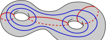
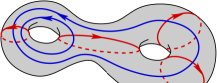
Figure 5. Both connected pairs of transverse multicurves are filling, but the pair on the left is nonorientable, while the pair on the right is oriented.

Definition 2.3.

A transverse pair of multicurves is called positively oriented (or just oriented for brevity) if each connected component of each multicurve is oriented in such way that any individual intersection of any connected component of the horizontal multicurve with any connected component of the vertical multicurve matches the orientation of the surface. In other words, the intersection number of any connected component of the horizontal multicurve with any connected component of the vertical multicurve coincides with the naive number of intersections. A transverse pair of multicurves is called orientable if it admits the above structure and nonorientable otherwise, see Figure 5 for an illustration.

Definition 2.4.

A meander of genus $g$ is a connected pair of transverse simple closed curves on a surface of genus $g$. Similarly, an orientable meander of genus $g$ is an orientable connected pair of transverse simple closed curves on a surface of genus $g$ (see Figure 5 for an illustration). Fixing an orientation of an orientable meander, we get an orientable meander. Meanders of genus $g>0$ are called higher genus meanders.

An orientable meander admits two distinct orientations unless there exists a diffeomorphism of the surface sending the meander to itself and reversing the orientation of each of the two simple closed curves. There are no orientable meanders in genus 0.

Following the notation for count of classical meanders on a sphere (which fits traditional conventions on count of square-tiled surfaces in strata of meromorphic quadratic differentials) we denote by $\operatorname{M}_{g,n}(N)$ the number of genus $g$ meanders with at most $2N$ crossings and exactly $n$ bigons, see Definition (1.1). It would be convenient to denote by $\operatorname{M}_{g}^{+}(N)$ the number of orientable genus $g$ meanders with at most $N$ (and not $2N$) crossings, see Figure (6) for an illustration.

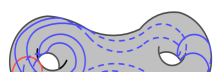
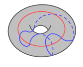
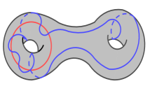
Figure 6. Meander on the left contributes to $\operatorname{M}^{+}_{2}(4)$; in the middle — to $\operatorname{M}_{1,2}(2)$; on the right — to $\operatorname{M}_{2,4}(3)$.

Theorem 2.5.

For any nonnegative numbers $g$ and $n$ satisfying $2g+n\geq 4$, the number $\operatorname{M}_{g,n}(N)$ of meanders with exactly $n$ bigons on a surface of genus $g$ and with at most $2N$ crossings satisfies the following asymptotics:

(2.1) $$\operatorname{M}_{g,n}(N)=C_{g,n}N^{6g-6+2n}+o(N^{6g-6+2n})\quad\text{as }N\to\infty\,,$$

with

(2.2) $$C_{g,n}=\frac{cyl_{1,1}({\mathcal{Q}}_{g,n})}{(4g-4+n)!\,n!\,(12g-12+4n)}\,.$$

Here

(2.3) $$cyl_{1,1}({\mathcal{Q}}_{g,n})=\frac{\big{(}cyl_{1}({\mathcal{Q}}_{g,n})\big{)}^{2}}{\operatorname{Vol}{\mathcal{Q}}_{g,n}}$$

is a rational multiple of $\pi^{-6g+6-2n}$, where $\operatorname{Vol}{\mathcal{Q}}_{g,n}$ denotes the Masur–Veech volume of the moduli space of quadratic differentials, and $cyl_{1}({\mathcal{Q}}_{g,n})$ denotes the contribution of single-band square-tiled surfaces to this volume. The quantities $\operatorname{Vol}{\mathcal{Q}}_{g,n}$ and $cyl_{1}({\mathcal{Q}}_{g,n})$ are expressed in terms of intersection numbers of $\psi$-classes by formulas (6.6) and (6.20)–(6.24) respectively.

All but negligible (as $N\to+\infty$) part of meanders as above are nonorientable, filling, and have only bigonal, quadrangular and hexagonal faces.

For any fixed value of $g$ we have

(2.4) $$C_{g,n}\sim\frac{1}{8\pi^{2}}\cdot\frac{a_{g}^{2}}{\kappa_{g}}\cdot\frac{1}{n^{\frac{5}{2}g-1}}\cdot\left(\frac{32\cdot e^{2}}{\pi^{2}\cdot n^{2}}\right)^{n}\ \text{as }n\to\infty\,;$$

where $a_{g}$ and $\kappa_{g}$ are given by Equations (6.28) and (6.35) respectively.

For any fixed value of $n$ we have:

(2.5) $$C_{g,n}\sim\frac{1}{32}\sqrt{\frac{3}{2\pi}}\cdot\frac{1}{n!}\cdot\left(\frac{4}{3g}\right)^{n-\frac{3}{2}}\cdot\left(\frac{2e}{3g}\right)^{4g}\ \text{as }g\to\infty\,.$$

The polynomial asymptotics (2.1) and the fact that the coefficient of the leading term is given by expression (2.2) is proved in Section 5. Asymptotic relation (2.4) is proved at the end of Section 6.3. Asymptotic relation (2.5) is proved at the end of Section 6.4.

This result can be compared to the following natural exponential bounds for the number of meanders on surfaces of genus $g$, with no constraints on the number of bigons:

Lemma 2.6.

The number $M_{g}^{=N}$ of meanders with exactly $2N$ crossings on a surface of genus $g$ satisfies the following bounds:

$$C_{N}\leq M_{0}^{=N}\leq M_{g}^{=N}\leq 2N\cdot p_{g}(2N+1)\cdot C_{2N+1}\left(1+o(1)\right)\ \text{ as }N\to+\infty\,,$$

where $C_{N}=\frac{1}{N+1}\binom{2N}{N}$ is the $N$-th Catalan number, and $p_{g}$ is an explicit polynomial of degree $3g$.

Lemma 2.6 is proven in Section 5.

Theorem 2.7.

For any genus $g\geq 1$, the number $\operatorname{M}_{g}^{+}(N)$ of oriented meanders with at most $N$ crossings satisfies the following asymptotics:

(2.6) $$\operatorname{M}_{g}^{+}(N)=C_{g}^{+}N^{4g-3}+o(N^{4g-3})\quad\text{as }N\to\infty\,,$$

where

(2.7) $$C_{g}^{+}=\frac{cyl_{1,1}(\mathcal{H}_{g})}{(2g-2)!(8g-6)}\,.$$

Here $cyl_{1,1}(\mathcal{H}_{g})=\frac{\left(cyl_{1}(\mathcal{H}_{g})\right)^{2}}{\operatorname{Vol}\mathcal{H}_{g}}$ is a rational multiple of $\frac{1}{\pi^{2g}}$, where $\operatorname{Vol}\mathcal{H}_{g}$ denotes the Masur–Veech volume of the moduli space of Abelian differentials $\mathcal{H}_{g}$ and

$$cyl_{1}(\mathcal{H}_{g})=\frac{1}{2^{2g-4}(4g-2)}$$

is the contribution of single-band square-tiled surfaces to this volume.

Moreover, $C_{g}^{+}$ satisfies the following asymptotics

(2.8) $$\frac{1}{4\sqrt{\pi}}\cdot\frac{1}{g^{\frac{3}{2}}}\left(\frac{e}{4g}\right)^{2g}\left(1+\frac{29+\pi^{2}}{24g}+O\left(\frac{1}{g^{2}}\right)\right)\quad\text{as }g\to\infty\,.$$

The polynomial asymptotics (2.6) and the fact that the coefficient of the leading term is given by expression (2.7) is proved in Section 5. Asymptotic relation (2.8) is proved in Corollary 6.10 in Section 6.5.

Using the correspondence between meanders and flat surfaces we perform a more detailed count for higher genus meanders fixing not only the number $n$ of bigons but also the number of $6$-gons, $8$-gons etc. This detailed count is presented in Appendix A. However, in the most general non-orientable case, at the current stage of knowledge of Masur–Veech volumes of general strata of quadratic differentials, one can transform our formulas into actual rational numbers only for small values of $g$ and $n$.

Meandric systems. Traditionally, one represents a multicurve as a weighted sum $\gamma=h_{1}\gamma_{1}+\dots+h_{m}\gamma_{m}$ of the primitive components $\gamma_{1},\dots,\gamma_{m}$, which are already not pairwise freely homotopic on the punctured surface (see Remark 2.2), and where the positive integer weight $h_{i}$ encodes the number of components of the multicurve $\gamma$ freely homotopic to the primitive component $\gamma_{i}$ for $i=1,\dots,m$.

The number of components of a multicurve $\gamma=h_{1}\gamma_{1}+\dots+h_{m}\gamma_{m}$ is given by the sum $h=h_{1}+\dots+h_{m}$ of the weights, where $m$ is the number of primitive components.

One can define meandric systems by allowing the vertical multicurve to have several components. Meandric systems were recently studied in [CuKST], [FeT] [FuNe], [GnNP], [Kg] (see these papers for further references). The results of [DGZZ4] provide the large genus asymptotic distribution of the number $m$ of primitive components of those meandric systems, which do not have any bigons. The genus zero case with a fixed number of bigons was studied in slightly different terms in [AEZ1].

The question of the distribution of the actual number $h$ of components in large genus is still open, some conjectures about this distribution will be presented in a subsequent paper.

2.2. Asymptotic probability of getting a meander from an arc system

Consider a transverse pair of multicurves such that the horizontal multicurve is just a single simple closed curve. Cutting the surface by this horizontal curve we get an arc system as in Figure 7. The cut surface has one or two connected components depending on whether the simple closed curve is separating or not.

Definition 2.8.

A balanced arc system of genus $g$ is a finite collection of smooth pairwise nonintersecting segments (called arcs) on a smooth oriented surface with two boundary components (a single connected surface of genus $g-1$ with two boundary components or two connected surfaces of genera $g_{1},g_{2}$ satisfying $g_{1}+g_{2}=g$, each with a single boundary component), satisfying all of the following conditions:

• the endpoints of all segments are located at the boundary;

• each segment approaches the boundary transversally;

• the numbers of endpoints of the segments on one boundary components is the same as on the other boundary component (and, hence, equals the number of arcs).

The arc system is filling if the segments cut the surface into a collection of topological disks.

Throughout this paper we consider only balanced arc systems, even when it is not stated explicitly.

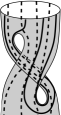
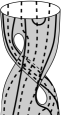
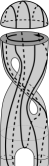
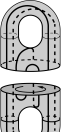
Figure 7. A random identification of a random balanced arc system with large number of arcs gives a meander with one and the same asymptotic probability exceeding $1/4$ for each of the four types of arc systems as in the picture, see Example 2.11.

Identifying the boundary components of a surface endowed with a balanced arc system by a diffeomorphism which matches the endpoints of the arcs and arranges them into smooth curves we get a transverse pair of multicurves where the horizontal one is connected. We use only those identifications of the boundary which lead to an oriented surface. The following question seems to us natural to address: what is the probability to obtain a meander by this construction? We have an answer to this question, on average in the following sense.

Up to a Dehn twist along the boundary component, there are (at most) $k$ distinct identifications of the two boundary components of a surface endowed with a balanced arc system containing $k$ arcs, matching the endpoints of the arcs. (The number of distinct identifications is less than $k$ when the arc system admits symmetries.)

Fix the genus $g$ and the number $n$ of bigons. We always assume that $2g+n\geq 4$. Fix the upper bound $N$ for the number of arcs. Denote by $\operatorname{AS}_{g,n}(N)$ the number of all possible couples (balanced arc system of genus $g$ with $n$ bigons with $k\leq N$ arcs; identification) considered up to a natural equivalence. Denote by $\operatorname{MAS}_{g,n}(N)$ the number of those couples, which give rise to a meander. Define

$$\operatorname{P}_{g,n}(N)=\frac{\operatorname{MAS}_{g,n}(N)}{\operatorname{AS}_{g,n}(N)}\,.$$

Recall that by convention $g$ denotes the genus of the surface obtained after identification of the two boundary components.

Theorem 2.9.

The proportion of balanced arc systems of genus $g$ with $n$ bigons giving rise to meanders among all such arc systems has a limiting value

(2.9) $$\lim_{N\to\infty}\operatorname{P}_{g,n}(N)=\operatorname{P}_{\!g,n}\,,$$

which coincides with the relative contribution $p_{1}({\mathcal{Q}}_{g,n})$ of single-band square-tiled surfaces to the Masur–Veech volume $\operatorname{Vol}{\mathcal{Q}}_{g,n}$. The quantity

(2.10) $$\operatorname{P}_{\!g,n}=p_{1}({\mathcal{Q}}_{g,n})=\frac{cyl_{1}({\mathcal{Q}}_{g,n})}{\operatorname{Vol}{\mathcal{Q}}_{g,n}}$$

is a rational multiple of $\pi^{-6g+6-2n}$, where $\operatorname{Vol}{\mathcal{Q}}_{g,n}$ denotes the Masur–Veech volume of the moduli space of quadratic differentials, and $cyl_{1}({\mathcal{Q}}_{g,n})$ denotes the contribution of single-band square-tiled surfaces to this volume. The quantities $\operatorname{Vol}{\mathcal{Q}}_{g,n}$ and $cyl_{1}({\mathcal{Q}}_{g,n})$ are expressed in terms of intersection numbers of $\psi$-classes by Formulas (6.6) and (6.20)–(6.24) respectively.

Moreover, for any fixed value of $g$ we have

(2.11) $$p_{1}({\mathcal{Q}}_{g,n})\sim\frac{1}{\sqrt{\pi}}\cdot\frac{a_{g}}{\kappa_{g}}\cdot n^{\frac{g-1}{2}}\left(\frac{8}{\pi^{2}}\right)^{n}\quad\text{as }n\to\infty\,,$$

where $a_{g}$ and $\kappa_{g}$ are given by Equations (6.28) and (6.35) respectively.

For any fixed $n$:

(2.12) $$p_{1}({\mathcal{Q}}_{g,n})\sim\frac{\sqrt{6\pi}}{12}\cdot\frac{1}{\sqrt{g}}\,,\quad\text{as }g\to\infty\,.$$

The existence of the limit $\lim_{N\to\infty}\operatorname{P}_{\!g,n}(N)$ and expression (2.10) for its value are proved at the end of Section 5. Asymptotic relations (2.11) and (2.12) are proved in Corollaries 6.7 and 6.9 respectively.

Formulas (6.6) and (6.20)–(6.24) for $\operatorname{Vol}{\mathcal{Q}}_{g,n}$ and $cyl_{1}({\mathcal{Q}}_{g,n})$ lead to closed expressions for any fixed genus $g$ as a function of $n$. For example,

$$p_{1}({\mathcal{Q}}_{0,n}) =\frac{1}{2}\left(\frac{2}{\pi^{2}}\right)^{n-3}\binom{2n-4}{n-2}\,,$$

$$p_{1}({\mathcal{Q}}_{1,n}) =\cfrac{2}{\pi^{2n}}\cdot\cfrac{4\cdot\binom{2n-2}{n-1}+\frac{1}{48}\cdot\binom{2n-1}{n-2}-\frac{n^{2}-n+2}{96}}{\frac{n!}{(2n-1)!!}+\frac{2n}{(2n-1)2^{n}}}\,.$$

We can choose a setting, in which we consider subsets of arc systems as above sharing a more restricted topology. Namely, when $g$ is strictly positive, we can separately consider arc systems on a surface of genus $g-1$ with two boundary components, as on the left two pictures in Figure 7. We can also fix a partition of $n$ minimal arcs into $n_{1}\geq 0$ arcs adjacent to the first boundary component and $n_{2}\geq 0$ arcs adjacent to the second boundary component, where $n_{1}+n_{2}=n$. If $g=1$, we assume that $n\geq 2$ and that $n_{i}\geq 1$ for $i=1,2$. Fixing $g,n_{1},n_{2}$ as above and the bound $N$ for the number of arcs, denote by $\operatorname{AS}_{g,n_{1},n_{2}}(N)$ the number of all possible couples (balanced arc system with $n_{i}$ bigons at the $i$-th boundary component, where $i=1,2$, with at most $k\leq N$ arcs on a connected surface of genus $g-1$ with two boundary components; identification) considered up to a natural equivalence. Denote by $\operatorname{MAS}_{g,n_{1},n_{2}}(N)$ the number of those couples, which give rise to a meander. Define

$$\operatorname{P}_{g,n_{1},n_{2}}(N)=\frac{\operatorname{MAS}_{g,n_{1},n_{2}}(N)}{\operatorname{AS}_{g,n_{1},n_{2}}(N)}\,.$$

Alternatively, we can chose any nonnegative integers $g_{1},g_{2}$ such that $g_{1}+g_{2}=g$ and consider two connected surfaces of genera $g_{1}$ and $g_{2}$ respectively, each having a single boundary component, as on the right two pictures in Figure 7. We can also consider any partition $n_{1}+n_{2}=n$ of $n$ into an ordered sum of nonnegative integers satisfying the following condition: if $g_{i}=0$, for any of $i=1,2$, then $n_{i}\geq 2$. Denote by $\operatorname{AS}_{g,n_{1}}^{g_{2},n_{2}}(N)$ the number of all possible couples (balanced arc system on a surface having two connected components of genera $g_{1}$ and $g_{2}$, each with a single boundary component, with $n_{1}$ bigons on the first component, with $n_{2}$ bigons on the second component and with $k\leq N$ arcs; identification). considered up to a natural equivalence. Denote by $\operatorname{MAS}_{g,n_{1}}^{g_{2},n_{2}}(N)$ the number of those couples, which give rise to a meander. Define

$$\operatorname{P}^{g_{2},n_{2}}_{g_{1},n_{1}}(N)=\frac{\operatorname{MAS}_{g,n_{1}}^{g_{2},n_{2}}(N)}{\operatorname{AS}_{g,n_{1}}^{g_{2},n_{2}}(N)}\,.$$

Theorem 2.10.

For any $g,n,g_{1},g_{2},n_{1},n_{2}$ satisfying the above requirements one has

(2.13) $$\lim_{N\to\infty}\operatorname{P}_{g,n_{1},n_{2}}(N)=\lim_{N\to\infty}\operatorname{P}^{g_{2},n_{2}}_{g_{1},n_{1}}(N)=\operatorname{P}_{\!g,n}\,,$$

Theorem 2.10 is proved at the end of Section 5.

Example 2.11.

Consider a random balanced arc system of any of the four types schematically presented in Figure 7. One should, actually, take much more arcs than in the picture, maintaining, however, a location of the only two minimal arcs in each of the four cases. Theorem 2.10 affirms, in particular, that a random identification of boundary components of such an arc system we obtain a meander with asymptotic probability

$$\lim_{N\to\infty}\operatorname{P}_{2,2,0}(N)=\lim_{N\to\infty}\operatorname{P}_{2,1,1}(N)=\lim_{N\to\infty}\operatorname{P}^{1,1}_{1,1}(N)=\lim_{N\to\infty}\operatorname{P}^{2,0}_{0,2}(N)\operatorname{P}_{2,2}=\frac{9\,230\,760}{337\cdot\pi^{10}}\approx 0.292489$$

for each of the four types of arc systems as in Figure 7. The numerical value of $\operatorname{P}_{2,2}$ given by Formula (2.10), uses the value $\operatorname{Vol}{\mathcal{Q}}_{2,2}=\frac{337}{18144}\pi^{10}$ evaluated by means of Formula (6.6) and the value $cyl_{1}({\mathcal{Q}}_{2,2})=\frac{2035}{4}$ evaluated by means of Formula (6.24).

Oriented arc systems (collections of strands). Consider a closed oriented surface endowed with a connected transverse pair of multicurves, such that the horizontal multicurve is a single simple closed curve. Cutting the surface by the horizontal curve we get an oriented arc system, or equivalently, a collection of disjoint strands, each strands joining one boundary component to another, as in Figure 4. Reciprocally, having a connected oriented surface with two boundary components, and a system of disjoint strands joining the boundary components and approaching them transversally, we can identify boundary components in a way which matches the endpoints of the strands, and get a connected transverse pair of multicurves, where the horizontal multicurve is a single simple closed curve. By construction, the resulting transverse pair of multicurves is always orientable. Choosing the orientation of the horizontal curve or of any strand, we uniquely determine the orientation of the resulting pair of multicurves. As before, when there are $k$ strands, there are (at most) $k$ distinct identifications of the two boundary components, matching the endpoints of the arcs, up to a Dehn twist along the boundary component. The number of distinct identification is less than $k$ when the arc system admits symmetries.

Fix the genus $g-1$ of the connected oriented surface with two boundary components and the upper bound $N$ for the number of strands. Denote by $\operatorname{AS}_{g}^{+}(N)$ the number of all possible couples (oriented arc system with at most $N$ strands on a surface of genus $g-1$; identification) and by $\operatorname{MAS}_{g}^{+}(N)$ the number of couples as above which give ride to a meander. Define

$$\operatorname{P}_{\!g}^{+}(N)=\frac{\operatorname{MAS}_{g}^{+}(N)}{\operatorname{AS}_{g}^{+}(N)}\,.$$

Theorem 2.12.

The proportion of oriented arc systems of genus $g$ giving rise to oriented meanders among all such arc systems satisfies

(2.14) $$\lim_{N\to\infty}\operatorname{P}_{\!g}^{+}(N)=\operatorname{P}_{\!g}^{+}\,.$$

Here

(2.15) $$\operatorname{P}_{\!g}^{+}=p_{1}(\mathcal{H}_{g})=\frac{cyl_{1}(\mathcal{H}_{g})}{\operatorname{Vol}\mathcal{H}_{g}}$$

is a rational multiple of $\pi^{-2g}$, where $\operatorname{Vol}\mathcal{H}_{g}$ denotes the Masur–Veech volume of the moduli space of Abelian differentials, and $cyl_{1}(\mathcal{H}_{g})=\frac{1}{(2g-1)\cdot 2^{2g-3}}$ denotes the contribution of single-band square-tiled surfaces to this volume.

Moreover,

(2.16) $$p_{1}(\mathcal{H}_{g})=\frac{1}{4g}\left(1+\frac{12+\pi^{2}}{24g}+O\left(\frac{1}{g^{2}}\right)\right)\quad\text{as }g\to+\infty\,.$$

The existence of the limit $\lim_{N\to\infty}\operatorname{P}_{\!g}^{+}(N)$ and expression (2.15) for its value are proved at the end of Section 5. Asymptotic relation (2.16) is proved in Corollary 6.10 in Section 6.5.

2.3. Count of simple closed geodesics on hyperbolic surfaces with cusps

We pass now to a different problem concerning closed geodesics on hyperbolic surfaces, that we are able to solve using the techniques developed in this paper. We refer to [DGZZ3] for more details about the relation between this problem and the evaluation of Masur–Veech volumes.

M. Mirzakhani has counted in [Mi2] asymptotic frequencies of simple closed geodesics (and, more generally, of simple closed geodesic multi-curves) on a hyperbolic surface of genus $g$ with $n$ cusps. We distinguish the non-separating simple closed geodesics and the separating ones. In the latter case we count all separating simple closed geodesics, no matter the resulting decomposition of the surface of genus $g$ with $n$ cusps into two subsurfaces of genera $g_{1}+g_{2}=g$ and no matter how the cusps are partitioned between the two subsurfaces. Denote by $c_{g,n,\mathrm{sep}}$ and by $c_{g,n,\mathrm{nonsep}}$ the corresponding Mirzakhani’s frequencies.

Our asymptotic count of meanders in the regime when one of the two parameters $g,n$ is fixed and the other tends to infinity implies the following two results (namely, Theorems 2.13 and 2.15) on asymptotic count of simple closed hyperbolic geodesics.

Theorem 2.13.

The ratio of frequencies of separating over nonseparating simple closed geodesics on a closed hyperbolic surface of genus $g=1$ with $n$ cusps has the following asymptotics:

(2.17) $$\lim_{n\to\infty}\frac{c_{1,n,\mathrm{sep}}}{c_{1,n,\mathrm{nonsep}}}=\frac{1}{6}\,.$$

The ratio of frequencies of separating over nonseparating simple closed geodesics on a closed hyperbolic surface of genus $g\geq 2$ with $n$ cusps has the following asymptotics:

(2.18) $$\lim_{n\to\infty}\frac{c_{g,n,\mathrm{sep}}}{c_{g,n,\mathrm{nonsep}}}=\frac{1}{12^{g}\cdot g!\cdot\sum_{k=0}^{3g-4}\langle\tau_{k}\tau_{3g-4-k}\rangle_{g-1}}\,,$$

where $\langle\tau_{k}\tau_{3g-4-k}\rangle_{g-1}$ are the Witten–Kontsevich correlators which can be computed recursively by formulas (6.12)–(6.14).

Remark 2.14.

M. Mirzakhani proved that the ratio $\frac{c_{g,n,\mathrm{sep}}}{c_{g,n,\mathrm{nonsep}}}$ is shared by all hyperbolic surfaces of genus $g$ with $n$ cusps, see [Mi2, Corollary 1.4]. In particular, taking a very symmetric hairy torus, which has marked points at $n^{2}$ torsion points of your favorite elliptic curve as in the example from [Br, Section 5.3] or any other randomly chosen hairy torus with a very large number of cusps a random simple closed geodesics happens to be separating with the same asymptotic probability $\frac{1}{7}$.

$$\begin{array}[]{|c|c|c|c|c|c|c|c|c|c|}\hline\cr g&1&2&3&4&5&6&7&8&9\\ \hline\cr&&&&&&&&&\\[-6.0pt] &\frac{1}{6}&\frac{1}{36}&\frac{5}{882}&\frac{35}{28344}&\frac{7}{25218}&\frac{77}{1210716}&\frac{143}{9686190}&\frac{715}{206641008}&\frac{12155}{14878191186}\\[-6.0pt] &&&&&&&&&\\ \hline\cr\end{array}$$

Table 1. Values of $\lim_{n\to\infty}\frac{c_{g,n,\mathrm{sep}}}{c_{g,n,\mathrm{nonsep}}}$ for $g=1,\dots,9$.

Note that though for any fixed $g$ we get a nonzero limit, the right-hand side of (2.18) rapidly decreases when $g$ grows. Table 1 provides the exact values of the expression in the right-hand side of (2.18) for small genera $g$.

The asymptotic value of the sum of $2$-correlators in genus $g$ computed in (B.14) in Appendix B.3 implies the following asymptotics for the expression in the right-hand side of (2.18):

(2.19) $$\frac{1}{12^{g}\cdot g!\cdot\sum_{k=0}^{3g-4}\langle\tau_{k}\tau_{3g-4-k}\rangle_{g-1}}\sim\frac{2}{\sqrt{3\pi g}}\cdot\frac{1}{4^{g}}\quad\text{as }g\to+\infty\,.$$

Theorem below describes the asymptotics of the ratio $\frac{c_{g,n,\mathrm{sep}}}{c_{g,n,\mathrm{nonsep}}}$ in the complementary regime, when the number $n$ of cusps is fixed and $g\to+\infty$.

Theorem 2.15.

For any fixed number $n\geq 0$ of cusps, the ratio of frequencies of separating over nonseparating simple closed geodesics on a closed hyperbolic surface of genus $g$ has the following asymptotics:

(2.20) $$\frac{c_{g,n,\mathrm{sep}}}{c_{g,n,\mathrm{nonsep}}}\sim\sqrt{\frac{2}{3\pi g}}\cdot\frac{1}{4^{g}}\quad\text{as }g\to+\infty\,.$$

In particular, it does not depend on $n$, as soon as $n$ is fixed.

Theorem 2.15 is proved in Section 6.4.

Morally, the asymptotics (2.19) represents the ratio $\frac{c_{g,n,\mathrm{sep}}}{c_{g,n,\mathrm{nonsep}}}$ in the regime $1\ll g\ll n$, while the asymptotics (2.20) represents the ratio $\frac{c_{g,n,\mathrm{sep}}}{c_{g,n,\mathrm{nonsep}}}$ in the regime $1\ll n\ll g$. The resulting asymptotics differ by a factor $\sqrt{2}$. Numerical simulations suggest the following conjectural uniform asymptotics:

Conjecture 2.16.

​​​ The ratio of frequencies of separating over nonseparating simple closed geodesics on a closed hyperbolic surface of genus $g$ with $n$ cusps admits the following uniform asymptotics:

(2.21) $$\frac{c_{g,n,\mathrm{sep}}}{c_{g,n,\mathrm{nonsep}}}=\sqrt{\frac{2}{3\pi g}}\cdot\frac{1}{4^{g}}\cdot f\left(\frac{n}{g}\right)\big{(}1+\varepsilon(g,n)\big{)}\,,$$

where the function $f:[0;+\infty]\to\mathbb{R}$ is continuous and increases monotonously from $f(0)=1$ to $f(\infty)=\sqrt{2}$ and the error term $\varepsilon(g,n)$ tends to $0$ as $g\to+\infty$ uniformly in $n$.

Remark 2.17.

The above conjecture claims that the dependence of $\frac{c_{g,n,\mathrm{sep}}}{c_{g,n,\mathrm{nonsep}}}$ on the ratio $\frac{n}{g}$ is moderate for any hyperbolic surface of large genus. Such a behavior of asymptotic frequencies of simple closed geodesics is yet another manifestation of its topological nature in a contrast with geometric quantities, for which the regimes $n^{2}\ll g$ and $n^{2}\gg g$ are drastically different. For example, by the results of A. Aggarwal [Ag2, Theorem 1.5 and Remark 1.6], the normalized Witten–Kontsevich correlators are uniformly close to $1$ in the regime $n^{2}\ll g$ and might explode exponentially in the complementary regime. Similarly, by the results of Yang Shen and Yunhui Wu [ShWu] the spectral gap vanishes for Weil–Petersson random hyperbolic surfaces in the regime $n^{2}\gg g$ (at least under an extra technical assumption). See results cited in Remark 1.3 for more details.

3. Square-tiled surfaces and Masur–Veech volumes

In the current Section we recall the relevant information on the count of square-tiled surfaces. In the next Section 4 we express the count of higher genus meanders in terms of the count of certain special square-tiled surfaces and derive those results announced Section 2, which concern any fixed $g$ and $n$ from the results of the current Section.

3.1. Masur–Veech volume of the moduli space of quadratic differentials

Consider the moduli space $\mathcal{M}_{g,n}$ of complex curves of genus $g$ with $n$ distinct labeled marked points. The total space ${\mathcal{Q}}_{g,n}$ of the cotangent bundle over $\mathcal{M}_{g,n}$ can be identified with the moduli space of pairs $(C,q)$, where $C\in\mathcal{M}_{g,n}$ is a smooth complex curve with $n$ (labeled) marked points and $q$ is a meromorphic quadratic differential on $C$ with at most simple poles at the marked points and no other poles. In the case $n=0$ the quadratic differential $q$ is holomorphic. Thus, the moduli space of quadratic differentials ${\mathcal{Q}}_{g,n}$ is endowed with the canonical real symplectic structure. The induced volume element $d\!\operatorname{Vol}$ on ${\mathcal{Q}}_{g,n}$ is called the Masur–Veech volume element.

A non-zero quadratic differential $q$ in ${\mathcal{Q}}_{g,n}$ defines a flat metric $|q|$ on the complex curve $C$. The resulting metric has conical singularities at zeroes and simple poles of $q$. The total area of $(C,q)$

$$\operatorname{Area}(C,q)=\int_{C}|q|$$

is positive and finite. For any real $a>0$, consider the following subset in ${\mathcal{Q}}_{g,n}$:

$${\mathcal{Q}}^{\operatorname{Area}\leq a}_{g,n}:=\left\{(C,q)\in{\mathcal{Q}}_{g,n}\,|\,\operatorname{Area}(C,q)\leq a\right\}\,.$$

Since $\operatorname{Area}(C,q)$ is a norm in each fiber of the bundle ${\mathcal{Q}}_{g,n}\to\mathcal{M}_{g,n}$, the set ${\mathcal{Q}}^{\operatorname{Area}\leq a}_{g,n}$ is a ball bundle over $\mathcal{M}_{g,n}$. In particular, it is non-compact. However, by the independent results of H. Masur [Ma] and W. Veech [Ve], the total mass of ${\mathcal{Q}}^{\operatorname{Area}\leq a}_{g,n}$ with respect to the Masur–Veech volume element is finite.

3.2. Square-tiled surfaces

One can construct a discrete collection of quadratic differentials by assembling together identical flat squares in the following way. Take a finite set of copies of the oriented $1/2\times 1/2$-square for which two opposite sides are chosen to be horizontal and the remaining two sides are declared to be vertical. Identify pairs of sides of the squares by isometries in such way that horizontal sides are glued to horizontal ones and vertical sides to vertical ones. We get a topological surface $S$ without boundary. We consider only those surfaces obtained in this way which are connected and oriented. The total area $\operatorname{Area}(S,q)$ is $\frac{1}{4}$ times the number of squares. We call such surface a square-tiled surface.

Consider the complex coordinate $z$ in each square and a quadratic differential $(dz)^{2}$. It is easy to check that the resulting square-tiled surface inherits the complex structure and globally defined meromorphic quadratic differential $q$ having simple poles at all conical singularities of angle $\pi$ and no other poles. Thus, any square-tiled surface of genus $g$ having $n$ conical singularities of angle $\pi$ canonically defines a point $(C,q)\in{\mathcal{Q}}_{g,n}$ (after labeling the conical singularities). Fixing the size of the square once and forever and considering all resulting square-tiled surfaces in ${\mathcal{Q}}_{g,n}$ we get a discrete subset $\mathcal{ST}{}_{g,n}$ in ${\mathcal{Q}}_{g,n}$.

Given a sequence of integers $\mu=[\mu_{1}\ldots\mu_{m},\mu_{m+1}\dots\mu_{m+n}]$, where $[\mu_{1}\dots\mu_{m}]$ is a partition of $4g-4+n$ and $\mu_{m+1}=\dots=\mu_{n+m}=-1$, the corresponding stratum of quadratic differentials ${\mathcal{Q}}(\mu)$ is the space of equivalence classes of pairs consisting of a complex curve $C$ with $m+n$ distinct marked points $z_{1},\dots,z_{m},p_{1}$, …, $p_{n}$ and a quadratic differential $q$ with the divisor $\sum_{i=1}^{m}\mu_{i}z_{i}-\sum_{j=1}^{n}p_{j}$ (both zeroes and poles of $q$ are considered to be labeled).

For any pair of nonnegative integers $(g,n)$ satisfying $2g+n>3$, the principal stratum of meromorphic quadratic differentials with at most simple poles is ${\mathcal{Q}}(1^{4g-4+n},-1^{n})$ (that is, $\mu=[1^{4g-4+n},-1^{n}]$). The natural morphism ${\mathcal{Q}}(1^{4g-4+n},-1^{n})\to{\mathcal{Q}}_{g,n}$ that forgets the labeling of zeroes of $q$ is a $(4g-4+n)!$-sheeted ramified cover of its image in ${\mathcal{Q}}_{g,n}$. Moreover, this image is open and dense in ${\mathcal{Q}}_{g,n}$.

Denote by $\mathcal{ST}{}_{g,n}(N)\subset\mathcal{ST}{}_{g,n}$ the subset of square-tiled surfaces in ${\mathcal{Q}}_{g,n}$ made of at most $N$ identical squares. The strata have a natural locally linear structure given by period coordinates. The square-tiled surfaces form a lattice in period coordinates in every stratum. This lattice defines a natural volume element in the stratum by normalizing the volume of the fundamental domain of the lattice to $1$. In the case of the principal stratum the resulting volume element differs from the volume element induced from the natural symplectic structure on ${\mathcal{Q}}_{g,n}$ by a constant factor depending only on $g$ and $n$. This justifies the following conventional definition of the Masur–Veech volume of ${\mathcal{Q}}_{g,n}$ (for $2g+n\geq 4$):

(3.1) $$\operatorname{Vol}{\mathcal{Q}}_{g,n}:=\operatorname{Vol}{\mathcal{Q}}(1^{4g-4+n},-1^{n})=2d\cdot\lim_{N\to+\infty}\frac{\operatorname{card}\left(\mathcal{ST}{}_{g,n}(2N)\right)}{N^{d}}\,,$$

where

(3.2) $$d=\dim_{\mathbb{C}}{\mathcal{Q}}_{g,n}=\dim_{\mathbb{C}}{\mathcal{Q}}(1^{4g-4+n},-1^{n})=6g-6+2n\,.$$

We emphasize that in the above formula we assume that all conical singularities of square-tiled surfaces are labeled.

The cardinality of the subset of square-tiled surfaces in $\mathcal{ST}{}_{g,n}(2N)$ which belong to strata different from the principal one is negligible as $N\to+\infty$, so restricting the count to square-tiled surfaces in the principal stratum ${\mathcal{Q}}(1^{4g-4+n},-1^{n})$ does not change the above limit. We denote by $\mathcal{ST}({\mathcal{Q}}(\mu),N)\subset\mathcal{ST}{}_{g,n}(N)$ the subset of square-tiled surfaces in ${\mathcal{Q}}(\mu)\subset{\mathcal{Q}}_{g,n}$ tiled with at most $N$ identical squares.

We admit that certain conventions used in the definition (3.1) might seem unexpected. For example, the square-tiled surfaces in $\mathcal{ST}{}_{g,n}(2N)$ are made of at most $2N$ squares, while we normalize the cardinality of this set by $N^{d}$. Also, as we already mentioned, the principal stratum ${\mathcal{Q}}(1^{4g-4+n},-1^{n})$ is a $(4g-4+n)!$-sheeted cover over an open and dense subspace in ${\mathcal{Q}}_{g,n}$. However, the normalization in (3.1) follows the one used in the literature including [Ag2], [ADGZZ], [AEZ2], [CMS], [DGZZ3], [Gj]. Natural normalizations are compared in [DGZZ2, Appendix A].

3.3. Abelian square-tiled surfaces

The total space $\mathcal{H}_{g}$ of the Hodge bundle over $\mathcal{M}_{g}$ can be identified with the moduli space of pairs $(C,\omega)$, where $C\in\mathcal{M}_{g}$ is a smooth complex curve of genus $g$ and $\omega$ is a holomorphic 1-form (Abelian differential of the first kind) on $C$. As in the case of quadratic differentials, the moduli space $\mathcal{H}_{g}$ is stratified and each stratum $\mathcal{H}(\mu)$, where $\mu$ is a partition of $2g-2$, admits a locally linear structure defined by period coordinates.

One can also construct Abelian square-tiled surfaces $\mathcal{ST}{}_{g}^{\;Ab}$ living in $\mathcal{H}_{g}$. This time we consider copies of the unit square $0\leq x,y\leq 1$ from the positive quadrant of the standard Euclidean plane. To get an Abelian square-tiled surface we not only identify horizontal sides of squares to horizontal sides and vertical to vertical ones, but also respect the orientation of these sides inherited from the axes $(Ox)$ and $(Oy)$. We denote by $\mathcal{ST}{}_{g}^{\;Ab}(N)\subset\mathcal{ST}{}_{g}^{\;Ab}$ the subset of Abelian square-tiled surfaces in $\mathcal{H}_{g}$ tiled with at most $N$ identical squares, and by $\mathcal{ST}^{Ab}(\mathcal{H}(\mu),N)$ the subset of Abelian square-tiled surfaces in the stratum $\mathcal{H}(\mu)$ tiled with at most $N$ identical unit squares. By convention, we always label all zeroes of Abelian differentials (and, thus, all conical points of square-tiled surfaces).

As in the case of quadratic differentials, the only stratum of dimension $d=\dim\mathcal{H}_{g}$ (called the principal stratum) is the stratum of Abelian differentials with only simple zeros. We have

$$\operatorname{card}(\mathcal{ST}{}_{g}^{\;Ab}(N))-\operatorname{card}(\mathcal{ST}^{Ab}(\mathcal{H}(1^{2g-2}),N))=o(N^{d})\ \text{ as }\ N\to+\infty\,,$$

where $d=\dim_{\mathbb{C}}\mathcal{H}_{g}=\dim_{\mathbb{C}}\mathcal{H}(1^{2g-2})=4g-3$.

As in the case of quadratic differentials, square-tiled surfaces form a lattice in period coordinates. This lattice provides a canonical normalization of the Masur–Veech volume element. The Masur–Veech volume $\operatorname{Vol}\mathcal{H}_{g}$ is defined as

(3.3) $$\operatorname{Vol}\mathcal{H}_{g}=2d\cdot\lim_{N\to+\infty}\frac{\operatorname{card}(\mathcal{ST}{}_{g}^{\;Ab}(N))}{N^{d}}\,.$$

The fact that for each $g\in\mathbb{N}$ a finite limit in (3.3) exists and is strictly positive is a nontrivial statement which follows from independent results of H. Masur [Ma] and W. Veech [Ve]. The Masur–Veech volumes of several low-dimensional strata of Abelian differentials were computed in [Zor1] by counting of square-tiled surfaces. The first efficient algorithm for evaluation of the Masur–Veech volumes of strata of Abelian differentials was elaborated by A.Eskin and A. Okounkov in [EO1] using quasimodularity of the associated generating function.

3.4. Count of single-band square-tiled surfaces

For the purposes of the current paper we distinguish square-tiled surfaces of the following types. We say that a square-tiled surface has a single horizontal cylinder if the complement to the union of singular horizontal leaves is connected. Clearly, this complement is a flat cylinder tiled with squares. We distinguish the particular case when, moreover, this single horizontal cylinder is composed of a single horizontal band of squares.

We performed in [DGZZ1]–[DGZZ3] the count of $k$-cylinder square-tiled surfaces for $k=1,2,\dots$. The count of one-cylinder square-tiled surfaces is treated in detail in [DGZZ1] in the Abelian case and in [DGZZ3] in the quadratic case. We summarize below the relevant results.

Theorem 3.1 ([DGZZ1]–[DGZZ3]).

The number $\operatorname{card}\big{(}\mathcal{ST}_{\!1}({\mathcal{Q}}_{g,n},2N)\big{)}$ of square-tiled surfaces in the moduli space ${\mathcal{Q}}_{g,n}$ with labeled zeros and poles tiled with at most $2N$ squares organized into a single horizontal band of squares has asymptotics

(3.4) $$\operatorname{card}\big{(}\mathcal{ST}_{\!1}({\mathcal{Q}}_{g,n},2N)\big{)}=cyl_{1}({\mathcal{Q}}_{g,n})\cdot\frac{N^{d}}{2d}+O(N^{d-1})\ \text{ as }\ N\to+\infty\,,$$

where $d=\dim_{\mathbb{C}}{\mathcal{Q}}_{g,n}=6g-6+2n$ and the coefficient $cyl_{1}({\mathcal{Q}}_{g,n})$ is a positive rational number expressed in terms of Witten–Kontsevich 2-correlators by formula (6.17).

The number of square-tiled surfaces in the moduli space ${\mathcal{Q}}_{g,n}$ with labeled zeros and poles tiled with at most $2N$ squares organized into a single horizontal cylinder has asymptotics

$$c_{1}({\mathcal{Q}}_{g,n})\cdot\frac{N^{d}}{2d}+O(N^{d-1})\ \text{ as }\ N\to+\infty\,,$$

where the coefficient $c_{1}({\mathcal{Q}}_{g,n})$ satisfies the relation

(3.5) $$c_{1}({\mathcal{Q}}_{g,n})=\zeta(6g-6+2n)\cdot cyl_{1}({\mathcal{Q}}_{g,n})\,.$$

The existence of polynomial asymptotics (3.4) is proved in [DGZZ2, Corollary 4.25]. The fact, that the coefficient $cyl_{1}({\mathcal{Q}}_{g,n})$ is a positive rational number given by formula (6.17) is contained in the proofs of Theorem 4.2 and of Proposition 4.4 in [DGZZ3]. For the sake of completeness, we present an explicit proof of this formula in Lemma 6.3 in Section 6.2. Finally, relation (3.5) is an immediate corollary of [DGZZ3, Formula (1.14) and Lemma 1.32].

Theorem 3.2 ([DGZZ1], [DGZZ2]).

The number $\operatorname{card}\big{(}\mathcal{ST}^{Ab}_{\!1}(\mathcal{H}_{g},N)\big{)}$ of square-tiled surfaces with labeled zeros in the moduli space $\mathcal{H}_{g}$ tiled with at most $N$ squares organized into a single horizontal band of squares has asymptotics

(3.6) $$\operatorname{card}\big{(}\mathcal{ST}^{Ab}_{\!1}(\mathcal{H}_{g},N)\big{)}=cyl_{1}\left(\mathcal{H}_{g}\right)\cdot\frac{N^{d}}{2d}+O(N^{d-1})\ \text{ as }\ N\to+\infty\,,$$

where $d=\dim_{\mathbb{C}}\mathcal{H}_{g}=4g-3$ and

(3.7) $$cyl_{1}\left(\mathcal{H}_{g}\right)=\frac{1}{(2g-1)\cdot 2^{2g-3}}\,.$$

The number of square-tiled surfaces in the moduli space $\mathcal{H}_{g}$ with labeled zeros and tiled with at most $N$ squares organized into a single horizontal cylinder has asymptotics

$$c_{1}(\mathcal{H}_{g})\cdot\frac{N^{d}}{2d}+O(N^{d-1})\ \text{ as }\ N\to+\infty\,,$$

where the coefficient $c_{1}(\mathcal{H}_{g})$ satisfies the relation

(3.8) $$c_{1}(\mathcal{H}_{g})=\zeta(4g-3)\cdot cyl_{1}(\mathcal{H}_{g})\,.$$

The existence of polynomial asymptotics (3.6) is proved in [DGZZ2, Corollary 4.25]. The fact, that the coefficient $cyl_{1}(\mathcal{H}_{g})$ is a positive rational number given by formula (3.7) and the relation (3.8) is the combination of Equation (2.4) from [DGZZ1, Corollary 2.6] with the two paragraphs preceding [DGZZ1, Corollary 2.6].

As in the case of quadratic differentials, the condition that all squares of an Abelian square-tiled surface are organized into a single horizontal cylinder is equivalent to the condition that the complement to the singular horizontal leaf is connected. By symmetry arguments, we get the same asymptotics (3.4) and (3.6) with the same constants for the number of square-tiled surfaces with a single vertical (instead of horizontal) band of squares.

The next statement describes the count of square-tiled surfaces having single horizontal and single vertical band of squares.

Theorem 3.3 ([DGZZ2]).

Consider square-tiled surfaces $\mathcal{ST}{}_{g,n}$ with labeled zeroes and poles in the moduli space ${\mathcal{Q}}_{g,n}$. Consider the subset $\mathcal{ST}_{\!1,1}({\mathcal{Q}}_{g,n},2N)\subset\mathcal{ST}{}_{g,n}$ of those square tiled-surfaces that are tiled with at most $2N$ squares and that are, moreover, simultaneously organized into a single horizontal and a single vertical band of squares. Then

(3.9) $$\operatorname{card}(\mathcal{ST}_{\!1,1}({\mathcal{Q}}_{g,n},2N))=cyl_{1,1}\left({\mathcal{Q}}_{g,n}\right)\cdot\frac{N^{d}}{2d}+o\left(N^{d}\right)\text{ as }N\to+\infty\,,$$

where the constant $cyl_{1,1}\left({\mathcal{Q}}_{g,n}\right)$ satisfies the following relation:

(3.10) $$cyl_{1,1}\left({\mathcal{Q}}_{g,n}\right)=\frac{\big{(}cyl_{1}\left({\mathcal{Q}}_{g,n}\right)\big{)}^{2}}{\operatorname{Vol}{\mathcal{Q}}_{g,n}}\,,$$

and the constants $cyl_{1}\left({\mathcal{Q}}_{g,n}\right)$ and $d$ are the ones from Theorem 3.1.

We present now the count for Abelian square-tiled surfaces.

Theorem 3.4 ([DGZZ2]).

Consider Abelian square-tiled surfaces $\mathcal{ST}{}_{g}^{\;Ab}$ with labeled zeroes in the moduli space $\mathcal{H}_{g}$. Consider the subset $\mathcal{ST}^{Ab}_{\!1,1}(\mathcal{H}_{g},N)\subset\mathcal{ST}{}_{g,n}$ of those Abelian square-tiled surfaces, that are tiled with at most $N$ squares and that are, moreover, simultaneously organized into a single horizontal and a single vertical band of squares. Then

(3.11) $$\operatorname{card}(\mathcal{ST}^{Ab}_{\!1,1}(\mathcal{H}_{g},N))=cyl_{1,1}\left(\mathcal{H}_{g}\right)\cdot\frac{N^{d}}{2d}+o\left(N^{d}\right)\text{ as }N\to+\infty\,,$$

where the constant $cyl_{1,1}\left(\mathcal{H}_{g}\right)$ satisfies the following relation:

(3.12) $$cyl_{1,1}\left(\mathcal{H}_{g}\right)=\frac{\left(cyl_{1}(\mathcal{H}_{g})\right)^{2}}{\operatorname{Vol}\mathcal{H}_{g}}\,,$$

and the constants $cyl_{1}\left(\mathcal{H}_{g}\right)$ and $d$ are the ones from Theorem 3.2.

Theorem 3.3 and Theorem 3.4 are proven in [DGZZ2, Corollary 4.25].

4. Dictionary of square-tiled surfaces

In this Section we reduce the count of higher genus meanders to the count of square-tiled surfaces and show that non-filling meanders occur exceptionally rare when the number of intersections becomes large.

Let $\mathcal{G}$ be a graph defined as a union of a connected transverse pair of multicurves. The graph $\mathcal{G}$ is embedded into a surface $S$. Consider a sufficiently small closed tubular neighborhood $G$ of $\mathcal{G}$ in $S$. We denote by $S^{\prime}$ a closed surface obtained by pasting topological discs to all boundary components of the surface with boundary $G$. By definition, if the initial transverse pair of multicurves is filling (i.e., if $\mathcal{G}$ is a map), we get back the original surface: in this case $S^{\prime}$ is homeomorphic to $S$. Otherwise, the surface $S^{\prime}$ has strictly smaller genus. For example, a non-filling transverse pair of simple closed curves on the surface of genus six as in Figure 8 gives rise to a surface $S^{\prime}$ of genus two.

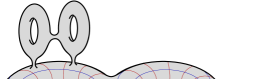
Figure 8. Non-filling transverse pair of multicurves.

By construction, $\mathcal{G}$ is a map in $S^{\prime}$. The vertices of $\mathcal{G}$ are intersections of the multicurves, so all vertices of $\mathcal{G}$ have valence $4$. Hence, all faces of the dual graph $\mathcal{G}^{\ast}$ in $S^{\prime}$ are $4$-gons. The edges of $\mathcal{G}^{\ast}$ dual to horizontal edges of $\mathcal{G}$ will be called vertical, and those dual to the vertical edges of $\mathcal{G}$ will be called horizontal. By construction, any two opposite edges of any face of $\mathcal{G}^{\ast}$ are either both horizontal or both vertical. Realizing the faces of $\mathcal{G}^{\ast}$ as identical metric squares we get a square-tiled surface in the sense of Section 3.

In the case when the transverse pair of multicurves is not filling, we introduce an additional marking of the associated square-tiled surface in order to record the information on the initial surface. We have to mark disjoint collections $\{V_{1,1},\dots,V_{1,j_{1}}\}\sqcup\dots\sqcup\{V_{k,1},\dots,V_{1,j_{k}}\}$ of disjoint vertices of the tiling and genera $g_{1},\dots,g_{k}$ of associated surfaces with respectively $j_{1},\dots,j_{k}$ boundary components. The genus $g$ of the initial surface and the genus $g^{\prime}$ of the associated square-tiled surface are related by

(4.1) $$g=g^{\prime}+(g_{1}+j_{1}-1)+\dots+(g_{k}+j_{k}-1)\,,$$

where $g_{i}+j_{i}-1>0$ for $i=1,\dots,k$. A square-tiled surface endowed with a marking

$$(\{V_{1,1},\dots,V_{1,j_{1}}\},g_{1}),\dots,(\{V_{k,1},\dots,V_{1,j_{k}}\},g_{k})$$

defines the original surface endowed with an ordered connected transverse pair of multicurves uniquely up to a homeomorphism.

We can formalize the above constructions as the following statement.

Proposition 4.1.

There is a natural one-to-one correspondence between filling connected pairs of transverse multicurves on a surface of genus $g$ and square-tiled surfaces of genus $g$ (with non-labeled conical points), where the square tiling is given by the graph $\mathcal{G}^{\ast}$ dual to the graph $\mathcal{G}$ formed by the union of two multicurves.

This correspondence extends to the bijection between non-filling pairs of transverse multicurves and marked square-tiled surfaces (with non-labeled conical points), where the marking satisfies Equation (4.1).

Restricting the correspondence to filling transverse connected pairs of simple closed curves we get a bijection with the subset of square-tiled surfaces of genus $g$ (with non-labeled conical points) having a single horizontal and a single vertical band of squares.

A square-tiled surface carries a meromorphic quadratic differential $q$ with at most simple poles. This quadratic differential has the form $(dz)^{2}$ in the natural coordinate on each square. Simple poles of $q$ correspond to bigons of the complement $S-\mathcal{G}$ (see Definition 1.1); zeroes of degree $m$ correspond to $(4+2m)$-gons. Thus, restricting our consideration to nonorientable connected transverse pairs of multicurves on a surface $S$ of genus $g$, which form exactly $n$ boundary components of the complement $S-\mathcal{G}$ having two edges, we get a quadratic differential in ${\mathcal{Q}}_{g,n}$ in the case when the transverse pair of multicurves is filling (i.e. when $\mathcal{G}$ forms a map) and in ${\mathcal{Q}}_{g^{\prime},n}$ with $g^{\prime}<g$ in the case when the pair is not filling. Specifying the numbers $\mu_{1},\mu_{2},\mu_{3},\dots,\mu_{m},\dots$ of boundary components of the complement $S-\mathcal{G}$ having respectively $6,8,10,\dots,4+2m,\dots$ edges we get square-tiled surfaces in the stratum ${\mathcal{Q}}(\mu,(-1)^{n})$.

Starting from a positively oriented transverse pair of multicurves and applying the construction as above, we get an Abelian square-tiled surface endowed with an Abelian differential $\omega$ having the form $dz$ in the natural coordinate on each square. This time the boundary components of the connected domains obtained by removing the union of the transverse pair of multicurves from the surface have $4,8,12,\dots$ edges. Specifying the numbers $\mu_{1},\mu_{2},\mu_{3},\dots,\mu_{m},\dots$ of boundary components of the complement $S-\mathcal{G}$ having respectively $8,12,\dots,4+4m,\dots$ edges we get square-tiled surfaces in the stratum $\mathcal{H}(\mu)$. The Proposition below is an analog of Proposition 4.1.

Proposition 4.2.

There is a natural one-to-one correspondence between filling oriented transverse connected pairs of multicurves on a surface of genus $g$ and Abelian square-tiled surfaces of genus $g$ (with non-labeled conical points), where the square tiling is given by the graph $\mathcal{G}^{\ast}$ dual to the graph $\mathcal{G}$ formed by the union of two multicurves.

This correspondence extends to the bijection between non-filling oriented transverse pairs of multicurves and marked Abelian square-tiled surfaces (with non-labeled conical points), where the marking satisfies Equation (4.1).

Restricting the correspondence to filling oriented transverse connected pairs of simple closed curves we get a bijection with the subset of Abelian square-tiled surfaces of genus $g$ (with non-labeled conical points) having a single horizontal and a single vertical band of squares.

We are ready now to present our first counting result.

Proposition 4.3.

For any fixed $g$ and $n$ satisfying $2g+n\geq 4$ consider transverse connected pairs of multicurves with at most $2N$ crossings on a surface $S$ of genus $g$, such that the corresponding graph $\mathcal{G}$ forms at most $n$ two-edges boundary components of the complement $S-\mathcal{G}$.

The total number of pairs as above which satisfy any of the following properties:

1. the pair is not filling;

2. the pair is orientable (can take place only when $n=0$);

3. at least one of the boundary components of the complement $S-\mathcal{G}$ has more than six edges;

is of order $o(N^{6g-6+2n})$ as $N\to\infty$.

The number $\operatorname{G}^{\textrm{filling}}_{g,n}(N)$ of filling pairs as above which do not satisfy any of the properties (1)–(3) has the following asymptotics:

(4.2) $$\operatorname{G}^{\textrm{filling}}_{g,n}(N)=\frac{\operatorname{Vol}{\mathcal{Q}}_{g,n}}{(4g-4+n)!\cdot n!\cdot(12g-12+4n)}\cdot N^{6g-6+2n}+o(N^{6g-6+2n})\quad\mbox{ as }N\to\infty\,.$$

Proof.

Suppose that a pair of multicurves as above does not satisfy any of the properties (1)–(3). Then by Proposition (4.1) the number $\operatorname{G}^{\textrm{filling}}_{g,n}(N)$ counts square-tiled surfaces with non-labeled zeroes and poles in the stratum ${\mathcal{Q}}(1^{4g-4+n},(-1)^{n})$ of meromorphic quadratic differentials. There are $(4g-4+n)!\cdot n!$ ways to label $(4g-4+n)$ zeroes and $n$ poles, so Equation (4.2) follows from (3.1).

Suppose that a pair of multicurves is orientable (this implies that $n=0$). Such a pair defines an Abelian square-tiled surface, that represents a point in one of the finite number of strata $\mathcal{H}_{g^{\prime}}$, where $g^{\prime}\leq g$. The number of square-tiled surfaces tiled with at most $2N$ squares in any given stratum $\mathcal{H}(\mu)$ grows as $const\cdot N^{d}$ as $N\to\infty$, where $d=\dim_{\mathbb{C}}\mathcal{H}(\mu)$. Any stratum of Abelian differentials in genus $g^{\prime}\leq g$ has dimension bounded from above by the dimension $\dim_{\mathbb{C}}\mathcal{H}_{g}=4g-3$ of $\mathcal{H}_{g}$. The inequality $2g+n\geq 4$ implies that $4g-3<6g-6+n$. This proves, that the number of filling orientable pairs is negligible compared to the number $\operatorname{G}^{\textrm{filling}}_{g,n}(N)$ of nonorientable filling pairs computed above as $N\to\infty$.

Similarly, if the pair is filling, nonorientable, but at least one of the faces has more than six edges, then the associated square-tiled surface lives in one of the finite number of strata ${\mathcal{Q}}(\mu,(-1)^{n})$ of meromorphic quadratic differentials in ${\mathcal{Q}}_{g,n}$, different from the principal stratum. The number of square-tiled surfaces tiled with at most $2N$ squares in a stratum ${\mathcal{Q}}(\mu,(-1)^{n})$ grows as $const\cdot N^{d}$ as $N\to\infty$, where $d=\dim_{\mathbb{C}}{\mathcal{Q}}(\mu,(-1)^{n})$. The dimension of any stratum in ${\mathcal{Q}}_{g,n}$ different from the principal stratum ${\mathcal{Q}}(1^{4g-4+n},(-1)^{n})$ is strictly less than $\dim_{\mathbb{C}}{\mathcal{Q}}_{g,n}=6g-6+2n$. This proves, that the number of filling nonorientable pairs having at least one of the faces with more than six edges is negligible compared to the number $\operatorname{G}^{\textrm{filling}}_{g,n}(N)$ of nonorientable filling pairs computed above.

It remains to prove that the number of non-filling pairs as above is negligible. Equation (4.1) implies that there is a finite number of choices of parameters $k$ and $g^{\prime},g_{1},j_{1},\dots,g_{k},j_{k}$. Thus, it is sufficient to prove the statement under assumption that all these parameters are fixed, which we impose from now on. The dimensional arguments as above allow to restrict consideration to the situation when the resulting square-tiled surface belongs to the principal stratum ${\mathcal{Q}}(1^{4g^{\prime}-4+n},(-1)^{n})$.

The total number $v$ of vertices of any square-tiled surface of genus $g^{\prime}$ with exactly $k$ squares satisfies the Euler characteristic relation $k-2k+v=2-2g^{\prime}$. Thus, when the number of squares is at most $2N$, the number of choices for any $V_{i,j}$ is at most $2N+2$. Thus, the number of choices of all marked points has the order $const_{1}\cdot N^{J}$, where $J=j_{1}+\dots+j_{k}$, as $N\to\infty$. The number of square-tiled surfaces in the stratum ${\mathcal{Q}}(1^{4g^{\prime}-4+n},(-1)^{n})$ tiled with at most $2N$ squares grows as $const_{2}\cdot N^{6g^{\prime}-6+2n}$ as $N\to\infty$. This implies that the total number of marked square-tiled surfaces tiled with at most $2N$ squares is bounded by $const_{3}\cdot N^{6g^{\prime}-6+2n+J}$ as $N\to\infty$.

Let $G=g_{1}+\dots+g_{k}$. Recall that the entries of Equation (4.1) satisfy the conditions $g_{i}+j_{i}-1>0$ for $i=1,\dots,k$. This implies that $G+J-k\geq k$. Equation (4.1) implies that

$$6g-6+2n=(6g^{\prime}-6+2n+J)+G-k+5(G+J-k)\,.$$

Since $G\geq 0$ and by assumption $k\geq 1$ we conclude that

$$(6g^{\prime}-6+2n+J)=6g-6+2n-(G-k+5(G+J-k))\\ \leq 6g-6+2n-(-k+5k)\leq 6g-6+2n-4\,.$$

Taking into consideration the asymptotic relation (4.2), which we have already proved, this completes the proof of Proposition 4.3. ∎

The statement below is completely analogous:

Proposition 4.4.

For any fixed $g\geq 1$ consider transverse connected oriented pairs of multicurves with at most $N$ crossings on a surface $S$ of genus $g$.

The total number of pairs as above which satisfy any of the following two properties:

1. the pair is not filling;

2. at least one of the boundary components of the complement $S-\mathcal{G}$ has more than $8$ edges;

is of order $o(N^{4g-3})$ as $N\to\infty$.

The number $\operatorname{G}^{+,\textrm{filling}}_{g}(N)$ of filling pairs as above which do not satisfy any of the properties (1)–(2) has the following asymptotics:

(4.3) $$\operatorname{G}^{+,\textrm{filling}}_{g}(N)=\frac{\operatorname{Vol}\mathcal{H}_{g}}{(2g-2)!\cdot(8g-6)}\cdot N^{4g-3}+o(N^{4g-3})\quad\mbox{ as }N\to\infty\,.$$

5. Proofs of the main result for fixed values of $g$ and $n$

In this Section we derive part of the main results of Section 2 from the count presented in Section 3.

Proof of relations (2.1) and (2.2) from Theorem 2.5.

By Proposition 4.1 nonorientable filling meanders on a surface of genus $g$ with at most $2N$ intersections having exactly $n$ bigonal faces and no faces with more than $6$ edges are in the natural one-to-one correspondence with square-tiled surfaces in the stratum ${\mathcal{Q}}(1^{4g-4+n},(-1)^{n})$ tiled with at most $2N$ squares, with non-labeled zeroes and poles, and having a single horizontal and a single vertical cylinder. The number of such square-tiled surfaces with labeled zeroes and poles is given by Formula (3.9) from Theorem 3.3. Dividing both sides of (3.9) by the number $(4g-4+n)!\cdot n!$ of different labelings we get the number of unlabeled square-tiled surfaces as above, i.e. the number $\operatorname{M}^{\textrm{filling}}_{g,n}(N)$ of nonorientable filling meanders with $n$ bigonal and with $4g-4+n$ hexagonal faces, and with no faces of more than $6$ edges

$$\operatorname{M}^{\textrm{filling}}_{g,n}(N)=C_{g,n}N^{6g-6+2n}+o(N^{6g-6+2n})\quad\mbox{ as }N\to\infty\,,$$

with $C_{g,n}$ given by Equation (2.2). Proposition 4.3 implies that all but negligible (as $N\to+\infty$) part of meanders as above are nonorientable, filling, and have only bigonal, quadrangular and hexagonal faces, or, equivalently,

$$\operatorname{M}_{g,n}(N)=\operatorname{M}^{\textrm{filling}}_{g,n}(N)+o(N^{6g-6+2n})\quad\text{ as }N\to\infty\,.$$

This completes the proof of (2.1). Expression (2.3) for $cyl_{1,1}({\mathcal{Q}}_{g,n})$ corresponds to Equation (3.10) from Theorem 3.3. ∎

The proof of the part of Theorem 2.7 which concerns any fixed $g$ (i.e. existence polynomial asymptotics (2.6) and the fact that the coefficient of the leading term is given by expression (2.7)) is completely analogous and is based on Theorem 3.4 and Proposition 4.4. The value of $cyl_{1,1}(\mathcal{H}_{g})$ is given by Formula (3.10), the value of $cyl_{1}(\mathcal{H}_{g})$ is given by Formula (3.7).

Proof of Theorem 2.9.

Gluing the two boundary components in such a way that the endpoints of a balanced arc system are matched, we get a connected transverse pair of multicurves. The horizontal multicurve has a single connected component: it is a simple closed curve represented by the original boundary component, whereas the vertical multicurve may have several connected components. All such transverse connected pairs of multicurves correspond to square-tiled surfaces with unlabeled zeroes and poles having a single horizontal band of squares. Those, which represent meanders, correspond to square-tiled surfaces with unlabeled zeroes and poles having a single horizontal and a single vertical band of squares. Once again Proposition 4.2 allows us to limit our consideration to only those pairs of multicurves of each of the two types which are nonorientable, filling and do not have faces with more than $6$ edges. This implies that

$$\lim_{N\to\infty}\operatorname{P}_{g,n}(N)=\lim_{N\to\infty}\frac{\operatorname{card}(\mathcal{ST}^{\mathit{unlabeled}}_{1,1}({\mathcal{Q}}(1^{4g-4+n},(-1)^{n}),2N))}{\operatorname{card}(\mathcal{ST}^{\mathit{unlabeled}}_{1}({\mathcal{Q}}(1^{4g-4+n},(-1)^{n}),2N))}\,.$$

Since, passing from the count of unlabeled square-tiled surfaces to the count of labeled ones, we have to label the same number of zeroes and poles for the square-tiled surfaces in the numerator and in the denominator, we get the same limit for the ratio of the numbers of analogous labeled square-tiled surfaces. Combining Equations (3.4),(3.9) and (3.10) we get

$$\lim_{N\to\infty}\frac{\operatorname{card}(\mathcal{ST}^{\mathit{labeled}}_{1,1}({\mathcal{Q}}(1^{4g-4+n},(-1)^{n}),2N))}{\operatorname{card}(\mathcal{ST}^{\mathit{labeled}}_{1}({\mathcal{Q}}(1^{4g-4+n},(-1)^{n}),2N))}=\frac{cyl_{1}({\mathcal{Q}}_{g,n})}{\operatorname{Vol}{\mathcal{Q}}_{g,n}}\,,$$

which proves (2.9) and (2.10). ∎

The part of Theorem 2.12 claiming existence of the limit (2.14) and providing expression (2.15) for its value is proved completely analogously.

The large $n$ and large $g$ asymptotics of the related constants are given in Corollary 6.7, Corollary 6.9 and Corollary 6.10 of Section 6.

Proof of Theorem 2.10.

Having been translated into the language of square-tiled surface, Theorem 2.10 becomes an implication of Proposition 4.3 combined with Corollaries 4.24 and 4.25 from [DGZZ2]. For the sake of completeness we justify below that all topological configurations of filling nonorientable systems of arcs mentioned in Theorem 2.10 are realizable.

We start with the case when the surface of genus $g-1$ has two boundary components. If $g=1$, the proof of existence of a filling nonorientable system of arcs having $n_{1}$ minimal arcs at the first boundary component and $n_{2}$ minimal arcs at the second boundary component is trivial for any pair $n_{1},n_{2}\in\mathbb{N}$. Thus, we can suppose that $g\geq 2$.

Lemma 5.1.

An orientable surface of any genus greater than or equal to one with exactly two boundary components admits a nonorientable filling balanced system of arcs such that all faces of the complement are hexagons.

We present an equivalent formulation of this Lemma suitable for technique of Corollaries 4.24 and 4.25 from [DGZZ2].

Lemma 5.2.

For any $g\geq 2$ the stratum ${\mathcal{Q}}(1^{4g-4})$ admits a one-cylinder separatrix diagram such that the singular leaf is connected.

Proof.

One can use the diagram from [Zor3, Figure 13] for $g=2$ and the diagram from [Zor3, Figure 14] for $g\geq 3$ letting in both cases $p=0$ (where $p$ is defined in the Figures). ∎

We will need the following observation. Note that the original system of arcs, constructed in Lemma 5.1 is nonorientable. It means that it contains at least one arc coming back to the same boundary component. If there is an arc at one boundary component, there should be at least one arc having both endpoints on the other boundary component since the system is balanced.

Having constructed a system of arcs as in Lemma 5.1 we can complete it with arbitrary number $n_{1}$ of minimal arcs at the first boundary component and with arbitrary number $n_{2}$ of minimal arcs at the second boundary component. If $n_{1}\neq n_{2}$, the resulting system of arcs is not balanced, but since each of the boundary components has an arc with both endpoints on this boundary component, taking several copies of such an arc for the component with deficiency of endpoints we get already a balanced systems. By construction it is nonorientable and filling. If some of the faces have more than 6 sides, we can add extra arcs to partition them to get only bigons, quadrilaterals and hexagons. The proof of existence of balanced arc systems on a connected surface with two boundary components mentioned in Theorem 2.10 is completed. The proof of existence of remaining arc systems mentioned in Theorem 2.10 is trivial. ∎

Remark 5.3.

The technique of the above proofs applies without any further changes to meandric systems. Meandric systems correspond to square-tiled surfaces having a certain number of horizontal bands of squares and a certain number of vertical bands of squares, see Section 4 of the original paper [DGZZ2] for more details.

Proof of Lemma 2.6.

One can easily construct a meander with $2N$ crossings on a surface of genus $g$ from a meander with $2N$ crossings on a sphere by replacing a topological disk, forming a face of the graph $\mathcal{G}$, by a topological surface of genus $g$ having a single boundary component. This gives an obvious lower bound $M_{0}^{=N}$ for $M_{g}^{=N}$. The number $M_{0}^{=N}$ is greater than $C_{N}$, see [LZv1] (the paper [AlP], actually, provides a sharper bound).

For the upper bound, we first assume that the meander is filling, as it was done above. Cutting along one of the two closed curves forming the meander we get a filling balanced arc system of genus $g$ with $2N$ endpoints on each boundary component. We first consider the case, when we get two connected components of genera $g_{1}$ and $g_{2}$, where $g_{1}+g_{2}=g$. The dual graph $\mathcal{G}^{*}$ of the arc system on each component is a unicellular map with $N$ edges: the unique face corresponds to the boundary of the cut component. The number $\varepsilon_{g}(N)$ of unicellular maps with $N$ edges on a genus $g$ surface is well-known (see [HrZa, Theorem 2] or [CFF, Theorem 5 and Proposition 6]):

$$\varepsilon_{g}(N)=C_{N}\cdot p_{g}(N)\,,$$

where $p_{g}$ is an explicit polynomial of degree $3g$. The number of meanders in that case is then bounded by $2N\sum_{g_{1}+g_{2}=g}\varepsilon_{g_{1}}(N)\varepsilon_{g_{2}}(N)\leq{C_{N}}^{2}P_{g}(N)$ where $P_{g}(N)=2N\sum_{g_{1}+g_{2}=g}p_{g_{1}}(N)p_{g_{2}}(N)$ is of degree $3g+1$ and the factor $2N$ accounts for the $2N$ possibly different identifications.

In the second case we get a single connected surface with two boundary components. Now the dual graph $\mathcal{G}^{*}$ to the arc system is a bicellular map of genus $g-1$ with $2N$ edges: the two faces of the graph correspond to the two boundary components of the surface. The number $\varepsilon^{[2]}_{g-1}(N)$ of such bicellular maps is bounded by

$$\varepsilon_{g-1}^{[2]}(2N)\leq\varepsilon_{g}(2N+1)=C_{2N+1}\cdot p_{g}(2N+1)\,,$$

see [HR, Corrolary 1]. The number of meanders in that case is bounded by $2N\cdot p_{g}(2N+1)\cdot C_{2N+1}$, where the factor $2N$ accounts for the $2N$ possibly different identifications.

By Stirling’s approximation we have

$$(C_{N})^{2}\sim\frac{1}{\pi}\cdot N^{-3}\cdot 2^{4N}\,,\quad C_{2N+1}\sim\sqrt{\frac{2}{\pi}}\cdot N^{-3/2}\cdot 2^{4N}\,.$$

Recall that the polynomial $P_{g}(N)$ has degree $3g+1$ and the polynomial $p_{g}(2N+1)$ has degree $3g$ in $N$. Hence, the quantity $P_{g}(N)\cdot(C_{N})^{2}$ is negligible compared to $2N\cdot p_{g}(2N+1)\cdot C_{2N+1}$ as $N\to\infty$.

The above estimates imply that the contributions of non-filling meanders are negligible compared to $2N\cdot p_{g}(2N+1)\cdot C_{2N+1}$, since the corresponding dual maps have lower genera.

The rough upper and lower bounds obtained above can be improved using finer arguments. We do not do it here to avoid overloading of the paper. ∎

6. Asymptotic count for large values of $g$ and $n$

6.1. Formula for the Masur–Veech volume through intersection numbers

We recall here the formula from [DGZZ3] giving the Masur–Veech volume $\operatorname{Vol}{\mathcal{Q}}_{g,n}$ of the moduli spaces ${\mathcal{Q}}_{g,n}$ of meromorphic quadratic differentials with $n$ simple poles on Riemann surfaces of genus $g$.

A multicurve on a surface of genus $g$ with $n$ punctures cuts the surface into several connected components, where each component has certain genus, certain number of boundary components and certain number of punctures. By a stable graph we call the dual graph to such a multicurve, decorated with the following information: to each vertex of the graph we associate the genus of the corresponding connected component, and for each puncture on that component we add a half edge at the corresponding vertex. These graphs encode the topological type of a multicurve. Using a similar correspondence as the one described in Section 4, one can show that these graphs encode also the type of decomposition into cylinders of a square-tiled surface.

We are particularly interested in stable graphs representing simple closed curves (or, equivalently, one-cylinder square-tiled surfaces). A stable graph $\Gamma_{1}(g,n)$, as on the left in Figure 9, represents a non-separating simple closed curve on a surface of genus $g$ with $n$ punctures. Considering stable graphs $\Gamma_{1}(g,n)$ we always assume that $g\geq 1$ and that if $g=1$, then $n\geq 1$ without specifying it explicitly. A stable graph $\Gamma_{g_{1},n_{1}}^{g_{2},n_{2}}$, as on the right in Figure 9, represents a simple closed curve separating the surface into a subsurface of genus $g_{1}$ endowed with $n_{1}$ punctures and a complementary subsurface of genus $g_{2}$ endowed with $n_{2}$ punctures. Here $g=g_{1}+g_{2}$ and $n=n_{1}+n_{2}$. Considering the graphs $\Gamma_{g_{1},n_{1}}^{g_{2},n_{2}}$ we will always assume that $2g_{i}+n_{i}\geq 3$ for $i=1,2$, without specifying it explicitly. We denote by $\mathcal{G}_{g,n}$ the set of all stable graphs corresponding to a surface of genus $g$ with $n$ punctures.

Figure 9. Stable graphs representing a non-separating (on the left) and separating (on the right) simple closed curves.

Let $g,n$ be non-negative integers with $2g+n\geq 3$. Let $b_{1}$, …, $b_{n}$ be formal variables. For a multi-index $\boldsymbol{d}=(d_{1},\ldots,d_{n})$ we denote by $b^{2\boldsymbol{d}}$ the product $b_{1}^{2d_{1}}\cdot\cdots\cdot b_{n}^{2d_{n}}$, by $|\boldsymbol{d}|$ the sum $d_{1}+\cdots+d_{n}$ and by $\boldsymbol{d}!$ the product $d_{1}!\cdots d_{n}!$

Define a homogeneous polynomial $N_{g,n}(b_{1},\dots,b_{n})$ of degree $6g-6+2n$ in the variables $b_{1},\dots,b_{n}$ as

(6.1) $$N_{g,n}(b_{1},\dots,b_{n})=\sum_{|\boldsymbol{d}|=3g-3+n}c_{\boldsymbol{d}}b^{2\boldsymbol{d}}\,,$$

where

$$c_{\boldsymbol{d}}=\frac{1}{2^{5g-6+2n}\,\boldsymbol{d}!}\,\int_{\overline{\mathcal{M}}_{g,n}}\psi_{1}^{d_{1}}\dots\psi_{n}^{d_{n}}.$$

Here $\psi_{1}$, …, $\psi_{n}$ are the $\psi$-classes on the Deligne–Mumford compactification $\overline{\mathcal{M}}_{g,n}$.

We also use the following common notation for the intersection numbers as above (often called Witten–Kontsevich correlators). Given an ordered partition $d_{1}+\dots+d_{n}=3g-3+n$ of $3g-3+n$ into a sum of non-negative integers we define

$$\langle\tau_{d_{1}}\dots\tau_{d_{n}}\rangle_{g}:=\int_{\overline{\mathcal{M}}_{g,n}}\psi_{1}^{d_{1}}\dots\psi_{n}^{d_{n}}\,.$$

Polynomials $N_{g,n}$ are implicitly present in Kontsevich’s proof [Kon] of Witten’s conjecture [Wi] and in the discretized model of the moduli space of L. Chekhov, see [Ch1, Ch2]. They represent the top homogeneous parts of Norbury’s quasi-polynomials counting metric ribbon graphs with edges of integer lengths [Nb]. Up to a normalization constant $2^{2g-3+n}$, the polynomial $N_{g,n}(b_{1},\dots,b_{n})$ coincides with the top homogeneous part of Mirzakhani’s volume polynomial $V_{g,n}(b_{1},\dots,b_{n})$ providing the Weil–Petersson volume of the moduli space of bordered Riemann surfaces [Mi1].

Given a stable graph $\Gamma$ denote by $V(\Gamma)$ the set of its vertices and by $E(\Gamma)$ the set of its edges. To each stable graph $\Gamma\in\mathcal{G}_{g,n}$ we associate the following homogeneous polynomial $P_{\Gamma}$ of degree $6g-6+2n$. To every edge $e\in E(\Gamma)$ we assign a formal variable $b_{e}$. Given a vertex $v\in V(\Gamma)$ denote by $g_{v}$ the integer number decorating $v$ and denote by $n_{v}$ the valency of $v$, where the legs adjacent to $v$ are counted towards the valency of $v$. Take a small neighborhood of $v$ in $\Gamma$. We associate to each half-edge (“germ” of edge) $e$ adjacent to $v$ the monomial $b_{e}$; we associate $0$ to each leg. We denote by $\boldsymbol{b}_{v}$ the resulting collection of size $n_{v}$. If some edge $e$ is a loop joining $v$ to itself, $b_{e}$ would be present in $\boldsymbol{b}_{v}$ twice; if an edge $e$ joins $v$ to a distinct vertex, $b_{e}$ would be present in $\boldsymbol{b}_{v}$ once; all the other entries of $\boldsymbol{b}_{v}$ correspond to legs; they are represented by zeroes. To each vertex $v\in E(\Gamma)$ we associate the polynomial $N_{g_{v},n_{v}}(\boldsymbol{b}_{v})$, where $N_{g,v}$ is defined in (6.1). We associate to the stable graph $\Gamma$ the polynomial obtained as the product $\prod b_{e}$ over all edges $e\in E(\Gamma)$ multiplied by the product $\prod N_{g_{v},n_{v}}(\boldsymbol{b}_{v})$ over all $v\in V(\Gamma)$. We define $P_{\Gamma}$ as follows:

$$P_{\Gamma}(\boldsymbol{b})=\frac{2^{6g-5+2n}\cdot(4g-4+n)!}{(6g-7+2n)!}\cdot\frac{1}{2^{|V(\Gamma)|-1}}\cdot\frac{1}{|\operatorname{Aut}(\Gamma)|}\cdot\prod_{e\in E(\Gamma)}b_{e}\cdot\prod_{v\in V(\Gamma)}N_{g_{v},n_{v}}(\boldsymbol{b}_{v})\,.$$

Example 6.1.

Using the rule described above we get the following polynomials associated to the graphs $\Gamma_{1}(g,n)$ and $\Gamma_{g_{1},n_{1}}^{g_{2},n_{2}}$ from Figure 9.

(6.2) $$P_{\Gamma_{1}(g,n)}(b) =\frac{2^{6g-5+2n}\cdot(4g-4+n)!}{(6g-7+2n)!}\cdot\frac{1}{2}\cdot b_{1}\cdot N_{g-1,n+2}(b_{1},b_{1},0,\dots,0)\,,$$

(6.3) $$P_{\Gamma_{g_{1},n_{1}}^{g_{2},n_{2}}}(b_{1}) =\frac{2^{6g-5+2n}\cdot(4g-4+n)!}{(6g-7+2n)!}\cdot\frac{1}{2|\operatorname{Aut}(\Gamma_{g_{1},n_{1}}^{g_{2},n_{2}})|}$$

$$\times b_{1}\cdot N_{g_{1},n_{1}+1}(b_{1},0,\dots,0)\cdot N_{g_{2},n_{2}+1}(b_{1},0,\dots,0)\,.$$

Here we used the fact that $|\operatorname{Aut}(\Gamma_{1}(g,n))|=2$ for any $g$ and $n$. We have

(6.4) $$|\operatorname{Aut}(\Gamma_{g_{1},n_{1}}^{g_{2},n_{2}})|=\begin{cases}2&\text{when we have both}\ g_{1}=g_{2}\text{ and }n_{1}=n_{2}\,;\\ 1&\text{otherwise}\,.\end{cases}$$

We now define an operator $\mathcal{Z}$ acting on polynomials. It is defined on monomials as

(6.5) $$\mathcal{Z}\ :\quad\prod_{i=1}^{k}b_{i}^{m_{i}}\longmapsto\prod_{i=1}^{k}\big{(}m_{i}!\cdot\zeta(m_{i}+1)\big{)}\,,$$

and extended to arbitrary polynomials by linearity. Everywhere in the current paper $\zeta$ is the Riemann zeta function

$$\zeta(s)=\sum_{n\geq 1}\frac{1}{n^{s}}\,.$$

We have proved in [DGZZ3] the following statement.

Theorem ([DGZZ3, Theorem 1.5]).

The Masur–Veech volume $\operatorname{Vol}{\mathcal{Q}}_{g,n}$ of the moduli space of meromorphic quadratic differentials with $n$ simple poles on complex curves of genus $g$ has the following value:

(6.6) $$\operatorname{Vol}{\mathcal{Q}}_{g,n}=\sum_{\Gamma\in\mathcal{G}_{g,n}}\operatorname{Vol}(\Gamma)\,,$$

where the contribution of an individual stable graph $\Gamma$ is equal to

(6.7) $$\operatorname{Vol}(\Gamma)=\mathcal{Z}(P_{\Gamma})\,.$$

6.2. Contribution of single-band square-tiled surfaces

In this section we analyze the contributions $\operatorname{Vol}(\Gamma_{1}(g,n))$ and $\operatorname{Vol}(\Gamma_{g1,n1}^{g_{2},n_{2}})$ of the graphs representing square-tiled surfaces having a single horizontal cylinder to the Masur–Veech volume $\operatorname{Vol}{\mathcal{Q}}_{g,n}$ expressed as a sum in the right-hand side of Equation (6.6). We start with preparatory facts on Witten–Kontsevich correlators involved in the polynomials $P_{\Gamma_{1}(g,n)}$ and $P_{\Gamma_{g1,n1}^{g_{2},n_{2}}}$; see Equations (6.2) and (6.3) respectively.

Lemma 6.2.

For $g\geq 1$, $n\geq 0$, $d_{1}\geq 0$, the intersection numbers satisfy the following equalities:

(6.8) $$\langle\tau_{0}^{n}\tau_{3g+n-2}\rangle_{g} = \langle\tau_{3g-2}\rangle_{g}=\frac{1}{24^{g}\cdot g!}\,.$$

(6.9) $$\langle\tau_{0}^{n+2}\tau_{n}\rangle_{0} = 1\,.$$

(6.10) $$\qquad\langle\tau_{0}^{n}\tau_{d_{1}}\tau_{3g-1+n-d_{1}}\rangle_{g} = \sum_{i=\max(0,d_{1}-3g+1)}^{\min(d_{1},n)}\binom{n}{i}\langle\tau_{d_{1}-i}\tau_{3g-1-d_{1}+i}\rangle_{g}\,.$$

(6.11) $$\langle\tau_{0}^{n}\tau_{d_{1}}\tau_{n-1-d_{1}}\rangle_{0} = \binom{n-1}{d_{1}}\,.$$

Proof.

Applying repeatedly the string equation

$$\langle\tau_{0}\tau_{d_{1}}\dots\tau_{d_{k}}\rangle_{g}=\sum_{i=1}^{k}\langle\tau_{d_{1}}\dots\tau_{d_{i}-1}\dots\tau_{d_{k}}\rangle_{g}$$

we eliminate $\tau_{0}$ thus proving the left equality in (6.8) and Equation (6.10). The right equality in (6.8) is due to E. Witten [Wi]. The remaining equalities concern genus $0$ correlators, for which we use the closed formula

$$\langle\prod_{i=1}^{n}\tau_{d_{i}}\rangle_{0}=\frac{(n-3)!}{\prod_{i}d_{i}!}\,.$$

also due to E. Witten [Wi, p. 251, after Equation (2.26)]. ∎

Values of 2-correlators $\langle\tau_{k}\tau_{3g-1-k}\rangle_{g}$ can be obtained in a particularly efficient way through the following recursive relations found in [Zog1]:

(6.12) $$(6j+1)\langle\tau_{3j}\tau_{3g-1-3j}\rangle_{g}-(6j+1-6j)\langle\tau_{3j-1}\tau_{3g-3j}\rangle_{g}=\frac{1}{24^{g}\cdot g!}\binom{g}{j}\left(1-\frac{2j}{g}\right)\,.$$

(6.13) $$(6j+3)\langle\tau_{3j+1}\tau_{3g-2-3j}\rangle_{g}-(6j-1-6j)\langle\tau_{3j}\tau_{3g-1-3j}\rangle_{g}=-2\cdot\frac{1}{24^{g}\cdot g!}\binom{g-1}{j}\,.$$

(6.14) $$(6j+5)\langle\tau_{3j+2}\tau_{3g-3-3j}\rangle_{g}-(6j-3-6j)\langle\tau_{3j+1}\tau_{3g-2-3j}\rangle_{g}=2\cdot\frac{1}{24^{g}\cdot g!}\binom{g-1}{j}\,.$$

Here we use the explicit formula (6.8) for $\langle\tau_{0}\tau_{3g-1}\rangle_{g}=\frac{1}{24^{g}\cdot g!}$ as the base of the recursion. In genera $1$ and $2$ this gives $\langle\tau_{1}\tau_{1}\rangle=\frac{1}{24}$ and $\langle\tau_{1}\tau_{4}\rangle=\frac{1}{384}$, $\langle\tau_{2}\tau_{3}\rangle=\frac{29}{5760}$. The remaining correlators in $g=1,2$ are obtained by the symmetry $\langle\tau_{3g-1-k}\tau_{k}\rangle_{g}=\langle\tau_{k}\tau_{3g-1-k}\rangle_{g}$ for $k=0,\dots,3g-1$.

We denote by $c_{1}(\Gamma)=\operatorname{Vol}(\Gamma)$ the contribution of square-tiled surfaces associated to a stable graph $\Gamma$ to the Masur–Veech volume $\operatorname{Vol}{\mathcal{Q}}_{g,n}$, see Equation (6.6). Graphs $\Gamma_{1}(g,n)$ and $\Gamma_{g_{1},n_{1}}^{g_{2},n_{2}}$ as in Figure 9 are the only stable graphs in $\mathcal{G}_{g,n}$ having a single edge (which we distinguish from $n$ legs). In other words, these are the only graphs representing $1$-cylinder square-tiled surfaces. Among all $1$-cylinder square-tiled surfaces associated to these stable graphs, we distinguish those for which the single horizontal cylinder is composed from a single-band of squares and we can compute separately the contribution $cyl_{1}(\Gamma)$ of such square-tiled surfaces to the Masur–Veech volume $\operatorname{Vol}{\mathcal{Q}}_{g,n}$.

Lemma 6.3.

The contributions of single-band square-tiled surfaces to the volume of the principal strata ${\mathcal{Q}}_{g,n}$ are given by

(6.15) $$cyl_{1}(\Gamma_{1}(g,n)) =2^{g+1}\frac{(4g-4+n)!}{(3g-4+n)!}\cdot\sum_{d_{1}=0}^{3g-4+n}\binom{3g-4+n}{d_{1}}\langle\tau_{0}^{n}\tau_{d_{1}}\tau_{3g-4+n-d_{1}}\rangle_{g-1}$$

(6.16) $$cyl_{1}(\Gamma_{g_{1},n_{1}}^{g_{2},n_{2}}) =\frac{2^{g+2}}{|\operatorname{Aut}(\Gamma_{g_{1},n_{1}}^{g_{2},n_{2}})|}\cdot\frac{(4g-4+n)!}{(3g-4+n)!}\cdot\frac{1}{g!\cdot 24^{g}}\cdot\binom{g}{g_{1}}\cdot\binom{3g-4+n}{3g_{1}-2+n_{1}},$$

where $g=g_{1}+g_{2}$ and $n=n_{1}+n_{2}$.

The total contribution of single-band square-tiled surfaces to the volume of ${\mathcal{Q}}_{g,n}$ is given by

(6.17) $$cyl_{1}({\mathcal{Q}}_{g,n})=cyl_{1}(\Gamma_{1}(g,n))+\frac{1}{2}\sum_{n_{1}=0}^{n}\binom{n}{n_{1}}\sum_{g_{1}=0}^{g}|\operatorname{Aut}(\Gamma_{g_{1},n_{1}}^{g_{2},n_{2}})|\cdot cyl_{1}(\Gamma_{g_{1},n_{1}}^{g_{2},n_{2}})\,.$$

Proof.

The following relation generalizing (3.5) is valid for any stable graph $\Gamma$ with a single edge and for any $g$ and $n$.

(6.18) $$\operatorname{Vol}(\Gamma)=c_{1}(\Gamma)=cyl_{1}(\Gamma)\cdot\zeta(6g-6+2n)\,.$$

This relation is an immediate corollary of [DGZZ3, Formula (1.14) and Lemma 1.32]. Thus, to prove the desired expressions, it is sufficient to apply the relation $\operatorname{Vol}(\Gamma)=\mathcal{Z}(P_{\Gamma})$ given by (6.7) to the two stable graphs under consideration. The polynomials $P_{\Gamma_{1}(g,n)}(b)$ and $P_{\Gamma_{g_{1},n_{1}}^{g_{2},n_{2}}}(b_{1})$ are given in Equation (6.2) and (6.3), where, applying the general definition (6.1) of the polynomials $N_{g,n}$ we obtain

$$N_{g-1,n+2}(b_{1},b_{2},0,\dots,0) =\frac{1}{2^{5g-7+2n}}\sum_{\begin{subarray}{c}d_{1}+d_{2}=3g-4+n\\ d_{1}\geq 0,\,d_{2}\geq 0\end{subarray}}\frac{\langle\tau_{0}^{n}\tau_{d_{1}}\tau_{d_{2}}\rangle_{g-1}}{d_{1}!d_{2}!}b_{1}^{2d_{1}}b_{2}^{2d_{2}}\,,$$

$$N_{g_{1},n_{1}+1}(b_{1},0,\dots,0) =\frac{1}{2^{5g_{1}-4+2n_{1}}}\frac{\langle\tau_{0}^{n_{1}}\tau_{3g_{1}-2+n_{1}}\rangle_{g_{1}}}{(3g_{1}-2+n_{1})!}b_{1}^{6g_{1}-4+2n_{1}}\,.$$

Plugging the operator $\mathcal{Z}$, defined by (6.5), into the formula (6.7) and simplifying the results using relations (6.8)–(6.11) from Lemma 6.2 we obtain Equations (6.15) and (6.16).

Note that $\Gamma_{g_{1},n_{1}}^{g_{2},n_{2}}$ and $\Gamma_{g_{2},n_{2}}^{g_{1},n_{1}}$ define the same stable graphs. Thus, the stable graph $\Gamma_{g_{1},n_{1}}^{g_{2},n_{2}}$ is present in the sum (6.17) exactly once if and only if both conditions $g_{1}=g_{2}$ and $n_{1}=n_{2}$ are satisfied. All other stable graphs of the form $\Gamma_{g_{1},n_{1}}^{g_{2},n_{2}}$ are present in the sum (6.17) twice. Taking into consideration Equation (6.4), this justifies (6.17). Lemma 6.3 is proved. ∎

The combinatorial Proposition 6.4 below simplifies expressions (6.15) and (6.16) for $cyl_{1}(\Gamma_{1}(g,n))$ and $cyl_{1}(\Gamma_{g_{1},n_{1}}^{g_{2},n_{2}})$ respectively.

Proposition 6.4.

Assume that $g\geq 1$, and that if $g=1$ then $n\geq 2$. The contribution to the Masur–Veech volume of the principal stratum ${\mathcal{Q}}_{g,n}$ of meromorphic quadratic differentials coming from single-band square-tiled surfaces corresponding to the stable graph $\Gamma_{1}(g,n)$ has the following form:

(6.19) $$cyl_{1}(\Gamma_{1}(1,n)) =4n\cdot\binom{2n-2}{n-1}\quad\text{for }g=1\,;$$

(6.20) $$cyl_{1}(\Gamma_{1}(g,n)) =2^{g+1}\binom{4g-4+n}{g}\cdot g!\sum_{k=0}^{3g-4}\binom{3g-4+2n}{n+k}\langle\tau_{k}\tau_{3g-4-k}\rangle_{g-1}\quad\text{for }g\geq 2\,.$$

The total contribution to the Masur–Veech volume of the principal stratum ${\mathcal{Q}}_{g,n}$ of meromorphic quadratic differentials coming from single-band square-tiled surfaces corresponding to all stable graphs $\Gamma_{g_{1},n_{1}}^{g_{2},n_{2}}$ has the following form:

(6.21) $$\frac{1}{2}\binom{n}{n_{1}}\sum_{\begin{subarray}{c}g_{1}+g_{2}=g\\ n_{1}+n_{2}=n\end{subarray}}|\operatorname{Aut}(\Gamma_{g_{1},n_{1}}^{g_{2},n_{2}})|\cdot cyl_{1}(\Gamma_{g_{1},n_{1}}^{g_{2},n_{2}})=2^{g+1}\binom{4g-4+n}{g}\frac{1}{24^{g}}\sum_{g_{1}=0}^{g}\binom{g}{g_{1}}\binom{3g-4+2n}{3g_{1}-2+n}\,.$$

The total contribution of single-band square-tiled surfaces to the volume of ${\mathcal{Q}}_{g,n}$ is given by

(6.22) $$cyl_{1} ({\mathcal{Q}}_{0,n})=2\binom{2n-4}{n-2}\quad\text{for }n\geq 4\,;$$

(6.23) $$cyl_{1} ({\mathcal{Q}}_{1,n})=4n\cdot\binom{2n-2}{n-1}+\frac{n}{3}\cdot\binom{2n-1}{n-2}\quad\text{for }n\geq 2\,;$$

(6.24) $$cyl_{1} ({\mathcal{Q}}_{g,n})=2^{g+1}\binom{4g-4+n}{g}\cdot\Bigg{(}g!\sum_{k=0}^{3g-4}\binom{3g-4+2n}{n+k}\langle\tau_{k}\tau_{3g-4-k}\rangle_{g-1}$$

$$\qquad+\frac{1}{24^{g}}\sum_{g_{1}=0}^{g}\binom{g}{g_{1}}\binom{3g-4+2n}{3g_{1}-2+n}\Bigg{)}\quad\text{for }g\geq 2\,.$$

Proof.

We develop formulas obtained in Lemma 6.3. Using the following combinatorial identity (see [Gd, (3.20)]):

(6.25) $$\sum_{k=0}^{n}\binom{n}{k}\binom{x}{k+r}=\binom{n+x}{n+r}\,.$$

and Equation (6.11), we get for $g=1$

$$\sum_{d_{1}=0}^{3g-4+n}\binom{3g-4+n}{d_{1}}\langle\tau_{0}^{n}\tau_{d_{1}}\tau_{3g-4+n-d_{1}}\rangle_{g-1}=\sum_{d_{1}=0}^{n-1}\binom{n-1}{d_{1}}\binom{n-1}{d_{1}}=\binom{2n-2}{n-1}\,,$$

which simplifies the sum in (6.15) in the case $g=1$.

When $g\geq 2$, using equation (6.10) and letting $k=d_{1}-i$, we get:

$$\sum_{d_{1}=0}^{3g-4+n}\binom{3g-4+n}{d_{1}}\langle\tau_{0}^{n}\tau_{d_{1}}\tau_{3g-4+n-d_{1}}\rangle_{g-1}\\ =\sum_{d_{1}=0}^{3g-4+n}\sum_{i=\max(0,d_{1}-3g+4)}^{\min(d_{1},n)}\binom{3g-4+n}{d_{1}}\binom{n}{i}\langle\tau_{d_{1}-i}\tau_{3g-4-d_{1}+i}\rangle_{g-1}=\\ =\sum_{k=0}^{3g-4}\langle\tau_{k}\tau_{3g-4-k}\rangle_{g-1}\sum_{i=0}^{n}\binom{n}{i}\binom{3g-4+n}{i+k}=\sum_{k=0}^{3g-4}\langle\tau_{k}\tau_{3g-4-k}\rangle_{g-1}\binom{2n+3g-4}{n+k}\,,$$

where we use identity (6.25) one more time to justify the last equation.

Finally, we can simplify the second term in the sum (6.17) from Lemma 6.3 simplifying expression (6.20) for $cyl_{1}(\Gamma_{g_{1},n_{1}}^{g_{2},n_{2}})$ from this Proposition. We get

$$\frac{1}{2}\sum_{n_{1}=0}^{n}\binom{n}{n_{1}}\sum_{g_{1}=0}^{g}|\operatorname{Aut}(\Gamma_{g_{1},n_{1}}^{g_{2},n_{2}})|\cdot cyl_{1}(\Gamma_{g_{1},n_{1}}^{g_{2},n_{2}})=\\ =2^{g+1}\cdot\frac{(4g-4+n)!}{(3g-4+n)!}\cdot\frac{1}{g!\,24^{g}}\sum_{n_{1}=0}^{n}\sum_{g_{1}=0}^{g}\binom{n}{n_{1}}\binom{g}{g_{1}}\binom{3g-4+n}{3g_{1}-2+n_{1}}\,.$$

Changing the order of summation and applying identity (6.25) we can simplify the latter sum as

$$\sum_{g_{1}=0}^{g}\binom{g}{g_{1}}\sum_{n_{1}=0}^{n}\binom{n}{n_{1}}\binom{3g-4+n}{3g_{1}-2+n_{1}}=\sum_{g_{1}=0}^{g}\binom{g}{g_{1}}\binom{3g-4+2n}{3g_{1}-2+n}\,,$$

which justifies (6.21). ∎

Combining proposition 6.4 with recursive formulas (6.12)–(6.14) for 2-correlators we get explicit expressions for $cyl_{1}({\mathcal{Q}}_{g,n})$ in terms of $g$ and $n$. In the next two sections we analyze $cyl_{1}({\mathcal{Q}}_{g,n})$ in two regimes: when $g$ is fixed and $n\to\infty$ and in the regime when $n$ is fixed and $g\to+\infty$.

6.3. Asymptotic count for large values of $n$

We now discuss asymptotics of the quantities $\operatorname{Vol}{\mathcal{Q}}_{g,n}$, $cyl_{1}(\mathcal{Q}_{g,n})$, $c_{1}({\mathcal{Q}}_{g,n})$, representing the Masur–Veech volume, and the contributions to this volume coming from single-band square-tiled surfaces, and from one-cylinder square-tiled surfaces respectively. In this section we study the regime when the genus $g$ is fixed while the number of poles $n$ tends to infinity. This allows us to derive asymptotic of the quantities $cyl_{1,1}({\mathcal{Q}}_{g,n})$ and $\operatorname{P}_{1}({\mathcal{Q}}_{g,n})$ in the same regime and, thus, prove Formula (2.4) from Theorem 2.5.

We start with the following simple Lemma:

Lemma 6.5.

For any positive integer $a\geq 2$ and for any integers $b$ and $c$ one has the following asymptotics:

(6.26) $$\binom{an+b}{n+c}\sim\frac{1}{\sqrt{2\pi n}}\cdot\frac{a^{an+b+\frac{1}{2}}}{{(a-1)}^{(a-1)n+b+\frac{1}{2}}}\quad\text{as }n\to+\infty\,.$$

Proof.

It is sufficient to prove the Lemma for particular case $c=0$ since then, given arbitrary $c$ we denote $n+c$ by $m$ and apply the asymptotic formula for $\binom{am+(b-ac)}{m}$.

For $c=0$ we apply Stirling’s formula to each of the three factorials in $\binom{an+b}{n}=\frac{(an+b)!}{((a-1)n+b)!\cdot n!}$ and having simplified the resulting expression we get (6.26). ∎

Corollary 6.6.

For any fixed genus $g\geq 0$, we have the following asymptotics:

(6.27) $$cyl_{1}(\mathcal{Q}_{g,n})\sim c_{1}({\mathcal{Q}}_{g,n})\sim\frac{1}{\sqrt{\pi}}\cdot a_{g}\cdot n^{g-\frac{1}{2}}\cdot 4^{n}\quad\text{as }n\to\infty\,,$$

where $a_{0}=\cfrac{1}{8}$, $a_{1}=\cfrac{7}{6}$ and

(6.28) $$a_{g}=2^{2g-3}\cdot\left(2^{2g}\sum_{k=0}^{3g-4}\langle\tau_{k}\tau_{3g-4-k}\rangle_{g-1}+\frac{1}{3^{g}g!}\right)\text{ for }g\geq 2\,.$$

Proof.

A computation for $g=0$ is, essentially, performed in [DGZZ2]. Namely, by Formula (1.5) in [DGZZ2] one has

$$p_{1}({\mathcal{Q}}(1^{n-4},-1^{n}))=\frac{cyl_{1}({\mathcal{Q}}(1^{n-4},-1^{n}))}{\operatorname{Vol}{\mathcal{Q}}(1^{n-4},-1^{n})}\,.$$

Since ${\mathcal{Q}}(1^{n-4},-1^{n})$ is the unique stratum of top dimension in the moduli space ${\mathcal{Q}}_{0,n}$ we get equalities $cyl_{1}({\mathcal{Q}}(1^{n-4},-1^{n}))=cyl_{1}({\mathcal{Q}}_{0,n})$ and $\operatorname{Vol}{\mathcal{Q}}(1^{n-4},-1^{n})=\operatorname{Vol}{\mathcal{Q}}_{0,n}$. Multiplying the asymptotic expression for $p_{1}({\mathcal{Q}}(1^{n-4},-1^{n}))$, evaluated in [DGZZ2] (see the expression just above Theorem 1.3), by the exact value (6.32) of $\operatorname{Vol}{\mathcal{Q}}_{0,n}$, obtained in [AEZ2], we get the desired asymptotic expression for $cyl_{1}({\mathcal{Q}}_{0,n})$.

Assume that $g\geq 2$ (the computation for $g=1$ is similar, but simpler). We first compute the contribution coming from the stable graph $\Gamma_{1}(g,n)$, and show that for any fixed $g$ we have

(6.29) $$\operatorname{Vol}\Gamma_{1}(g,n)\sim\frac{2^{4g-3}}{\sqrt{\pi}}\left(\sum_{k=0}^{3g-4}\langle\tau_{k}\tau_{3g-4-k}\rangle_{g-1}\right)n^{g-\frac{1}{2}}\cdot 4^{n}\mbox{ as }n\to\infty.$$

In order to prove (6.29) we start by applying (6.26) to get the following asymptotics of the binomial coefficient present in (6.20):

(6.30) $$\binom{2n+3g-4}{n+k}\sim\frac{2^{2n+3g-4}}{\sqrt{\pi n}}\quad\text{as }n\to\infty\,.$$

Note that for any fixed $g$, the asymptotic expression of the binomial coefficient in (6.30) does not depend on $k$ anymore for large values of $n$, and thus, can be factored out of the sum in (6.20).

For any fixed $g$ the ratio of factorials in the line above (6.20) has the following asymptotics for large values of $n$:

$$\frac{(4g-4+n)!}{(3g-4+n)!}=\underbrace{(n+3g-3)(n+3g-2)\cdots(n+4g-4)}_{g\text{ terms}}\sim n^{g}\quad\mbox{as }n\to\infty\,.$$

Recall that $\operatorname{Vol}\Gamma_{1}(g,n)=\zeta(6g-6+2n)\cdot cyl_{1}(\Gamma_{1}(g,n))$ and that we have exponentially rapid convergence $\zeta(6g-6+2n)\rightarrow 1$ as $n\to\infty$. Combining the three asymptotic relations above we conclude that formula (6.20) for $cyl_{1}(\Gamma_{1}(g,n))$ implies (6.29).

Now we show that for any fixed $g$ the asymptotic volume contribution coming from the remaining stable graphs has the following form:

(6.31) $$\frac{1}{2}\sum_{n_{1}=0}^{n}\binom{n}{n_{1}}\sum_{g_{1}=0}^{g}|\operatorname{Aut}(\Gamma_{g_{1},n_{1}}^{g_{2},n_{2}})|\cdot\operatorname{Vol}\Gamma_{g_{1},n_{1}}^{g_{2},n_{2}}\sim\frac{2^{2g-3}}{\sqrt{\pi}\cdot 3^{g}\cdot g!}\cdot n^{g-\frac{1}{2}}\cdot 4^{n}\quad\text{as }n\to\infty\,.$$

In order to prove this, we start by applying (6.26) to get the following asymptotics of the binomial coefficient present in the second line of (6.24):

$$\binom{2n+3g-4}{n+3g_{1}-2}\sim\frac{2^{2n+3g-4}}{\sqrt{\pi n}}\quad\text{as }n\to\infty\,.$$

We get the same expression as in (6.30). This asymptotic equivalence is uniform for any fixed $g$ and any $g_{1}$ in the range $0\leq g_{1}\leq g$. Since it does not depend on $g_{1}$ for large values of $n$ anymore, it can be factored out of the sum in (6.24). The remaining sum can be now explicitly computed:

$$\sum_{g_{1}=0}^{g}\binom{g}{g_{1}}=2^{g}\,.$$

The rest of the computation is now completely analogous to the case of $\Gamma_{1}(g,n)$ treated above. ∎

Having found large $n$ asymptotics of $cyl_{1}({\mathcal{Q}}_{g,n})$ we recall information on large number of poles asymptotics of $\operatorname{Vol}{\mathcal{Q}}_{g,n}$.

An explicit formula for the Masur–Veech volume of any stratum of meromorphic quadratic differentials with at most simple poles in genus $0$ was conjectured by M. Kontsevich and proven by J. Athreya–A. Eskin–A. Zorich in [AEZ2]. In particular, one has

(6.32) $$\operatorname{Vol}{\mathcal{Q}}_{0,n}=4\left(\frac{\pi}{2}\right)^{n-3}\quad\text{for }n=4,5,\dots\,.$$

A simple closed formula for $\operatorname{Vol}{\mathcal{Q}}_{1,n}$ was found in [CMS, Corollary 1.5]:

(6.33) $$\operatorname{Vol}{\mathcal{Q}}_{1,n}=\pi^{2n}\cdot\frac{n!}{3(2n-1)!}\big{(}(2n-3)!!+(2n-2)!!\big{)}\quad\text{for }n=2,3,\dots\,.$$

An expression for $\operatorname{Vol}{\mathcal{Q}}_{g,n}$ in terms of Hodge integrals was recently discovered D. Chen–M. Möller–A. Sauvaget [CMS]. Based on this formula, M. Kazarian in [Kz] and D. Yang–D. Zagier–Y. Zhang in [YZZ] independently proved quadratic recursions for the volumes. These results combined with Formula [CMS, (6)] allow to derive a close expression in the style of (6.33) for $\operatorname{Vol}{\mathcal{Q}}_{g,n}$ for any small value of $g$.

Thus, the asymptotics of the Masur–Veech volumes for a fixed genus $g$ and large number of poles $n$ is now completely explicit. For small values of $g$ Formula (6.34) below (including the rational values of $\kappa_{g}$) was predicted in [ABCDGLW, (5.12)].

Proposition (Corollary 4 in [YZZ]).

For any fixed genus $g\geq 0$, the following asymptotics is valid:

(6.34) $$\operatorname{Vol}{\mathcal{Q}}_{g,n}\sim\kappa_{g}n^{\frac{g}{2}}\left(\frac{\pi^{2}}{2}\right)^{n}\quad\text{as }n\to\infty\,,$$

where

(6.35) $$\kappa_{g}=\frac{64\cdot\pi^{6g-\frac{11}{2}}}{384^{g}\cdot\Gamma\left(\frac{5g-1}{2}\right)}\cdot\tilde{\kappa}_{g}\,,$$

$$\tilde{\kappa}_{0}=-1\,,\quad\tilde{\kappa}_{1}=2\,,\quad\tilde{\kappa}_{2}=98\,,\quad\tilde{\kappa}_{3}=19600\,,$$

and where $\tilde{\kappa}_{g}$ is recursively defined by

$$\tilde{\kappa}_{g}=50(g-1)^{2}\tilde{\kappa}_{g-1}+\frac{1}{2}\sum_{h=2}^{g-2}\tilde{\kappa}_{h}\tilde{\kappa}_{g-h}\quad\text{for }g\geq 4\,.$$

Recall that for $g\in\mathbb{N}$ one has

$$\Gamma\left(\frac{5g-1}{2}\right)=\begin{cases}\left(\cfrac{5g-3}{2}\right)!&\text{for odd }g\\ \sqrt{\pi}\cdot\cfrac{(5g-3)!!}{2^{\frac{5g-2}{2}}}&\text{for even }g\end{cases}\,.$$

Corollary 6.7.

For any fixed genus $g\geq 0$, the following asymptotic formulas are valid:

(6.36) $$cyl_{1,1}({\mathcal{Q}}_{g,n}) \sim\frac{1}{\pi}\cdot\frac{a_{g}^{2}}{\kappa_{g}}\cdot n^{\frac{3g}{2}-1}\left(\frac{32}{\pi^{2}}\right)^{n} \quad\text{as }n\to\infty\,;$$

(6.37) $$p_{1}({\mathcal{Q}}_{g,n}) \sim\frac{1}{\sqrt{\pi}}\cdot\frac{a_{g}}{\kappa_{g}}\cdot n^{\frac{g-1}{2}}\left(\frac{8}{\pi^{2}}\right)^{n} \quad\text{as }n\to\infty\,,$$

where $a_{g}$ and $\kappa_{g}$ are given by Equations (6.28) and (6.35) respectively.

Proof.

Recall that $cyl_{1,1}({\mathcal{Q}}_{g,n})=\tfrac{cyl_{1}({\mathcal{Q}}_{g,n})^{2}}{\operatorname{Vol}{\mathcal{Q}}_{g,n}}$ and that $p_{1}({\mathcal{Q}}_{g,n})=\frac{cyl_{1}({\mathcal{Q}}_{g,n})}{\operatorname{Vol}{\mathcal{Q}}_{g,n}}$. Plugging the asymptotic expressions (6.27) for $cyl_{1}(\mathcal{Q}_{g,n})$ and (6.34) for $\operatorname{Vol}{\mathcal{Q}}_{g,n}$ we get the desired relations. ∎

Proof of Formula (2.4) from Theorem 2.5.

Using Stirling’s formula for the factorials in the denominator of the right-hand side expression in (2.2), we get

$$(4g-4+n)!\,n!\,(12g-12+4n)\sim n^{4g-4}(n!)^{2}4n\sim 8\pi\cdot n^{4g-2}\left(\frac{n}{e}\right)^{2n}\ \text{as }n\to+\infty\,.$$

Plugging the expression (6.36) for the large $n$ asymptotics of $cyl_{1,1}({\mathcal{Q}}_{g,n})$ into Formula (2.2) for $C_{g,n}$ and simplifying the fraction we obtain the desired asymptotics (2.4). ∎

Having obtained asymptotic expressions (6.29) and (6.31) for large $n$ volume contributions of the stable graphs as in Figure 9 we are ready to prove Theorem 2.13.

Proof of Theorem 2.13.

By [DGZZ3, Theorem 1.22] for any $g\geq 1$ one has

(6.38) $$\frac{c_{g,n,\mathrm{sep}}}{c_{g,n,\mathrm{nonsep}}}=\cfrac{\frac{1}{2}\sum_{n_{1}=0}^{n}\binom{n}{n_{1}}\sum_{g_{1}=0}^{g}|\operatorname{Aut}(\Gamma_{g_{1},n_{1}}^{g_{2},n_{2}})|\operatorname{Vol}\Gamma_{g_{1},n_{1}}^{g_{2},n_{2}}}{\operatorname{Vol}(\Gamma_{1}(g,n))}\,.$$

Using the asymptotic expression (6.31) for the numerator of the ratio in the right-hand side of the above equation and the asymptotic expression (6.29) for the denominator of this ratio we get (2.18) in the general case $g\geq 2$.

It remains to consider the particular case $g=1$. Using expression (6.19) for the denominator of (6.38) and evaluating the expression (6.21) for the numerator of (6.38) in the particular case $g=1$ we get

$$\frac{c_{1,n,\mathrm{sep}}}{c_{1,n,\mathrm{nonsep}}}=\frac{4n\cdot\frac{1}{24}\cdot 2\cdot\binom{2n-1}{n-2}}{4n\cdot\binom{2n-2}{n-1}}=\frac{1}{12}\cdot\frac{(2n-1)!\,(n-1)!\,(n-1)!}{(2n-2)!\,(n-2)!\,(n+1)!}\\ =\frac{1}{12}\cdot\frac{(2n-1)(n-1)}{n(n+1)}\sim\frac{1}{6}\quad\text{as }n\to+\infty\,.$$

which completes the proof of (2.17). ∎

6.4. Large genus asymptotic count of meanders

In this section we study asymptotics of the quantities $c_{g,n,\mathrm{sep}}$, $c_{g,n,\mathrm{nonsep}}$, $cyl_{1}({\mathcal{Q}}_{g,n})$, and $\operatorname{Vol}{\mathcal{Q}}_{g,n}$ in the regime, when $n$ is fixed and $g\to+\infty$.

Recall that $\zeta(m)\to 1$ as $m\to\infty$. Thus, Equation (6.18) implies that

(6.39) $$cyl_{1}(\Gamma_{1}(g,n))\sim\operatorname{Vol}(\Gamma_{1}(g,n))\text{ and }cyl_{1}(\Gamma_{g_{1},n_{1}}^{g_{2},n_{2}})\sim\operatorname{Vol}(\Gamma_{g_{1},n_{1}}^{g_{2},n_{2}})\text{ as }g\to+\infty$$

uniformly in $n,g_{1},g_{2},n_{1},n_{2}$.

Proposition 6.8.

For any fixed $n\geq 0$ the following asymptotic relations are valid

(6.40) $$\operatorname{Vol}(\Gamma_{1}(g,n)) \sim\sqrt{\frac{2}{3\pi g}}\cdot\left(\frac{16}{3}\right)^{n}\cdot\left(\frac{8}{3}\right)^{4g-4}\text{as }g\to+\infty\,;$$

(6.41) $$\frac{1}{2}\sum_{n_{1}=0}^{n}\binom{n}{n_{1}}\sum_{g_{1}=0}^{g}\operatorname{Vol}(\Gamma_{g_{1},n_{1}}^{g_{2},n_{2}}) \sim\frac{2}{3\pi g}\cdot\frac{1}{4^{g}}\cdot\left(\frac{16}{3}\right)^{n}\cdot\left(\frac{8}{3}\right)^{4g-4}\text{as }g\to+\infty\,.$$

In the particular case $n=0$, relations (6.40) and (6.41) were proved in [DGZZ3, (4.5)] and in [DGZZ3, (4.15)] respectively. In the general case, relation (6.40) was proved by A. Aggarwal in [Ag2, (8.9)]. For the sake of completeness we present below a short proof of both relations.

Proof.

Combining [DGZZ3, Proposition 4.1] and [DGZZ3, Formula (4.2)] we obtain the following large genus asymptotics for $2$-correlators

$$\langle\tau_{k}\tau_{3g-1-k}\rangle_{g}=\frac{1}{24^{g}\cdot g!}\cdot\frac{(6g-1)!!}{(2k+1)!!(6g-1-2k)!!}\left(1+O\left(\frac{1}{g}\right)\right)\quad\text{as }g\to+\infty\,,$$

where the error term $O\left(\frac{1}{g}\right)$ is uniform in $0\leq k\leq 3g-1$. Passing from double factorials to factorials we rewrite the above expression as

$$\langle\tau_{k}\tau_{3g-1-k}\rangle_{g}\sim\frac{1}{24^{g}\cdot g!}\cdot\frac{1}{6g}\cdot\cfrac{\binom{6g}{2k+1}}{\binom{3g-1}{k}}\,,$$

where the asymptotic equivalence is uniform in $0\leq k\leq 3g-1$. Plugging the resulting asymptotics for $2$-correlators into the sum involved in Formula (6.20) we get

$$\sum_{k=0}^{3g-1}\binom{3g-1+2n}{n+k}\langle\tau_{k}\tau_{3g-1-k}\rangle_{g}\sim\frac{1}{24^{g}\cdot g!}\cdot\frac{1}{6g}\sum_{k=0}^{3g-1}\cfrac{\binom{3g-1+2n}{n+k}\binom{6g}{2k+1}}{\binom{3g-1}{k}}\,.$$

Applying asymptotic Formula (B.8) to the above sum we get

$$\sum_{k=0}^{3g-1}\cfrac{\binom{3g-1+2n}{n+k}\binom{6g}{2k+1}}{\binom{3g-1}{k}}\sim 2^{6g+2n-1}\quad\text{as }g\to+\infty\,.$$

Applying (6.39), plugging the asymptotic expression above into Formula (6.20) and replacing the binomial $\binom{4g+n}{g}$ by the equivalent asymptotic expression given by (6.26) we get

$$\operatorname{Vol}(\Gamma_{1}(g+1,n))=cyl_{1}(\Gamma_{1}(g+1,n))=2^{g+2}\frac{(4g+n)!}{(3g-1+n)!}\sum_{k=0}^{3g-1}\binom{3g-1+2n}{n+k}\langle\tau_{k}\tau_{3g-1-k}\rangle_{g}\\ \sim 2^{g+2}\cdot(3g+n)\cdot\binom{4g+n}{g}\cdot\frac{1}{24^{g}}\cdot\frac{1}{6g}\cdot 2^{6g+2n-1}\sim 2^{g+1}\cdot\left(\left(\frac{4}{3}\right)^{4g+n}\cdot 3^{g-\tfrac{1}{2}}\cdot\sqrt{\frac{2}{\pi g}}\right)\cdot\frac{1}{3^{g}\cdot 2^{3g}}\cdot\cdot 2^{6g+2n-1}\\ =\sqrt{\frac{2}{3\pi g}}\cdot\left(\frac{8}{3}\right)^{4g}\cdot\left(\frac{16}{3}\right)^{n}\text{ as }g\to+\infty\,.$$

Adjusting the above expression to genus $g$ instead of $g+1$ we complete the proof of (6.40).

In order to prove (6.41) we apply (6.39) and then use (6.21):

$$\frac{1}{2}\sum_{n_{1}=0}^{n}\binom{n}{n_{1}}\sum_{g_{1}=0}^{g}|\operatorname{Aut}(\Gamma_{g_{1},n_{1}}^{g_{2},n_{2}})|\cdot\operatorname{Vol}(\Gamma_{g_{1},n_{1}}^{g_{2},n_{2}})=\frac{1}{2}\sum_{n_{1}=0}^{n}\binom{n}{n_{1}}\sum_{g_{1}=0}^{g}|\operatorname{Aut}(\Gamma_{g_{1},n_{1}}^{g_{2},n_{2}})|\cdot cyl_{1}(\Gamma_{g_{1},n_{1}}^{g_{2},n_{2}})\\ =2^{g+1}\cdot\binom{4g-4+n}{g}\cdot\frac{1}{24^{g}}\sum_{g_{1}=0}^{g}\binom{g}{g_{1}}\binom{3g-4+2n}{3g_{1}-2+n}\,.$$

Applying Formula (6.26) to the binomial coefficient $\binom{3g-4+2n}{3g_{1}-2+n}$ and asymptotic equivalence (B.8) to the sum of binomial coefficients we get the following asymptotics for the above expression:

$$\frac{1}{2}\sum_{n_{1}=0}^{n}\binom{n}{n_{1}}\sum_{g_{1}=0}^{g}|\operatorname{Aut}(\Gamma_{g_{1},n_{1}}^{g_{2},n_{2}})|\cdot\operatorname{Vol}(\Gamma_{g_{1},n_{1}}^{g_{2},n_{2}})\sim 2^{g+1}\cdot\frac{2^{8g-8+2n+\tfrac{1}{2}}}{3^{3g-4+n+\tfrac{1}{2}}}\cdot\frac{1}{\sqrt{\pi g}}\cdot\frac{1}{2^{3g}\cdot 3^{g}}\cdot\frac{\sqrt{2}}{\sqrt{\pi\cdot 4\cdot 3\cdot g}}\cdot 2^{4g+2n-4}\\ =\frac{1}{\pi g}\cdot\frac{2^{10g+4n-11}}{3^{4g+n-3}}=\frac{2}{3\pi g}\cdot\frac{1}{4^{g}}\cdot\left(\frac{8}{3}\right)^{4g-4}\cdot\left(\frac{16}{3}\right)^{n}\text{ as }g\to+\infty\,,$$

which completes the proof of (6.41). ∎

Now everything is ready to prove Theorem 2.15.

Proof of Theorem 2.15.

Replacing the numerator and the denominator of the fraction in the right-hand side of (6.38), with respectively (6.41) and (6.40) we obtain the desired asymptotics (2.20). ∎

We proceed now with a recollection of necessary facts concerning the large genus asymptotics of the Masur–Veech volume $\operatorname{Vol}{\mathcal{Q}}_{g,n}$ for a fixed value of the parameter $n$. The large genus asymptotic formula for the Masur–Veech volume $\operatorname{Vol}{\mathcal{Q}}_{g}$ of the moduli space of holomorphic quadratic differentials was conjectured in [DGZZ3]. A more ambitious conjecture on the uniform large genus asymptotic formula for all strata of meromorphic quadratic differentials was stated in [ADGZZ]. This general conjecture is still wide open. However, the particular case of the principal strata, or equivalently the large genus asymptotics of $\operatorname{Vol}{\mathcal{Q}}_{g,n}$ for any fixed $n$ was spectacularly proved by A. Aggarwal in [Ag2]. As part of the proof, he also computed the asymptotics of one-cylinder contribution to $\operatorname{Vol}{\mathcal{Q}}_{g,n}$.

Proposition (Thm 1.7. [Ag2]).

For any fixed $n\geq 0$, the following asymptotics hold:

(6.42) $$\operatorname{Vol}{\mathcal{Q}}_{g,n} \sim \frac{4}{\pi}\cdot\left(\frac{16}{3}\right)^{n}\cdot\left(\frac{8}{3}\right)^{4g-4}\text{ as }g\to+\infty\,,$$

(6.43) $$cyl_{1}({\mathcal{Q}}_{g,n}) \sim \sqrt{\frac{2}{3\pi g}}\cdot\left(\frac{16}{3}\right)^{n}\cdot\left(\frac{8}{3}\right)^{4g-4}\text{ as }g\to+\infty\,.$$

The result of [Ag2] is, actually, much stronger: he proved that the asymptotics (6.42) holds uniformly for all $n$ such that $20n\leq\log(g)$.

In the particular case $n=0$, relation (6.43) was proved in [DGZZ3] as a combination of [DGZZ3, (4.5)] and [DGZZ3, (4.15)]. In the general case, relation (6.40) was first proved by A. Aggarwal as a combination of [Ag2, (8.9)] and [Ag2, Proposition 1] or [Ag2, Lemma 9.2]. Relation (6.43) can be also obtained as an immediate corollary of Proposition 6.8.

Corollary 6.9.

For any fixed number of poles $n\geq 0$, the following asymptotics relations are valid:

(6.44) $$cyl_{1,1}({\mathcal{Q}}_{g,n}) \sim\frac{1}{6g}\left(\frac{8}{3}\right)^{4g-4}\cdot\left(\frac{16}{3}\right)^{n} \quad\text{as }g\to\infty\,;$$

(6.45) $$p_{1}({\mathcal{Q}}_{g,n}) \sim\frac{\sqrt{6\pi}}{12}\cdot\frac{1}{\sqrt{g}} \quad\text{as }g\to\infty\,.$$

Proof.

It is sufficient to plug the asymptotic expressions (6.42) and (6.43) into definitions (2.3) and (2.10). ∎

Note that (6.45) coincides with (2.12), so the proof of Theorem 2.9 is completed.

Proof of Formula (2.5) from Theorem 2.5.

Using Stirling’s formula for the factorial $(4g-4+n)!$ in the denominator of the right-hand side expression in (2.2), we get

$$(4g-4+n)!\,n!\,(12g-12+4n)\sim n!(4g)^{n-4}\sqrt{8\pi g}\left(\frac{4g}{e}\right)^{4g}\cdot\,12g\ \text{ as }g\to+\infty\,.$$

Plugging the expression (6.44) for the large genus asymptotics of $cyl_{1,1}({\mathcal{Q}}_{g,n})$ into Formula (2.2) for $C_{g,n}$ and simplifying the fraction we obtain the desired asymptotics (2.5). ∎

6.5. Large genus asymptotic count of oriented meanders

The large genus volume asymptotics for Abelian differentials was conjectured in [EZor]. The conjecture was proved by D. Chen–M. Möller–D. Zagier in [CMZ] for the principal stratum $\mathcal{H}(1^{2g-2})$, by A. Sauvaget in [Svg1] for the minimal stratum $\mathcal{H}(2g-2)$ and finally by A. Aggarwal [Ag1] for all strata. A. Sauvaget computed in [Svg2] the next terms in the asymptotic expansion of the volumes. D. Chen–M. Möller–A. Sauvaget–D. Zagier interpreted the volumes in terms of intersection numbers in [CMSZ, Theorem 1.1] and showed that these volumes satisfy certain recursion relation, see [CMSZ, Theorem 3.1]. They have found an alternative proof of the conjecture [EZor] on large genus volume asymptotics for all strata, and even for all connected components of all strata of Abelian differentials.

The contribution of the one-cylinder square-tiled surfaces to the Masur–Veech volume of any connected component of any stratum of Abelian differentials is evaluated in our paper [DGZZ1]. The contribution of the square-tiled surfaces with a single cylinder of height $1$ is deduced easily by dividing by $\zeta(d)$, where $d$ is the dimension of the stratum, see (3.8) or [DGZZ2, Remark 4.29] for more details. We now recall the relevant results concerning the large genus asymptotics of the quantities $\operatorname{Vol}\mathcal{H}(1^{2g-2})=\operatorname{Vol}\mathcal{H}_{g}$ and $cyl_{1}(\mathcal{H}(1^{2g-2}))=cyl_{1}(\mathcal{H}_{g})$ for the principal stratum and deduce from them the asymptotics of $cyl_{1,1}(\mathcal{H}_{g})$, $p_{1}(\mathcal{H}_{g})$, and of $C_{g}^{+}$.

Proposition ([CMZ, Theorem 19.3]).

The following asymptotics holds:

(6.46) $$\operatorname{Vol}\mathcal{H}_{g}=\frac{1}{4^{g-2}}\left(1-\frac{\pi^{2}}{24g}+O\left(\frac{1}{g^{2}}\right)\right)\quad\text{as }g\to\infty\,.$$

Proposition ([DGZZ1, Corollaries 2.6 and 2.12]).

The following relation hold:

(6.47) $$cyl_{1}(\mathcal{H}_{g})=\frac{1}{(2g-1)\cdot 2^{2g-3}}\\ =\frac{1}{g\cdot 4^{g-1}}\left(1+\frac{1}{2g}+O\left(\frac{1}{g^{2}}\right)\right)\quad\text{as }g\to\infty\,.$$

Corollary 6.10.

The following asymptotics holds

(6.48) $$p_{1}(\mathcal{H}_{g}) =\frac{1}{4g}\left(1+\frac{12+\pi^{2}}{24g}+O\left(\frac{1}{g^{2}}\right)\right)\text{ as }g\to+\infty\,,$$

(6.49) $$cyl_{1,1}(\mathcal{H}_{g}) =\frac{1}{g^{2}\cdot 4^{g}}\left(1+\frac{24+\pi^{2}}{24g}+O\left(\frac{1}{g^{2}}\right)\right)\text{ as }g\to+\infty\,,$$

(6.50) $$C_{g}^{+} =\frac{1}{4\sqrt{\pi}}\cdot\frac{1}{g^{\frac{3}{2}}}\left(\frac{e}{4g}\right)^{2g}\left(1+\frac{29+\pi^{2}}{24g}+O\left(\frac{1}{g^{2}}\right)\right)\text{ as }g\to+\infty\,.$$

Proof.

We have $p_{1}(\mathcal{H}_{g})=\frac{cyl_{1}(\mathcal{H}_{g})}{\operatorname{Vol}\mathcal{H}_{g}}$ by (2.15). We have $cyl_{1,1}(\mathcal{H}(g))=\frac{cyl_{1}(\mathcal{H}_{g})^{2}}{\operatorname{Vol}\mathcal{H}_{g}}$ by (2.3). Applying (6.46) and (6.47) we get (6.48) and (6.49).

Finally, $C_{g}^{+}=\frac{cyl_{1,1}(\mathcal{H}_{g})}{(2g-2)!(8g-6)}$ by (2.7). For the asymptotic expansion (6.50), we use the asymptotic formula for the factorial:

$$n!=\sqrt{2\pi n}\left(\frac{n}{e}\right)^{n}\left(1+\frac{1}{12n}+O\left(\frac{1}{n^{2}}\right)\right)\mbox{ as }n\to\infty,$$

so we get

$$\frac{1}{(2g-2)!}=\frac{2g(2g-1)}{(2g)!}=(2g)^{2}\left(1-\frac{1}{2g}\right)\frac{1}{(2g)!}\\ =\frac{1}{2\sqrt{\pi g}}\cdot\frac{e^{2g}}{(2g)^{2g-2}}\left(1-\frac{13}{24g}+O\left(\frac{1}{g^{2}}\right)\right)\quad\text{as }g\to\infty\,.$$

Multiplying the expression above by $\frac{1}{8g-6}$ and by (6.49) we get the desired relation (6.50). ∎

Note that the results of A. Sauvaget [Svg2] allow to compute the asymptotic expansion of $\operatorname{Vol}\mathcal{H}_{g}$ of any order: for any integer $r\geq 1$, he defines by an explicit recursion real coefficients $(c_{s})_{s=0..r}$, such that

$$\operatorname{Vol}\mathcal{H}_{g}=2^{2g-2}\sum_{s=0}^{r}\frac{c_{s}}{g^{s}}+O\left(\frac{1}{g^{r+1}}\right)\quad\text{as }g\to+\infty\,.$$

Thus, using the close expression (6.47) for the quantity $cyl_{1}(\mathcal{H}_{g})$ which we have evaluated in [DGZZ1, Corollaries 2.6 and 2.12], one can extend the asymptotic expansions (6.48)–(6.50) for $p_{1}(\mathcal{H}_{g})$, $cyl_{1,1}$ and $C_{g}^{+}$ up to any order in $\frac{1}{g}$.

Appendix A Meanders and arc systems of special combinatorial types

As before, having a transverse pair of multicurves on a surface $S$, denote by $\mathcal{G}$ the associated embedded graph obtained as the union of multicurves. Boundary components of the complement $S\setminus\mathcal{G}$ might have only even number of sides. The boundary components with two sides are call bigons, see Definition 1.1.

All the techniques used in this paper apply to count of meanders and arc systems in the following more restrictive setting. Fix a finite subset $F$ of $\mathbb{N}^{*}$ and fix a map $\mu$ from $F$ to $\mathbb{N}^{*}$. We introduce the following notation:

$$|\mu|=\sum_{j\in F}j\cdot\mu(j)\,,\qquad\ell(\mu)=\sum_{j\in F}\mu(j)\,,\qquad\ell_{\mathit{odd}}(\mu)=\sum_{\begin{subarray}{c}j\in F\\ j\ \text{is odd}\end{subarray}}\mu(j)\,.$$

Definition A.1.

We say that a pair of transverse multicurves has type $\mu$ if for every $j\in F$ the complement $S\setminus\mathcal{G}$ has exactly $\mu(j)$ boundary components with $2j+4$ sides and for any $j\in\mathbb{N}^{*}\setminus F$ there are no boundary components with $2j+4$ sides.

Note that a type $\mu$ defined above does not impose restrictions neither on a number of quadrangular boundary components, nor on a number of bigons.

The moduli space of meromorphic quadratic differentials on a surface of genus $g$ with exactly $n$ simple poles is naturally stratified by strata ${\mathcal{Q}}(j^{\mu(j)},-1^{n})$ (also denoted ${\mathcal{Q}}(\mu,(-1)^{n})$ for brevity) of quadratic differentials with prescribed orders of zeroes ($\mu(j)$ zeroes of order $j$ for $j=1,2,\dots$) and $n$ simple poles (see e.g. [Zor2] for references), where $|\mu|=4g-4+n$.

We call the following two collections of data exceptional:

(A.1) $$\big{\{}g=2,n=0,\quad F=\{3,1\},\quad\mu(3)=\mu(1)=1\big{\}}\quad\text{ and }\quad\big{\{}g=2,n=0,\quad F=\{4\},\quad\mu(4)=1\big{\}}\,.$$

All other collections $\{g,n,F,\mu\}$ as above satisfying both conditions $g+2n\geq 4$ and $|\mu|=4g-4+n$ are called non-exceptional.

The strata ${\mathcal{Q}}(3,1)$ and ${\mathcal{Q}}(4)$ corresponding to exceptional collections $\{g,n,F,\mu\}$ are empty while the strata corresponding to non-exceptional collections are not, see [MaSm].

Similarly, the moduli space of Abelian differentials on a surface of genus $g$ is naturally stratified by strata $\mathcal{H}(j^{\mu(j)})$ (also denoted $\mathcal{H}(\mu)$ for brevity) of Abelian differentials with prescribed orders of zeroes ($\mu(j)$ zeroes of order $j$ for $j=1,2,\dots$) where $|\mu|=2g-2$. Recall that Abelian differentials do not exist in genus zero; the only stratum in genus $g=1$ is $\mathcal{H}(0)$; for $g\geq 2$ and any $\mu$ satisfying $|\mu|=2g-2$ the stratum $\mathcal{H}(\mu)$ is not empty.

For any pair of nonnegative integers $g$ and $n$ satisfying $g+2n\geq 4$ there exist a nonorientable transverse pair of multicurves of type $\mu$ with $n$ bigons on a surface of genus $g$ if and only if there exists a nonnegative integer $g^{\prime}\leq g$ such that $\{g^{\prime},n,F,\mu\}$ is non-exceptional. The pair is filling if and only if $g^{\prime}=g$. Pairs of transverse multicurves on a surface of genus $g=2$ with no bigons and such that $F=\{3,1\}$ do not exist. Pairs of transverse multicurves on a surface of genus $g=2$ with no bigons such that $F=\{4\}$ and $\mu(4)=1$ do exist, but they are necessarily orientable. All these properties remain valid when both (or one of the) multicurves are simple closed curves.

The correspondence between pairs of multicurves and square-tiled surfaces holds when fixing the type, as detailed below. To lighten the presentation we focus from now on filling pairs of multicurves. The arguments of the proof of Theorem 2.5 can be easily adapted to this more restrictive setting to show that the contribution of non filling pairs is negligible.

Recall that simple poles of a meromorphic quadratic differential $q$ associated to a square-tiled surface $\mathcal{G}^{\ast}$ correspond to bigons of $\mathcal{G}$ and zeroes of order $j\in\mathbb{N}$ of $q$ correspond to $(2j+4)$-gons. Proposition 4.1 translates in this new setting as follows.

Proposition A.2.

For any non-exceptional data $\{g,n,F,\mu\}$, filling transverse connected pairs of multicurves of type $\mu$ with exactly $n$ bigons on a surface of genus $g$ are in a natural one-to-one correspondence with square-tiled surfaces of genus $g$ (with non-labeled conical points) in the stratum ${\mathcal{Q}}(\mu,(-1)^{n})$. The square tiling is given by the dual graph $\mathcal{G}^{\ast}$ of the graph $\mathcal{G}$ formed by the union of the two multicurves.

Considering only filling transverse connected pairs of simple closed curves of type $\mu$ we get a bijection with the subset of square-tiled surfaces (with non-labeled conical points) in ${\mathcal{Q}}(\mu,(-1)^{n})$ having a single horizontal and a single vertical band of squares.

Equation (3.1), Theorems 3.1, 3.2, 3.3, 3.4 hold when replacing

${\mathcal{Q}}_{g,n}$	by	${\mathcal{Q}}(\mu,(-1)^{n})$
$d=\dim_{\mathbb{C}}{\mathcal{Q}}_{g,n}=6g-6+2n$	by	$d=\dim_{\mathbb{C}}{\mathcal{Q}}(\mu,(-1)^{n})=2g-2+\ell(\mu)+n$
$\mathcal{H}_{g}$	by	$\mathcal{H}(\mu)$
$d=\dim_{\mathbb{C}}\mathcal{H}_{g}=4g-3$	by	$d=\dim_{\mathbb{C}}\mathcal{H}(\mu)=2g-1+\ell(\mu)$.

Using step by step the same arguments, we get the following results for the count of meanders and arc systems in this setting.

Theorem A.3.

For any non-exceptional data $\{g,n,F,\mu\}$, the number $\operatorname{M}_{g,n,\mu}(N)$ of (filling) meanders of type $\mu$ and genus $g$ with at most $2N$ crossings and $n$ bigons satisfies the following asymptotics as $N\to\infty$:

$$\operatorname{M}_{g,n,\mu}(N)=C_{g,n,\mu}N^{d}+o(N^{d})\,,$$

where $d=2g-2+\ell(\mu)+n$ and

$$C_{g,n,\mu}=\frac{cyl_{1,1}({\mathcal{Q}}(\mu,-1^{n}))}{n!\prod\mu(j)!\cdot 2d}\,.$$

Remark A.4.

We could chose a setting in which we impose to a filling transverse pair of simple closed curves on a surface of genus $g$ have exactly $n$ bigons, but at least $\mu^{\prime}(1)$ hexagonal faces, at least $\mu^{\prime}(2)$ octagonal faces, etc, assuming that $|\mu^{\prime}|<4g-4+n$. This lets certain freedom for the number and types of the remaining nontrivial faces — the ones with at lest 6 edges. The dimensional consideration as in Section 4 imply that the predominant configuration for a meander satisfying these constraints is the one having the maximal possible number $4g-4+n-|\mu^{\prime}|$ of faces of degree 6 allowed by the Euler characteristic constraints, and the rest of the faces (except for the $n$ bigons) of degree $4$. In this setting meanders with other collections of nontrivial faces are negligible in the asymptotic count.

In the oriented case, similar results hold for any $g\geq 2$, any finite subset $F$ of $\mathbb{N}^{\ast}$, and any map $\mu:F\to\mathbb{N}^{*}$ such that $|\mu|=2g-2$. We denote by $\operatorname{M}^{+}_{g,\mu}(N)$ the number of oriented meanders of genus $g$ with at most $N$ crossings, and exactly $\mu(j)$ faces of valency $4(j+1)$ for $j\in F$ and with no faces of valency $4(j+1)$ for $j\in\mathbb{N}^{*}\setminus F$. We call such meanders oriented meanders of type $\mu$.

Theorem A.5.

For any genus $g\geq 2$, any finite subset $F$ of $\mathbb{N}^{*}$, and any map $\mu:F\to\mathbb{N}^{*}$ such that $|\mu|=2g-2$, the number $\operatorname{M}_{g,\mu}^{+}(N)$ of oriented meanders of type $\mu$ and genus $g$ with at most $N$ crossings satisfies the following asymptotics:

$$\operatorname{M}_{g,\mu}^{+}(N)=C_{g,\mu}^{+}N^{d}+o(N^{d})\quad\text{as }N\to\infty\,,$$

where $d=2g-1+\ell(\mu)$, and

$$C_{g,\mu}^{+}=\frac{cyl_{1,1}(\mathcal{H}(\mu))}{\prod\mu(i)!\cdot 2d}$$

is a rational multiple of $\pi^{-2g}$.

Similarly, for any non-exceptional data $\{g,n,F,\mu\}$ we define arc systems of type $\mu$. Fix the upper bound $N$ for the number of arcs. Denote by $\operatorname{AS}_{g,n,\mu}(N)$ the number of all possible couples (balanced arc system of type $\mu$ of genus $g$ with $n$ bigons with $k\leq N$ arcs; identification) considered up to a natural equivalence. Denote by $\operatorname{MAS}_{g,n,\mu}(N)$ the number of those couples, which give rise to a meander. Define

$$\operatorname{P}_{g,n,\mu}(N)=\frac{\operatorname{MAS}_{g,n}(N)}{\operatorname{AS}_{g,n,\mu}(N)}\,.$$

Recall that by convention $g$ denotes the genus of the surface obtained after identification of the two boundary components.

Theorem A.6.

The proportion of arc systems of type $\mu$ and genus $g$ with $n$ bigons giving rise to meanders among all such arc systems satisfies

$$\lim_{N\to\infty}P_{g,n,\mu}(N)=p_{1}({\mathcal{Q}}(\mu,-1^{n}))\,,$$

where

$$p_{1}(\mu,(-1)^{n})=\frac{cyl_{1}({\mathcal{Q}}(\mu,(-1)^{n}))}{\operatorname{Vol}_{1}{\mathcal{Q}}(\mu,(-1)^{n})}\,.$$

Remark A.7.

It was proved in[DGZZ2] that

$$cyl_{1,1}\left({\mathcal{Q}}(\mu,(-1)^{n})\right)=\frac{\big{(}cyl_{1}\left({\mathcal{Q}}(\mu,(-1)^{n})\right)\big{)}^{2}}{\operatorname{Vol}{\mathcal{Q}}(\mu,(-1)^{n})}\,,$$

where $cyl_{1}\left({\mathcal{Q}}(\mu,(-1)^{n})\right)\in\mathbb{Q}$. Recall that for every quadratic differential $q$ on a Riemann surface $S$ of genus $g$ there exists a canonical double cover $p:\hat{S}\to S$ such that $p^{\ast}q$ is a square of globally defined holomorphic $1$-form. Denote by $\hat{g}$ the genus of the covering surface $\hat{S}$ and by $g_{\mathit{eff}}$ the effective genus defined as $\hat{g}-g$. One has $2g_{\mathit{eff}}=2+|\mu|+\ell_{\mathit{odd}}(\mu)$, see, say [EKZ].

Conjecturally, $\operatorname{Vol}_{1}{\mathcal{Q}}(\mu,(-1)^{n})$ is a rational multiple of $\pi^{2g_{\mathit{eff}}}$. This conjecture is valid for all strata in genus $0$ as follows from a close formula for the Masur–Veech volume of any stratum in genus zero obtained in [AEZ2]. It is also valid for all strata of dimension at most 12: their volumes were explicitly computed in [Gj] using the approach of [EO2]. Finally, in the case when zeros have only odd degrees, the conjecture was recently proved in [KN] and also follows from results of D. Chen, M. Möller and A. Sauvaget. However, in the presence of zeroes of even degrees, the Conjecture is still open.

Similarly we define oriented arc systems of type $\mu$ and define the proportion $P_{g,\mu}^{+}$ as previously.

Theorem A.8.

The proportion of oriented arc systems of type $\mu$ and genus $g$ giving rise to oriented meanders among all such arc systems satisfies

$$\lim_{N\to\infty}P_{g,\mu}^{+}(N)=p_{1}(\mathcal{H}(\mu))\,,$$

where

$$p_{1}(\mathcal{H}(\mu))=\frac{cyl_{1}(\mathcal{H}(\mu))}{\operatorname{Vol}_{1}\mathcal{H}(\mu)}$$

is a rational multiple of $\pi^{-2g}$. Furthermore, we have

$$\lim_{g\to+\infty}p_{1}(\mathcal{H}(\mu))\cdot(2g+\ell(\mu))=1$$

uniformly for all partitions $\mu$ such that $|\mu|=2g-2$.

The latter limit is proved in [DGZZ1, Corollary 2.12], which uses the uniform large genus asymptotic formula for $\operatorname{Vol}_{1}\mathcal{H}(\mu)$ conjectured in [EZor] and proved independently in [Ag1] and [CMSZ].

Appendix B Sum of a rational function over binomial coefficients

B.1. Sum of ratios of binomial coefficients

We are interested in the asymptotics as $n\to\infty$ of sums of the form

$$\sum_{k}\frac{\binom{an+b}{ck+d}}{\binom{sn+t}{uk+v}}\,,$$

where the sum is over the integers $k$ such that $0\leq ck+d\leq an+b$ and $0\leq uk+v\leq sn+t$. Here $(a,b,c,d,s,t,u,v)$ are integral parameters with $a,c,s,u$ positive. In Section B.2 we consider asymptotics of more general sums of similar kind. The asymptotics takes a particularly nice form when $a/c=s/u$.

Theorem B.1.

Let $(a,b,c,d,s,t,u,v)$ be integers such that $a,c,s,u$ are strictly positive integers, $a/c=s/u$, and $a>s$. Let $\alpha=a/c=s/u$. Assume that $\alpha>1$. The following asymptotics holds

(B.1) $$\sum_{k}\frac{\binom{an+b}{ck+d}}{\binom{sn+t}{uk+v}}\sim 2^{(a-s)n+(b-t)}\cdot\alpha\cdot\sqrt{\frac{\pi}{2(a-s)}\frac{s}{a}}\cdot\sqrt{n}\qquad\text{as }n\to\infty\,,$$

where the summation is taken over all integers $k$ satisfying all of the following conditions: $0\leq ck+d\leq an+b$ and $0\leq uk+v\leq sn+t$.

The above result is a direct corollary of the Local Limit Theorem B.2 combined with Theorem B.4 providing tail estimates. We state the Local Limit Theorem for the interpolation of binomial coefficients in terms of the $\Gamma$-function. Namely, for real numbers $0\leq x\leq y$ we let

$$\binom{y}{x}:=\frac{\Gamma(y+1)}{\Gamma(x+1)\cdot\Gamma(y-x+1)}\,.$$

Theorem B.2.

Consider $(a,b,c,d,s,t,u,v)$ and $\alpha$ satisfying assumptions of Theorem B.1. Let $0<\delta<1/4$ and let $k(x,n)=\frac{\alpha n}{2}\left(1+\frac{x}{\sqrt{n}}\right)$, where $-n^{1/4-\delta}\leq x\leq n^{1/4-\delta}$.

For any $\delta$ as above the following asymptotic equivalence holds

(B.2) $$\frac{\binom{an+b}{ck(x,n)+d}}{\binom{sn+t}{uk(x,n)+v}}\sim 2^{(a-s)n+(b-t)}\exp\left(-\frac{(a-s)x^{2}}{2}\right)\sqrt{\frac{s}{a}}\qquad\text{as }n\to\infty$$

uniformly in $x\in[-n^{1/4-\delta},n^{1/4-\delta}]$.

Furthermore, for any $0<\varepsilon<1$ we have

(B.3) $$\frac{\binom{an+b}{ck(x,n)+d}}{\binom{sn+t}{uk(x,n)+v}}\leq 2^{(a-s)n+(b-t)}\exp\left(-\frac{(a-s)x^{2}}{2}\right)\sqrt{\frac{s}{a}}+O\left(\frac{1}{n}\right).$$

uniformly in $x\in[-(1-\varepsilon)\sqrt{n},(1-\varepsilon)\sqrt{n}]$.

Remark B.3.

Note that the right-hand sides of the asymptotic expressions (B.1), (B.2) and (B.3) do not depend on $d$ and $v$.

Theorem B.2 provides upper bounds for the expression in the left-hand side of (B.3) only outside of the tails $x\in\big{[}-\sqrt{n},-(1-\varepsilon)\sqrt{n}\big{)}\cup\big{(}(1-\varepsilon)\sqrt{n},\sqrt{n}\big{]}$, for which certain approximations in the proof of Theorem B.2 become invalid. However we can apply a softer large deviation estimates for the tails to show that the tail contribution to the sum (B.1) is of exponentially lower order.

Theorem B.4.

Let $H(p)=-p\log(p)-(1-p)\log(1-p)$, where $0<p<1$. For any $\varepsilon\in(0,1]$ we have

(B.4) $$\sum_{|k-\frac{\alpha n}{2}|\geq\frac{\alpha}{2}(1-\varepsilon)n}\frac{\binom{an+b}{ck+d}}{\binom{sn+t}{uk+v}}=O(\varepsilon\cdot a\cdot n\cdot\exp(a\cdot n\cdot H(1-\varepsilon/2)))\quad\text{as }n\to+\infty\,.$$

The function $H(p)$ can be extended by continuity to $p=0$ and $p=1$ as $H(0)=H(1)=0$.

Remark B.5.

Theorem B.4 provides just a rough large deviation upper bound. We expect that a finer estimate with the exponent $n(a-e)H(1-\varepsilon/2)$ in the right hand side should be valid. However, since such a refinement is not needed for our purpose, we did not seek for an optimal bound.

The proof of Theorem B.2 follows closely the proof of the de Moivre-Laplace theorem for binomial coefficients. Studying a ratio of binomials rather than a single binomial does not introduce much difficulty.

Before proceeding to the proofs of Theorems B.2 and Theorem B.4, we recall in Lemmas B.6, B.8 and B.9 well-known facts about binomial coefficients.

Lemma B.6.

We have

(B.5) $$\binom{n}{pn}=e^{nH(p)}\cdot\frac{1}{\sqrt{2\ \pi\ p\ (1-p)\ n}}\left(1+O\left(\frac{1}{n}\right)\right)\quad\text{as }n\to\infty$$

uniformly in $p$ restricted to compact subsets of $(0,1)$.

Remark B.7.

Actually, expression (B.5) can be strengthened to the following explicit bounds

(B.6) $$1-\frac{1-p\ (1-p)}{12\cdot p\cdot(1-p)}\cdot\frac{1}{n}<\frac{\binom{n}{pn}}{e^{nH(p)}\cdot\frac{1}{\sqrt{2\ \pi\ p\ (1-p)\ n}}}<1$$

valid for any $p\in(0,1)$. We limit ourself to a weaker version sufficient for our needs.

Proof of Lemma B.6.

Since all of $n$, $pn$ and $(1-p)n$ tend to $+\infty$ we could apply Stirling’s asymptotic formula to the three factorials (or, more generally, to the three $\Gamma$-functions) in $\binom{n}{pn}=\frac{n!}{(pn)!((1-p)n)!}$. We get

$$\binom{n}{np}=\frac{\left(\frac{n}{e}\right)^{n}\sqrt{2\cdot\pi\cdot n}}{\left(\frac{pn}{e}\right)^{pn}\sqrt{2\cdot\pi\cdot p\cdot n}\ \left(\frac{(1-p)n}{e}\right)^{(1-p)n}\sqrt{2\cdot\pi\cdot(1-p)\cdot n}}\ \left(1+O\left(\frac{1}{n}\right)\right).$$

The right hand side in the above equation simplifies as (B.5). ∎

Lemma B.8.

Let $H(p)=-p\log p-(1-p)\log(1-p)$ be as in Theorem B.4. Then, for any $x\in(-1,1)$ we have

$$H\left(\frac{1}{2}+\frac{x}{2}\right)=\log(2)-\sum_{n\geq 1}\frac{x^{2n}}{2n(2n-1)}.$$

In particular, for any $x\in(-1,1)$ we have

$$H\left(\frac{1}{2}+\frac{x}{2}\right)\leq\log(2)-\frac{x^{2}}{2}$$

and for small $x$

$$H\left(\frac{1}{2}+\frac{x}{2}\right)=\log(2)-\frac{x^{2}}{2}+O(x^{4}).$$

Proof.

The function $H$ is analytic on $[0,1]$. Centered at $p=1/2$, the radius of convergence is $1/2$ and we get the formula. ∎

Finally, in the proof of Theorem B.4 we will use the following version of the large deviations for binomials.

Lemma B.9 ([ArrGor, Theorem 1]).

For any $s\in]1/2,1[$ we have

$$\sum_{k\geq sn}\binom{n}{k}\leq e^{nH(s)}.$$

(In notation of [ArrGor] one has to let $p=1/2$ and to multiply both sides of an analogous relation by $2^{n}$.) The paper[ArrGor] also provides a finer asymptotic equivalence.

We are now ready to proceed to the proofs of Theorem B.4 and Theorem B.2.

Proof of Theorem B.4.

The denominator $\binom{sn+t}{uk+v}$ in the left-hand side of (B.4) is at least $1$, so each term in the sum in the left hand side of (B.4) is bounded from above by the numerator $\binom{an+b}{ck+d}$.

We now bound the numerators using Lemma B.9. For any $\varepsilon^{\prime},\varepsilon$ satisfying $0<\varepsilon<\varepsilon^{\prime}<1$ we have

$$\sum_{k\geq\alpha(1-\varepsilon/2)n}\binom{an+b}{ck+d}=\sum_{ck\geq(1-\varepsilon/2)n}\binom{an+b}{ck+d}\lesssim\sum_{(ck+d)\geq(1-\varepsilon^{\prime}/2)(an+b)}\binom{an+b}{ck+d}\\ \leq e^{(an+b)H(1-\varepsilon^{\prime}/2)}=O(\exp(a\cdot n\cdot H(1-\varepsilon^{\prime}/2)))\ \text{ as }g\to\infty.$$

The case $k\leq(\varepsilon/2)\cdot\alpha\cdot n$ is symmetric. ∎

Proof of Theorem B.2.

Recall that by assumption $\alpha=a/c=s/u\geq 1$. Our parameter $k$ satisfies $0\leq ck+d\leq an+b$ and $0\leq uk+v\leq sn+t$. In other words

$$\max\left(-\frac{d}{c},-\frac{v}{u}\right)\leq k\leq\alpha n+\min\left(\frac{b-d}{c},\frac{t-v}{u}\right).$$

We let $k=\frac{\alpha n}{2}\left(1+\frac{x}{\sqrt{n}}\right)$ with $x\in(-\sqrt{n},\sqrt{n})$.

By Lemma B.6 we have

(B.7) $$\frac{\binom{an+b}{ck+d}}{\binom{sn+t}{uk+v}}\sim\exp\left((an+b)H(f_{1}(x,n))-(sn+t)H(f_{2}(x,n))\right)\cdot\sqrt{R(x,n)}\,,$$

where $R(x,n)=\frac{f_{2}(x,n)\cdot(1-f_{2}(x,n))\cdot(sn+t)}{f_{1}(x,n)\cdot(1-f_{1}(x,n))\cdot(an+b)}$, $f_{1}(x,n)=\frac{ck+d}{an+b}$ and $f_{2}(x,n)=\frac{uk+v}{sn+t}$.

Let us first analyze $f_{1}(x,n)$ and $f_{2}(x,n)$. Equalities $\alpha=a/c=s/u$ allows to rewrite these functions as

$$f_{1}(x,n)=\frac{\frac{1}{2}+\frac{x}{2\sqrt{n}}+\frac{d}{a}\frac{1}{n}}{1+\frac{b}{a}\frac{1}{n}}\quad\text{and}\quad f_{2}(x,n)=\frac{\frac{1}{2}+\frac{x}{2\sqrt{n}}+\frac{v}{s}\frac{1}{n}}{1+\frac{t}{s}\frac{1}{n}}.$$

Since $x/\sqrt{n}=O(1)$, uniformly in $x\in[-\sqrt{n},\sqrt{n}]$ we have that $f_{1}$ and $f_{2}$ are of the same order

$$f_{1}(x,n)=\frac{1}{2}+\frac{x}{2\sqrt{n}}+O\left(\frac{1}{n}\right)\quad\text{and}\quad f_{2}(x,n)=\frac{1}{2}+\frac{x}{2\sqrt{n}}+O\left(\frac{1}{n}\right).$$

By Lemma B.8, we get

$$(an+b)H(f_{1}(x,n))-(sn+t)H(f_{2}(x,n))=((a-s)n+(b-t))\left(H\left(\frac{1}{2}+\frac{x}{2\sqrt{n}}\right)+O\left(\frac{1}{n^{2}}\right)\right)$$

uniformly for $x$ inside $[-(1-\varepsilon)\sqrt{n},(1-\varepsilon)\sqrt{n}]$. In particular,

$$(an+b)H(f_{1}(x,n))-(sn+t)H(f_{2}(x,n))\leq((a-s)n+(b-t))\left(\log(2)-\frac{x^{2}}{2n}\right)+O\left(\frac{1}{n}\right)$$

uniformly for $x$ inside $[-(1-\varepsilon)\sqrt{n},(1-\varepsilon)\sqrt{n}]$.

We now analyze the behavior close to $x=0$. Let us fix $0<\delta<1/2$ small and consider $k=\frac{\alpha n}{2}\left(1+\frac{x}{\sqrt{n}}\right)$ with $x\in[-n^{1/4-\delta},n^{1/4-\delta}]$. All the $O(\cdot)$-estimates below are independent of $x$ in this interval but do depend on the choice of $\delta$. We obtain

$$(an+b)\ H(f_{1}(x,n))=(an+b)\left(\log(2)-\frac{x^{2}}{2\cdot n}+O\left(\frac{x^{4}}{n^{2}}\right)\right)\\ =(an+b)\log(2)-\frac{ax^{2}}{2}+O\left(n^{-4\delta}\right).$$

The same analysis holds for $f_{2}(x,n)$ and we obtain

$$(an+b)H(f_{1}(x,n))-(sn+t)H(f_{2}(x,n))=((a-s)n+(b-t))\log(2)-\frac{(a-s)x^{2}}{2}+O\left(n^{-4\delta}\right).$$

For the remaining term we have

$$R(x,n)=\frac{s}{a}+\frac{at-bs}{a^{2}}\frac{1}{n}+O\left(\frac{x}{n^{3/2}}\right)=\frac{s}{a}+O\left(\frac{1}{n}\right).$$

uniformly for $x\in[-\sqrt{n},\sqrt{n}]$ and we obtain (B.2) and (B.3). ∎

We are ready to deduce Theorem B.1 from Theorems B.4 and B.2.

Proof of Theorem B.1.

Theorems B.2 and B.4 imply that the main contribution to the sum (B.1) comes from the terms with $k=k(x)=\frac{\alpha n}{2}\left(1+\frac{x}{\sqrt{n}}\right)$, where $x\in[-n^{1/4-\delta},n^{1/4-\delta}]$. Here one can choose any $\delta$ satisfying $0<\delta<1/4$.

As $k$ varies in the integers, the values of $x$ takes successive values spaced by $\frac{2}{\alpha\sqrt{n}}$, and hence

$$\sum_{k}\frac{\binom{an+b}{ck+d}}{\binom{sn+t}{ek+f}}\sim 2^{(a-s)n+(b-t)}\cdot\sqrt{\frac{s}{a}}\cdot\frac{\alpha\cdot\sqrt{n}}{2}\cdot\int_{-\infty}^{+\infty}\exp\left(-\frac{(a-s)x^{2}}{2}\right)dx.$$

The value of the integral is $\sqrt{\pi\cdot\frac{2}{a-s}}$ and we find (B.1). ∎

B.2. General case

Theorem B.1 admits the following straightforward generalization.

Theorem B.10.

Let $(a_{i},b_{i},c_{i},d_{i})$, where $i=1,\dots,l$, and $(s_{j},t_{j},u_{j},v_{j})$, where $j=1,\dots,m$, be collections of integers. Denote $a=a_{1}+\dots+a_{l}$, $b=b_{1}+\dots+b_{l}$, $s=s_{1}+\dots+s_{m}$, $t=t_{1}+\dots+t_{m}$, $A=a_{1}\cdots a_{l}$, $S=s_{1}\cdots s_{m}$.

Suppose that all $a_{i},c_{i},s_{j},u_{j}$ are strictly positive. Suppose that $\frac{a_{i}}{c_{i}}=\frac{s_{j}}{u_{j}}=\alpha\geq 1$ for $i=1,\dots,l$ and for $j=1,\dots,m$. Suppose that $a>s$. Then

(B.8) $$\sum_{k}\frac{\binom{a_{1}n+b_{1}}{c_{1}k+d_{1}}\cdots\binom{a_{l}n+b_{l}}{c_{l}k+d_{l}}}{\binom{s_{1}n+t_{1}}{u_{1}k+v_{1}}\cdots\binom{s_{m}n+t_{m}}{u_{1}k+v_{m}}}\sim\alpha\cdot\left(\frac{\pi}{2}\right)^{\frac{m-l+1}{2}}\cdot\sqrt{\frac{1}{(a-s)}\frac{S}{A}}\cdot n^{\frac{m-l+1}{2}}\cdot 2^{(a-s)n+(b-t)}\quad\text{as }n\to+\infty\,,$$

where summation is performed over all integers $k$ which satisfy all of the following conditions: $0\leq c_{i}k+d_{i}\leq a_{i}n+b_{i}$ for all $i=1,\dots,l$ and $0\leq u_{j}k+v_{j}\leq s_{j}n+t_{j}$ for all $j=1,\dots,m$.

In the case when $m=0$, we let $s=t=0$ and $S=1$.

Proof.

The proof follows the proof of Theorem B.1 line-by-line. The only slight difference in the asymptotic expression comes from the form of the factor $R(x,n)$ in an analog of expression (B.7). Namely, now we have

(B.9) $$\frac{\binom{a_{1}n+b_{1}}{c_{1}k+d_{1}}\cdots\binom{a_{l}n+b_{l}}{c_{l}k+d_{l}}}{\binom{s_{1}n+t_{1}}{u_{1}k+v_{1}}\cdots\binom{s_{m}n+t_{m}}{u_{1}k+v_{m}}}\sim\exp\Big{(}(a_{1}n+b_{1})H(f_{1,1}(x,n))+\cdots+(a_{l}n+b_{l})H(f_{1,l}(x,n))\Big{)}\\ \times\exp\Big{(}-(s_{1}n+t_{1})H(f_{2,1}(x,n))-\cdots-(s_{m}n+t_{m})H(f_{2,m}(x,n))\Big{)}\cdot\sqrt{R(x,n)}\,,$$

where

$$f_{1,i}(x,n) =\frac{c_{i}k+d_{i}}{a_{i}n+b_{i}}\,,\quad i=1,\dots,l\,;$$

$$f_{2,j}(x,n) =\frac{u_{j}k+v_{j}}{s_{j}n+t_{j}}\,,\quad j=1,\dots,m\,;$$

$$R(x,n) =\frac{\prod_{j=1}^{m}f_{2,j}(x,n)\cdot(1-f_{2,j}(x,n))\cdot(s_{j}n+t_{j})}{\prod_{j=1}^{m}f_{1,i}(x,n)\cdot(1-f_{1,i}(x,n))\cdot(a_{i}n+b_{i})}\,.$$

Restricting $R(x,n)$ to $x\in[-(1-\varepsilon)\sqrt{n},(1-\varepsilon)\sqrt{n}]$ we get

$$R(x,n)=\frac{\prod_{j=1}^{m}\big{(}2\pi\cdot f_{2,j}(x,n)\cdot(1-f_{2,j}(x,n))\cdot(s_{j}n+t_{j})\big{)}}{\prod_{j=1}^{l}\big{(}2\pi\cdot f_{1,i}(x,n)\cdot(1-f_{1,i}(x,n))\cdot(a_{i}n+b_{i})\big{)}}\\ =(2\pi)^{m-l}\cdot\frac{\prod_{j=1}^{m}\left(\frac{1}{4}-\frac{x^{2}}{4n}+O\left(\frac{1}{n}\right)\right)}{\prod_{j=1}^{l}\left(\frac{\pi}{2}-\frac{\pi\cdot x^{2}}{2n}+O\left(\frac{1}{n}\right)\right)}\cdot\frac{\prod_{j=1}^{m}(s_{j}n+t_{j})}{\prod_{i=1}^{l}(a_{i}n+b_{i})}\\ =\left(\frac{\pi}{2}-\frac{\pi x^{2}}{2n}\right)^{m-l}\cdot\frac{S}{A}\cdot n^{m-l}\cdot\left(1+O\left(\frac{1}{n}\right)\right)\,,$$

where $A=\prod_{i=1}^{l}a_{i}$ and $S=\prod_{j=1}^{m}s_{j}$. This expression gives rise to the factor $\sqrt{\left(\frac{\pi}{2}\right)^{m-l}\cdot\frac{S}{A}\cdot n^{m-l}}$ generalizing the factor $\sqrt{\frac{s}{a}}$ which we get in the particular case $m=l=1$ represented by formula (B.1) in Theorem B.1. ∎

Example B.11.

Formula (B.8) provides an alternative proof of the asymptotics

$$\sum_{k=1}^{n-1}\binom{n}{k}\binom{3n-4}{3k-2}\sim\frac{1}{\sqrt{6\pi n}}\cdot 2^{4n-4}\quad\text{as }n\to+\infty$$

from Lemma 4.6 in [DGZZ3].

Example B.12.

The Dixon sum $S_{n}(p,x)$ is defined as

$$S_{n}(p,x):=\sum_{k=0}^{n}\binom{n}{k}^{p}x^{k},\quad n=1,2,\dots\,,$$

see [Dix]. Only few exact values of $S_{n}(p,x)$ are known, see [Is]. For any fixed $p\in\mathbb{N}$ formula (B.8) gives the following asymptotic expressions for $S_{n}(p,1)$:

(B.10) $$S_{n}(p,1)\sim\frac{1}{\sqrt{p}}\cdot\left(\frac{2}{\pi}\right)^{\frac{p-1}{2}}\cdot\frac{1}{n^{\frac{p-1}{2}}}\cdot 2^{pn}\quad\text{as }n\to+\infty\,.$$

B.3. Application to 2-correlators

Table 2 provides the exact values of the sums of $2$-correlators for small genera $g$ while Proposition B.13 below describes the large genus asymptotic behavior of this sum.

$$\begin{array}[]{|c|c|c|c|c|c|c|}\hline\cr 1&2&3&4&5&6&7\\ \hline\cr&&&&&&\\[-6.0pt] \frac{1}{8}&\frac{49}{2880}&\frac{1181}{725760}&\frac{467}{3870720}&\frac{33631}{4598415360}&\frac{322873}{860823355392}&\frac{205001}{12297476505600}\\[-6.0pt] &&&&&&\\ \hline\cr\end{array}$$

Table 2. Sums $\sum\limits_{k=0}^{3g-1}\langle\tau_{k}\tau_{3g-1-k}\rangle_{g}$ of two-correlators for $g=1,\dots,7$.

Proposition B.13.

The following asymptotic formulas hold:

(B.11) $$\sum_{k=0}^{3g-1}\langle\tau_{k}\tau_{3g-1-k}\rangle_{g}\sim\frac{\sqrt{3}}{3}\cdot\left(\frac{2}{3}\right)^{g}\cdot\frac{1}{(2g+1)!!}\sim\frac{1}{2\sqrt{6}}\cdot\frac{1}{g}\cdot\left(\frac{e}{3g}\right)^{g}\ \text{ as }g\to+\infty\,.$$

Proof.

Consider the following normalization of the $2$-correlators $\langle\tau_{k}\tau_{3g-1-k}\rangle_{g}$ introduced in [Zog1]:

$$a_{g,k}=\frac{(2k+1)!!\cdot(6g-1-2k)!!}{(6g-1)!!}\cdot 24^{g}\cdot g!\cdot\langle\tau_{k}\tau_{3g-1-k}\rangle_{g}\,.$$

The left-hand side of (B.11) can be rewritten in this notation as

(B.12) $$\sum_{k=0}^{3g-1}\langle\tau_{k}\tau_{3g-1-k}\rangle_{g}=\frac{(6g-1)!!}{24^{g}\cdot g!}\cdot\sum_{k=0}^{3g-1}\frac{a_{g,k}}{(2k+1)!!\cdot(6g-1-2k)!!}\,.$$

By [DGZZ3, Proposition 4.1] for all $g\in\mathbb{N}$ and for all integer $k$ in the range $\{2,3,\dots,3g-3\}$ the following bounds are valid:

$$1-\frac{2}{6g-1}=a_{g,1}=a_{g,3g-2}<a_{g,k}<a_{g,0}=a_{g,3g-1}=1\,.$$

These bounds combined with (B.12) imply

(B.13) $$\sum_{k=0}^{3g-1}\langle\tau_{k}\tau_{3g-1-k}\rangle_{g}=\frac{(6g-1)!!}{24^{g}\cdot g!}\sum_{k=0}^{3g-1}\frac{1}{(2k+1)!!\cdot(6g-1-2k)!!}\cdot\big{(}1+o(1)\big{)}\ \text{ as }g\to+\infty\,.$$

Passing from double factorials to factorials, collecting powers of $2$ and $3$, and passing to binomial coefficients we can rewrite the expression in the right-hand side of the above relation as

$$\frac{(6g-1)!!}{24^{g}\cdot g!}\sum_{k=0}^{3g-1}\frac{1}{(2k+1)!!\cdot(6g-1-2k)!!}=\frac{1}{24^{g}\cdot g!}\cdot\frac{(6g)!}{2^{3g}\cdot(3g)!}\sum_{k=0}^{3g-1}\frac{2^{k}\cdot k!}{(2k+1)!}\cdot\frac{2^{3g-1-k}\cdot(3g-1-k)!}{(6g-1-2k)!}\\ =\frac{1}{3^{g}}\cdot\frac{1}{2^{3g+1}}\cdot\frac{(6g)!}{g!\cdot(3g)!}\cdot\frac{(3g-1)!}{(6g)!}\sum_{k=0}^{3g-1}\frac{k!\cdot(3g-1-k)!}{(3g-1)!}\cdot\frac{(6g)!}{(2k+1)!\cdot(6g-1-2k)!}\\ =\frac{1}{3^{g}}\cdot\frac{1}{2^{3g+1}}\cdot\frac{1}{g!\cdot 3g}\sum_{k=0}^{3g-1}\frac{\binom{6g}{2k+1}}{\binom{3g-1}{k}}\,.$$

From Theorem B.1 with $a=6$, $b=0$, $c=2$, $d=1$, $s=3$, $t=-1$, $u=1$ and $v=0$ we obtain

(B.14) $$\sum_{k=0}^{3g-1}\frac{\binom{6g}{2k+1}}{\binom{3g-1}{k}}\sim 2^{3g+1}\cdot 3\cdot\sqrt{\frac{\pi}{6}\cdot\frac{1}{2}}\cdot\sqrt{g}\sim\frac{(g!)^{2}}{(2g)!}\cdot 2^{5g}\cdot\sqrt{3}$$

where the second equivalence is obtained by Stirling’s formula.

Combining the above equalities we can rewrite (B.13) as

$$\sum_{k=0}^{3g-1}\langle\tau_{k}\tau_{3g-1-k}\rangle_{g}\sim\frac{1}{3^{g}}\cdot\frac{1}{2^{3g+1}}\cdot\left(\frac{1}{\sqrt{2\pi g}}\cdot\left(\frac{e}{g}\right)^{g}\right)\cdot\frac{1}{3g}\cdot\left(2^{3g+1}\cdot 3\cdot\sqrt{\frac{\pi}{6}\cdot\frac{1}{2}}\cdot\sqrt{g}\right)\sim\left(\frac{e}{3g}\right)^{g}\cdot\frac{1}{2\sqrt{6}}\cdot\frac{1}{g}$$

and also as

$$\sum_{k=0}^{3g-1}\langle\tau_{k}\tau_{3g-1-k}\rangle_{g}=\frac{1}{3^{g}}\cdot\frac{1}{2^{3g+1}}\cdot\frac{1}{g!\cdot 3g}\cdot\frac{\sqrt{3}\cdot 2^{5g}\cdot(g!)^{2}}{(2g)!}\cdot\big{(}1+o(1)\big{)}\\ =\frac{\sqrt{3}}{3}\cdot\left(\frac{2}{3}\right)^{g}\cdot\frac{1}{2g}\cdot\frac{2^{g}\cdot g!}{(2g)!}\cdot\frac{2g}{2g+1}\big{(}1+o(1)\big{)}=\frac{\sqrt{3}}{3}\cdot\left(\frac{2}{3}\right)^{g}\cdot\frac{1}{(2g+1)!!}\cdot\big{(}1+o(1)\big{)}\ \text{ as }g\to+\infty\,.$$

∎

References

• [Ag1] A. Aggarwal, Large Genus Asymptotics for Volumes of Strata of Abelian Differentials, J. Amer. Math. Soc., 33 (2020), 941–989.
• [Ag2] A. Aggarwal, Large Genus Asymptotics for Intersection Numbers and Principal Strata Volumes of Quadratic Differentials, Invent. Math., 226 (2021), no. 3, 897–1010.
• [ADGZZ] A. Aggarwal, V. Delecroix, E. Goujard, P. Zograf, A. Zorich, Conjectural large genus asymptotics of Masur–Veech volumes and of area Siegel-Veech constants of strata of quadratic differentials, Arnold Math. Jour., 6 (2020), no. 2, 149–161.
• [AnMo] N. Anantharaman and L. Monk, in preparation.
• [ABCDGLW] J. E. Andersen, G. Borot, S. Charbonnier, V. Delecroix, A. Giacchetto, D. Lewanski, C. Wheeler, Topological recursion for Masur–Veech volumes, Journal of London Math. Soc, 107:1 (2023), 254–332.
• [AlP] M. H. Albert and M. S. Paterson. Bounds for the growth rate of meander numbers, J. Combin. Theory Ser. A, 112:2 (2005), 250–262.
• [Arn] V. I. Arnold, Arnold’s Problems, Springer-Verlag, Berlin, Heidelberg, 2005.
• [ArrGor] R. Arratia, L. Gordon, Tutorial on large deviations for the binomial distribution, Bull. of Math. Biol., 51:1 (1989), 125–131.
• [AEZ1] J. Athreya, A. Eskin, and A. Zorich, Counting generalized Jenkins–Strebel differentials, Geometriae Dedicata, 170:1 (2014), 195–217.
• [AEZ2] J. Athreya, A. Eskin, and A. Zorich, Right-angled billiards and volumes of moduli spaces of quadratic di!fferentials on ${\mathbb{C}}\!\operatorname{P}^{1}$, Ann. Scient. ENS, 4ème série, 49 (2016), 1307–1381.
• [BGS] J. Borga, E. Gwynne, Xin Sun, Permutons, meanders, and SLE-decorated Liouville quantum gravity, (2022) arXiv:2207.02319v2.
• [BCP] T. Budzinski, N. Curien, B. Petri On Cheeger constants of hyperbolic surfaces, (2022) arXiv:2207.00469.
• [Br] P. Buser, Geometry and spectra of compact Riemann surfaces. Progress in Mathematics, 106. Birkhäuser Boston, Inc., Boston, MA, 1992.
• [CFF] G. Chapuy, V. Féray, E. Fusy, A simple model of trees for unicellular maps. J. Combin. Theory Ser. A 120:8 (2013), 2064–2092.
• [Ch1] L. Chekhov, Matrix model for discretized moduli space, Journal of Geometry and Physics 12 (1993), 153–164.
• [Ch2] L. Chekhov, Matrix Model Tools and Geometry of Moduli Spaces, Acta Applicandae Mathematicae 48, 33–90, 1997.
• [CMS] D. Chen, M. Möller, A. Sauvaget, with an appendix by G. Borot, A. Giacchetto, D. Lewanski, Masur–Veech volumes and intersection theory: the principal strata of quadratic differentials, to appear in Duke Math. J., arXiv:1912.02267 (2019).
• [CMZ] D. Chen, M. Möller, D. Zagier, Quasimodularity and large genus limits of Siegel-Veech constants, J. Amer. Math. Soc. 31 (2018), no. 4, 1059–1163.
• [CMSZ] D. Chen, M. Möller, A. Sauvaget, D. Zagier, Masur–Veech volumes and intersection theory on moduli spaces of Abelian differentials, Invent. Math. 222 (2020), no. 1, 283–373.
• [CuKST] N. Curien, G. Kozma, V. Sidoravicius, and L. Tournier, Uniqueness of the infinite noodle, Ann. Inst. Henri Poincaré D 6:2 (2019), 221–238.
• [D] V. Delecroix, Asymptotics of lieanders with fixed composition sizes (2018), arXiv:1812.03912.
• [DGZZ1] V. Delecroix, E. Goujard, P. Zograf, A. Zorich, Contribution of one-cylinder square-tiled surfaces to Masur–Veech volumes, with an Appendix by P. Engel, Astérisque 415 no. 1 (2020), 223–274.
• [DGZZ2] V. Delecroix, E. Goujard, P. Zograf, A. Zorich, Enumeration of meanders and Masur–Veech volumes, Forum Math. Pi 8 (2020), no. e4.
• [DGZZ3] V. Delecroix, E. Goujard, P. Zograf, A. Zorich, Masur–Veech volumes, frequencies of simple closed geodesics and intersection numbers of moduli spaces of curves , Duke Math. J., 170 No 12 (2021). 2633–2718.
• [DGZZ4] V. Delecroix, E. Goujard, P. Zograf, A. Zorich, Large genus asymptotic geometry of random square-tiled surfaces and of random multicurves, Invent. Math. 230 (2022), no. 1, 123–224.
• [DeKi] V. Dergachev, A. Kirillov, Index of Lie algebras of seaweed type, J. Lie Theory 10:2 (2000) 331–343.
• [DiGG1] P. Di Francesco, O. Golinelli, E. Guitter, Meander, folding, and arch statistics, Mathematical and Computer Modelling, 26 No 8–10 (1997) 97–147.
• [DiGG2] P. Di Francesco, O. Golinelli, E. Guitter, Meanders: exact asymptotics, Nuclear Phys. B 570 (2000), no. 3, 699–712.
• [DiDGG] P.  Di Francesco, B. Duplantier, O. Golinelli, E. Guitter, Exponents for Hamiltonian paths on random bicubic maps and KPZ, arXiv:2210.08887 (2022).
• [Dix] A. C. Dixon, On the sum of cubes of the coefficients in a certain expansion by the binomial theorem, Messenger of Mathemtatics 20 (1891) 79–80.
• [DuYu] M. Duflo, R. Yu, On compositions associated to Frobenius parabolic and seaweed subalgebras of sln(k), J. Lie Theory 25:4, (2015) 1191–1213.
• [ElJ] A. Elashvili, M. Jibladze, Combinatorics of biparabolic Lie subalgebras of the $A_{n}$ series, preprint.
• [EKZ] A. Eskin, M. Kontsevich, A. Zorich, Sum of Lyapunov exponents of the Hodge bundle with respect to the Teichmüller geodesic flow, Publications de l’IHES, 120:1 (2014), 207–333.
• [EO1] A. Eskin, A. Okounkov. Asymptotics of numbers of branched coverings of a torus and volumes of moduli spaces of holomorphic differentials, Invent. Math. 145 (2001), no. 1, 59–103.
• [EO2] A. Eskin, A. Okounkov. Pillowcases and quasimodular forms, Algebraic Geometry and Number Theory, Progress in Mathematics 253 (2006), 1–25.
• [EZor] A. Eskin, A. Zorich, Volumes of strata of Abelian differentials and Siegel–Veech constants in large genera, Arnold Mathematical Journal, 1:4 (2015), 481–488.
• [FeT] V. Féray and P. Thévenin, Components in meandric systems and the infinite noodle, (2022), arXiv:2201.11572.
• [FiRo] B. Fiedler and C. Rocha, Design of Sturm global attractors 1: Meanders with three noses, and reversibility, arXiv:2302.12531 (2023).
• [FuNe] M. Fukuda and I. Nechita, Enumerating meandric systems with large number of loops, Ann. Inst. Henri Poincaré D, 6:4 (2019), 607–640.
• [Gj] E. Goujard, Volumes of strata of moduli spaces of quadratic differentials: getting explicit values, Ann. Inst. Fourier, 66 no. 6 (2016), 2203–2251.
• [Gd] H. W. Gould, Combinatorial identities. A standardized set of tables listing 500 binomial coefficient summations. Rev. ed. (English) Morgantown (1972).
• [GnNP] I. P. Goulden, A. Nica, and D. Puder, Asymptotics for a class of meandric systems, via the Hasse diagram of $NC(n)$. Int. Math. Res. Not. IMRN, 4 (2020), 983–1034.
• [GY] Jindong Guo, Di Yang, On the large genus asymptotics of $\psi$-class intersection numbers, arXiv:2110.06774 (2021).
• [HR] H. S. W. Han, C. M. Reidys, A bijection between unicellular and bicellular maps, (2013), arXiv:1301.7177.
• [HrZa] J. Harer, D. Zagier, The Euler characteristic of the moduli space of curves. Invent. Math. 85:3 (1986), 457–485.
• [Hi] W. Hide, Spectral gap for Weil-Petersson random surfaces with cusps, https://doi.org/10.1093/imrn/rnac293, IMRN (2022); arXiv:2107.14555.
• [HiM] W. Hide, M. Magee, Near optimal spectral gaps for hyperbolic surfaces, arXiv:2107.05292 (2021).
• [HiT] W. Hide, J. Thomas, Short geodesics and small eigenvalues on random hyperbolic punctured spheres, (2022); arXiv:2209.15568.
• [Is] M. E. H. Ismail, Sums of products of binomial coefficients, Ars Combin. 101 (2011) 187–192.
• [Jen] I. Jensen, A transfer matrix approach to the enumeration of plane meanders, J. Phys. A 33 (2000), no. 34, 5953–5963.
• [Kg] V. Kargin, Cycles in random meander systems, J. Stat. Phys. 181 (2020), no. 6, 2322–2345.
• [Kz] M. Kazarian, Recursion for Masur–Veech volumes of moduli spaces of quadratic differentials, Jour. Inst. Math. Jussieu 21:4 (2021), 1471–1476.
• [Kon] M. Kontsevich, Intersection theory on the moduli space of curves and the matrix Airy function, Comm. Math. Phys. 147 (1992), 1–23.
• [KN] V. Koziarz and D.-M. Nguyen, Variation of Hodge structure and enumerating tilings of surfaces by triangles and squares, Jour. de l’École Polytechnique, Mathématiques, 8 (2021), p. 831–857.
• [LZv1] S. K. Lando, A. K. Zvonkin, Meanders, Selecta Math. Sov,. 11:2 (1992), 117–144.
• [LZv2] S. K. Lando, A. K. Zvonkin, Plane and projective meanders, Theoretical Computer Science, 117 (1993) 227–241.
• [LiWr] M. Lipnowski and A. Wright, Towards optimal spectral gaps in large genus (2021), arXiv:2103.07496.
• [Ma] H. Masur, Interval exchange transformations and measured foliations, Ann. of Math., 115 (1982), 169–200.
• [MaSm] H. Masur, J. Smillie, Quadratic differentials with prescribed singularities and pseudo-Anosov diffeomorphisms, Comment. Math. Helvetici 68 (1993), 289–307.
• [Mi1] M. Mirzakhani, Simple geodesics and Weil–Petersson volumes of moduli spaces of bordered Riemann surfaces, Invent. Math. 167 (2007), no. 1, 179–222.
• [Mi2] M. Mirzakhani, Growth of the number of simple closed geodesics on hyperbolic surfaces, Annals of Math. (2) 168 (2008), no. 1, 97–125.
• [Nb] P. Norbury, Counting lattice points in the moduli space of curves, Math. Res. Lett. 17 (2010), no. 3, 467–481.
• [Po] H. Poincaré, Sur un théorème de géométrie, Rend. del Circ. Mat. Palermo 33 (1912) 375–407 (Oeuvres, T.VI, 499–538).
• [R] I. Ren, Mirzakhani’s frequencies of simple closed geodesics on hyperbolic surfaces of large genus and with large number of cusps, in preparation.
• [Svg1] A. Sauvaget, Volumes and Siegel–Veech constants of $\mathcal{H}(2g-2)$ and Hodge integrals, Geom. Funct. Anal. 28 (2018), no. 6, 1756–1779.,
• [Svg2] A. Sauvaget, The Large genus asymptotic expansion of Masur–Veech volumes, Internat. Math. Research Notices, Int. Math. Res. Not. 20 (2021), 15894–15910.
• [ShWu] Yang Shen and Yunhi Wu, Arbitrarily small spectral gaps for random hyperbolic surfaces with many cusps, (2023), arXiv:2203:15681.
• [Ve] W. Veech, Gauss measures for transformations on the space of interval exchange maps, Annals of Math., 115 (1982), 201–242.
• [Wi] E. Witten, Two-dimensional gravity and intersection theory on moduli space, in Surveys in differential geometry (Cambridge, MA, 1990), 243–310, Lehigh Univ., Bethlehem, PA, 1991.
• [WuXue] Yunhui Wu and Yuhao Xue, Random hyperbolic surfaces of large genus have first eigenvalues greater than $\frac{3}{16}$, Geom. Funct. Anal., 32(2), 340–410, 2022.
• [YZZ] D. Yang, D. Zagier, Y. Zhang, Masur–Veech volumes of quadratic differentials and their asymptotics, Jour. Geom. Phys. 158 (2020), 103870, 12pp.
• [Zog1] P. G. Zograf, An Explicit Formula for Witten’s 2-Correlators, Jour. Math Sci 240 (2019), 535–538.
• [Zog2] P. G. Zograf, Small eigenvalues of automorphic Laplacians in spaces of parabolic forms, J. Soviet Math. 36, 106–114 (1987).
• [Zor1] A. Zorich, Square-tiled surfaces and Teichmüller volumes of the moduli spaces of abelian differentials. Rigidity in dynamics and geometry (Cambridge, 2000), 459–471, Springer, Berlin, 2002.
• [Zor2] A. Zorich, Flat surfaces. Frontiers in number theory, physics, and geometry. I, 437–583, Springer, Berlin, 2006.
• [Zor3] A. Zorich, Explicit Jenkins-Strebel representatives of all strata of Abelian and quadratic differentials, J. Mod. Dyn. 2 (2008), no. 1, 139–185.
• [Zv] A. Zvonkin. Meanders: a Personal Perspective. (2021) to appear in European Journal of Combinatorics; special issue dedicated to memory of Pierre Rosenstiehl.